Learning Maximally Predictive Prototypes in Multiple Instance Learning

Abstract

In this work, we propose a simple model that provides permutation invariant maximally predictive prototype generator from a given dataset, which leads to interpretability of the solution and concrete insights to the nature and the solution of a problem. Our aim is to find out prototypes in the feature space to map the collection of instances (i.e. bags) to a distance feature space and simultaneously learn a linear classifier for multiple instance learning (MIL). Our experiments on classical MIL benchmark datasets demonstrate that proposed framework is an accurate and efficient classifier compared to the existing approaches.

1 Introduction

Classification problems can be divided into two with respect to the labeling characteristics of the data, single instance (SI) and multiple instance (MI) problems. In single instance learning (SIL) problems, each instance is individually labeled. However, multiple instance learning (MIL) concentrates on bags of instances, not individually labeled instance data. Two different labeling characteristics of these problems can be seen in Table 1.

Bag	Instance	Label
$B_{1}$	$X_{1}$	1
	$X_{2}$
$B_{2}$	$X_{3}$	0
	$X_{4}$
	$X_{5}$

(a) MIL Problem

Instance	Label
$X_{1}$	1
$X_{2}$	0
$X_{3}$	1
$X_{4}$	1
$X_{5}$	0

(b) SIL Problem

Table 1: Labeling in MIL and SI Problems

Unlike many common problems in machine learning, multiple instance learning problems do not have a fixed input size. The number of instances in a bag is often variable, hence the most widely used architectures like deep neural networks are not straightforward to apply to these problems. Mainly there are two different approaches to address this issue, first one is instance level approaches and the second one is embedding approaches. The instance level approaches try to reward a probability per each instance that exists in a bag, then apply some pooling function to probabilities to obtain the final bag probability. In the second type of approaches, an arbitrary function, often a neural network, is used to come up with an embedding for each instance, then again some pooling function is applied to aggregate information from each embedding which is fed to a classifier. In this work, we propose an embedding approach with some modifications. The idea is to find some representative prototypes in the feature space so that bags are linearly separable when they are represented as their distances to the prototypes.

The rest of the paper is organized as follows: Section 2 gives an overview of the previous studies of the field. Section 3 explains learning algorithm and the solution method of the problem. Finally, results of the solution approach on various data sets and our conclusions can be found in Sections 4 and 5.

2 Related Work

Previous research on MIL problems start with a standard assumption of the problem. Standard MIL assumption tells that if a bag has at least one positive instance, then bag’s label is positive (Dietterich et al., 2001). Later, solution approaches are proposed for problem’s different variations and extensions (Weidmann et al., 2003; Li et al., 2013; Wang and Zucker, 2000). Mainly, two different approaches are adopted for all extensions of MIL problems. First one is instance level (Xu and Frank, 2004; Xu, 2003; Raykar et al., 2008) or bag level (Amores, 2013; Zhou et al., 2005) approaches as indicated previously. However, instance level approaches have dimensionality problem and it is not always possible to solve MIL problems with instance based approaches. Bag level approaches overcome dimensionality but have a disadvantage of losing information that can be gathered from instances. Embedding approaches are developed to overcome these disadvantages (Cheplygina et al., 2013, 2016; Gehler and Chapelle, 2007).

Just like every other differentiable task, application of neural network based approaches to MIL problems has been drawing attention from several different domains in the recent years (Ilse et al., 2018; Wang et al., 2018). Well known problems have also been reformulated for this particular purpose, such as common computer vision tasks like image classification (Wu et al., 2015), weakly supervised object detection (Tang et al., 2018; Wan et al., 2019); sequence predictions (Dennis et al., 2018), sentiment analysis (Angelidis and Lapata, 2017) and sound event detection (McFee et al., 2018).

3 Method

3.1 Joint Learning of Prototypes and Classification

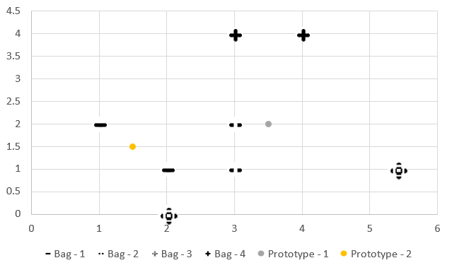
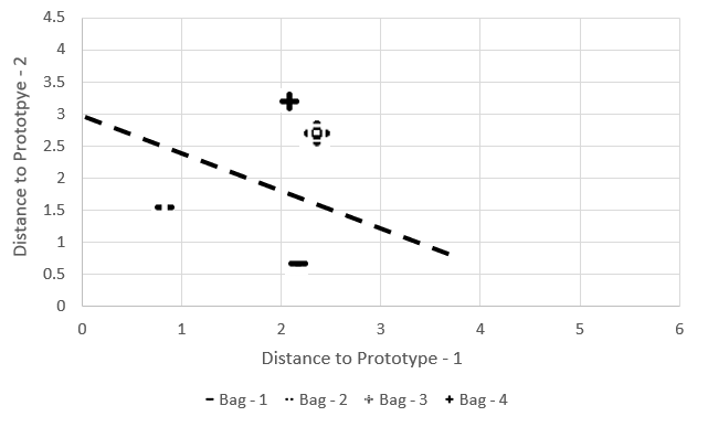
The model has two main objectives: First one is learning the feature vectors or prototypes that is maximally predictive of the bag class after finding an embedding in the distance space. A simple illustration of the idea is presented in Figure 1(a). Suppose there are two positive and two negative bags each of which have two instances in two-dimensional feature space shown in Figure 1(a). Our aim is to identify prototypes such that the bags are linearly separable when each bag is represented by its minimum distance to each prototype. Figure 1(b) represents the bags in the new feature space. In other words, proposed model is optimized over both the linear classifier parameters and the prototypes. An overview of architecture can be seen in Figure 2. Depending on the application, our proposal is flexible in generating average and maximum type of features which are famous in multiple instance learning domain (Cheplygina et al., 2015).

In terms of interpretability, Ilse et al. (2018) uses attention to give weights to instances in a bag and use these weights to do classification, hence in a sense one can interpret which instance contributes to the decision. One of the main contributions of our work is, we are able to extract meaningful prototypes in a dataset that represent classes. In other words, we are not only able to put meaningful weights on instances, but also we can extract the most predictive fragments in the dataset with respect to the task. After the training phase is complete, we can examine the prototypes to see what fragments are the most representative of the given class. Moreover, since we are not using a feedforward network to extract the features, but we are using the distances to each prototype as the features, we do not need a computationally expensive architecture. In other words, after calculating the distances to prototypes, we only use a simple linear layer to make a prediction.

(a) Bag 1 and Bag 2 are negative labeled bags. Bag 3 and Bag 4 have positive labels. All bags and prototypes have two features.

(b) Distances of bags to prototypes. A good prototype candidate separates negative and positive labeled bags.

Figure 1: Representation of Bags and Prototypes.

 

Figure 2: Overview of the architecture. Blue color shows the variables, which the model will be optimized over. $L$: Number of features in an instance, constant; $D$: Number of prototypes, hyperparameter; $K_{i}$: Number of instances bag i, varies between different bags

In our setting, for a given training task we choose a fixed number of prototypes, $D$, of a fixed size, $L$, to be learned, we initialize these prototypes randomly. We combine each instance of length $L$ in a given bag, which yields $K_{i}$(number of instances in bag i) vectors representing bag i. $K_{i}$ is not constant between different bags, since each bag potentially has different number of instances. At each training step, we calculate the distance from each instance to the prototypes to extract distance features. Given these features, the model learns a classifier to predict the bag class.

3.1.1 Distance Feature Extraction

Just as in instance-level approaches in MIL problems, our model also needs to pool information that is extracted from instances in a given bag with potentially variable number of instances. To be more specific, for a given bag after the distance from each instance to each prototype is calculated, the model needs to aggregate the information before being fed into a linear classifier. These pooling operations should be differentiable to be optimized with a gradient based approach. Most basic and widely used pooling operators having these characteristics are min, mean and max operators (Cheplygina et al., 2015). These are also intuitively informative in our case, since we have distance metrics as features, such that these should provide information about defining characteristics of an instance, assuming the existence of prototypes which are described above. After the distance extraction, we apply L2 regularization to all extracted distances, to minimize the distances. This is to ensure that the prototypes are as close to instances as possible and semantically meaningful. Our objective function for an example problem can be found in Appendix A Equation 1.

3.1.2 Feature Normalization

The distance features are prone to scale issues. This can cause problems with both gradient updates and the learning of linear classifier parameters. To overcome this, we adapt a similar approach to Ba et al. (2016), Ioffe and Szegedy (2015). In other words, for each bag, we normalize the aggregated distance vector. Note that the information related to "shape" of the distance features will be preserved under the normalization operation that is only recentering and rescaling, which is what we aim to achieve.
A detailed formulation of the described method can be found in Appendix A.

4 Experiments

Solution approach is tested on five MIL datasets from two categories, molecular activity prediction and image annotation. We repeat a stratified 10-fold cross-validation five times and report the average of the classification accuracy with standard error in Table 3. For all experiments, prototypes are generated randomly and logistic regression is used as default classifier. Important parameters are the number of prototypes to learn and learning rate for weights and prototypes. The model was implemented in PyTorch(Paszke et al., 2017) and we use the same parameters for each dataset. Namely, the number of epochs is set to 100 with a minibatch size of 1. Adam optimizer from (Kingma and Ba, 2015) was used. As mentioned above, we use different learning rates for the classifier and the prototypes. Regularization parameters and learning rates for each dataset can be found below.

	Musk1	Musk2	Fox	Tiger	Elephant
Learning Rate of Classifier	3e-5	4e-5	3e-5	1e-4	3e-5
Learning Rate of Prototypes	9e-5	8e-5	5e-5	3e-5	9e-5
$\lambda_{p}$ , Prototypes Regularization Parameter	4e-3	4e-3	4e-3	4e-3	4e-3
$\lambda_{d}$ , Distance Regularization Parameter	1e-2	1e-2	1e-2	1e-2	1e-2
$\lambda_{d}$ , Classifier Weight Regularization Parameter	3e-4	3e-4	3e-4	3e-4	3e-4
Number of prototypes	24	24	24	24	24

Table 2: Hyperparameters for different datasets.

4.1 Classification Accuracy

Solution approach in this study outperforms or at least does as good as all other well-known methods in terms of classification accuracy. Besides this approach has much less parameters compared to a neural network, namely only prototypes and few parameters for linear classifier.

	Musk1	Musk2	Fox	Tiger	Elephant
mi-SVM (Andrews et al., 2003)	0.874$\pm$N/A	0.836$\pm$N/A	0.582$\pm$N/A	0.784$\pm$N/A	0.822$\pm$N/A
MI-Kernel(Gartner et al., 2002)	0.880$\pm$0.031	0.893$\pm$0.015	0.603$\pm$0.028	0.842$\pm$0.010	0.843$\pm$0.016
EM-DD(Zhang and Goldman, 2002)	0.849$\pm$0.044	0.869$\pm$0.048	0.609$\pm$0.045	0.730$\pm$0.043	0.771$\pm$0.043
mi-Graph(Zhou et al., 2009)	0.889$\pm$0.033	0.903$\pm$0.039	0.620$\pm$0.044	0.860$\pm$0.037	0.869$\pm$0.035
miVLAD(Wei et al., 2017)	0.871$\pm$0.043	0.872$\pm$0.042	0.620$\pm$0.044	0.811$\pm$0.039	0.850$\pm$0.036
miFV(Wei et al., 2017)	0.909$\pm$0.040	0.884$\pm$0.042	0.621$\pm$0.049	0.813$\pm$0.037	0.852$\pm$0.036
MI-Net(Wang et al., 2018)	0.894$\pm$0.042	0.874$\pm$0.043	0.630$\pm$0.037	0.845$\pm$0.039	0.872$\pm$0.032
Attention(Ilse et al., 2018)	0.892$\pm$0.040	0.858$\pm$0.048	0.615$\pm$0.043	0.839$\pm$0.022	0.868$\pm$0.022
Gated-Attention(Ilse et al., 2018)	0.900$\pm$0.050	0.863$\pm$0.042	0.603$\pm$0.029	0.845$\pm$0.018	0.857$\pm$0.027
Prototype Learning	0.9083$\pm$0.107	0.942$\pm$0.070	0.691$\pm$0.100	0.916$\pm$0.0565	0.920$\pm$0.060

Table 3: Result comparison of different approaches.

4.2 Interpretability

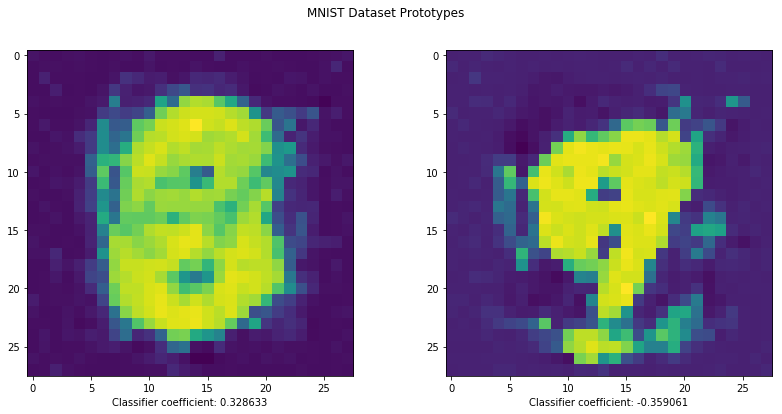
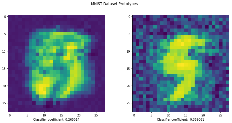
As indicated previously, interpretability of the solution is one of the main aspects of prototype learning. To demonstrate this interpretability, here we apply our approach to the MNIST MIL problem which was introduced in Ilse et al. (2018). In this case, each instance is an image and each bag consists of images. The task is finding whether a target number exists in images in a bag. To keep things simple, we chose the number of prototypes to be 2.

Examples of prototypes from 2 different runs can be seen in Figure 3(a). In this application, we only used $min$ as the aggregator for better interpretation. For instance, looking at Figure 3(a), we see that second prototype looks a lot like a 9, and the classifier found a negative coefficient for minimum distance to this prototype. This indicates, if the minimum distance to this prototype is larger the output probability will suffer. Moreover, since the first prototype has a positive coefficient, if the minimum distance of the bag to this prototype is larger, the output probability will be higher. Same analysis can be done for Figure 3(b).

(a) Prototype results when the method is applied to MNIST dataset with finding the 9 problem.

(b) Bags are labeled positive if number 5 is an instance in the bag.

Figure 3: MNIST Prototypes.

 

5 Conclusion

This work presents a prototype learning framework for MIL problems. This simple architecture can be applied to data from all kinds of domains and offers interpretability of the solutions. Although the method is applied to the classical MIL datasets, its modification to different problems is an interesting research direction. Our aim is to present the simplicity of the approach and hence sticked to the logistic regression classifiers and Euclidean distance. However, considering the flexibility of the architecture, one could incorporate more complex classifiers, different distance metrics and different aggregation procedures to obtain more powerful models.

Appendix A Method Formulation

Below we give a formulation for the discussed method. We will only demonstrate the formulation for $min$ features for simplicity, which could easily be generalized to any combination of $min$,$max$ and $mean$. Also below we use sigmoid for binary classification, but the same framework could easily be extended to multinomial case utilizing a softmax function.

$D\mathrel{\mathop{\mathchar 58\relax}}$ Number of prototypes
$K_{i}\mathrel{\mathop{\mathchar 58\relax}}$ Number of instances in bag $i$
$L\mathrel{\mathop{\mathchar 58\relax}}$ Number of features in any instance
$P\mathrel{\mathop{\mathchar 58\relax}}$ set of prototypes, $P_{d}$: $d^{th}$ prototype, a vector with length $L$
$X_{i}\mathrel{\mathop{\mathchar 58\relax}}$ set of instances in bag $i$, $X_{ik}$: $k_{th}$ instance in bag $i$
$y_{i}\mathrel{\mathop{\mathchar 58\relax}}$ Label, class of the bag $i$.
$Dist(v_{1},v_{2})\mathrel{\mathop{\mathchar 58\relax}}$ Distance between vectors $v_{1}$ and $v_{2}$
$\beta_{d}\mathrel{\mathop{\mathchar 58\relax}}$ Weight in linear classifier that corresponds to $d_{th}$ prototype
$\Phi_{id}$: $d^{th}$ element of the output vector for bag $i$. Corresponds to the minimum distance of bag $i$ to prototype $d$ after layer normalization.
$\sigma(Y)=\frac{1}{1+e^{-Y}}$ is the sigmoid function
$\mathcal{L}_{ce}(y_{i},\hat{y}_{i})\mathrel{\mathop{\mathchar 58\relax}}$ Cross-entropy loss where $y_{i}$ is the label and $\hat{y}_{i}$ is the prediction
$\lambda_{w}\mathrel{\mathop{\mathchar 58\relax}}$ Regularization parameter for linear classifier weights
$\lambda_{p}\mathrel{\mathop{\mathchar 58\relax}}$ Regularization parameter for prototypes
$\lambda_{d}\mathrel{\mathop{\mathchar 58\relax}}$ Regularization parameter for the extracted distances

$$\!\min_{P,\beta}\sum_{i=1}^{N}\mathcal{L}_{ce}(y_{i},\hat{y}_{i})+\lambda_{w}\mathinner{\!\left\lVert\beta\right\rVert}_{1}+\lambda_{p}\sum_{d=1}^{D}\mathinner{\!\left\lVert P_{d}\right\rVert}_{2}+\lambda_{d}\sum_{i=1}^{N}\sum_{d=1}^{D}\Phi_{id}$$ (1)

$$\Phi_{id}=\min_{X_{ik}\in X_{i}}Dist(X_{ik},P_{d})$$ (2)

$$\hat{y}_{i}=\sigma(\beta_{0}+\sum_{d=1}^{D}\beta_{d}\Phi_{id})$$ (3)

The objective function given in Equation 1 is optimized over the prototypes, $P$, and the linear classifier weights, $\beta$. Different lea rning rates are used for prototypes and the classifier parameters, namely $\alpha_{w}$ for weights and $\alpha_{p}$ for prototypes. The model is trained for 100 epochs, minibatch size 1 is used with Adam optimizer [Kingma and Ba, 2015] .

We also perform layer normalization. Namely, each row in the transformed distance space is scaled to zero mean and unit variance as illustrated in Equations 4a, 4b. Layer normalization is important because it stabilizes the issues that could occur during optimization due to the scale of distance features and it reduces the sensibility of linear classifier to the scale of distances but it keeps the relative distance information. As a side benefit, we observe that as argued in [Ba et al., 2016], it speeds up the convergence.

$$\mu_{i}=\frac{1}{D}\sum_{d=1}^{D}\Phi_{id},\sigma_{i}=\sqrt{\frac{1}{D}(\Phi_{i}-\mu_{i})^{2}}$$ (4a)

$$\Phi_{i}=\frac{\Phi_{i}-\mu_{i}}{\sigma_{i}}$$ (4b)

The parameters of our experiments are as the following: $D=24$, $\lambda_{p}=0.05$, $\lambda_{w}=0.05$, $Dist$ calculates Euclidean distance, $\alpha_{p}=0.0001$, $\alpha_{w}=0.00005$. In practice, any differentiable distance metric could be used in this framework with gradient based optimization methods.

References

- Dietterich et al. [2001] Thomas Dietterich, Richard H. Lathrop, and Tomás Lozano-Pérez. Solving the multiple instance problem with axis-parallel rectangles. Artificial Intelligence, 89:31–71, 03 2001.
- Weidmann et al. [2003] Nils Weidmann, Eibe Frank, and Bernhard Pfahringer. A two-level learning method for generalized multi-instance problems. Machine Learning: ECML, pages 468–479, 2003.
- Li et al. [2013] Yan Li, David M.J. Tax, Robert P.W. Duin, and Marco Loog. Multiple-instance learning as a classifier combining problem. Pattern Recognition, 46(3):865 – 874, 2013.
- Wang and Zucker [2000] Jun Wang and Jean-daniel Zucker. Solving the multiple-instance problem: A lazy learning approach. Proc. 17th International Con. on Machine Learning, pages 1119–1126, 01 2000.
- Xu and Frank [2004] X. Xu and E. Frank. Logistic regression and boosting for labeled bags of instances. Proceedings of the Eighth Pacific-Asia Conference on Knowledge Discovery and Data Mining, pages 272–281, 2004.
- Xu [2003] X. Xu. Statistical learning in multiple instance problems (m.sc. thesis), university of waikato. University of Waikato, 2003.
- Raykar et al. [2008] V.C. Raykar, B. Krishnapuram, J. Bi, M. Dundar, and R.B. Rao. Bayesian multiple instance learning: Automatic feature selection and inductive transfer. Proceedings of the 25th International Conference on Machine Learning, ACM, New York, NY, pages 808–815, 2008.
- Amores [2013] J. Amores. Multiple instance classification: Review, taxonomy and comparative study. Artificial Intelligence 201, pages 81–105, 2013.
- Zhou et al. [2005] Z. Zhou, K. Jiang, and M. Li. Multi-instance learning based web mining. Applied Intelligence, 22(2):135–147, 2005.
- Cheplygina et al. [2013] Veronika Cheplygina, David Tax, and Marco Loog. Combining instance information to classify bags. Multiple Classifier Systems, submitted, 05 2013.
- Cheplygina et al. [2016] V. Cheplygina, D. M. J. Tax, and M. Loog. Dissimilarity-based ensembles for multiple instance learning. IEEE Transactions on Neural Networks and Learning Systems, 27(6):1379–1391, June 2016.
- Gehler and Chapelle [2007] Peter Gehler and Olivier Chapelle. Deterministic annealing for multiple-instance learning. 2007.
- Ilse et al. [2018] Maximilian Ilse, Jakub Tomczak, and Max Welling. Attention-based deep multiple instance learning. 80:2127–2136, 10–15 Jul 2018. URL http://proceedings.mlr.press/v80/ilse18a.html.
- Wang et al. [2018] Xinggang Wang, Yongluan Yan, Peng Tang, Xiang Bai, and Wenyu Liu. Revisiting multiple instance neural networks. Pattern Recogn., 74(C):15–24, February 2018. ISSN 0031-3203. doi: 10.1016/j.patcog.2017.08.026. URL https://doi.org/10.1016/j.patcog.2017.08.026.
- Wu et al. [2015] J. Wu, Yinan Yu, Chang Huang, and Kai Yu. Deep multiple instance learning for image classification and auto-annotation. In 2015 IEEE Conference on Computer Vision and Pattern Recognition (CVPR), pages 3460–3469, June 2015. doi: 10.1109/CVPR.2015.7298968.
- Tang et al. [2018] Peng Tang, Xinggang Wang, Song Bai, Wei Shen, Xiang Bai, Wenyu Liu, and Alan L. Yuille. PCL: proposal cluster learning for weakly supervised object detection. CoRR, abs/1807.03342, 2018. URL http://arxiv.org/abs/1807.03342.
- Wan et al. [2019] Fang Wan, Chang Liu, Wei Ke, Xiangyang Ji, Jianbin Jiao, and Qixiang Ye. C-MIL: continuation multiple instance learning for weakly supervised object detection. CoRR, abs/1904.05647, 2019. URL http://arxiv.org/abs/1904.05647.
- Dennis et al. [2018] Don Kurian Dennis, Chirag Pabbaraju, Harsha Vardhan Simhadri, and Prateek Jain. Multiple instance learning for efficient sequential data classification on resource-constrained devices. In Proceedings of the 32Nd International Conference on Neural Information Processing Systems, NIPS’18, pages 10976–10987, USA, 2018. Curran Associates Inc. URL http://dl.acm.org/citation.cfm?id=3327546.3327753.
- Angelidis and Lapata [2017] Stefanos Angelidis and Mirella Lapata. Multiple instance learning networks for fine-grained sentiment analysis. CoRR, abs/1711.09645, 2017. URL http://arxiv.org/abs/1711.09645.
- McFee et al. [2018] Brian McFee, Justin Salamon, and Juan Pablo Bello. Adaptive pooling operators for weakly labeled sound event detection. CoRR, abs/1804.10070, 2018. URL http://arxiv.org/abs/1804.10070.
- Cheplygina et al. [2015] Veronika Cheplygina, David M.J. Tax, and Marco Loog. Multiple instance learning with bag dissimilarities. Pattern Recognition, 48(1):264 – 275, 2015.
- Ba et al. [2016] Lei Jimmy Ba, Jamie Ryan Kiros, and Geoffrey E. Hinton. Layer normalization. CoRR, abs/1607.06450, 2016. URL http://arxiv.org/abs/1607.06450.
- Ioffe and Szegedy [2015] Sergey Ioffe and Christian Szegedy. Batch normalization: Accelerating deep network training by reducing internal covariate shift. In Proceedings of the 32Nd International Conference on International Conference on Machine Learning - Volume 37, ICML’15, pages 448–456. JMLR.org, 2015. URL http://dl.acm.org/citation.cfm?id=3045118.3045167.
- Paszke et al. [2017] Adam Paszke, Sam Gross, Soumith Chintala, Gregory Chanan, Edward Yang, Zachary DeVito, Zeming Lin, Alban Desmaison, Luca Antiga, and Adam Lerer. Automatic differentiation in pytorch. 2017.
- Kingma and Ba [2015] Diederik P. Kingma and Jimmy Ba. Adam: A method for stochastic optimization. In 3rd International Conference on Learning Representations, ICLR 2015, San Diego, CA, USA, May 7-9, 2015, Conference Track Proceedings, 2015. URL http://arxiv.org/abs/1412.6980.
- Andrews et al. [2003] S. Andrews, T. Hofmann, and I. Tsochantaridis. Support vector machines for multiple-instance learning. Advances in Neural Information Processing Systems 15, pages 561–568, 2003.
- Gartner et al. [2002] T Gartner, PA Flach, A Kowalczyk, and AJ Smola. Multi-Instance Kernels, pages 179 – 186. Morgan Kaufmann, 7 2002.
- Zhang and Goldman [2002] Q. Zhang and S. Goldman. Em-dd: An improved multiple-instance learning technique. Advances in Neural Information Processing Systems, 14, 2002.
- Zhou et al. [2009] Z.H. Zhou, Y.Y. Sun, and Y.F. Li. Multi-instance learning by treating instances as non-iid samples. Proceedings of International Conference on Machine Learning (ICML), pages 1249–1256, 01 2009.
- Wei et al. [2017] Xiu-Shen Wei, Jianxin Wu, and Zhi-Hua Zhou. Scalable algorithms for multi-instance learning. IEEE transactions on neural networks and learning systems, 28(4):975–987, 2017.