Model Order Reduction for
Efficient Descriptor-Based Shape Analysis

Abstract

In order to investigate correspondences between 3D shapes, many methods rely on a feature descriptor which is invariant under almost isometric transformations. An interesting class of models for such descriptors relies on partial differential equations (PDEs) based on the Laplace-Beltrami operator for constructing intrinsic shape signatures. In order to conduct the construction, not only a variety of PDEs but also several ways to solve them have been considered in previous works. In particular, spectral methods have been used derived from the series expansion of analytic solutions of the PDEs, and alternatively numerical integration schemes have been proposed.

In this paper we show how to define a computational framework by model order reduction (MOR) that yields efficient PDE integration and much more accurate shape signatures as in previous works. Within the construction of our framework we introduce some technical novelties that contribute to these advances, and in doing this we present some improvements for virtually all considered methods. As part of the main contributions, we show for the first time an extensive and detailed comparison between the spectral and integration techniques, which is possible by the advances documented in this paper. We also propose here to employ soft correspondences in the context of the MOR methods which turns out to be highly beneficial with this approach.

1 Introduction

The investigation of correspondences between 3D shapes is a fundamental problem in computer vision, graphics and pattern recognition. It has a wide variety of potential applications, including e.g. shape comparison or texture transfer, see e.g. vanKaick-etal-2011 for some discussion. The basic task of finding shape correspondences is to identify a relation between elements of two or more shapes, and a challenging setting for this is concerned with non-rigid shapes that are assumed to be just almost isometric, compare for instance TOSCA .

One of the possible strategies to find pointwise correspondences is to construct a feature descriptor, or shape signature, which characterises geometry around the points that define the surface of a given shape. An interesting type of such approaches relies on the Laplace-Beltrami operator which enables to describe intrinsic geometric properties of a shapes’ surface Levy-2006 ; Reuter-etal-2009 ; R . To this end, several partial differential equations (PDEs) have been proposed for the construction of shape signatures that rely on the Laplace-Beltrami operator as a crucial component. The heat kernel signature (HKS) introduced in SOG is based on the heat equation, the wave kernel signature (WKS) ASC is constructed using the Schrödinger equation, and recently the classic wave equation DBH-2017 has been applied.

The mentioned kernel-based signatures (HKS and WKS) are computed using the kernels of analytic solutions of the underlying PDEs, resulting in infinite series expansions that define the complete solutions in time at a given surface point. Let us note that it is not immediately evident when to truncate the series for practical purposes, yet some strategies have been given in the literature TOSCA ; see also DBH-2018 for a recent, related investigation. As an alternative approach to the kernel-based methods, the full numerical integration of the PDEs has been considered DBH-2016 , and the abovementioned shape signature defined via the classic wave equation DBH-2017 has been realised in this setting. Comparing these two approaches, the numerical integration as reported in DBH-2017 ; DBH-2016 may yield a more accurate correspondence, while the computation of the numerical signatures has been much more time-consuming than the kernel-based signatures. In order to improve the performance of the integration approach, a model order reduction (MOR) technique has been proposed in BDB-2018 , showing some promising first results.

Our Contribution

The goal of this paper is to document several substantial advances of the integration based approach. Based on these improvements, we also give here a much more detailed comparison to kernel-based methods than it was possible before. More concretely, let us mention the following main points, clarifying at the same time relation to previous literature:

(i) Employing the MOR technique introduced in BDB-2018 for the shape matching purpose, we show that it pays off to extend the considered time scale in the numerical MOR signatures. The large time scales we employ here for the first time with the MOR signature yields a notable improvement in quality of results.

(ii) We introduce a numerical similarity transform within both the MOR and kernel-based signatures which yields a much more stable computation as well as in most cases results of much higher accuracy for all considered techniques.

(iii) Since the MOR method is highly efficient, it is now possible to evaluate much larger datasets conveniently. We present here for the first time a thorough evaluation and comparison of the mentioned methods at hand of the complete TOSCA dataset.

(iv) We investigate here for the first time soft correspondences for use with the MOR signatures. The soft correspondences are derived from soft maps Eisenberger2018 ; SNBBG-2012 . At hand of dedicated evaluations we show that the MOR technique works very favourably with this technique to establish correspondences.

(v) Because of the significantly better stability that is achieved via the introduced numerical similarity transform, it turns out we gain much more efficient computational approaches for all the methods in virtually all of the considered settings, as the problem dimensions that are of interest can be reduced (except for the kernel-based methods when evaluating the geodesic error measure in some experiments where we do not observe much improvement).

Let us note that in addition, in all of these points we introduce novel aspects and techniques compared to BDB-2018 . Especially, the extended experimental evaluations presented here allow to highlight some relevant properties of the MOR signature that have not been discussed earlier in BDB-2018 . As indicated in point (v) above, our results also shed light on the number of eigenvalues that should be employed within all of the mentioned techniques when using the numerical similarity transform as indicated above. This is an important practical issue for the discussed methods for pointwise shape correspondence.

Paper Organisation

After a broader exposition on related work on shape descriptors, we briefly recall the general framework we rely on along with the arising PDEs and the numerical discretisations employed in space and time. As our work relies very much on related numerical techniques, we give a comprehensive discussion of numerical solvers with an emphasis on solvers for the occurring specific linear systems of equations. In Section 6 we proceed with a detailed exposition of MOR methods and some related issues in our setting. Our first experimental evaluation presented in Section 7 focuses on the evaluation of solvers in the context of MOR techniques and time integration. This is followed by a discussion of the numerical similarity transform and time rescaling we propose here for optimisation. Beginning with Section 9 we include the kernel-based methods in our discussion. In Section 10 we give a detailed exposition of the comparison of the presented approaches, focusing thereby on the most promising MOR methods identified in the previous sections, and including the soft correspondence techniques. The paper is finished by a summary with a conclusion.

2 More on Related Work

A large variety of feature descriptors for 3D objects has been proposed in the fields of computer vision, pattern recognition and computer graphics within the last decades. The classic feature descriptors handle rigid transformations while more recent approaches on which we focus are invariant under isometric transformations. Furthermore, one may identify in a broad sense four classes as follows.

Distance-Based Methods

In OFCD a descriptor is proposed that uses the distribution of the Euclidean distances between pairs of randomly selected points on the surface of a 3D model. Other approaches use intrinsic properties of the shape by collecting information from intrinsic distances KS ; SSKG . Later, a pose-invariant shape descriptor is introduced in GSC as a 2D histogram estimated from the measure of the diameter of the 3D shape in the neighbourhood of each point on a surface and the average intrinsic distance from one point to all other points on the shape. The authors in IAPKC introduced a feature descriptor based on the distribution of the lengths of the longest geodesics on the shape. Finally, COO introduced a multiscale signature based on the topological structure of the distribution of geodesic distances centred at a given point.

Local Descriptors

The idea of local descriptors is to characterise each point on a shape by using local geometric properties. Important classic examples of local point-based signatures are the well-known spin images JH and shape context BMP . Later, a multi-scale version of the local neighbourhood of the given point was used in YLHP to construct a feature descriptor. The authors in PWHY employed this approach for the computation of integral invariant features MHYS . In ZBH , the well-known SIFT descriptor Lowe-2004 which is based on locally computed features is extended to 3D objects. A similar feature descriptor, called SHOT, which describes the local shape structure by a collection of the distribution of normal directions, was introduced in TSS . Finally, among the newer methods, there is the Anisotropic Windowed Fourier Transform (AWFT) descriptor MRCB . Starting from a collection of functions, the descriptors are obtained as a weighted linear combination of the coefficients of the AWFT.

Time-Evolution Methods

Another trend in shape analysis consists of exploiting intrinsic time evolution processes carried by partial differential equations on geometric shapes. In this context diffusion processes are well established, allowing a meaningful interpretation relating the propagation of information and intrinsic distances. For example, the propagation of heat on a shape can be interpreted as a random walk among surface points CL ; BB-2011 . In the spirit of this framework, SOG introduced the HKS. The HKS describes the amount of heat remaining at a certain point after a certain amount of time. The geometric interpretation of this approach is that one can determine a connection between the heat kernel and intrinsic distances via Varadhan’s formula Varadhan1967 . Later, a scale invariant extension of the HKS was developed BK-2010 . In ASC another feature descriptor namely the WKS inspired by equations of theoretical physics is proposed. Based on the Schrödinger equation, the WKS represents the average probability of measuring a quantum mechanical particle at a specific location. At the same time, BB-2011 proposed a scheme that is able to generalise the diffusion-based approaches.

All of these methods are based on the spectral decomposition of the Laplace-Beltrami operator on manifold shapes. To this end, the feature descriptors can be represented by a truncated series using the eigenvalues and eigenfunctions of the Laplace-Beltrami operator. In MORCC the authors developed a feature descriptor using a specific discrete diffusion process without truncating an eigendecomposition. As indicated in the introduction, some works have been proposed to avoid the need for the latter by introducing an alternative method based on the full discretisation of the underlying PDEs DBH-2017 ; DBH-2016 at the expense of additional computation time, when considering all points on the shape.

Learning-Based Methods

Feature descriptors based on intrinsic time-evolution methods are invariant to isometric transformations. However, in applications elastic deformations may appear yielding some distortions in intrinsic distances. In order to address this problem, a class of methods has been introduced by using the learning-by-example approach. In LB-2014 , the so-called optimal point descriptor is proposed. The technique proposed in KIDS relies on random forests. In COC-2014 , a learning procedure has been introduced within the functional map framework, and in LBBC the authors proposed a learning strategy in the context oft the bag-of-word framework. Finally, BMMBCV introduced a matching method that extends convolutional neural networks to the spectral domain.

Some Remarks on Other Related Approaches

Let us note that point or shape signatures can also be used within other important methods for shape correspondence that are extensions of classical point-to-point mappings. As examples let us mention the works based on functional maps OBSBG where correspondences are modelled as linear operators between spaces of functions on manifolds. In the technical context of functional maps let us also mention the use of product manifolds VLRBC . The functional map framework has been adopted and extended in several follow-up works ERGB ; MRSWO ; RCBTC ; RLBBS with extensions to learning based techniques HLRBK ; LRRBB relating to the corresponding category as above.

3 About the Shape Correspondence Framework

In this section we introduce the basic facts that are necessary to define the shape correspondence framework. Concerning the general shape analysis set-up, we largely follow concepts as discussed for instance in TOSCA . For notions from differential geometry as employed here we refer the reader to DC .

3.1 Almost Isometric Shapes

A three-dimensional geometric shape can be described by its bounding surface. Thus, our shape model consists of compact two-dimensional Riemannian manifolds $\mathcal{M}\subset\mathbb{R}^{3}$, equipped with the metric tensor $g\in\mathbb{R}^{2\times 2}$ that describes locally the geometry.

Two shapes $\mathcal{M}$ and $\widetilde{\mathcal{M}}$ may be considered as isometric if there is a smooth homeomorphism $T\mathrel{\mathop{\mathchar 58\relax}}\mathcal{M}\rightarrow\widetilde{\mathcal{M}}$ between the corresponding object surfaces that preserves the intrinsic distances between surface points:

$$d_{\mathcal{M}}(x_{1},x_{2})=d_{\mathcal{\widetilde{M}}}(T(x_{1}),T(x_{2})),\quad\forall x_{1},x_{2}\in\mathcal{M}$$ (1)

The intrinsic distance between two surface points $x_{k}$, $k=1,2$ may be interpreted as the shortest path along the surface $\mathcal{M}$ connecting $x_{1}$ and $x_{2}$.

In many applications, the notion of isometric shapes may be too restrictive. For instance, small noise in a dataset could be considered as an elastic deformation yielding some distortions in intrinsic distances. To take into account this issue, we call two shapes $\mathcal{M}$ and $\widetilde{\mathcal{M}}$ almost isometric, if there exists a transformation $S\mathrel{\mathop{\mathchar 58\relax}}\mathcal{M}\rightarrow\widetilde{\mathcal{M}}$ with

$$d_{\mathcal{M}}(x_{1},x_{2})\approx d_{\mathcal{\widetilde{M}}}(S(x_{1}),S(x_{2})),\quad\forall x_{1},x_{2}\in\mathcal{M}$$ (2)

3.2 PDE-based Models for Shape Description

A classic but still modern descriptor class that can handle almost isometric transformations relies on physical models that are conveniently described by PDEs. In the following, we introduce the two fundamental PDEs that we employ to this end.

The geometric heat equation that yields a useful shape descriptor SOG involves the Laplace-Beltrami operator. This is the geometric version of the Laplace operator that takes into account the curvature of a smooth manifold in 3D. Given a parametrisation of such a two-dimensional manifold, the Laplace-Beltrami operator applied to a scalar function $u\mathrel{\mathop{\mathchar 58\relax}}\mathcal{M}\rightarrow\mathbb{R}$ can be expressed in local coordinates as

$$\Delta_{\mathcal{M}}\,u={\frac{1}{{\sqrt{|g|}}}}\sum_{i,j=1}^{2}\partial_{i}\left({\sqrt{|g|}}g^{{ij}}\partial_{j}u\right)$$ (3)

where $g^{ij}$ are the entries of the inverse of the metric tensor and $|g|$ is its determinant. Using this the geometric heat equation reads as

$$\partial_{t}u(x,t)=\Delta_{\mathcal{M}}\,u(x,t),\qquad x\in\mathcal{M},\;t\in I$$ (4)

and describes how heat would diffuse along a surface $\mathcal{M}$.

The geometric wave equation is the second PDE that is going to be discussed in this work. It has been introduced in DBH-2017 as a useful model for computing pointwise a shape descriptor. Assuming the speed of wave propagation is identical to one in all directions on the manifold, the corresponding PDE is

$$\partial_{tt}u(x,t)=\Delta_{\mathcal{M}}\,u(x,t),\qquad x\in\mathcal{M},\;t\in I$$ (5)

Both of the described PDEs require an initial condition in order to be meaningful. In the context of shape correspondence construction, we employ a Dirac delta function $u(x,0)=u_{0}(x)=u_{x_{i}}$ centred around a point of interest $x_{i}\in\mathcal{M}$. The PDE (5) is of second order in time, so that it needs to be supplemented not only by a spatial function as an initial state, but also an account of the initial velocity of that initial state is needed. As it is a canonical choice, we consider the zero initial velocity condition $\partial_{t}u(x,0)=0$.

Let us note that many shapes appear as a closed manifold with $\partial\mathcal{M}=\emptyset$, where it is not necessary to define additional boundary conditions. For the case $\mathcal{M}$ has boundaries, we may require $u$ to satisfy homogeneous Neumann boundary conditions.

3.3 Feature Descriptor and Shape Correspondence

We now make precise how geometric feature descriptors are obtained by employing the introduced PDEs, and how we construct shape correspondence on that basis.

Feature Descriptor

For many shape analysis tasks, it is useful to consider a pointwise feature descriptor as a shape representation. The purpose of the feature descriptor is to give an account of the geometry of the surface at a certain local region centred about a considered point. To this end, we restrict the spatial component of solutions $u(x,t)$ of the introduced PDEs to

$$f_{x_{i}}(t)\mathrel{\mathop{\mathchar 58\relax}}=u(x,t)_{\mid_{x=x_{i}}}\quad\mbox{with}\quad u(x,0)_{\mid_{x=x_{i}}}=u_{x_{i}}$$ (6)

and call the $f_{x_{i}}$ the feature descriptors at the location $x_{i}\in\mathcal{M}$.

Let us comment that there exists a physical interpretation related to the feature descriptors we employ. The heat based feature descriptor $f_{x_{i}}$ describes the rate of heat transferred away from the considered point $x_{i}$. The spreading of heat takes into account the geometry of the surface by using the Laplace-Beltrami operator. In turn, the wave based feature descriptor describes the motion amplitudes of an emitted wave front observed at the considered point $x_{i}$ during time evolution. Therefore, the latter feature descriptor catches the typical wave interaction observable in the solution of the wave equation as can e.g. be seen in the well-known formula of d’Alembert in the 1D case. Analogously to the situation for the heat-based descriptor, the observable motion of the waves is influenced by the intrinsic geometry of the surface. As time evolves, the waves spread over the surface so that their amplitude observed via $f_{x_{i}}(t)$ have the tendency to decrease.

Let us note that the feature descriptors discussed in this work cannot distinguish between intrinsic symmetry groups as they rely on intrinsic shape properties.

Shape Correspondence

To compare the feature descriptors for different locations $x_{i}\in\mathcal{M}$ and $\widetilde{x}_{j}\in\widetilde{\mathcal{M}}$ on respective shapes $\mathcal{M}$ and $\widetilde{\mathcal{M}}$ , we employ a distance $d_{f}(x_{i},\widetilde{x}_{j})$ using the $L_{1}$ norm as

$$d_{f}(x_{i},\widetilde{x}_{j})=\int\limits_{I}|f_{x_{i}}-f_{\widetilde{x}_{j}}|\,\mathrm{d}t$$ (7)

It is clear that the tuple of locations $(x_{i},\widetilde{x}_{j})\in\mathcal{M}\times\widetilde{\mathcal{M}}$ with the smallest feature distance should belong together. This consideration naturally leads to a minimisation problem for all locations:

$$(x_{i},\widetilde{x}_{j})=\operatorname*{arg\,min}\limits_{\widetilde{x}_{k}\in\mathcal{\widetilde{M}}}\,d_{f}(x_{i},\widetilde{x}_{k})$$ (8)

By using $\widetilde{x}_{j}=S(x_{i})=x_{i}$, the map $S$ can pointwise be restored for all $x_{i}$. Let us comment that without further alignment it cannot be expected that the restored map $S$ is injective or surjective, since the minimisation condition is not unique.

4 Basic Discretisation of Continuous-scale Models

In this section we recall the basics of the discretisation of the PDEs we employ. In order to prepare for later developments that are at the heart of the contributions of this paper, let us note that we really give just the description of the fundamentals. The concrete schemes used for computations are relying on the technical building blocks we introduce here.

4.1 Discretising in Space and Time

The discrete surface representation for computations is given by a triangular mesh which we denote as $\mathcal{M}_{d}=(P,T)$, cf. Figure 2. The underlying point cloud $P\mathrel{\mathop{\mathchar 58\relax}}=\{x_{1},\ldots,x_{N}\}$ contains a finite number of vertices in terms of coordinate points. The mesh is constructed by connecting the vertices $x_{i}$ so that one obtains triangular cells. The individual triangles $T$ contain the neighbourhood relations between corresponding vertices. As visualised in Figure 2, we let $\Omega_{i}$ be the barycentric cell volume surrounding the $i$-th vertex.

Turning from space to time discretisation, we define time intervals $I_{k}=[t_{k-1},t_{k}]$ and set $t_{0}=0$ for subdividing the complete integration time $[0,t_{M}]$.

4.2 Finite Volumes: Semi-Discrete Form

Letting for the moment $\partial_{*}$ be either $\partial_{t}$ or $\partial_{tt}$, we consider the PDEs (4) and (5) over a so-called control volume $\Omega_{i}$ and a time interval $I_{k}$. Integration in space and time yields

$$\int\limits_{I_{k}}\int\limits_{\Omega_{i}}\partial_{*}u(x,t)\,\mathrm{d}x\,\mathrm{d}t=\int\limits_{I_{k}}\int\limits_{\Omega_{i}}\Delta_{\mathcal{M}}\,u(x,t)\,\mathrm{d}x\,\mathrm{d}t$$ (9)

In a finite volume method the quantities that are considered in computations are cell averages, i.e. for the $i$-th control volume, or cell, we define

$$u_{i}(t)=u(\bar{x}_{i},t)=\dfrac{1}{|\Omega_{i}|}\int\limits_{\Omega_{i}}u(x,t)\,\mathrm{d}x$$ (10)

where $|\Omega_{i}|$ denotes the area of the $i$-th control volume. Therefore, we define the averaged Laplacian as

$$Lu_{i}(t)=\frac{1}{|\Omega_{i}|}\int\limits_{\Omega_{i}}\Delta_{\mathcal{M}}\,u(x,t)\,\mathrm{d}x$$ (11)

As for the meaning of the latter integral on the right hand side, one has to apply the divergence theorem to substitute the volume integral into a line integral over the boundary of the cell volume.

For discretisation of the arising integral quantities, we employ here the widespread cotangent weight scheme as introduced in MDSB , which we briefly recall now.

Figure 1: Continuous and discrete shape representation (Figure adopted from BDB-2018 ). The discrete shape is given by non-uniform linear triangles. Volume cells as shown here in green are constructed by using the barycentric area around a vertex.

Figure 2: The cotangent weight scheme as discretisation of the Laplace-Beltrami operator (Figure adopted from BDB-2018 ). Left: interior edge. Right: boundary edge.

The arising discrete Laplace-Beltrami operator $L\in\mathbb{R}^{N\times N}$ is composed of the sparse matrix representation that can be written as $L=D^{-1}W$. The appearing symmetric weight matrix $W$ contains the entries

$$W_{ij}={\begin{cases}-\sum\limits_{j\in N_{i}}w_{ij},&{\mbox{if }}i=j\\ \phantom{-}w_{ij},&{\mbox{if }}i\neq j\text{ and }j\in N_{i}\\ \phantom{-}0,&{\mbox{else}}\end{cases}}$$ (12)

where $N_{i}$ denotes the set of points adjacent to the vertex $x_{i}$. The weights $w_{ij}$ of the edge $(i,j)$ between corresponding vertices distinguish between interior $E_{i}$ and boundary edges $E_{b}$ as shown in Figure 2, and are given as

$$w_{ij}={\begin{cases}\displaystyle{\frac{\cot\alpha_{ij}+\cot\beta_{ij}}{2}},&{\mbox{if }}(i,j)\in E_{i}\\ \displaystyle{\frac{\cot\alpha_{ij}}{2}},&{\mbox{if }}(i,j)\in E_{b}\end{cases}}$$ (13)

Furthermore, we let $\alpha_{ij}$ and $\beta_{ij}$ denote the two angles opposite to the edge $(i,j)$. The matrix

$$D=\text{diag}\left(|\Omega_{1}|,\ldots,|\Omega_{i}|,\ldots,|\Omega_{N}|\right)$$ (14)

contains the local volume cell areas.

Let us stress that $L$ is finally not symmetric. This fact has a significant influence on the computational setting that will arise and which we discuss in detail later.

Lastly, we now put together and summarise the components of the discretisation as we developed it until now. In this way we will end up with a semi-discrete form of the scheme.

Let a function defined on all cells be represented by now as an $N$-dimensional vector

$$\mathbf{u}(t)=(u_{1}(t),\ldots,u_{N}(t))^{\top}$$ (15)

Rewriting (9) using volume cell averages we obtain a system of ordinary differential equations (ODEs), one for each control volume:

$$\overset{*}{\mathbf{u}}(t)\,=\,L\mathbf{u}(t)\qquad\textrm{where}\qquad\overset{*}{\mathbf{u}}(t)=\displaystyle{\frac{d^{*}\mathbf{u}(t)}{d^{*}t}}$$ (16)

In order to clearly comment on the notation, the use of the star derivative $\overset{*}{\mathbf{u}}$ indicates the time derivatives of first and second order, respectively, as introduced in (9).

Standard methods for the numerical solution of (16) deal in general directly with first-order ODE systems. For the geometric heat equation the system (16) reads as

$$\mathbf{\dot{u}}(t)\,=\,L\mathbf{u}(t)$$ (17)

In contrast, the geometric wave equation is of second order, and a transformation into a first-order system

$$\mathbf{\dot{q}}(t)=K\mathbf{q}$$ (18)

with

$$K=\begin{pmatrix}0&I\\ L&0\end{pmatrix}\in\mathbb{R}^{2N\times 2N}$$ (19)

where $I\in\mathbb{R}^{N\times N}$ is the identity matrix and

$$\mathbf{q}(t)=(\mathbf{q_{1}}(t),\mathbf{q_{2}}(t))^{\top}=(\mathbf{u}(t),\mathbf{\dot{u}}(t))^{\top}$$ (20)

is necessary.

Let us now turn to the discrete initial conditions of the described time evolutions. The initial velocity function $\mathbf{\dot{u}}(0)$ for use with the geometric wave equation is identical to zero. Thus we have only to describe here the discrete setting for the initial spatial density $\mathbf{u}(0)$ which is used for both the geometric heat and wave equation. To this end, we have to construct a discretised version of the Dirac delta function we formally employed in the continuous-scale model. Using the cell average

$$\int\limits_{\Omega_{i}}u(x,0)\,\mathrm{d}x=1$$ (21)

where $u(x,0)$ may be interpreted now as a box function with unit area, being expressed as

$$u(x,0)={\begin{cases}\frac{1}{\mathinner{\!\left\lvert\Omega_{i}\right\rvert}},&{\mbox{if }}x\in\Omega_{i}\\ 0,&{\mbox{else }}\end{cases}}$$ (22)

the initial condition at the location $x_{i}$ can be formulated as

$$\mathbf{u_{x_{i}}}=\mathbf{u}(x_{i},0)=(0,\dots,0,|\Omega_{i}|^{-1},0,\dots,0)^{\top}$$ (23)

that implicitly bears a dependence on the index $i$. If we want to stress this dependence, we write the latter as $\mathbf{u_{i,0}}$.

4.3 Discrete Time Integration

Solving the arising ODE systems (17) and (18), respectively, involves the application of numerical integration and can be done by using time stepping methods. Widely used time integration schemes are the explicit Euler method, the implicit Euler method and the trapezoidal rule known as Crank-Nicolson method.

Explicit schemes require low computational effort when resolving one time step, but they are just conditionally stable and may suffer from small time step restrictions, see e.g. Smith1985 . As we have shown in our conference paper BDB-2018 , even recent explicit generalisations like the fast semi-iterative (FSI) method from HOWR2016 perform in an inefficient way when applied for shape matching. The main reason is that in typical discrete meshes representing shapes, one has to face in general a large variety of mesh widths, and especially also very small mesh widths arise. Since the spatial mesh width and the allowed time step size of explicit methods are coupled, exactly this issue makes the explicit methods not attractive in our setting. Let us note that this is the difference to the original setting in image processing from HOWR2016 , where the typical image processing setting with a uniform mesh width of one is employed.

In contrast, implicit methods like the implicit Euler method and the Crank-Nicolson method are by theory unconditionally stable but they require to solve a system of linear equations. Often the Crank-Nicolson method is used in applications due to its second-order convergence in time. However, the latter method is not $L_{0}$-stable which may result in undesirable oscillations in the numerical solution for problems with discontinuous initial conditions, compare Smith1985 . This happens to be the setting of interest in our approach. In such a case, usually $L_{0}$-stable schemes are preferred such that the implicit Euler method, as DBH-2017 ; DBH-2016 has shown, represents a reasonable choice for our purpose.

In the total, and as a consequence of the first investigations in BDB-2018 , we consider here only the implicit Euler method for the numerical solution of the underlying geometric PDEs.

Implicit Euler Method for the Geometric Heat Equation

First the application of the fundamental lemma of calculus for the left-hand-side of (17) gives us

$$\int\limits_{I_{k}}\mathbf{\dot{u}}(t)\,\mathrm{d}t=\int\limits_{t_{k-1}}^{t_{k}}\mathbf{\dot{u}}(t)\,\mathrm{d}t=\mathbf{u}(t_{k})-\mathbf{u}(t_{k-1})$$ (24)

Subsequently, the approximation of the integral on the right-hand side of (17) by using the right-hand rectangle method

$$\int\limits_{t_{k-1}}^{t_{k}}L\mathbf{u}(t)\,\mathrm{d}t\approx\tau L\mathbf{u}(t_{k})$$ (25)

including the uniform time step $\tau=t_{k}-t_{k-1}$ and using the notation $\mathbf{u}(t_{k})=\mathbf{u}^{k}$ finally results in

$$(I-\tau L)\mathbf{u}^{k}= \mathbf{u}^{k-1}$$ (26)

with $k\in\{1,\ldots,M\}$ and $\mathbf{u}^{0}=\mathbf{u_{0}}$. To compute the values $\mathbf{u}^{k}$ at time $k$ it requires solving a large sparse system of linear equations in each time step.

Implicit Euler Method for the Geometric Wave Equation

Analogous application of the same approximation scheme to the geometric wave equation leads to

$$\mathbf{q}^{k}=\mathbf{q}^{k-1}+\tau K\mathbf{q}^{k}$$ (27)

In (27) the component $\mathbf{q_{1}}$ at times $t_{k}$ and $t_{k-1}$ reads

$$\mathbf{u}^{k} =\mathbf{u}^{k-1}+\tau\partial_{t}\mathbf{u}^{k}$$ (28)

$$\mathbf{u}^{k-1} =\mathbf{u}^{k-2}+\tau\partial_{t}\mathbf{u}^{k-1}$$ (29)

while the component $\mathbf{q_{2}}$ at $t_{k}$ can be written as

$$\partial_{t}\mathbf{u}^{k}=\partial_{t}\mathbf{u}^{k-1}+\tau L\mathbf{u}^{k}$$ (30)

The combination of (28)-(30) transform (27) into a two step approach

$$(I-\tau^{2}L)\mathbf{u}^{k}=2\mathbf{u}^{k-1}-\mathbf{u}^{k-2}$$ (31)

with a system size of $\mathbb{R}^{N\times N}$.

The geometric wave equation requires to define two initial conditions, namely $\mathbf{u}(t_{0})$ and $\mathbf{\dot{u}}(t_{0})$. With $\mathbf{u}^{0}=\mathbf{u_{0}}$ and the fixed initial velocity $\mathbf{\dot{u}}^{0}=0$ it follows

$$(I-\tau^{2}L)\mathbf{u}^{1}=\mathbf{u}^{0}\quad\textrm{for}\quad k=1$$ (32)

5 Numerical Solvers for the Implicit Methods

As described in the last section, the temporal integration will be done implicitly. In this case, there exist several numerical solvers for the arising linear systems of equations, which have different advantages in terms of computational effort and accuracy of the computed solution. In the following, we give a short overview of the methods that are useful in our application.

An essential key requirement for our objective of a correct shape matching is a sufficient accuracy of the computed numerical solution. However, the underlying PDEs that are used to this end have to be solved for each point and on each shape for a fixed time interval $t\in(0,t_{M}]$. Consequently, the computational costs are directly related to the number of points of the regarded shapes. This suggests that one may forego high accuracy in exchange for a faster computational time. In order to evaluate this proceeding, an analysis of the numerical solvers in context to shape matching is absolutely essential.

Let us start our discussion of implicit schemes by inspecting in more detail the arising linear systems. The implicit schemes (26) and (31) result in a large sparse linear systems of equations and can expressed as

$$A\mathbf{x}=\mathbf{b}$$ (33)

with $A=I-\tau L,\leavevmode\nobreak\ \mathbf{b}=\mathbf{u}^{k-1},\leavevmode\nobreak\ \mathbf{x}=\mathbf{u}^{k}$ for the geometric heat equation and $A=I-\tau^{2}L,\leavevmode\nobreak\ \mathbf{b}=2\mathbf{u}^{k-1}-\mathbf{u}^{k-2},\leavevmode\nobreak\ \mathbf{x}=\mathbf{u}^{k}$ for the geometric wave equation.

Due to its nature as representing a discretisation of the Laplace-Beltrami operator, the entries of $L$ show corresponding structure. As a result the (for all time steps constant) matrix $A\in\mathbb{R}^{N\times N}$ is positive definite, non-symmetric, large and sparse.

Implicit schemes are unconditionally stable without a time step restriction, however solving linear equations requires significant computational effort and therefore a fast solver for large sparse linear systems of equations is necessary. The linear system (33) can be solved by using either sparse direct or sparse iterative solver.

5.1 Sparse Direct Solver

Application of sparse direct solvers, which are based on direct elimination as variations of the Gauß algorithm, are predestined for solving linear systems with a constant system matrix and multiple right-hand sides. In that case, the underlying matrix $A$ will be factorised just once into a product of triangular matrices $A=LU$ by using a complete, sparse LU decomposition. Subsequently, one can solve such systems for each right-hand side by forward and backward substitution, which is apparently highly efficient.

Direct methods are characterised by their extremely high accuracy of solutions. Their drawback is a high memory usage. Let us also note, that the computational costs will be at most $\mathcal{O}(N^{2})$, where $N$ is the number of equations.

To improve the performance of the direct solver, an alternative object-oriented factorisation is useful to solve the linear system. In contrast to the LU decomposition, precomputing the matrix factors in the object-oriented framework is more expensive, however this just has to be done once and it yields in the total a faster solver with exactly the same results. In order to accelerate the computation in this way we use the SuiteSparse package Davis2013 .

5.2 Sparse Iterative Solver

In contrast, iterative methods are naturally not tweaked for extremely high accuracy, but they are very efficient in computing approximate solutions. A particular class of iterative solvers that are used nowadays are Krylov subspace solvers, for a detailed exposition see e.g. Saad2003 . The main idea behind the Krylov approach is to search for an approximate solution $\mathbf{x}_{k}$ of (33) in a suitable low-dimensional subspace $\mathbb{R}^{k}$ of $\mathbb{R}^{N}$, whereby the solution $\mathbf{x}_{k}$ is constructed iteratively. The aim in the construction is thereby to have a good representation of the solution after a small number of iterations. Let us note that this underlying idea is in general not directly visible in the formulation of a Krylov subspace method.

Conjugate Gradient Method

The conjugate gradient (CG) method of Hestenes and Stiefel Hestenes1952 is probably the most famous Krylov subspace method and it is a widely-used iterative solver for problems involving sparse symmetric and positive definite matrices. To realise the symmetric case in (33), the multiplication from the left of the matrix $D$ in (14) to the equations (26) and (31) results in

$$(D-\tau W)\mathbf{u}^{k} =D\mathbf{u}^{k-1}$$ (34)

$$(D-\tau^{2}W)\mathbf{u}^{k} =2D\mathbf{u}^{k-1}-D\mathbf{u}^{k-2}$$ (35)

where $D-\tau^{\alpha}W$ with $\alpha=1,2$, is symmetric positive definite due to the properties of the weight matrix $W$.

The CG method represents an orthogonal projection method and is based on the fact, that solving the new system $\widetilde{A}\mathbf{x}=\mathbf{\widetilde{b}}$ with $\widetilde{A}=D-\tau W,\leavevmode\nobreak\ \mathbf{\widetilde{b}}=D\mathbf{u}^{k-1}$ for the geometric heat equation and $\widetilde{A}=D-\tau^{2}W,\leavevmode\nobreak\ \mathbf{\widetilde{b}}=2D\mathbf{u}^{k-1}-D\mathbf{u}^{k-2}$ for the geometric wave equation, can be reformulated as the minimisation of the quadratic function

$$F(\mathbf{x})=\frac{1}{2}\langle\mathbf{x},\widetilde{A}\mathbf{x}\rangle_{2}-\langle\mathbf{\widetilde{b}},\mathbf{x}\rangle_{2}$$ (36)

since

$$\nabla F(\mathbf{x})=\mathbf{0}\quad\Leftrightarrow\quad\widetilde{A}\mathbf{x}=\mathbf{\widetilde{b}}$$ (37)

Thereby, $\langle\cdot,\cdot\rangle_{2}$ means the Euclidean scalar product. It can be shown that the following property

$$\mathbf{x}_{k}\in\mathbf{x}_{0}+\mathcal{K}_{k}(\widetilde{A},\mathbf{r}_{0})\quad\mbox{with}\quad\mathbf{\widetilde{b}}-\widetilde{A}\mathbf{x}_{k}\perp\mathcal{K}_{k}(\widetilde{A},\mathbf{r}_{0})$$ (38)

is fullfilled, whereby the $k$-th Krylov subspace $\mathcal{K}_{k}\mathrel{\mathop{\mathchar 58\relax}}=\mathcal{K}_{k}(\widetilde{A},\mathbf{r}_{0})$ of $\mathbb{R}^{N}$ is defined as

$$\mathcal{K}_{k}\mathrel{\mathop{\mathchar 58\relax}}=\mathsf{span}(\mathbf{r}_{0},\widetilde{A}\mathbf{r}_{0},\widetilde{A}^{2}\mathbf{r}_{0},\ldots\widetilde{A}^{k-1}\mathbf{r}_{0})$$ (39)

This means $\mathcal{K}_{k}$ is generated from an initial residual vector $\mathbf{r}_{0}=\mathbf{\widetilde{b}}-\widetilde{A}\mathbf{x}_{0}$ by successive multiplications with the system matrix $\widetilde{A}$.

The condition (38) indicates that CG is an orthogonal projection method, and furthermore one can show that the approximate solutions $\mathbf{x}_{k}$ are optimal in the sense that they minimise the so-called energy norm of the error vector. In other words, the CG method gives in the $k$-th iteration the best solution available in the generated subspace and the theoretical convergence is achieved at latest after the $N$-th step of the method Meurant1999 .

The main practical advantages of the CG method are the computationally cheap matrix vector multiplication in each iteration and the user-defined termination if the approximate solution reaches a specific convergence tolerance. Typically, the relative residual

$$\frac{\|\mathbf{\widetilde{b}}-\widetilde{A}\mathbf{x}\|_{2}}{\lVert\mathbf{\widetilde{b}}\rVert_{2}}\leq\varepsilon$$ (40)

is employed for defining the stopping criterion. Increasing $\varepsilon$ leads naturally to faster computations but slightly worse results. The latter fact suggests to exchange high accuracy for a fast computational time. Let us also note, that the total costs in the $k$-th iteration amount to at most $\mathcal{O}(kN)$.

One may also mention, that in practice one may suffer from convergence problems for very large systems, such that a preconditioner is recommended to enforce all the beneficial properties of the algorithm, cf. Benzi2002 ; Saad2003 . Moreover, it is usally required to fine-tune parameters in the preconditioned conjugate gradient (PCG) method.

6 Model Order Reduction

The introduced implicit methods have to handle large sparse systems, whereby the computational costs depends on the point cloud size. Model order reduction (MOR) techniques can be used to approximate the full linear, time-invariant first-order ODE system (17) and (18) (where time invariance refers to the fact that the corresponding matrix is constant in time) by a very low dimensional system, thereby preserving the main characteristics of the original ODE system. Existing MOR techniques can be classified in balancing based methods and moment matching methods respectively in singular value decomposition based methods and Krylov based methods. The classification is not always consistent in literature, for a general overview see Antoulas2005 ; Antoulas2015 ; Baur2014 .

In the following, we will describe the general procedure of MOR on the system (17) before discussing specific techniques, obviously the approach is analogously applicable to (18).

The mentioned methods are defined by a projected model which reduce the full system by projection matrices and rely on efficient numerical linear algebra techniques for problems involving large sparse dynamic systems. The basic concept of projection methods is to represent the high dimensional state space vector $\mathbf{u}(t)\in\mathbb{R}^{N}$ in a reduced basis

$$\mathbf{u}(t)\approx V\mathbf{u_{r}}(t)$$ (41)

with $\mathbf{u_{r}}(t)\in\mathbb{R}^{r}$ and $r\ll N$, whereby $V\in\mathbb{R}^{N\times r}$ describes the projection matrix. Applying this concept to (17) may be understood as projecting the original system

$$\begin{cases}\begin{aligned} \mathbf{\dot{u}}(t)&=L\mathbf{u}(t)\\ y_{i}(t)&=\mathbf{e_{i}}^{\top}\mathbf{u}(t),\quad\mathbf{u_{i}}(0)=\mathbf{u_{i,0}},\leavevmode\nobreak\ \leavevmode\nobreak\ i=1,\dots,N\end{aligned}\end{cases}$$ (42)

with the state variable $\mathbf{u}\in\mathbb{R}^{N}$, the single output variable $y_{i}(t)\in\mathbb{R}$ and the unit vector $\mathbf{e_{i}}\in\mathbb{R}^{N}$ onto a reduced order model

$$\begin{cases}\begin{aligned} W^{\top}V\mathbf{\dot{u}_{r}}(t)&=W^{\top}LV\mathbf{u_{r}}(t)\\ y_{r,i}(t)&=\mathbf{e_{i}}^{\top}V\mathbf{u_{r}}(t),\quad V\mathbf{u_{r,i}}(0)=\mathbf{u_{r,i,0}}\end{aligned}\end{cases}$$ (43)

by applying (41) and left multiplication with the projection matrix $W^{\top}\in\mathbb{R}^{r\times N}$. The dynamical system in (42) can be interpreted as a zero-input-single-output (ZISO) system, whereby no input variable exists in consequence of the considered boundary conditions. Moreover, we consider $N$ different initial conditions, which corresponds to extracting the feature descriptor $y_{i}(t)$ for each point on the given shape.

By multiplication from left with $(W^{\top}V)^{-1}$, and assuming the inverse exists, the system $(\ref{ode3})$ leads to

$$\begin{cases}\begin{aligned} \mathbf{\dot{u}_{r}}(t)&=(W^{\top}V)^{-1}W^{\top}LV\mathbf{u_{r}}(t)\\ y_{r,i}(t)&=\mathbf{e_{i}}^{\top}V\mathbf{u_{r}}(t),\quad V\mathbf{u_{r,i}}(0)=\mathbf{u_{r,i,0}}\end{aligned}\end{cases}$$ (44)

In general, the projection matrices are chosen as biorthonormal matrices $W^{\top}V=I_{r}$ such that the reduced system of order $r$ can be described as follows:

$$\begin{cases}\begin{aligned} \mathbf{\dot{u}_{r}}(t)&=L_{r}\mathbf{u_{r}}(t)\\ y_{r,i}(t)&=\mathbf{e_{r,i}}^{\top}\mathbf{u_{r}}(t),\quad V\mathbf{u_{r,i}}(0)=\mathbf{u_{r,i,0}}\end{aligned}\end{cases}$$ (45)

with $L_{r}=W^{\top}LV\in\mathbb{R}^{r\times r},\leavevmode\nobreak\ \mathbf{e_{r,i}}=\mathbf{e_{i}}^{\top}V\in\mathbb{R}^{r}$ and $\mathbf{u_{r,i,0}}\in\mathbb{R}^{r}$.

Let us mention, that projection techniques are characterised by the way of how to construct the projecting matrices $V$ and $W$. Common and widely used approaches in context of simulation of parabolic PDEs are modal coordinate reduction (MCR) as employed in BDB-2018 , balanced truncation (BT) method He2015 , proper orthogonal decomposition (POD) Ojo2015 and Krylov subspace model order reduction (KSMOR) Sindler2013 ; He2015 . However, in our application the usability of the BT and POD method can be excluded on grounds of efficiency in advance. Both methods are based on performing a singular value decomposition, additionally BT has to solve Lyapunov equations and POD has to form the snapshot matrix for each point on the given shape which results in inefficient processes.

In the following, our aim is to give a short overview on the remaining abovementioned two methods, MCR and KSMOR. However, as these approaches strongly rely on properties of the system matrix, we give a discussion of the discrete Laplace-Beltrami operator beforehand.

6.1 Discrete Laplace-Beltrami Operator

As indicated, we focus now on the properties of the discrete Laplace-Beltrami operator $L$. More precisely, we consider the eigenvalues and eigenfunctions of $L$, which is equivalent to considering the standard eigenvalue problem

$$L\mathbf{v}=\lambda\mathbf{v}$$ (46)

whereby $L\in\mathbb{R}^{N\times N}$ is not symmetric. The last issue causes problems in terms of theoretical and numerical aspects. On the one hand, non-symmetric matrices do not guarantee real eigenvalues and eigenvectors. Secondly, their numerical computation may yield complex-valued results even if they were real. In the following, we discuss these matters. A general overview on the Laplacian and its properties is presented in Zhang2010 .

The Generalised Eigenvalue Problem

As mentioned, the discrete Laplace-Beltrami operator can be written as $L=D^{-1}W$, where $D$ is a regular diagonal matrix with positive entries on the diagonal, and $W$ is a symmetric matrix. Under these conditions the eigenvalue problem (46) can be reformulated as a generalised eigenvalue problem $D^{-1}W\mathbf{v}=\lambda\mathbf{v}$ or

$$W\mathbf{v}=\lambda D\mathbf{v}$$ (47)

which have the same eigenvalues and eigenvectors as the original problem. It should be noticed that if $W$ and $D$ are symmetric and $D$ is also positive definite, which is the case here, then all eigenvalues $\lambda$ are real and the $N$ eigenvectors $\mathbf{v}$ are linearly independent, whereby the eigenvectors are $D$-orthogonal with $\mathbf{v_{i}}^{\top}D\mathbf{v_{j}}=\delta_{ij}$, see Parlett1998 . This means, the eigenvectors are orthogonal with respect to the inner product

$$\langle f,g\rangle_{D}=f^{\top}Dg$$ (48)

Furthermore, the following equalities hold

$$L=V\Lambda V^{\top}D,\quad I=V^{\top}DV,\quad\Lambda=V^{\top}WV$$ (49)

where $\Lambda$ is a diagonal matrix of eigenvalues and $V$ corresponds to the right eigenvector matrix of $L$.Therefore, the eigenvalues of the underlying matrix $L$ are real and the eigenfunctions are $D$-orthogonal.

In addition, the weight matrix $W$ is a symmetric diagonally dominant matrix with real negative diagonal entries. From the Gershgorin circle theorem it follows then that $W$ is negative semi-definite. The latter implies that $L$ is also negative semi-definite with respect to the inner product (48), because of

$$\langle\mathbf{x},L\mathbf{x}\rangle_{D}=\mathbf{x}^{\top}DL\mathbf{x}=\mathbf{x}^{\top}W\mathbf{x}\leq 0$$ (50)

A Note on Numerical Issues

Although the eigenvalues of $L$ are real, the numerical solution of (46) may produce complex-valued results. It is generally advantageous to compute $\mathbf{v}$ and $\lambda$ by making use of (47) due to the fact, that numerical methods for the generalised eigenvalue problem recognise the developed theoretical properties and consequently produce real eigenvalues and eigenvectors.

6.2 Modal Coordinate Reduction (MCR)

A suitable way to realise MOR in the context of the discussed application is the MCR technique as used in BDB-2018 . This is a truncation approach which is based on the eigenvalue decomposition of the underlying system matrix $L$ in (42). The concept of MCR is to transform the full model from physical coordinates in physical space to modal coordinates in modal space by using the eigenvectors of $L$ that are usually put together to form column by column an eigenvector matrix. Subsequently, those modes are removed that have less important contributions to the system responses. Generally, only a few modes have a significant effect on the system dynamics within the frequency range of interest.

The advantage of MCR is that the reduced model obtained in this way preserves the stability of the original system, however, the truncation may not be optimal in the sense of the reduced eigenvalue spectrum of $L$. Let us briefly recall the approach.

Considering again the semi-discrete scheme (42), obviously a central issue is the Laplacian matrix $L\in\mathbb{R}^{N\times N}$. Applying a regular (modal) transformation $\mathbf{u}=V\mathbf{w}$ to the system, where $V\in\mathbb{R}^{N\times N}$ is the constant unit eigenvector matrix of $L$, leads to

$$V\mathbf{\dot{w}}(t)\,=\,LV\mathbf{w}(t)$$ (51)

Afterwards, the multiplications from the left by $D$ and $V^{\top}$ leads equivalently to

$$V^{\top}DV\mathbf{\dot{w}}(t)= V^{\top}DLV\mathbf{w}(t)$$ (52)

From (49) we have $I=V^{\top}DV$ and $\Lambda=V^{\top}WV$, whereby the latter is equivalent to $\Lambda=V^{\top}DLV$ due to $L=D^{-1}W$. Inserting the last identities in (52) results in

$$\mathbf{\dot{w}}(t)= \Lambda\mathbf{w}(t)$$ (53)

The latter equation is the starting point for choosing eigenvalues and eigenvectors (modes).

It is quite well-known, that the low frequencies which correspond to small eigenvalues are supposed to dominate the dynamics of the system. Suppose $r\ll N$ ordered eigenvalues $0=\mathinner{\!\left\lvert\lambda_{1}\right\rvert}<\mathinner{\!\left\lvert\lambda_{2}\right\rvert}\leq\dots\leq\mathinner{\!\left\lvert\lambda_{r}\right\rvert}$ are of interest. Consequently, we obtain with $\Lambda_{r}\in\mathbb{R}^{r\times r}$ extracted from $\Lambda$ and $V_{r}\in\mathbb{R}^{N\times r}$ the reduced model of order $r$

$$\mathbf{\dot{w}_{r}}(t)= \Lambda_{r}\mathbf{w_{r}}(t)\qquad\textrm{where}\qquad\mathbf{w_{r}}=V_{r}^{\top}D\mathbf{u}$$ (54)

This low dimensional system is much faster to solve than the original one. Applying the implicit Euler method to (54) leads to

$$(I-\tau\Lambda_{r})\mathbf{w_{r}}^{k}= \mathbf{w_{r}}^{k-1},\quad\mathbf{w_{r}}^{0}=V_{r}^{\top}D\mathbf{u}^{0}$$ (55)

or more precisely

$$\mathbf{w_{r}}^{k}= P\mathbf{w_{r}}^{k-1},\quad\mathbf{w_{r}}^{0}=V_{r}^{\top}D\mathbf{u}^{0}$$ (56)

with

$$P=(I-\tau\Lambda_{r})^{-1}=\text{diag}\Big{(}\frac{1}{1-\tau\lambda_{1}},\ldots,\frac{1}{1-\tau\lambda_{r}}\Big{)}$$ (57)

The reduced system (56) is based solely on diagonal matrices and can easily be solved by fast sparse matrix-vector-multiplications.

To summarise, the computational costs depend only on the eigenvalues and eigenvectors of $L$, which are known to be computationally extremely intensive to obtain. However, on the basis of the above considerations only the smallest eigenvalues have to be computed iteratively such that the MCR technique is practicable for a convenient number of modes.

Let us mention, that MCR belongs to the projection based methods, because the reduced system in (55) can be gained directly by using projection matrices $V$ and $W$ in (43) which correspond to the eigenvector matrix – with an additional dominant order – of the Laplacian matrix $L$.

6.3 Krylov Subspace Model Order Reduction (KSMOR)

A popular tool in connection to MOR methods for dynamical systems are the Krylov subspace model order reduction (KSMOR) methods. These reduce the original system in consideration of the input-output behaviour borrowing ideas from signal processing. In contrast to MCR, the KSMOR methods are based on moment matching and approximate the transfer function of the original system (42), which describes the dependence between the input and the output. The moment matching procedure relies on Krylov subspace methods and is therefore predestined for application in model order reduction of high-order systems. The main drawback of KSMOR methods is that in general there is no guarantee for preserving stability or error bounds of the original system. However, under certain assumptions it can be shown that the stability is preserved without additional effort, for instance this happens if the input matrix $L$ of the (stable) dynamical system is negative semi-definite selga2012 , which happens to be the case in this work. Let us briefly describe the approach.

We now proceed by applying the Laplace transform at (42), which transforms the original problem from time domain to frequency domain. Consequently, applying this transform to the ZISO system $\mathbf{\dot{u}}=L\mathbf{u}$ results in

$$sU(s)-\mathbf{u_{i,0}}=LU(s)$$ (58)

and further

$$U(s)=(sI-L)^{-1}\mathbf{u_{i,0}}$$ (59)

whereby the inverse $(sI-L)^{-1}$ exists for $s\neq\lambda_{i}$. The analogous procedure applied to the output $y_{i}(t)=\mathbf{e_{i}}^{\top}\mathbf{u}(t)$ leads to

$$Y_{i}(s)=\mathbf{e_{i}}^{\top}U(s)=\mathbf{e_{i}}^{\top}(sI-L)^{-1}\mathbf{u_{i,0}}$$ (60)

Contrary to the general representation, the output depends only on the initial condition. Subsequently, the transfer function is defined as

$$g(s)=\mathbf{e_{i}}^{\top}(sI-L)^{-1}\mathbf{u_{i,0}}$$ (61)

which describes here the direct relation between the initial condition $\mathbf{u_{i,0}}$ and the output $Y_{i}(s)$ of the original system in the frequency domain. The transfer function in (61) is called zero-input response and describes the characteristics of the system itself. As already mentioned, the basic idea is to approximate the transfer function, whereby the intended reduction focuses on matching the first moments. In particular, the moments $m_{k}(\sigma)=\mathbf{e_{i}}^{\top}(L-\sigma I)^{-(k+1)}\mathbf{u_{i,0}}$ are the coefficients of the Taylor series of the transfer function around $\sigma$

$$g(s)=-\sum_{k=0}^{\infty}m_{k}(s-\sigma)^{k}$$ (62)

The latter is obtained in the following way: The reformulation of $g(s)$ in (61) leads to

$$g(s) =\mathbf{e_{i}}^{\top}(sI-L)^{-1}\mathbf{u_{i,0}}$$

$$=\mathbf{e_{i}}^{\top}\big{(}(\sigma I-L)+(s-\sigma)(\sigma I-L)^{-1}(\sigma I-L)\big{)}^{-1}\mathbf{u_{i,0}}$$

$$=\mathbf{e_{i}}^{\top}\big{(}I+(s-\sigma)(\sigma I-L)^{-1}\big{)}^{-1}(\sigma I-L)^{-1}\mathbf{u_{i,0}}$$

$$=-\mathbf{e_{i}}^{\top}\big{(}I-(s-\sigma)(-\sigma I+L)^{-1}\big{)}^{-1}(-\sigma I+L)^{-1}\mathbf{u_{i,0}}$$

and with denoting $\widetilde{L}=(-\sigma I+L)^{-1}$ we obtain

$$g(s)=-\mathbf{e_{i}}^{\top}\big{(}I-(s-\sigma)\widetilde{L}\big{)}^{-1}\widetilde{L}\mathbf{u_{i,0}}$$

which can be extend by using the Neumann series,

$$g(s) =-\mathbf{e_{i}}^{\top}\big{(}I+(s-\sigma)\widetilde{L}+(s-\sigma)^{2}\widetilde{L}^{2}+\ldots\big{)}\widetilde{L}\mathbf{u_{i,0}}$$

$$=-\sum_{k=0}^{\infty}\mathbf{e_{i}}^{\top}\widetilde{L}^{k+1}\mathbf{u_{i,0}}(s-\sigma)^{k}$$

On this basis, the aim is to determine a reduced system (45) such that its transfer function

$$\widetilde{g}(s)=-\sum_{k=0}^{\infty}\widetilde{m}_{k}(s-\sigma)^{k}$$ (63)

matches the first $q$ moments of the original transfer function i.e.

$$m_{k}(\sigma)=\widetilde{m}_{k}(\sigma),\quad k=0,\ldots,q-1$$ (64)

The moment matching technique can be done explicitly or implicitly. Explicit matching is known to be in general a numerically unstable procedure, therefore implicit matching is performed based on Krylov subspaces.

Proposed approaches to compute the Krylov subspaces of interest are variations of the Arnoldi and the Lanczos process. In this work we apply the Arnoldi approach, which constructs an orthogonal basis which we write as

$$V =\mathcal{K}_{q}((L-\sigma I)^{-1},(L-\sigma I)^{-1}\mathbf{u_{i,0}})\quad\mbox{with}$$ (65)

$$\mathcal{K}_{q} \mathrel{\mathop{\mathchar 58\relax}}=\mathsf{span}((L-\sigma I)^{-1}\mathbf{u_{i,0}},\dots,(L-\sigma I)^{-q}\mathbf{u_{i,0}})$$

and where we especially employ $W=V$, such that $W^{\top}V=V^{\top}V=I_{q}$. Let us note explicitly, that (65) means that the columns of $V$ are formed by the vectors constructed in $\mathcal{K}_{q}$. It can be shown, that the first $q$ moments will match if the projecting matrices $V$ and $W$ are bases of $\mathcal{K}_{q}$ in (65).

We now choose $q=r$ from the exposition on MCR above, thus we choose the first $r$ moments for matching. For $L_{r}=W^{\top}LV,\leavevmode\nobreak\ \mathbf{e_{r,i}}=\mathbf{e_{i}}^{\top}V,\leavevmode\nobreak\ W^{\top}\mathbf{u_{i}}=\mathbf{u_{r,i}}$ as well as $(L-\sigma I)^{-1}\mathbf{u_{i,0}}=V\mathbf{r_{0}}$ with some $\mathbf{r_{0}}\in\mathbb{R}^{r}$, the first moment of the reduced system reads as

$$\widetilde{m}_{0}(\sigma)=\mathbf{e_{r,i}}(L_{r}-\sigma I_{r})^{-1}\mathbf{u_{r,i,0}}$$

$$=\mathbf{e_{i}}^{\top}V(W^{\top}LV-\sigma I_{r})^{-1}W^{\top}\mathbf{u_{i,0}}$$

$$=\mathbf{e_{i}}^{\top}V(W^{\top}LV-\sigma W^{\top}V)^{-1}W^{\top}\mathbf{u_{i,0}}$$

$$=\mathbf{e_{i}}^{\top}V(W^{\top}LV-\sigma W^{\top}V)^{-1}W^{\top}(L-\sigma I)(L-\sigma I)^{-1}\mathbf{u_{i,0}}$$

$$=\mathbf{e_{i}}^{\top}V(W^{\top}LV-\sigma W^{\top}V)^{-1}W^{\top}(L-\sigma I)V\mathbf{r_{0}}$$

$$=\mathbf{e_{i}}^{\top}V(W^{\top}LV-\sigma W^{\top}V)^{-1}(W^{\top}LV-\sigma W^{\top}V)\mathbf{r_{0}}$$

$$=\mathbf{e_{i}}^{\top}V\mathbf{r_{0}}=\mathbf{e_{i}}^{\top}(L-\sigma I)^{-1}\mathbf{u_{i,0}}=m_{0}(\sigma)$$

The evidence of (64) for the remaining moments can be done by induction, see Salimbahrami2002 . Subsequently, the reduced system which has a small size, can be solved by using the direct solver and an incorporated LU-decomposition. Let us mention, that the reduced system in (45) is in general not sparse.

A parameter that still has to be determined is the choice of the expansion point $\sigma$. For $\sigma=0,\leavevmode\nobreak\ \sigma=\infty$ and $0<\sigma<\infty$ the resulting problem is known as Padé approximation, partial realisation and rational interpolation, respectively. Let us recall at this point that after use of the Laplace transform we have to consider the frequency domain. The value of $\sigma$ thus corresponds to the frequencies contained in the original model, such that small values approximate low frequencies and $\sigma\rightarrow\infty$ higher frequencies. The underlying PDEs of this work are characterised by a rather slow dynamic, therefore approximating the system at the frequency $\sigma\approx 0$ is a natural choice. In particular, for $\sigma=0$ the inverse $(L-\sigma I)^{-1}$ does not exist because $\lambda=0$ is an eigenvalue of $L$.

For constructing the Krylov subspace $V=\mathcal{K}_{q}((L-\sigma I)^{-1},(L-\sigma I)^{-1}\mathbf{u_{i,0}})$, the included inverse $(L-\sigma I)^{-1}$ leads again to the task of solving large sparse linear systems of equations. This requires the application of sparse direct or sparse iterative solvers as introduced before. In this work, we apply the sparse direct solver in combination with the SuiteSparse package.

The computational costs of KSMOR are directly linked to the costs for construction of the Krylov subspace $V$. However, at this point, it should also be mentioned once again that the projection matrix $V$ must be recalculated at each point and on each shape due to the need to consider various initial conditions. Therefore, the computational costs scale substantially when increasing the number of Krylov subspaces. Nevertheless, the KSMOR method can be highly practicable if a low number of subspaces represent a large part of the system dynamics.

7 Comparison of Solvers for Time Integration

As seen before, the temporal integration for (17) or (18) will be done by using the implicit Euler method which requires to solve systems of linear equations. For the latter there exist various numerical solvers, which have different properties in terms of computational effort and accuracy of the computed solution which may clearly influence a shape matching based on it. In the following, the numerical solvers and their performance in terms of matching quality and run time will be analysed and evaluated for two different experiments. The tests are only evaluated for the geometric heat equation (17), analogous results have been achieved for (18) in undocumented tests. As methods of choice for solving the linear systems we consider:

1. The sparse direct solver. In addition, the SuiteSparse package is used.

2. The sparse iterative solver. For the termination of the CG method the parameter $\varepsilon>0$, which corresponds to the stopping criterion of the relative residual, can be used as tuning parameter.

3. The MCR method. The performance of the solver can be tuned by the number of used eigenvalues and eigenvectors, here called modes $N_{\max}$.

4. The KSMOR method. The solver can be tuned by the number of used projection subspaces $\mathcal{K}_{k}$. For the computation of the subspace $V$, generated by the Arnoldi method, the sparse direct solver is used.

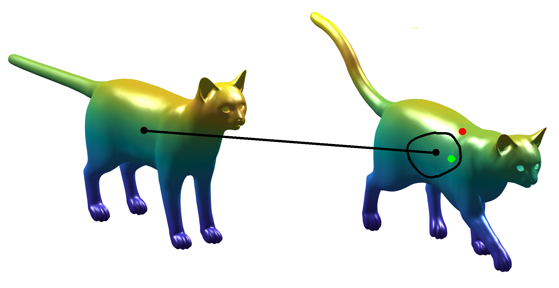
Figure 3: Evaluation of pointwise shape correspondence using the geodesic error. The (correct) ground truth matching is visualised by the black line. On the transformed shape we allow a certain radius of tolerance around the ground truth point. Matchings within the radius (e.g. the green point) are considered to be correct while points outside of the radius (e.g. the red point) are considered as outliers.

As indicated, we are especially interested in run time as well as actual accuracy of the results in context of shape matching. In order to evaluate the accuracy of the methods a dense point-to-point correspondence is performed, involving all vertices the shapes are made off. In detail, the experiments are evaluated as follows.

Discrete Feature Descriptor

The discrete version of the feature descriptor (6) is generated by numerical time integration of the underlying PDE. Therefore, the time axis $[0,t_{M}]$ is subdivided using $(M+1)$-time levels in $0\mathrel{\mathop{\mathchar 58\relax}}=t_{0}<t_{1}<\dots<t_{M}$ and the discrete feature descriptors have the form

$$\mathbf{f_{x_{i}}}=\big{(}u(x_{i},t_{0}),\ldots,u(x_{i},t_{M})\big{)}^{\top}\in\mathbb{R}^{M+1}$$ (66)

for $i=1,\dots,N$. The computation of a discrete feature descriptor at $x_{i}$ for a given shape requires to solve $M$ sparse linear systems of size ${N\times N}$. In total, the computation of all $\mathbf{f}_{x_{i}}$ implies that one has to solve in the total $N\cdot M$ linear systems for each shape.

Hit Rate

The percentage Hit Rate is defined as
$TP/(TP+FP)$, where TP and FP are the number of true positives and false positives, respectively.

Geodesic Error

For the evaluation of the correspondence quality, we followed the Princeton benchmark protocol Kim2011 . This procedure evaluates the precision of the computed matchings $x_{i}$ by determining how far are those away from the actual ground-truth correspondence $x^{*}$. Therefore, a normalised intrinsic distance
$d_{\mathcal{M}}(x_{i},x^{*})/\sqrt{A_{\mathcal{M}}}$ on the transformed shape is introduced. Finally, we accept a matching to be true if the normalised intrinsic distance is smaller than the threshold $0.25$, as illustrated in Figure 3.

Dataset

For the experimental evaluation, datasets at two different resolutions are compared, namely small and large. The small ($N=4344$) shapes of the wolf are taken from the TOSCA dataset TOSCA . The baby shapes have a large resolution ($N=59727$) and are taken from the KIDS dataset KIDS . The datasets are available in the public domain, examples of it are shown in Figure 4. All shapes provide ground-truth, and degenerated triangles were removed.

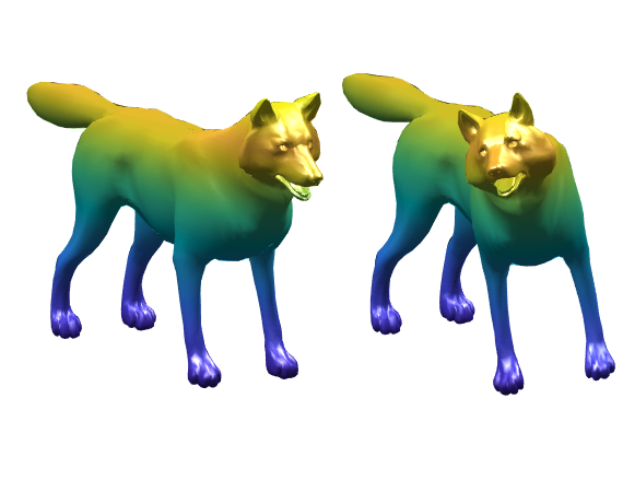
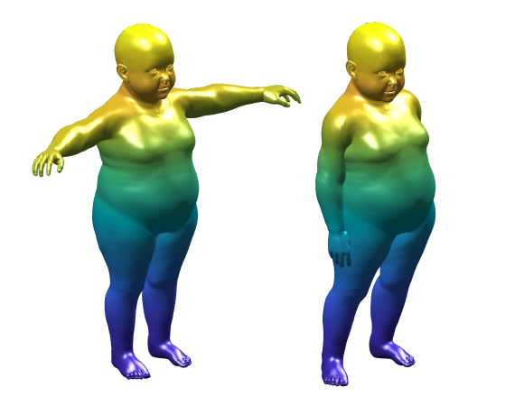
Wolf	Baby
$N=4344$	$N=59727$

Figure 4: For experimental evaluation, shapes at two different resolutions are compared, namely small and large. These are represented by the “wolf" and “baby" , taken from the TOSCA and KIDS dataset, respectively.

General Parameters

We consider $M=25$ time levels such that the corresponding stopping time and the equidistant time increment are fixed to $t_{M}=25$ seconds and $\tau=1$ second, respectively. The parameters are chosen without a fine-tuning, since we are interested to figure out the differences of the numerical methods compared to accuracy and computational costs.

Another issue by using time integration methods is the choice of the initial condition $u(x,0)=u_{0}(x)$. As mentioned in Section 4.2, we apply in this work a discrete delta peak in form of

$$\mathbf{u_{i,0}}=(0,\dots,0,|\Omega_{i}|^{-1},0,\dots 0)^{\top}$$ (67)

For constructing the Krylov subspace $V=\mathcal{K}_{q}((L-\sigma I)^{-1},(L-\sigma I)^{-1}\mathbf{u_{i,0}})$, the expansion point is fixed to $\sigma=0.1$ without loss of generality.

All experiments were done in MATLAB R2018b with an Intel Xeon(R) CPU E5-2609 v3 CPU. The computed eigenvalues and eigenvectors for MCR are computed by the Matlab internal function eigs.

Let us also note that the computations (in this experimental section) were taken by using the Parallel Computing Toolbox integrated in Matlab. As mentioned before, all methods have to solve the geometric heat equation for each point of the given shape independently. This step can be easily parallelised by using the parfor loop to distribute the code to 6 workers here.

7.1 Experimental Results

In what follows, we compare four important numerical approaches at hand of the two selected test datasets.

Results on Sparse Direct Solver

Firstly, we consider the wolf dataset with a small point cloud size of only $N=4344$ points for each of the two shapes, cf. Figure 4. To compute the geodesic error, the geometric heat equation has to be solved numerically once for each point and on each shape. Ultimately, this results in dealing with 217200 linear systems of size ${N\times N}$. By using the LU-decomposition offered by Matlab, the CPU time with around 600s offers significant running costs and is consequently quite inefficient. However, the computational costs can be reduced to around 25s by using the powerful SuiteSparse package, which generates the same geodesic error accuracy.

For the dataset baby, it is necessary to solve 59727 linear systems on each shape and for each time step. In this experiment the direct solver, including SuiteSparse, performs this task in exactly 9267s ($\approx$ 2 1/2 hours). At this point it is recognisable, that large datasets produce high computational costs and that the approach appears to be impractical for such shape matching applications.

In following, the results (CPU time and geodesic error) of the direct solver with the object-oriented factorisation SuiteSparse are used for the comparison of the remaining solvers.

Results on Sparse Iterative Solver

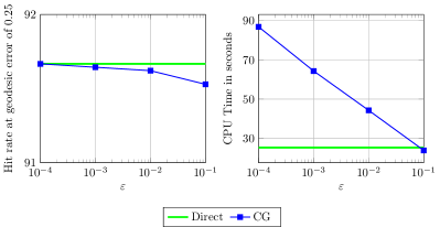
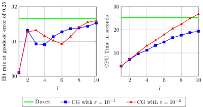
Figure 5: Results on the dataset wolf by using the geometric heat equation. We compare the geodesic error at $0.25$ (left) and the performance time (right) between the direct solver and the CG method for various $\varepsilon$ (top) and different number of CG iterations $l$ (bottom) for $\varepsilon=10^{-1}$ and $\varepsilon=10^{-2}$.

Solving the linear system (34) by using the CG method involves fixing the stopping criterion of the iteration. This involves setting the still free parameter $\varepsilon$ defining accuracy and one may define in addition an upper limit for the number of iterations, compare also our first investigations in BDB-2018 .

Increasing $\varepsilon$ leads to a faster CG approximation, however it turns out that the accuracy remains almost unchanged also for the relatively large value $\varepsilon=10^{-1}$, cf. Figure 5. This means, a good representation of the solution is achieved already after a small number of iterations. In addition, the repeated experiment for $\varepsilon=\{10^{-1},10^{-2}\}$ and various maximum numbers $l$ of CG iterations (i.e. the iterative scheme terminates if one of the conditions is satisfied) is also shown in Figure 5. In this case, the reduction of $l$ only has a minor effect on the geodesic error accuracy, yet it leads to a fast CPU time of only a few seconds.

Regarding the baby dataset the matrix size should be taken into account. A typical problem of large systems is that the convergence becomes slower due to the increase of the condition number of the system matrix, which is due to a larger system size. Therefore, we apply the PCG method including the modified incomplete Cholesky (MIC) factorisation as a preconditioner, which is a modern variation of the standard incomplete Cholesky (IC) decomposition and possesses in general a better performance. The mentioned factorisation uses a parameter-dependent, numerical fill-in strategy MIC($\gamma$), where the parameter $\gamma$ is called drop tolerance and describes a dropping criterion for matrix entries, cf. Saad2003 . In practice cf. Benzi2002 ; Baehr2017 , good results are obtained for values of $\gamma\in[10^{-4},10^{-2}]$, such that we fixed $\gamma=10^{-3}$.

The results for MIC($10^{-3}$) are shown in Figure 6. Compared to the performance of the direct solver no improvement is achieved. Furthermore, a closer examination of the required iterations for the termination of the iterative algorithm shows that PCG needed just about 1 iteration. Therefore, PCG cannot be tuned further with regard to its performance. The latter observation again inspires the idea to perform the CG method for a very small number of iterations $l\leq 10$, which accordingly should be sufficient to gain acceptable results in fast CPU time; see also our previous study BDB-2018 compared to which we present here some refinements of the results. The results of CG for $\varepsilon=10^{-1}$ and small numbers $l$ of CG iterations are shown in Figure 6. Also in this case, the iterative solver can reduce the computational effort significantly up to 80%, however the percentage deviation of the accuracy in relation to the direct solver is approximately up to 10%.

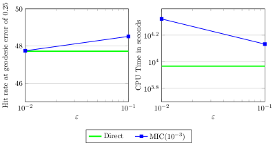
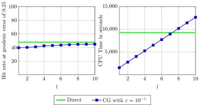
Figure 6: Results on the dataset baby by using the geometric heat equation. We compare the geodesic error at $0.25$ (left) and the performance time (right) between the direct solver and the PCG method, including MIC$(10^{-3})$, for various $\varepsilon$ (top). In addition, we present a comparison between the direct method and the CG method (bottom) for $\varepsilon=10^{-1}$ and the first ten CG iterations $l$. The latter means, the iterative scheme terminates if one of the conditions is satisfied.

Krylov Subspace Model Order Reduction

The results of KSMOR for the wolf dataset are illustrated in Figure 7. Increasing the dimension of Krylov subspaces $q$ leads as expected, to a more accurate approximation, whereby the same geodesic error accuracy compared to the direct solver can already be achieved for $q\leq 10$. The required computational costs correspond to those of CG, however we obtain a higher accuracy in terms of the geodesic error.

The same performance output is obtained by applying KSMOR for the baby dataset. Also for this dataset, using already approximately $q=2$ is deemed to be sufficient to obtain an excellent trade-off between quality and efficacy and can save around 95% of the computational time in relation to the direct solver. However, the running time for $q=2$ with around 450 seconds is still significant for this standard size shape.

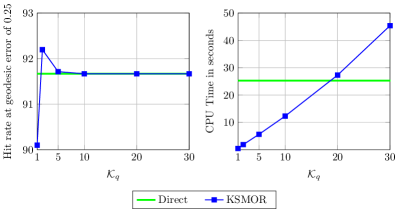
Figure 7: Results on the dataset wolf by using the geometric heat equation. We compare the geodesic error at $0.25$ (left) and the performance time (right) between the direct solver and KSMOR method for a different number of Krylov subspaces $\mathcal{K}_{q}$.

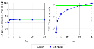
Figure 8: Results on the dataset baby by using the geometric heat equation. We compare the geodesic error at $0.25$ (left) and the performance time (right) between the direct solver and KSMOR method for a different number of Krylov subspaces $\mathcal{K}_{q}$.

Modal Coordinate Reduction (MCR)

Finally, we explore the MCR technique. The whole MCR process and reported computational times includes the computation of eigenvalues, eigenvectors and solving of the subsequently reduced systems. For the experiments we increase the number of used ordered modes, starting from $N_{max}=5$ and going up to $N_{max}=3000$. Regarding to the wolf dataset we would expect that the correspondence quality gets better when increasing the number of modes. However, the evaluation in Figure 9 does not show this desirable behaviour. The outcome for a small spectrum $N_{\max}\approx 10$ are much better than for a large spectrum $N_{\max}\approx 1000$, which seems at first glance not intuitive. The geodesic error oscillates in the range of $N_{max}\in[20,1000]$, and beginning from about $N_{max}=2000$ which is a high number of modes for the approach it converges against the solution of the direct method. Nevertheless, let us stress that the CPU time is incredibly fast when using a small number of modes. For values up to ${N_{max}=100}$ the approximate solution is computed in less than 1 second, however the obtained geodesic error accuracy is not too high.

Applying the MCR technique to the baby dataset yields in the total a similar behaviour, but we also observe a surprising result, see Figure 10. In this experiment again, a small spectrum leads to better results compared to larger numbers of modes. In contrast to the wolf dataset, two striking observations can be made. First, using $N_{max}=[5,10]$ even outperforms the geodesic error accuracy in relation to the direct solver and secondly the geodesic error of both solvers are nearly equal already for $N_{max}=50$. In this case, MCR has an extremely short running time of around 10 seconds, which reduces the computational effort compared to the direct solution by around 99.999%.

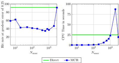
Figure 9: Results on the dataset wolf by using the geometric heat equation. We compare the geodesic error at $0.25$ (left) and the performance time (right) between the direct solver and the MCR technique for different number of modes $N_{\max}\in[5,3000]$.

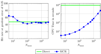
Figure 10: Results on the dataset baby by using the geometric heat equation. We compare the geodesic error at $0.25$ (left) and the performance time (right) between the direct solver and the MCR technique for different number of modes $N_{\max}\in[5,3000]$.

Discussion of Solvers

The experiments illustrated the performances of all applied solvers. The direct solver produces the best results in relation to the geodesic error accuracy. However, for high resolution shapes ($N>50000$) the method is quite inefficient and generates computational costs amounting to several hours.

The CG method may reduce the computational costs by around 80%, whereby the percentage deviation of the accuracy in relation to the direct method is approximately less than 10%.

Applying the KSMOR method achieves an even better performance. In this study, the choice of just $q=2$ saves around 95% of the computational time, whereby the percentage deviation of the geodesic error accuracy in relation to the direct solver is only around 1%.

The computational costs of the MCR method grow exponentially (by increasing $N_{max}$) and accordingly a practicable value $N_{max}$ should be small. It is remarkable that the results for a small spectrum ($N_{max}\approx 10$) are similar or even better to the ones for a significantly larger spectrum ($N_{max}\approx 1000$). In case of a small spectrum, the MCR method is highly efficient and can save around 99% CPU time, which suggests that this technique is favourable for solving shape matching by time integration.

Due to the incredible power of MCR, subsequently we follow this technique within this paper. Moreover, an interesting aspect would be to tune the method so that it becomes more stable when using it with shapes such as the wolf shape, and in addition to improve the performance of the time integration approach.

Let us stress that we selected the two datasets used above since they are useful for demonstrating in detail the described behaviour of the schemes as it can be observed in all tests we performed. They show the typical range of results that one obtains in terms of quality and efficiency.

8 Optimised Numerical Signatures

As a result of the last section, the MCR method appears favourable for computing the numerical shape signature, especially when considering the extremely low computational costs. However, the geodesic error accuracy seems to depend on the given shapes and also on the number of used modes. For this reason, the computation of the MCR signature leads to new challenges, as the aim is to ensure in a reliable way a high quality of results without additional computational costs.

In the following, we introduce several means in order to enhance robustness and quality. In doing this, we significantly extend our previous conference paper BDB-2018 as already indicated.

8.1 Improved Eigenvalue Computation

An important aspect of the MCR method is the way how to compute the eigenvalues $\lambda$ and eigenvectors $\mathbf{v}$ of the system matrix $L=D^{-1}W$. As described in Section 6.1, the computation is performed by solving the generalised eigenvalue problem (47), which uses certain properties of the underlying matrices $D$ and $W$ to produce numerically real-valued eigenvalues and eigenvectors. However, the computation in this way may exhibit traces of instability in numerical practice.

Another more favourable approach is to transform the generalised eigenvalue problem $W\mathbf{v}=\lambda D\mathbf{v}$ into the standard eigenvalue problem without loss of the symmetry of $W$, such that more robust numerical eigensolvers can be applied. The symmetric standard eigenvalue problem can be achieved by a similarity transformation in the following way

$$L=D^{-1}W=D^{-\frac{1}{2}}D^{-\frac{1}{2}}WD^{-\frac{1}{2}}D^{\frac{1}{2}}=D^{-\frac{1}{2}}BD^{\frac{1}{2}}$$ (68)

whereby the matrix $B=D^{-\frac{1}{2}}WD^{-\frac{1}{2}}$ is symmetric due to the symmetry of $W$. Thus, the matrices $L$ and $B$ are similar and have the same real eigenvalues. Moreover, the eigenpair $(\lambda,\mathbf{v})$ of $B\mathbf{v}=\lambda\mathbf{v}$ corresponds to the eigenpair $(\lambda,\mathbf{\widetilde{v}})=(\lambda,D^{-\frac{1}{2}}\mathbf{v})$ of $L\mathbf{\widetilde{v}}=\lambda\mathbf{\widetilde{v}}$. The matrix $D^{-\frac{1}{2}}$ in (68) is well-defined due to the positive diagonal matrix $D^{-1}$ and is consequently also positive diagonal. The eigenvectors $\mathbf{v}$ of $B$ are orthonormal with $\mathbf{v_{i}}^{\top}\mathbf{v_{j}}=\delta_{i,j}$ so that the eigenvectors of $L$ are $D$-orthogonal

$$\mathbf{v_{i}}^{\top}\mathbf{v_{j}}=(D^{\frac{1}{2}}\mathbf{\widetilde{v}_{i}})^{\top}D^{\frac{1}{2}}\mathbf{\widetilde{v}_{j}}=\mathbf{\widetilde{v}_{i}}^{\top}D\mathbf{\widetilde{v}_{j}}=\delta_{i,j}$$ (69)

Let us briefly comment on an important issue here that may arise when adapting our framework to different types of spatial discretisations such as e.g. the quite prominent finite element method which is one of the frequently used methods for numerical computations. The proposed transformation is applicable whenever $D^{-1}$ (or $D$) is symmetric positive definite. This situation will for instance occur when using the finite element ansatz instead of the presented finite volume set-up in Section 4.2, whereby $D^{-1}$ consequently represents the mass matrix in that setting cf. Zhang2010 . In this case, the generalised eigenvalue problem $W\mathbf{v}=\lambda D\mathbf{v}$ can be reformulated by using the existing Cholesky decomposition $D=LL^{\top}$, with a lower triangular matrix $L$ and positive diagonal entries, as

$$W\mathbf{v}=\lambda D\mathbf{v}$$

$$\Leftrightarrow\quad W\mathbf{v}=\lambda LL^{\top}\mathbf{v}$$

$$\Leftrightarrow\quad L^{-1}W\mathbf{v}=\lambda L^{\top}\mathbf{v}$$

$$\Leftrightarrow\quad L^{-1}WL^{-\top}L^{\top}\mathbf{v}=\lambda L^{\top}\mathbf{v}$$

$$\Leftrightarrow\quad L^{-1}WL^{-\top}\mathbf{\widetilde{v}}=\lambda\mathbf{\widetilde{v}}$$

$$\Leftrightarrow\quad B\mathbf{\widetilde{v}}=\lambda\mathbf{\widetilde{v}}$$ (70)

with $B=L^{-1}WL^{-\top}$ and $\mathbf{\widetilde{v}}=L^{\top}\mathbf{v}$. The eigenvectors are then retransformed according to $\mathbf{v}=L^{-\top}\mathbf{\widetilde{v}}$. Clearly, for a diagonal matrix as in our method holds $D=D^{\frac{1}{2}}D^{\frac{1}{2}}$ so that (70) corresponds to (68).

In the following, we analyse the abovementioned computation of the eigenpairs $(\lambda,\mathbf{v})$ using the wolf and baby dataset. The evaluation by solving the generalised and the symmetric eigenvalue problem is presented in Figure 11. As we indicated above, we observe that the ansatz of using the similarity transformation for tackling the eigenvalue problem achieves significantly more stable matching results. Let us emphasise that we see in the case of the wolf shape after this improvement the accuracy behaviour that we would have expected when increasing the number of modes which indicates the better robustness of the approach, and also for the baby shape we obtain a quality improvement.

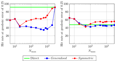
Figure 11: Results on the dataset wolf (left) and baby (right) by using the geometric heat equation. We compare the geodesic error at $0.25$ between the direct solver and the MCR technique for different number of modes $N_{\max}\in[5,3000]$. The eigenvalues and eigenvectors are computed by solving the generalised and the symmetric eigenvalue problem. Using the similarity transformation achieves more stable matching results.

8.2 Improved Scaling of the Integration Domain $[0,\mathit{t_{M}}]$

We also discuss now the impact of the choice of the parameter $t_{M}$ with respect to the MCR technique. The computed numerical signatures are computed over a temporal domain $(0,t_{M}]$, which makes them easily measurable for the shape matching purposes.

Let us start our discussion of time scaling by considering some ideas for motivation. It is well-known, that the analytic solution of the semi-discrete geometric heat equation $\mathbf{\dot{u}}=L\mathbf{u}$ has the form

$$\mathbf{u}(t)=e^{Lt}\mathbf{u}(0)=e^{V\Lambda V^{\top}Dt}\mathbf{u}(0)=Ve^{\Lambda t}V^{\top}D\mathbf{u}(0)$$ (71)

or more precisely

$$\mathbf{u}(t)=\sum_{i=1}^{N}e^{\lambda_{i}t}\mathbf{v_{i}}\mathbf{v_{i}}^{\top}D\mathbf{u}(0)=\sum_{i=1}^{N}\mathbf{v_{i}}^{\top}D\mathbf{u}(0)e^{\lambda_{i}t}\mathbf{v_{i}}$$ (72)

where $\mathbf{v_{i}}^{\top}D\mathbf{u}(0)$ is a scalar. Therefore, the pointwise feature descriptor has the form

$$f_{x_{j}}(t)\mathrel{\mathop{\mathchar 58\relax}}=u(x,t)_{\mid_{x=x_{j}}} =\Big{(}\sum_{i=1}^{N}\mathbf{v_{i}}^{\top}D\mathbf{u_{j}}(0)e^{\lambda_{i}t}\mathbf{v_{i}}\Big{)}^{\top}\mathbf{\hat{e}_{j}}$$

$$=\Big{(}\sum_{i=1}^{N}\mathbf{v_{i}}^{\top}\mathbf{\hat{e}_{j}}e^{\lambda_{i}t}\mathbf{v_{i}}\Big{)}^{\top}\mathbf{\hat{e}_{j}}$$ (73)

with $D\mathbf{u_{j}}(0)=\mathbf{\hat{e}_{j}}$, where $\mathbf{\hat{e}_{j}}$ is the $j$-th unit vector. The representation of the solution (73) describes an exponential decay of heat transferred away from the considered point $x_{j}$. Using only a small number of $r$ dominant frequencies (small eigenvalues) of a system, the reduced basis solution as approximative feature descriptor is given by

$$f_{x_{j}}(t)\approx\widetilde{u}(x_{j},t)=\Big{(}\sum_{i=1}^{r}\mathbf{v_{i}}^{\top}\mathbf{\hat{e}_{j}}e^{\lambda_{i}t}\mathbf{v_{i}}\Big{)}^{\top}\mathbf{\hat{e}_{j}}$$ (74)

Furthermore, the reduced solution (74) with eigenvalues $0<\mathinner{\!\left\lvert\lambda_{i}\right\rvert}\ll 1$ ($i=1,\ldots,r$), can be simplified for small times $t$ as

$$\widetilde{u}(x_{j},t) =\Big{(}\sum_{i=1}^{r}\mathbf{v_{i}}^{\top}\mathbf{\hat{e}_{j}}\underbrace{e^{\lambda_{i}t}}_{\approx 1}\mathbf{v_{i}}\Big{)}^{\top}\mathbf{\hat{e}_{j}}$$

$$\approx(V{\mathbf{y_{j}}})^{\top}\mathbf{\hat{e}_{j}}=c_{j}$$ (75)

for all time levels $t=t_{k}$, where $c_{j}$ is a constant and ${\mathbf{y_{j}}}$ is the $j$-th column vector of $V^{\top}$.

After this brief discussion, let us now turn again to the MCR method. The analogous representation as above is described in MCR which is based on dominant modes (low frequencies). The solution of the reduced model $\dot{\mathbf{w}}(t)=\Lambda_{r}\mathbf{w}(t)$ of order $r$ is given by

$$\mathbf{w}(t)=\underbrace{e^{\Lambda_{r}t}}_{\approx I}\mathbf{w}(0)\approx\mathbf{w}(0)$$ (76)

so that with $\mathbf{u}(t)\approx V_{r}\mathbf{w}(t)$ follows

$$\mathbf{u}(t)\approx V_{r}\mathbf{w}(t)=V_{r}\mathbf{w}(0)=V_{r}V_{r}^{\top}D\mathbf{u}(0)$$ (77)

Consequently, the pointwise MCR feature descriptor results in

$$f_{x_{j}}(t) \approx\bigl{(}V_{r}V_{r}^{\top}D\mathbf{u}(0)\bigr{)}^{\top}\mathbf{\hat{e}_{j}}$$

$$=\bigl{(}V_{r}V_{r}^{\top}\mathbf{\hat{e}_{j}}\bigr{)}^{\top}\mathbf{\hat{e}_{j}}=\left(V_{r}\mathbf{y_{r,j}}\right)^{\top}\mathbf{\hat{e}_{j}}=c_{r,j}$$ (78)

Having in mind the approximately constant behaviour of the approximative solution (75) and comparing this with (78) shows that the MCR descriptor exhibits in general a slow rate of heat transfer. Let us note that this shows that the MCR shape signature is not highly precise in terms of the indicated geometric location on a shape, especially when using a small number of modes as shown for $f_{x_{1}}(t)$ in Figure 12.

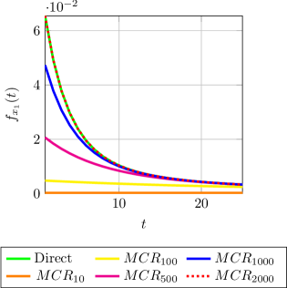
Figure 12: Results on the dataset wolf by using the geometric heat equation for $t_{M}=25$. We compare the discrete feature descriptor $f_{x_{1}}(t)$ obtained by the direct solver and the MCR technique for different number of modes $N_{\max}$, shortened here as $MCR_{N_{\max}}$. Obviously, a small number of used modes (here $N_{\max}=10$ or $N_{\max}=100$) correlate to a slow rate of heat transfer. Therefore, the feature descriptors tend to almost constant functions when decreasing the number of modes, and this may lead to shape signature values that give not much information about the geometry of the given surface.

This observation requires an appropriate adaptation of the MCR method concerning the computation of the feature descriptor in (76)-(78). An useful way to enhance without too much computational effort the geometric information for the shape matching process is to modify the numerical signatures via an adapted temporal domain. As we will find, an adapted time $t^{\star}$ with $t^{\star}\gg t_{M}$ for small eigenvalues $0<\mathinner{\!\left\lvert\lambda_{i}\right\rvert}\ll 1$ causes $e^{\lambda_{i}t^{\star}}\ll e^{\lambda_{i}t_{M}}\approx 1$. Let us explain, that we have $\lambda_{i}\leq 0$, so that the latter inequality bears the meaning that we obtain by rescaling time in the indicated way a more significant spreading of values, so that the eigenvalues are more discriminative. This improves the physical characteristics and consequently the diversity of the MCR signatures.

Let us begin with the following thoughts. Obviously, the rate of heat transfer of the reduced feature descriptor of order $r$ depends on the fastest mode ${\lambda_{r}}$. Moreover, a higher order reduced model $r^{\prime}>r$ corresponds to faster heat transfer, which in turn implies $t^{\star}_{r^{\prime}}<t^{\star}_{r}$ to be suitable in order to get a more discriminative descriptor value. Based on these considerations, we will modify $[0,\mathit{t_{M}}]$ to $[0,\mathit{t^{\star}}]$ in the following way.

We propose to adapt the temporal domain in a simple way by the function

$$t^{\star}(\lambda_{r})=\frac{k}{\sqrt{\mathinner{\!\left\lvert\lambda_{r}\right\rvert}}}$$ (79)

where $k$ is a constant. This still to be determined parameter is defined in our construction via the condition

$$t_{M}\stackrel{{\scriptstyle!}}{{=}}t^{\star}(\lambda_{N})=\frac{k}{\sqrt{\mathinner{\!\left\lvert\lambda_{N}\right\rvert}}}$$ (80)

which must be fulfilled for the reduced model of full order $N$. Therefore, making use of (80) the modified integration domain $[0,\mathit{t^{\star}(\lambda_{r})}]$ is specified by

$$t^{\star}(\lambda_{r})=\frac{t_{M}\sqrt{\mathinner{\!\left\lvert\lambda_{N}\right\rvert}}}{\sqrt{\mathinner{\!\left\lvert\lambda_{r}\right\rvert}}}$$ (81)

The corresponding time increment is easily calculated via $\tau=\frac{t^{\star}}{M}$. One may notice, that the square root prevents an extremely large time domain (eigenvalues $\mathinner{\!\left\lvert\lambda_{r}\right\rvert}$ grow exponentially) which would lead anew to less descriptive shape signatures.

As an example for illustrating the usefulness of our rescaling, the mentioned strategy yields for the wolf dataset the modified integration domain $[0,\mathit{t^{\star}}]$ shown in Figure 13.

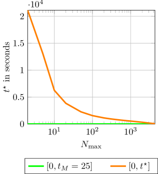
Figure 13: Results on the dataset wolf by using the geometric heat equation. Visualisation of the original $[0,\mathit{t_{M}}=25]$ and the adapted $[0,\mathit{t^{\star}}]$ temporal domain using the formula (81) for a different number of modes $N_{\max}\in[2,4344]$.

Based on this modification the adapted feature descriptor $f_{x_{1}}(t)$, illustrated in Figure 14, demonstrates a more suitable numerical signature.

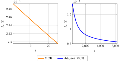
Figure 14: Results on the dataset wolf by using the geometric heat equation for $M=25$ time levels. We compare the discrete feature descriptor $f_{x_{1}}(t)$ between the original $[0,\mathit{t_{M}}=25]$ and the adapted $[0,\mathit{t^{\star}}]$ temporal domain using the formula (81) computed by the MCR technique for $N_{\max}=10$. Note that the left figure shows a nearly constant function whereas a decaying exponential function as on the right after rescaling is the desired result. Clearly, the modified integration domain yields a more suitable numerical signature.

Finally, we compare the performances of the MCR technique including the similarity transformation by using the original $[0,\mathit{t_{M}}=25]$ and the adapted $[0,\mathit{t^{\star}}]$ temporal domain for the given datasets. The corresponding visualisation of the evaluation is presented in Figure 15.

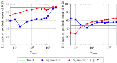
Figure 15: Results on the dataset wolf (left) and baby (right) by using the geometric heat equation. We compare the geodesic error at $0.25$ between the original $[0,\mathit{t_{M}}=25]$ and the adapted $[0,\mathit{t^{\star}}]$ temporal domain using formula (81) computed by the MCR technique for different number of modes $N_{\max}\in[5,3000]$. The eigenvalues and eigenvectors are constructed by using the similarity transformation.

In general, the substantial increase of the stopping time $t^{\star}(\lambda_{r})$ of the reduced model improves the geodesic error accuracy. However, the results may differ for a small spectrum as in the case of the baby dataset. A possible heuristic explanation could be based on the nature of the first few modes that correspond to a low pass filtered shape signature, meaning that one may obtain a good matching of a coarse shape representation in some cases.

In what follows, we will denote the solver including both abovementioned improvements as optimised MCR method.

8.3 Implementation of the Optimised MCR Heat Signature

We now describe briefly the simple implementation of the MCR signature which makes it a candidate for practical shape analysis purposes.

As already mentioned, the feature descriptors have to be computed for each point and on each shape. Nevertheless, the computation of the MCR signatures can be done simultaneously for all locations $x_{i}\in\mathcal{M}$ on a given shape by putting it into the format of a matrix-vector-multiplication, which additionally improves the computational efficiency.

To this end, solving the geometric heat equation by (56) can be reformulated as

$$W^{k}= PW^{k-1},\quad W^{0}=V_{r}^{\top}DU^{0}=V_{r}^{\top}$$ (82)

with $V_{r}\in\mathbb{R}^{N\times r}$, $W\in\mathbb{R}^{r\times N}$ and $U^{0}=D^{-1}$ due to $\mathbf{u_{i}}(0)=(0,\dots,0,|\Omega_{i}|^{-1},0,\dots 0)^{\top}$. The algorithm for computing the optimised MCR heat signature is described in Figure 16. Let us note that the extraction of the feature descriptors $f_{x_{i}}$ in step 3d) of the algorithm is based on the Hadamard product. Finally, the correspondence quality can be evaluated based on the selected measure.

Let us mention, incidentally, the computation of the temporal domain $[0,\mathit{t^{\star}}]$ and the time increment $\tau$ in step 2 of the described algorithm is only done for the reference shape. This ensures to perform a correct matching by comparing the feature descriptors for different locations $x_{i}\in\mathcal{M}$ and $\widetilde{x}_{j}\in\widetilde{\mathcal{M}}$ on the same scale.

Algorithm 1 Computation of MCR Heat Signature

0:  Matrices $D^{-1},W$, reduction parameter $r$, amount of time levels $M$, stopping time $t_{M}$

0:  $\mathbf{f_{x_{i}}}$ Reference Shape

  1. Computation of $\Lambda_{r}\in\mathbb{R}^{r\times r}$ and $V_{r}\in\mathbb{R}^{N\times r}$

  a) Compute $r$ dominant eigenpairs $(\lambda,\mathbf{v})$ of $B=D^{-\frac{1}{2}}WD^{-\frac{1}{2}}$ by solving $B\mathbf{v}=\lambda\mathbf{v}$

  b) Calculation of $(\lambda,\mathbf{\widetilde{v}})$ of $L$ with $\mathbf{\widetilde{v}}=D^{-\frac{1}{2}}\mathbf{v}$

  2.) Computation of $[0,\mathit{t^{\star}}]$ using (81)

  a) Compute fastest mode $\lambda_{N}$ by solving $B\mathbf{v}=\lambda\mathbf{v}$

  b) Calculate $t^{\star}(\lambda_{r})=\displaystyle{\frac{t_{M}\sqrt{\mathinner{\!\left\lvert\lambda_{N}\right\rvert}}}{\sqrt{\mathinner{\!\left\lvert\lambda_{r}\right\rvert}}}}$, $\tau=\displaystyle{\frac{t^{\star}}{M}}$

  3.) Solving reduced system (82)

  a) Set $W^{0}=V_{r}^{\top}$

  b) Compute $P=(I-\tau\Lambda_{r})^{-1}$

  c) Solve $W^{k}=PW^{k-1}$ for $k=1,\ldots,M$

  d) Extract $\mathbf{f_{x_{i}}}$ by $f_{x_{i}}(t_{k})=\sum\limits_{j=1}^{r}[(V_{r}\circ(W^{k})^{\top})]_{ij}$ for $k=1,\ldots,M$ Transformed ShapeRepeat computations of Steps 1. and 3.

Figure 16: Algorithm for computing the optimised MCR signature by solving the geometric heat equation. The procedure is analogously applicable to the geometric wave equation.

8.4 Optimised MCR Wave Signature

The abovementioned aspects can also be used to solve the geometric wave equation numerically by the MCR technique. However, based on our experiments we propose to define the modified integration domain $[0,\mathit{t^{\star}(\lambda_{r})}]$ in the following way

$$t^{\star}(\lambda_{r})=\frac{t_{M}\sqrt[4]{\mathinner{\!\left\lvert\lambda_{N}\right\rvert}}}{\sqrt[4]{\mathinner{\!\left\lvert\lambda_{r}\right\rvert}}}$$ (83)

The implementation (cf. Figure 16) for computing the optimised MCR wave signature remains identical to the algorithm presented above, except for the calculation of $t^{\star}(\lambda_{r})$ and for solving the reduced system in Step 2b) and Step 3, respectively. The modifications in Step 3 are the following:

• Compute $P=(I-\tau^{2}\Lambda_{r})^{-1}$
  

• Solve $W^{1}=PW^{0}$ and $W^{k}=P(2W^{k-1}-W^{k-2})$ for $k=2,\ldots,M$

For completeness the results of the standard and optimised MCR wave signatures for the given datasets are presented in Figure 17. Moreover, a comparison of the optimised MCR method by using the geometric heat and wave equation is illustrated in Figure 18.

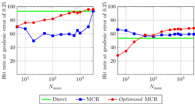
Figure 17: Results on the dataset wolf (left) and baby (right) by using the geometric wave equation. We compare the geodesic error at $0.25$ between the original $[0,\mathit{t_{M}}=25]$ and the adapted $[0,\mathit{t^{\star}}]$ temporal domain using formula (83) computed by the MCR technique for different number of modes $N_{\max}\in[5,3000]$. The eigenvalues and eigenvectors of the original and optimised MCR are constructed by solving the generalised and symmetric eigenvalue problem, respectively.

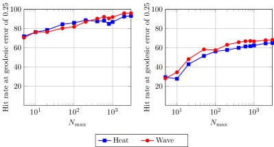
Figure 18: Results on the dataset wolf (left) and baby (right) by applying the optimised MCR technique. We compare the geodesic error at $0.25$ between using the geometric heat and wave equation for different number of modes $N_{\max}\in[5,3000]$.

9 Reference Model: Spectral Methods

The spectral methods of the heat kernel signature (HKS) and the wave kernel signature (WKS) that we employ for comparison with our approach are based on the geometric heat equation SOG and the geometric Schrödinger equation ASC , respectively. Let us note here, that also the process described in MORCC is technically related to our appraoch as it is a time evolution method and based on diffusion. However, as already noted in MORCC , the technique is computationally very demanding compared to HKS and WKS construction. Thus we refrain from comparing to this method since one of our main aims is computational efficiency.

For constructing spectral descriptors, it is assumed that the solution of both equations will take the form $u(x,t)=\phi(x)\theta(t)$ due to the fact that the underlying PDEs are linear and homogeneous. This approach works because if the product of two functions $\phi$ and $\theta$ of independent variables $x$ and $t$ is a constant, each function must separately be a constant. Therefore, one may separate the equations to get a function of only $t$ and $x$, respectively:

$$\kappa\dfrac{\partial_{t}\theta(t)}{\theta(t)}=\dfrac{\Delta_{\mathcal{M}}\phi(x)}{\phi(x)}=\text{const}=-\lambda$$ (84)

where $\kappa$ summarises both equations ($\kappa=1$ for geometric heat equation, $\kappa=i$ for geometric Schrödinger equation), and $-\lambda$ is called the separation constant which is arbitrary for the moment. This leaves us with two new equations, namely an ODE for the temporal component

$$\partial_{t}\theta(t)=-\kappa\lambda\theta(t),\quad t\in[0,T]$$ (85)

and the spatial part takes the form of the Helmholtz equation

$${\begin{cases}\Delta_{\mathcal{M}}\phi(x)=-\lambda\phi(x),&{\mbox{}}x\in\mathcal{M}\\ \langle\nabla_{\mathcal{M}}\phi,n\rangle=0,&{\mbox{}}x\in\partial\mathcal{M}\end{cases}}$$ (86)

where the constant $\lambda$ has here the meaning of the operator’s eigenvalue.

The Laplace-Beltrami operator is a self-adjoint operator on the space $L_{2}(\mathcal{M})$ (since we assumed the shapes to be compact). This implies that the Helmholtz equation has an infinite number of non-trivial solutions $\phi_{k}$ for certain eigenvalues $\lambda_{k}$ and corresponding eigenfunctions, which is a result of the spectral theorem Sauvigny2012 . Consequently, (86) takes on the format

$${\begin{cases}\Delta_{\mathcal{M}}\phi_{k}(x)=-\lambda_{k}\phi_{k}(x),&{\mbox{}}x\in\mathcal{M}\\ \langle\nabla_{\mathcal{M}}\phi_{k},n\rangle=0,&{\mbox{}}x\in\partial\mathcal{M}\end{cases}}\quad k=1,2,\ldots$$ (87)

Concerning the ordered spectrum of eigenvalues $0=\lambda_{1}<\lambda_{2}\leq\ldots$ and the corresponding eigenfunctions $\phi_{1},\phi_{2},\ldots$ let us note that the latter form an orthonormal basis of $L_{2}(\mathcal{M})$. Moreover, in case of Neumann boundary conditions (or no shape boundaries) constant functions are solutions of the Helmholtz equation for the first eigenvalue with zero value.

It is well known that the eigenfunctions are a natural generalisation of the classical Fourier basis for working with functions on shapes. Let us also note that the physical interpretation of the Helmholtz equation is the following. The shape of a 3D object can be thought of as a vibrating membrane, the $\phi_{k}$ can be interpreted as its vibration modes whereas $\lambda_{k}$ have the meaning of the corresponding vibration frequencies, sorted from low to high.

For each index $k$ one thus obtains an ODE (16) which can be solved by integration using the indefinite integral:

$$\int\dfrac{\mathrm{d}\theta(t)}{\theta(t)}=-\int\kappa\lambda_{k}\mathrm{d}t\quad\Longrightarrow\quad\theta(t)=\alpha_{k}e^{-\kappa\lambda_{k}t}$$ (88)

where the integration constant $\alpha_{k}$ should satisfy the initial condition of the $k$-th eigenfunction. The final product solution then reads as

$$u_{k}(x,t)=\alpha_{k}e^{-\kappa\lambda_{k}t}\phi_{k}(x)\,$$ (89)

The principle of superposition says that if we have several solutions to a linear homogeneous differential equation then their sum is also a solution. Therefore, a closed-form solution of the geometric heat equation in terms of a series expression can be written as

$$u(x,t)=\sum_{k=1}^{\infty}\alpha_{k}e^{-\lambda_{k}t}\phi_{k}(x)\,$$ (90)

and the solution of the geometric Schrödinger equation reads as

$$u(x,t)=\sum_{k=1}^{\infty}\alpha_{k}e^{-i\lambda_{k}t}\phi_{k}(x)\,$$ (91)

where the coefficients $\alpha_{k}$ are chosen to fulfil the initial condition.

Heat Kernel Signature.

The coefficients $\alpha_{k}$ in our expansion can be computed by using the $L_{2}$ inner product

$$\alpha_{k}=\langle u_{0},\phi_{k}\rangle_{L_{2}(\mathcal{M})}=\int\limits_{\mathcal{M}}u_{0}(y)\phi_{k}(y)\,\mathrm{d}y$$ (92)

such that one may compute

$$u(x,t) =\sum_{k=1}^{\infty}\Bigg{(}\int\limits_{\mathcal{M}}u_{0}(y)\phi_{k}(y)\,\mathrm{d}y\Bigg{)}e^{-\lambda_{k}t}\phi_{k}(x)$$ (93)

$$=\int\limits_{\mathcal{M}}u_{0}(y)\underbrace{\bigg{(}\sum_{k=1}^{\infty}e^{-\lambda_{k}t}\phi_{k}(y)\phi_{k}(x)\bigg{)}}_{=K(x,y,t)}\,\mathrm{d}y\,$$ (94)

The heat kernel $K(x,y,t)$ describes the amount of heat transmitted from $x$ to $y$ after time $t$. By setting the initial condition to be a delta heat distribution with $u_{0}(y)=\delta_{x}(y)$ at the position $y$, we thus obtain according to SOG the heat kernel signature

$$\text{HKS}(x,t)=\sum_{k=1}^{\infty}e^{-\lambda_{k}t}\left|\phi_{k}(x)\right|^{2}\,$$ (95)

where the shifting property of the delta distribution $f(x)=\int_{\mathcal{M}}f(y)\delta_{x}(y)\,\mathrm{d}y$ was used. In accordance, the quantity $\text{HKS}(x,t)$ describes the amount of heat present at point $x$ at time $t$.

Wave Kernel Signature.

The WKS ASC is defined to be the time-averaged probability of detecting a particle of a certain energy distribution at the point $x$, formulated as

$$\text{WKS}(x,t) =\lim\limits_{T\rightarrow\infty}\dfrac{1}{T}\int\limits_{0}^{T}|u|^{2}\mathrm{d}t=\sum\limits_{k=1}^{\infty}\left|\alpha_{k}\right|^{2}\left|\phi_{k}(x)\right|^{2}\,$$ (96)

Furthermore, $\alpha_{k}=\alpha(e_{k})$ becomes a function of the energy distribution $e_{k}$ of the quantum mechanical particle and can be chosen as a log-normal distribution, i.e.

$$\left|\alpha_{k}\right|^{2}=\exp\bigg{(}\frac{-(e-\log\lambda_{k})^{2}}{2\sigma^{2}}\bigg{)}\,$$ (97)

where the variance of the energy distribution is denoted by $\sigma$, see again ASC for more details.

The eigenfunctions and eigenvalues of the discrete Laplace-Beltrami operator are computed by performing the generalised eigendecomposition

$$L\phi_{k}=-\lambda_{k}\phi_{k}\,,\quad k=1,\ldots,N\,$$ (98)

10 Experimental Results: Optimised MCR vs. Kernel-based Methods

In the following, we give a detailed quantitative evaluation of the proposed MCR technique compared to the kernel-based methods. In the total, we will compare the developed optimised MCR techniques relying on both geometric heat and wave equation, respectively, with HKS and WKS. To this end, we benchmark the methods at hand of the complete TOSCA dataset whose shapes are almost isometric.

Let us note again, that the comparison of the optimised MCR wave signature and WKS is not based on the same PDE model although the latter notion (wave kernel signature) suggests this, as the latter method is based on the Schrödinger equation. Concerning this point, let us note first that a recent work DBH-2017 has shown that the numerical descriptor based on the geometric wave equation gains better results than the numerical descriptor based on the geometric Schrödinger equation. Secondly, within the class of kernel-based methods the WKS can be considered as a competitive descriptor. Therefore, we compare the optimised MCR wave signature in its relation to the WKS due to their distinct role in their respective class.

Evaluation Measure.

The correspondence quality will again be measured by using the geodesic error.

Technical Remarks.

The TOSCA dataset we investigate includes several classes of almost isometric shapes. In detail, it contains 76 shapes divided into 8 classes (humans and animals) of varying resolution (3K to 50K vertices). Furthermore, for some introductory experiments the already used wolf and the baby dataset are evaluated.

The experimental comparison basically considers the implementations of the kernel-based methods and its parameter settings as described in ASC ; SOG . For all methods we compute the feature descriptors sampled at 100 points. On this basis, the adapted temporal domain $[0,\mathit{t^{\star}}]$ and the uniform time increment $\tau$ are calculated by using $t_{M}=25$ and $M=100$.

All experiments were done in MATLAB R2018b with an Intel Xeon(R) CPU E5-2609 v3 CPU. The eigenvalues and eigenvectors are computed by the Matlab internal function eigs.

10.1 Evaluation of the Geodesic Error

In the following, the evaluation is subdivided into two parts. First, we compare the correspondence quality of the optimised MCR technique and the kernel-based methods based on the given datasets wolf and baby. Subsequently, all methods are benchmarked at hand of the complete TOSCA dataset. Let us note in this context, that the numerical advances proposed here enable for the first time the evaluation of the complete TOSCA dataset, as documented in this paper. As indicated beforehand, this together with the proposed technical improvements represents also a significant experimental extension with respect to BDB-2018 .

Evaluation on Wolf and Baby Datasets

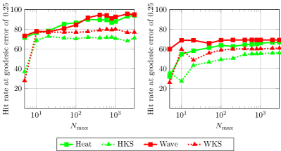
Figure 19: Results on the dataset wolf (left) and baby (right). Comparison of the geodesic error at $0.25$ between the optimised MCR technique and the kernel-based methods for different number of modes $N_{\max}\in[5,3000]$. The eigenvalues and eigenvectors for MCR and the kernel-based methods are computed by solving the symmetric and the generalised eigenvalue problem, respectively.

The results for both datasets, shown in Figure 19, clearly demonstrate a higher matching performance by using the optimised MCR technique. In almost all cases, the MCR signatures outperform their competitive methods HKS and WKS.

An interesting aspect is that the MCR heat signature yields slightly better results as WKS. Moreover, the depicted curves in Figure 19 show a saturation behaviour with respect to the number of used modes. Specifically, that means that the correspondence quality can no longer be significantly improved after a certain number of used modes.

Evaluation on TOSCA Dataset

First, let us also discuss here the number of the ordered modes for the mentioned methods. In many publications on the kernel-based methods this number is set manually to a fixed value (e.g. $N_{\max}=300$ is often used). Because of its impact on computational efficacy, we were motivated to consider here the examined measurements and the amount of used eigenvalues for the TOSCA dataset, see the results illustrated in Figure 20.

Over the whole dataset, we obtain qualitatively identical results as for the examples wolf and baby. The proposed MCR technique outperforms the kernel-based methods in terms of the geodesic error. For both PDEs, the optimised MCR method provides around 5-10% higher correspondence quality than the corresponding kernel-based approach. Again, in general the MCR heat signature slightly exceeds the performance of WKS. Additionally, the experiment indicates that for all methods a saturation behaviour is achieved at a small spectrum of $N\approx 100$ modes.

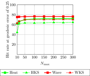
Figure 20: Results on the TOSCA dataset. Comparison of the geodesic error at $0.25$ between the optimised MCR technique and the kernel-based methods for a varying number of modes $N_{\max}$. The eigenvalues and eigenvectors for MCR and the kernel-based methods are computed by solving the symmetric and the generalised eigenvalue problem, respectively.

10.2 Soft Correspondence

For two discrete shapes $\mathcal{M}_{d}$ and $\mathcal{\widetilde{M}}_{d}$ with underlying point clouds $P=\{x_{1},\ldots,x_{N}\}$ and $\widetilde{P}=\{\widetilde{x}_{1},\ldots,\widetilde{x}_{\widetilde{N}}\}$, the matrix representation of the correspondence map $S_{\{0,1\}}\mathrel{\mathop{\mathchar 58\relax}}\widetilde{P}\times P\rightarrow\{0,1\}$ can be encoded by

$${S_{\{0,1\}}}_{ji}=\begin{cases}1,&{\mbox{if }}d_{f}(x_{i},\widetilde{x}_{j})\leq d_{f}(x_{i},\widetilde{x}_{k}),\quad k=1,\ldots,\widetilde{N}\\ 0,&\text{else}\end{cases}$$ (99)

where $S_{\{0,1\}}$ is a $(\widetilde{N}\times N)$ binary assignment matrix. For finding a single corresponding counterpart e.g. of $x_{i}\in P$ on $\mathcal{\widetilde{M}}_{d}$, we construct a vector-valued indicator function $h\mathrel{\mathop{\mathchar 58\relax}}P\rightarrow\{0,1\}$ with

$$\mathbf{h_{i}}(x_{k})={\begin{cases}1,&{\mbox{if }}i=k\\ 0,&{\mbox{else }}\end{cases}}$$ (100)

By performing matrix-vector multiplication $\mathbf{\widetilde{h}_{j}}={S_{\{0,1\}}}\mathbf{h_{i}}$, we obtain the indicator vector $\mathbf{\widetilde{h}_{j}}$ for the case the tuple $(x_{i},\widetilde{x}_{j})\in P\times\widetilde{P}$ is a corresponding pair.

However, due to strong elastic deformations, noisy shapes or intrinsic symmetries (i.e. inherent ambiguities) the construction (99) may generate misleading matchings. Therefore, the correspondence map $S_{\{0,1\}}$ is in practice neither injective nor surjective, even in the case $N=\widetilde{N}$.

By allowing values between 0 and 1, the correspondence map can be cast as a soft correspondence map $S_{[0,1]}\mathrel{\mathop{\mathchar 58\relax}}\widetilde{P}\times P\rightarrow[0,1]$, as used for example in Eisenberger2018 , which can be interpreted as a correspondence probability by using normalisation

$$\sum\limits_{i=1}^{N}{S_{[0,1]}}_{ji}=1,\quad j=1,\ldots,\widetilde{N}$$ (101)

For a certain point $x_{i}\in P$ on the reference shape the map encodes the transition probabilities to the points on $\widetilde{P}$ based on the feature distances, whereby high probabilities correspond to low feature distances and vice versa. The arising soft correspondence map allows us to express the probability transition of all points from a reference shape onto a target shape.

Let us briefly sketch an example for the usefulness of the approach. For this we make use of Figure 21 where we consider in particular the tail of the wolf. Similar to the pointwise case, we construct a discrete indicator function $\mathbf{h}$ with

$$\mathbf{h}(x_{i})={\begin{cases}1,&{\mbox{if }}x_{i}\in\text{Tail}\subset\mathcal{M}\\ 0,&{\mbox{else }}\end{cases}}$$ (102)

By performing $\mathbf{\widetilde{h}}=S_{[0,1]}\mathbf{h}$, the entries of $\mathbf{\widetilde{h}}$ contain the probability of the matched indicator function on the transformed shape.

Figure 21: Idea of mapping indicator functions: An indicator function (visualised by a colour map on the shape) $\mathbf{h}\in\mathcal{M}$ is defined such that it is one at the tail of the dog and zero else. Using the soft correspondence matrix, we define the probability of the matched indicator function $\mathbf{\widetilde{h}}\in\widetilde{\mathcal{M}}$ by performing $\mathbf{\widetilde{h}}=S_{[0,1]}\mathbf{h}$. For demonstration the optimised MCR heat method with $300$ modes was used. The probability of matching the indicator function on the tail of the transformed wolf is very high, while the colour encodes the probability ranging from white (almost zero probability) to black (probability of $10\%$ and higher). Since the ground truth is the identical labeling $(i,i)$, the soft correspondence matrix has a diagonal dominant structure.

Using soft correspondence maps in combination with the MCR technique may yield beneficial results when addressing problems like correspondence of shape segments or detection of intrinsically similar regions. The intuition behind this is that intrinsic feature descriptors have almost identical, low feature distances for whole regions where the intrinsic geometry is similar, and that such region-based information could favourably be described by low-frequency modes as used within MCR, whereas small details are described by high-frequency modes; see Figure 22 for an example.

Figure 22: Mapping of the indicator function defined on a certain region of the wolf shape (the front paw) to a transformed version of it. The colour encodes the probability of the matching, being black for a high probability and white for almost zero probability. The optimised MCR heat approach leads in this example to a better interpretation compared to the HKS, detecting similar regions of the shape reliably.

10.3 Sparsity of the Soft Correspondence Map

The soft correspondence map $S_{[0,1]}$ is a dense $(\widetilde{N}\times N)$-matrix, being increasingly cumbersome for large $\widetilde{N}$ and $N$. Especially for large shapes, the computation, storage and manipulation of $S_{[0,1]}$ might be computationally expensive. Therefore, it would be desirable to reduce the information contained in the dense matrix $S_{[0,1]}$, ideally computing from it the binary assignment matrix $S_{\{0,1\}}$ , however this task is in practice not trivial.

In the following, we demonstrate experimentally that it is possible to give $S_{[0,1]}$ a sparse structure while keeping its useful meaning for pointwise shape correspondence. The sparse structure appears to be a reasonable and computationally efficient compromise between the dense soft correspondence matrix and the ideal binary assignment matrix.

To increase sparsity we set iteratively small entries of $S_{[0,1]}$ (carrying a low probability) in ascending order w.r.t. the size of entries to zero. We assume in this context that the feature descriptor based on MCR delivers correct corresponding pairs for low feature distances (high probability entries of $S_{[0,1]}$) only.

Let us note that in each sparsification step one could normalise again the resulting matrix $S_{[0,1]}$ (which we do not give a different notion here as during sparsification it keeps its role as a soft correspondence matrix) so that one could again interprete it as probability transition matrix.

Evaluation Measure

In order to measure sparsity of the soft correspondence matrix, we define the density of $S_{[0,1]}$ by taking the ratio of the numbers of non-zero elements to the total number of elements (thus e.g. relative density of 100% means we have a full matrix). When using the ground truth in our experiments, we introduce the soft hit rate by evaluating if non-zero elements are transition probabilities leading to correct correspondences. It is obvious that the soft hit rate is correlated to the density of $S_{[0,1]}$, since the more non-zero elements are set to zero the more correct correspondences might accidentally be removed by the sparsification routine.

During sparsification, we seek a threshold density related to the individual example, such that the resulting matrices $S_{[0,1]}$ still contain the complete pointwise information of the underlying, ideal binary assignment matrix $S_{\{0,1\}}$. Therefore, we define the minimum density by taking the sparsest computed version of $S_{[0,1]}$ such that the soft hit rate still yields $100\%$ correct correspondences.

Evaluation on Wolf and Baby Datasets

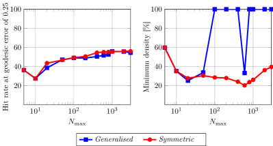
Figure 23: Results on the dataset baby by applying the heat kernel signature for a varying number of modes $N_{\max}\in[5,3000]$. Comparison of the geodesic error at $0.25$ (left) and the minimum density (right) between the construction of eigenvalues and eigenvectors by solving the generalised and the symmetric eigenvalue problem. Using the similarity transformation dramatically improves the sparsity of $S_{[0,1]}$.

Before we go into a more detailed evaluation on the sparsity of $S_{[0,1]}$, we revise the issue of the eigenvalue computation for the kernel-based methods. As demonstrated by the example of the baby dataset, cf. Figure 23, the way of construction of eigenvalues and eigenvectors affects the matching results. Even if the geodesic error accuracy remains almost identical, the modes computed by solving the generalised eigenvalue problem lead to a poor minimum density performance. For example, using $N_{\max}=100$ modes results to a minimum density of 100%. Therefore, HKS has to keep 100% of all correspondence probabilities in the underlying soft correspondence map $S_{[0,1]}$ for enabling to extract still a perfect matching of 100%, so that $S_{[0,1]}$ corresponds to a full (dense) matrix. Therefore, we employ the similarity transform also for the kernel-based methods for a more fair comparison with the MCR signatures.

We now compare the optimised MCR technique and the kernel-based methods for 100 eigenvalues using the dataset wolf and baby, respectively. The evaluation of the minimum density highlights the generally better correspondence capability of the MCR method, as shown in Figure 24 or Table 1. For the wolf and baby dataset the MCR wave and the MCR heat method with 4.86% and 18.85% (retained correspondence probabilities for enabling a perfect matching of 100%), respectively, outperform all other methods.

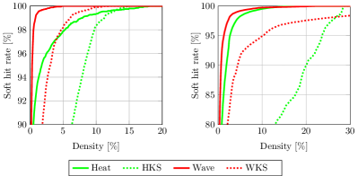
Figure 24: Results on the dataset wolf (left) and baby (right). Comparison of the relation in terms of soft hit rate and the density of $S_{[0,1]}$ between the optimised MCR technique and the kernel-based methods for $N_{\max}=100$ modes. The underlying eigenvalues and eigenvectors are computed by solving the symmetric eigenvalue problem. We observe that the MCR methods require a much lower number of entries in the soft corresponcdence matrix to capture correspondences.

Table 1: Results on the dataset wolf and baby by using the optimised MCR technique and the kernel-based methods for $N_{\max}=100$ modes. Comparison of the minimum density of $S_{[0,1]}$ for enabling to extract still a perfect matching of 100%. The corresponding curves are shown in Figure 24.

	Wolf	Baby
MCR heat	18.08%	18.85%
HKS	15.01%	28.54%
MCR wave	4.86%	22.63%
WKS	12.21%	62.3%

Evaluation on TOSCA Dataset

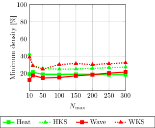
Figure 25: Results on the entire TOSCA dataset. Comparison of the minimum density between the optimised MCR technique and the kernel-based methods for a varying number of modes $N_{\max}$. The underlying eigenvalues and eigenvectors are computed by solving the beneficial symmetric eigenvalue problem. One clearly observes that the MCR methods rely on a much lower number of entries in the sparsified soft maps. Since we average here over the whole TOSCA dataset, this experiment demosntrates the robustness of the MCR approach in this respect.

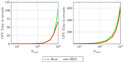
Figure 26: Results on the datasets wolf (left) and baby (right) by using the geometric heat equation. Comparison of the required computational time between the optimised MCR technique and the kernel-based methods for a varying number of modes $N_{\max}\in[5,1000]$. The underlying eigenvalues and eigenvectors are computed by solving the symmetric eigenvalue problem. The CPU time of the kernel-based methods is slightly faster in particular for $N_{\max}>100$ modes, however the MCR technique is clearly competitive. Using the geometric wave equation generates the same costs.

Also for the whole
TOSCA dataset, the MCR technique clearly outperforms the kernel-based methods in terms of the minimum density as shown in Figure 25. In general, the performance of the MCR wave method is the best one among all tested methods, however from $N_{\max}\approx 200$ modes on the MCR heat method gains in relevance. The most inferior results are achieved by using WKS, which generates for all used modes $N_{\max}\in[10,300]$ at least 10% worse density.

As in the previous examination in Section 10.1, the experiment shows that a small spectrum of eigenvalues ($N\approx 100$) works well for MCR as well as for the kernel-based methods. In this regime, the methods MCR wave, MCR heat, HKS and WKS result in required minimum density rates of 15.29%, 18.63%, 24.98% and 30.39%, respectively. The latter observation obviously demonstrates the benefits of using the MCR technique.

In the total, by using a small spectrum the computational effort may be reduced significantly without losing performance, which is especially important in the case of highly resolved meshes.

In a final experiment, we investigate the required computational time of the applied methods based on the wolf and baby dataset. As shown in Figure 26, both techniques achieve almost equally fast computational times.

11 Summary and Conclusion

We have extended the numerical framework that has been presented in earlier literature, and in our opinion we have tweaked with this paper the MOR approach very close to its limit concerning its use in shape correspondence construction. For achieving this we combined many numerical techniques with benefit that lead to an algorithm that is finally easy to implement.

Let us stress that our basic approach is nearly free of parameters, one can even conclude for the remaining few parameters like e.g. the number of eigenvalues that we have shown experimentally how to choose them in applications, so that in practice our approach can be considered as parameter-free, which is of high practical value.

We think that the use of the MCR technique for particular tasks in shape analysis, like e.g. symmetry or similarity detection, could be a promising subject of future research. Furthermore, the use of soft correspondences as studied here appears to be promising. As we pointed out and studied here for the first time in relation to our MOR approach to which it seems to fit quite well, it enables very high matching results and just needs sparse information for this in the soft correspondence matrix. It is not trivial and beyond the scope of this work to develop a method that could make full use of the soft correspondence information, which may result in a quite powerful approach.

Let us also note that as part of the functional maps pipeline mentioned in related work, feature descriptors are used to compute a coarse correspondence between points. Providing accurate initial correspondences based on feature descriptors will improve performance and computational time of dense shape correspondence algorithms relying on functional maps, as reported in MORCC . We conjecture that our method may also be useful in this context and we plan to investigate this in future research.

References

- (1) Antoulas, A.C.: Approximation of Large-Scale Dynamical Systems. Society for Industrial and Applied Mathematics, Philadelphia, PA, USA (2005)
- (2) Antoulas, A.C., Ionutiu, R., Martins, N., ter Maten, E.J.W., Mohaghegh, K., Pulch, R., Rommes, J., Saadvandi, M., Striebel, M.: Model Order Reduction: Methods, Concepts and Properties, pp. 159–265. Springer (2015)
- (3) Aubry, M., Schlickewei, U., Cremers, D.: The wave kernel signature: a quantum mechanical approach to shape analysis. In: Proceedings of the IEEE International Conference on Computer Vision, pp. 1626–1633 (2011)
- (4) Bähr, M., Breuß, M., Quéau, Y., Boroujerdi, A.S., Durou, J.D.: Fast and accurate surface normal integration on non-rectangular domains. Computational Visual Media 3(2), 107–129 (2017)
- (5) Bähr, M., Dachsel, R., Breuß, M.: Fast solvers for solving shape matching by time integration. In: M. Welk, M. Urschler, P.M. Roth (eds.) Proceedings of OAGM Workshop, pp. 65–72 (2018)
- (6) Baur, U., Benner, P., Feng, L.: Model order reduction for linear and nonlinear systems: A system-theoretic perspective. Archives of Computational Methods in Engineering 21, 331–358 (2014)
- (7) Belongie, S., Malik, J., Puzicha, J.: Shape context: A new descriptor for shape matching and object recognition. In: Advances in Neural Information Processing Systems, pp. 831–837 (2000)
- (8) Benzi, M.: Preconditioning techniques for large linear systems: A survey. Journal of Computational Physics 182(2), 418–477 (2002)
- (9) Boscaini, D., Masci, J., Melzi, S., Bronstein, M.M., Castellani, U., Vandergheynst, P.: Learning class-specific descriptors for deformable shapes using localized spectral convolutional networks. Computer Graphics Forum 35(5), 13–23 (2015)
- (10) Bronstein, A.M., Bronstein, M.M., Kimmel, R.: Numerical Geometry of Non-Rigid Shapes, 1st edn. Springer (2009)
- (11) Bronstein, M.A., Bronstein, M.M.: Shape recognition with spectral distances. Transactions on Pattern Analysis and Machine Intelligence 33(5), 1065–1071 (2011)
- (12) Bronstein, M.M., Kokkinos, I.: Scale-invariant heat kernel signatures for non-rigid shape recognition. In: Proceedings of the IEEE Computer Society Conference on Computer Vision and Pattern Recognition, pp. 1704–1711 (2010)
- (13) Carrière, M., Oudot, S., Ovsjanikov, M.: Stable topological signatures for points on 3d shapes. Computer Graphics Forum 34(5), 1–12 (2015)
- (14) Coifman, R.R., Lafon, S.: Diffusion maps. Applied and Computational Harmonic Analysis 21(1), 5–30 (2006)
- (15) Corman, R.R., Ovsjanikov, M., Chambolle, A.: Supervised descriptor learning for non-rigid shape matching. In: Computer Vision – ECCV 2014, vol. 8928, pp. 283–298 (2014)
- (16) Dachsel, R., Breuß, M., Hoeltgen, L.: The classic wave equation can do shape correspondence. In: M. Felsberg, A. Heyden, N. Krüger (eds.) Computer Analysis of Images and Patterns, vol. 10424, pp. 264–275 (2017)
- (17) Dachsel, R., Breuß, M., Hoeltgen, L.: Shape matching by time integration of partial differential equations. In: F. Lauze, Y. Dong, A. Dahl (eds.) Scale Space and Variational Methods in Computer Vision, vol. 10302, pp. 669–680 (2017)
- (18) Dachsel, R., Breuß, M., Hoeltgen, L.: A study of spectral expansion for shape correspondence. In: M. Welk, M. Urschler, P.M. Roth (eds.) Proceedings of the OAGM, pp. 73–79 (2018)
- (19) Davis, T.A.: Algorithm 930: Factorize: an object-oriented linear system solver for matlab. ACM Transactions on Mathematical Software 39(4), 1–18 (2013)
- (20) Do Carmo, M.P.: Differential geometry of curves and surfaces: revised and updated second edition. Dover Publications (2016)
- (21) Eisenberger, M., Lähner, Z., Cremers, D.: Divergence-free shape correspondence by deformation. Computer Graphics Forum 38, 1–12 (2019)
- (22) Eynard, D., Rodolà, E., Glashoff, K., Bronstein, M.M.: Coupled functional maps. In: 2016 Fourth International Conference on 3D Vision (3DV), pp. 399–407 (2016)
- (23) Gal, R., Shamir, A., Cohen-Or, D.: Pose-oblivious shape signature. Transactions on Visualization and Computer Graphics 13, 261–271 (2007)
- (24) Hafner, D., Ochs, P., Weickert, J., Reißel, M., Grewenig, S.: Fsi schemes: Fast semi-iterative solvers for pdes and optimisation methods. In: B. Rosenhahn, B. Andres (eds.) Pattern Recognition, vol. 9796, pp. 91–102 (2016)
- (25) Halimi, O., Litany, O., Rodolà, E., Bronstein, A., Kimmel, R.: Unsupervised learning of dense shape correspondence. In: Proceedings of the IEEE Computer Society Conference on Computer Vision and Pattern Recognition (2019)
- (26) He, X., Kong, Q., Xiao, Z.: Fast simulation methods for dynamic heat transfer through building envelope based on model-order-reduction. Procedia Engineering 121, 1764–1771 (2015)
- (27) Hestenes, M.R., Stiefel, E.: Methods of conjugate gradients for solving linear systems. Journal of research of the National Bureau of Standards 6(49), 46–70 (1952)
- (28) Ion, A., Artner, M.A., Peyr, G., Kropatsch, G.W., Cohen, D.L.: Matching 2d and 3d articulated shapes using the eccentricity transform. Computer Vision and Image Understanding 115(6), 817–834 (2011)
- (29) Johnson, A., Herbert, M.: Using spin images for efficient object recognition in cluttered 3d scenes. IEEE Transactions on Pattern Analysis and Machine Intelligence 21(5), 433–449 (1999)
- (30) van Kaick, O., Zhang, H., Hamarneh, G., Cohen-Or, D.: A survey on shape correspondence. Computer Graphics Forum 30(6), 1681–1707 (2011)
- (31) Kim, V.G., Lipman, Y., Funkhouser, T.: Blended intrinsic maps. ACM Transactions on Graphics 30(4) (2011)
- (32) Kimmel, R., Sethian, A.: Computing geodesic paths on manifolds. Proceedings of the National Academy of Sciences 95(15), 8431–8435 (1998)
- (33) Lévy, B.: Laplace-beltrami eigenfunctions towards an algorithm that ‘understands’ geometry. In: Proceedings of the IEEE International Conference on Shape Modeling and Applications (2006)
- (34) Litany, O., Remez, T., Rodolà, E., Bronstein, A., Bronstein, M.M.: Deep functional maps: Structured prediction for dense shape correspondence. In: Proceedings of the IEEE International Conference on Computer Vision, pp. 5660–5668 (2017)
- (35) Litman, R., Bronstein, M.A.: Learning spectral descriptors for deformable shape correspondence. Transactions on Pattern Analysis and Machine Intelligence 36(1), 170–180 (2014)
- (36) Litman, R., Bronstein, M.A., Bronstein, M.M., Castellani, U.: Supervised learning of bag-of-features shape descriptors using sparse coding. Computer Graphics Forum 33(5), 127–136 (2014)
- (37) Lowe, D.G.: Distinctive image features from scale-invariant keypoints. International Journal of Computer Vision 60(2), 91–110 (2004)
- (38) Manay, S., Hong, B.W., Yezzi, A.J., Soatto, S.: Integral invariant signatures. In: Computer Vision – ECCV 2004, pp. 87–99 (2004)
- (39) Melzi, S., Ovsjanikov, M., Roffo, G., Cristani, M., Castellani, U.: Discrete time evolution process descriptor for shape analysis and matching. ACM Transactions on Graphics 37 (2018)
- (40) Melzi, S., Ren, J., Rodolà, E., Sharma, A., Wonka, P., Ovsjanikov, M.: Zoomout: Spectral upsampling for efficient shape correspondence. In: Proceedings of the ACM SIGGRAPH Asia (2019)
- (41) Melzi, S., Rodolà, E., Castellani, U., Bronstein, M.M.: Proceedings of the international conference on 3d vision. In: Shape analysis with anisotropic windowed Fourier transform, pp. 470–478 (2016)
- (42) Meurant, G.: Computer Solution of Large Linear Systems, 1st edn. Elsevier Science (1999)
- (43) Meyer, M., Desbrun, M., Schröder, P., Barr, A.H.: Discrete differential-geometry operators for triangulated 2-manifolds. In: H.C. Hege, K. Polthier (eds.) In Visualization and Mathematics III, pp. 35–57 (2002)
- (44) Ojo, S.O., Grivet-Talocia, S., Paggi, M.: Model order reduction applied to heat conduction in photovoltaic modules. Composite Structures 119, 477–486 (2015)
- (45) Osada, R., Funkhouser, T., Chazelle, B., Dobkin, D.: Shape distributions. ACM Transaction on Graphics 21, 807–832 (2002)
- (46) Ovsjanikov, M., Ben-Chen, M., Solomon, J., Butche, A., Guibas, L.: Functional maps: a flexible representation of maps between shapes. ACM Transactions on Graphics 31, 30:1–30:11 (2012)
- (47) Parlett, B.N.: The Symmetric Eigenvalue Problem. Prentice-Hall (1998)
- (48) Pottmann, H., Wallner, H., Huang, Q.X., Yang, Y.L.: Integral invariants for robust geometry processing. Computer Aided Geometric Design 26(1), 37–60 (2009)
- (49) Reuter, M., Biasotti, S., Giorgi, D., Patanè, G., Spagnuolo, M.: Discrete Laplace–Beltrami operators for shape analysis and segmentation. Computers & Graphics 33(3), 381–390 (2009)
- (50) Rodolà, E., Bulo, S.R., Windheuser, T., Vestner, M., Cremers, D.: Dense non-rigid shape correspondence using random forests. In: Proceedings of the IEEE Computer Society Conference on Computer Vision and Pattern Recognition, pp. 4177–4184 (2014)
- (51) Rodolà, E., Cosmo, L., Bronstein, M.M., Torsello, A., Cremers, D.: Partial functional correspondence. Computer Graphics Forum 36(1), 222–236 (2017)
- (52) Rodolà, E., Lähner, Z., Bronstein, M.A., Bronstein, M.M., Solomon, J.: Functional maps representation on product manifolds. Computer Graphics Forum 38(1), 678–689 (2019)
- (53) Rustamov, R.M.: Laplace-beltrami eigenfunctions for deformation invariant shape representation. In: A. Belyaev, M. Garland (eds.) Proceedings of the Eurographics symposium on geometry processing, pp. 225–233 (2007)
- (54) Saad, Y.: Iterative Methods For Sparse Linear Systems, 2nd edn. Society for Industrial and Applied Mathematics (2003)
- (55) Salimbahrami, B., Lohmann, B.: Krylov subspace methods in linear model order reduction: Introduction and invariance properties. Tech. rep., Institute of Automation, University of Bremen (2002)
- (56) Sauvigny, F.: Partial Differential Equations 2 – Functional Analytic Methods. Springer (2012)
- (57) Selga, R.C., Lohmann, B., Eid, R.: Stability preservation in projection-based model order reduction of large scale systems. European Journal of Control 18, 122–132 (2012)
- (58) Smith, G.D.: Numerical Solution of Partial Differential Equations: Finite Difference Methods. Clarendon Press, Oxford Applied Mathematics and Computing Science Series (1985)
- (59) Solomon, J., Nguyen, A., Butscher, A., Ben-Chen, M., Guibas, L.: Soft maps between surfaces. Computer Graphics Forum 31(5), 1617–1626 (2012)
- (60) Sun, J., Ovsjanikov, M., Guibas, L.: A concise and provably informative multi-scale signature based on heat diffusion. Computer Graphics Forum 28(5), 1383–1392 (2009)
- (61) Surazhsky, V., Surazhsky, T., Kirsanov, D., Gortler, S.J.: Fast exact and approximate geodesics on meshes. ACM Transaction on Graphics 24, 553–560 (2005)
- (62) Tombari, F., Salti, S., Stefano, D.L.: Unique signatures ofhistograms for local surface description. In: Proceedings of the IEEE International Conference on Computer Vision, pp. 356–369 (2010)
- (63) Varadhan, S.R.S.: On the behaviour of the fundamental solution of the heat equation with variable coefficients. Communications on Pure and Applied Mathematics 20(2), 431–455 (1967)
- (64) Vestner, M., Litman, R., Rodolà, E., Bronstein, m.A., Cremers, D.: Product manifold filter: Non-rigid shape correspondence via kernel density estimation in the product space. In: Proceedings of the IEEE Computer Society Conference on Computer Vision and Pattern Recognition (2017)
- (65) Yang, Y.L., Lai, Y.K., Hu, S.M., Pottmann, H.: Robust principal curvatures on multiple scales. In: Proceedings of the fourth Eurographics symposium on geometry processing, pp. 223–226 (2006)
- (66) Zaharescu, A., Boyer, E., Horaud, R.: Keypoints and local descriptors of scalar functions on 2d manifolds. International Journal of Computer Vision 100(1), 78–98 (2012)
- (67) Zhang, H., van Kaick, O., Dyer, R.: Spectral mesh processing. Computer Graphics Forum 29(6), 1865–1894 (2010)
- (68) Šindler, J., Suleng, A., Olsen, T.J., Bárta, P.: Krylov model order reduction of a thermal subsea model. International Journal of Mechanical, Aerospace, Industrial, Mechatronic and Manufacturing Engineering 7(5), 842–849 (2013)