Influence of nanoparticle surface and shape on the dipole magnetic absorption of ultrashort laser pulses

Abstract

The theory on the magnetic field energy absorption by metal nanoparticles of a nonspherical shape irradiated with ultrashort laser pulses of different duration is developed. The effect of both the particle surface and the particle shape on the absorbed energy is studied. For the particles having an oblate or prolate spheroidal shape, the dependence of this energy on the orientation of the magnetic field upon a particle, the degree of its deviation from a spherical shape, a pulse duration, and the carrier frequency of the laser ray are found. A significant increase in the absorption is established when an electron mean free path coincides with the size of the particle. The Drude and kinetic approaches are used and the results are compared with each other.

Key words: metal nanoparticles, dipole magnetic absorption, ultrashort laser pulses, nonspherical particles

PACS: 78.67.-n, 65.80.-g, 73.23.-b, 68.49.Jk, 52.25.Os

Abstract

Розвинуто теорiю поглинання енергiї магнiтного поля металевими наночастинками несферичної форми, опромiнених ультракороткими лазерними iмпульсами рiзної тривалостi. Вивчається вплив як поверхнi частинки, так i її форми на величину поглинутої енергiї. Для частинок сплюснутої чи витягнутої форми знайдена залежнiсть цiєї енергiї вiд орiєнтацiї магнiтного поля вiдносно частинки, ступеня вiдхилення її форми вiд сферичної, тривалостi iмпульсу та вiд несучої частоти лазерного променя. Встановлений значний рiст у поглинаннi, коли середня довжина вiльного пробiгу електрона збiгається з розмiрами частинки. Для обчислень використовувались пiдходи Друде та кiнетичний i їх результати порiвнювались.

Ключовi слова: металевi наночастинки, дипольне магнiтне поглинання, ультракороткi лазернi iмпульси, несферичнi частинки

1 Introduction

With the help of pulses of short duration, it is possible to study the dynamics of rapid processes occurring in atoms, molecules and solids. Pico- and femtosecond resolution allows one to study oscillatory and rotational intra-molecular movements, carrier dynamics in semiconductor nanostructures, phase transitions in solids, formation and breakdown of chemical bonds, etc. [1, 2].

In recent years, there has been a continuous experimental attention paid to the study of ultrashort dynamics of electrons in metallic nanoparticles (MNs). The increase of local magnetic fields close to MNs makes them useful as markers in biological systems [3, 4], in biosensing for magnetic particle detection techniques [5], as well as in magnetic diagnostic systems [6]. In general, nanostructures are widely used in modern high-speed electronics and optoelectronics.

Modern optical devices provide an opportunity to record the optical response of a single nanoparticle and thus allow one to study the properties of separate nanobjects [7]. This opens up new direct possibilities for sensing multi-electronic dynamics in limited systems.

Theoretical treatment of the magnetic dipole absorption was proposed by Wilkinson and coauthors in [8]. The enhanced absorption of a surface plasma wave by MNs in the presence of an external magnetic field was studied recently in [9]. The possibility for nanoparticles to produce a strong magnetic dipole absorption at optical frequencies has also been noticed by authors of [10]. The major role of magnetic field losses in microwave heating of metal was demonstrated in [11].

Interesting results on the aforementioned problems were recently obtained in [12, 13, 14, 15, 16]. Particularly, in [13, 12], it was demonstrated that the magnetic dipole resonances and the magnetic response can be detected even in the dielectric nanospheres.

As is known, the absorption by MNs in the field of a monochromatic electromagnetic (EM) wave, whose length is much larger than the size of the particle, is due to the contribution both from the electrical component of the EM wave (electrical absorption) and the magnetic component (magnetic absorption) [17, 18].

In previous studies [19, 20, 21, 22], we have shown that depending on the size of the particle, as well as on the frequency and polarization of the wave, the magnetic absorption can be either larger or smaller than the electric one.

The situation may change with the use of ultrashort pulses. Firstly, the ultrashort pulse contains almost all the harmonics, including those that coincide with plasmon resonances. It allows all the resonances inherent in the system to manifest themselves, and to study the system response in general. Secondly, the frequency distribution over the ultrashort pulse spectrum is highly heterogeneous (Gaussian). The above factors may change the relation between the electrical and magnetic absorption contribution.

We studied the features of electrical absorption of ultrashort pulses in [21]. In this paper, we focus on the research of the absorption characteristics due to the effect of the magnetic component of the ultrashort EM pulse. This problem remains little studied, especially for the MS of a non-spherical form with dimensions both smaller and larger than the electron mean free path. The main goal of this study is to investigate how the surface and shape of the particle can manifest themselves in the dipole magnetic absorption of ultrashort laser pulses.

The work is structured as follows. The second section describes the model and the main principles of the problem. The third section is devoted to the study of magnetic absorption with Drude and kinetic approaches. The fourth section discusses the results and the fifth section presents the main results and conclusions.

2 Model and main principles

Let the laser pulse fall on the MN, the electric field of which we take in the form [21]

$${\rm{\bf E}}({\rm{\bf r}},t)={\rm{\bf E}}_{0}\mathrm{e}^{-\Gamma^{2}\left(t-\frac{{\rm\bf k}_{\text{c}}{\rm\bf r}}{\omega_{\text{c}}}\right)^{2}}\cos{\left[{\omega_{\text{c}}\left({t-{\frac{{{\rm{\bf k}}_{\text{c}}{\rm{\bf r}}}}{{\omega_{\text{c}}}}}}\right)}\right]},$$ (2.1)

where $\Gamma$ is the value reversed to the duration of the laser pulse, $\omega_{\text{c}}$ is a carrier frequency of the EM wave, $|{\rm{\bf k}}_{\text{c}}|\;=\omega_{\text{c}}/c$, and ${\rm{\bf E}}_{0}$ has the sense of the maximum value of the electric field in the pulse. In addition to the electric field, the laser pulse field also has a magnetic component, which is connected with the electrical component by the corresponding Maxwell equation

$$\operatorname{rot}{{\bf E}}({\rm{\bf r}},t)=-{\frac{{1}}{{c}}}{\frac{{\partial}}{{\partial t}}}{\rm{\bf H}}({\rm{\bf r}},t).$$ (2.2)

By taking ${\rm{\bf E}}({\rm{\bf r}},t)$ in the form of equation (2.1), we establish with the help of equation (2.2), the value of the magnetic field. Most simply, this connection will be seen between the Fourier components of these quantities.

Making the Fourier transform in equation (2.2), and performing the integration over time in the limits $(-\infty,\infty)$, we find for the value of the magnetic field the form

$${\rm{\bf H}}({\rm{\bf r}},\omega)=\frac{\sqrt{\piup}}{2\Gamma}\left[\mathrm{e}^{-{\frac{(\omega-\omega_{\text{c}})^{2}}{4\Gamma^{2}}}}+\mathrm{e}^{-{\frac{(\omega+\omega_{\text{c}})^{2}}{4\Gamma^{2}}}}\right]\mathrm{e}^{\mathrm{i}{\rm\bf k}_{\text{c}}{\rm\bf r}\big{(}\frac{\omega}{\omega_{\text{c}}}\big{)}}\rm{\bf m}\times{\rm{\bf E}}_{0}\,,$$ (2.3)

where ${\rm\bf m}={\rm\bf k}_{\text{c}}/k_{\text{c}}$ is the unit vector directed along the direction of the EM wave propagation.

The magnetic field of the laser pulse generates the rotational electric field ${\rm{\bf E}}_{\text{rot}}({\rm{\bf r}},t)$ inside the MN. To find an expression for the energy absorbed by MN, it is necessary to know the internal field ${\rm{\bf E}}_{\text{rot}}({\rm\bf r},t)$. In order to determine it, we pay attention to the multiplier feature of the Fourier component in equation (2.3) related to the coordinate dependence. If the characteristic size of the nanoparticle $R$ is such that $k_{\text{c}}R\ll 1$, that is, the length of the carrier wave is much greater than the size of the MN, then the coordinate dependence of the Fourier-component ${\rm{\bf H}}({\rm{\bf r}},\omega)$ within the particle can be neglected. This means that it is possible to determine the Fourier component of the internal field inside the MN as a spatially homogeneous, ${\rm{\bf H}}({\rm{\bf r}},\omega)\to{\rm{\bf H}}(0,\omega)$.

For an asymmetric MN having, for example, an ellipsoid shape, this allows us to write a circular electric field

$$[{\rm{\bf E}}_{\text{rot}}({\rm{\bf r}},\omega)]_{x}\approx\mathrm{i}{\frac{\omega}{c}}\left[{\frac{H_{y}(0,\omega)}{c^{2}+a^{2}}}z-{\frac{{H_{x}(0,\omega)}}{a^{2}+b^{2}}}y\right]a^{2},$$ (2.4)

as in [21]. The rest of the components of the rotational field can be obtained from equation (2.4) by cyclic permutation of indices. In equation (2.4), parameters $a$, $b$, and $c$ are the ellipsoid half-axes in the directions $x$, $y$ and $z$, respectively. The linear dependence of the rotational field on the coordinates is easy to understand from equation (2.2), that defines this field. If we make the time Fourier transform of equation (2.2), then the right-hand side of this equation (as can be seen from equation (2.3) and the assumed inequality) can be considered as a constant not dependent on coordinates. This means that $\operatorname{rot}{\rm{\bf E}}_{\text{rot}}({\rm{\bf r}},\omega)=\text{const}$. However, such an equality is possible only in the single case when

$$[{\rm{\bf E}}_{\text{rot}}({\rm{\bf r}},\omega)]_{j}={\sum\limits_{k=1}^{3}{\alpha_{jk}(\omega)\,x_{k}}}\,,$$ (2.5)

that is, the rotational field is linearly dependent on the coordinates. Here, $\alpha$ is some matrix not dependent on ${\rm{\bf r}}$, the components of which we will further specify.

From equation (2.4) one can see that the homogeneous external magnetic field induces the coordinate-dependent rotational field inside the particle. The internal field ${\rm{\bf E}}_{\text{rot}}({\rm{\bf r}},t)$ generates the corresponding density of current ${\rm{\bf j}}_{\text{rot}}({\rm{\bf r}},t)$ in the MN. As a result, the particle absorbs the energy from the EM field of the incident laser wave.

3 Dipole magnetic absorption

When the MN is illuminated by the field of a monochromatic EM wave and the wave frequency is far from the plasmon resonance, the electrical or the magnetic absorption can dominate depending on the size of the MN [16, 20]. However, if the size of the spherical MN exceeds 50 Å, then the magnetic absorption prevails the electrical one for different polarizations of the incident light (starting at frequencies smaller than the refraction frequency of the electrons from the walls of the MN).

Relying on the Parseval correlation for the Fourier integral [23], the energy of the magnetic absorption can be represented as

$$w_{\text{m}}={\int\limits_{-\infty}^{\infty}W(t)\mathrm{d}t}=\frac{1}{2}\int\limits_{-\infty}^{\infty}{\frac{{\mathrm{d}\omega}}{2\piup}}\mathop{\symoperators Re}\nolimits\int\limits_{V}{\rm{\bf j}}_{\text{rot}}({\rm{\bf r}},\omega){\rm{\bf E}}_{\text{rot}}^{\ast}({\rm{\bf r}},\omega)\mathrm{d}{\rm{\bf r}},$$ (3.1)

where integration should be carried out over the entire volume of the particle, $W(t)$ is the absorbed power.

The quantity ${\rm{\bf E}}_{\text{rot}}({\rm{\bf r}},\omega)$ in accordance with equation (2.4) is already known. Thus, the task remains to find the Fourier component of the current density ${\rm{\bf j}}_{\text{rot}}({\rm{\bf r}},\omega)$. In the general case, the current at the point ${\rm{\bf r}}$ of a particle caused by the rotational field ${\rm{\bf E}}_{\text{rot}}({\rm{\bf r}},\omega)$ can be written as an integral over all electron velocities ${\bf v}$

$${\rm{\bf j}}({\rm{\bf r}},\omega)=2e\left({\frac{m}{2\piup\hbar}}\right)^{3}{\int_{-\infty}^{\infty}{{\rm{\bf v}}f_{1}({\rm{\bf r}},{\rm{\bf v}},\omega)}\mathrm{d}^{3}\upsilon},$$ (3.2)

where $\upsilon=|{\bf v}|$, $f_{1}({\rm{\bf r}},{\rm{\bf v}},\omega)$ is the Fourier component of a nonequilibrium distribution function, which is considered as an addition to the equilibrium Fermi distribution function $f_{0}({\cal E})$ dependent only on the electron kinetic energy ${\cal E}$. The function $f_{1}({\rm{\bf r}},{\rm{\bf v}},\omega)$ is sought as the solution of the corresponding linearized Boltzmann kinetic equation. As a rule, it is written as a time dependent function (see, for example, [21]). If we perform the Fourier transform of this equation and take into account the Fourier integral (2.3) for the field, and also

$$f_{1}({\rm{\bf r}},{\rm{\bf v}},\omega)={\int\limits_{-\infty}^{\infty}{f_{1}({\rm{\bf r}},{\rm{\bf v}},t)\,\mathrm{e}^{\mathrm{i}\omega t}}}\mathrm{d}t,$$ (3.3)

we consequently get for $f_{1}$ the following equation

$$(\nu-\mathrm{i}\omega)f_{1}({\rm{\bf r}},{\rm{\bf v}},\omega)+{\rm{\bf v}}{\frac{\partial f_{1}({\rm{\bf r}},{\rm{\bf v}},\omega)}{\partial{\rm{\bf r}}}}+e{\rm{\bf E}}_{\text{rot}}({\rm{\bf r}},\omega)\;{\frac{\partial f_{0}({\cal E})}{\partial{\rm{\bf p}}}}=0,$$ (3.4)

where $\nu$ is the frequency of bulk collisions of an electron, ${\rm{\bf p}}=m{\rm{\bf v}}$. The equation (3.4) should be supplemented by the corresponding boundary conditions. As such, we have chosen the conditions for a diffuse reflection of electrons from the internal walls of the particle

$$f_{1}({\rm{\bf r}},{\rm{\bf v}},\omega)|_{S}=0,\quad\quad\upsilon_{n}<0.$$ (3.5)

In equation (3.5), the value $\upsilon_{n}$ is the component of the velocity normal to the surface $S$. The reasoning for such boundary conditions can be found, in particular, in [24].

To solve equation (3.4) with the boundary conditions (3.5), it is convenient to pass to the deformed variables

$$x_{i}^{\prime}=Rx_{i}/\rho_{i}\,,\quad\upsilon_{j}^{\prime}=R\upsilon_{j}/\rho_{j}.$$ (3.6)

The primed $x_{i}^{\prime}$ and $\upsilon_{j}^{\prime}$ symbols indicate the compression-stretching coordinates and velocities, which permit to modify an ellipsoidal particle (with semiaxes $a,b,c$) into a spherical particle [with the radius $R=(abc)^{1/3}$], and $\rho_{x}=a$, $\rho_{y}=b$, $\rho_{z}=c$. Such modification changes only the shape of the particle leaving the volume unchanged. Then the solution of equation (3.4) will take the form

$$f_{1}({\rm{\bf r}}^{\prime},{\rm{\bf v}}^{\prime},\omega)=-\frac{e}{R^{2}}\frac{\partial f_{0}}{\partial{\cal E}}\sum\limits_{i,j=1}^{3}\alpha_{ij}(\omega)\;\upsilon^{\prime}_{j}\;\rho_{j}\rho_{i}\left[{x^{\prime}_{i}+\upsilon^{\prime}_{i}\frac{\partial}{\partial(\nu-\mathrm{i}\omega)}}\right]\frac{1-\mathrm{e}^{-(\nu-\mathrm{i}\omega)\,t^{\prime}({\rm{\bf r}}^{\prime},{\rm{\bf v}}^{\prime})}}{\nu-\mathrm{i}\omega}\,,$$ (3.7)

where

$$t^{\prime}({\rm{\bf r}}^{\prime},{\rm{\bf v}}^{\prime})={\frac{1}{\upsilon^{\prime 2}}}\big{[}{\rm{\bf r}}^{\prime}{\rm{\bf v}}^{\prime}+\sqrt{(R^{2}-r^{\prime 2})\upsilon^{\prime 2}+({\rm{\bf r}}^{\prime}{\rm{\bf v}}^{\prime})^{2}}\big{]}.$$ (3.8)

The diagonal components of the matrix $\alpha_{ij}$ are $\alpha_{jj}=0$, and the non-diagonal ones are expressed through the corresponding components of the magnetic field. For example,

$$\alpha_{xy}(\omega)=-\mathrm{i}{\frac{{\omega}}{c}}{\frac{a^{2}}{{a^{2}+b^{2}}}}H_{z}(0,\omega).$$ (3.9)

Two components of the matrix $\alpha_{ij}$ can be obtained by cyclic permutation of the indices in equation (3.9). The remaining three components can be found using skew-symmetry of $\alpha$, that is, taking into account the property: $\alpha_{xy}(\omega)=-\alpha_{yx}(\omega)$.

Thus, to find the energy of the magnetic absorption of laser pulses, it is necessary to perform the following steps: substitute the found function $f_{1}({\bf r},{\bf v},\omega)$ into equation (3.2) to obtain the Fourier component of the current density and then substitute both the current density and the rotational field given by equation (2.4) into equation (3.1).

The calculation of the absorption energy can be carried out avoiding the described procedure using the Drude approach in the study of the current.

3.1 Drude approach

Let the particle size be greater than the electron mean free path within it. Then, we can express the rotational current in terms of the rotational field as ${\rm{\bf j}}_{\text{rot}}(\omega)=\sigma_{\text{m}}(\omega)\;{\rm{\bf E}}_{\text{rot}}(\omega)$, and equation (3.1) can be rewritten in the form

$$w_{\text{m}}={\frac{1}{2}}{\sum\limits_{j=1}^{3}\mathop{\symoperators Re}\nolimits{{\int_{-\infty}^{\infty}{\sigma_{\text{m}}(\omega)\;{\frac{\mathrm{d}\omega}{2\piup}}\;{\int_{V}{|{\rm{\bf E}}_{\text{rot}}^{j}({\rm{\bf r}},\omega)|^{2}\mathrm{d}{\rm\bf r}}}}}}}.$$ (3.10)

Integration over the volume of the ellipsoid in equation (3.10) can be replaced by integration over the sphere of an equivalent volume.

We will restrict ourselves further to the consideration of metal nanoparticles with the spheroidal shape ($a=b\equiv\rho_{\bot}$, $c\equiv\rho_{\|})$. Using equations (2.4) and elementary integration over electron coordinates, the sum of integrals over a nanoparticle volume will be

$$\sum\limits_{j=1}^{3}\int_{V}{|{\rm{\bf E}}_{\text{rot}}^{j}({\rm{\bf r}},\omega)|}^{2}\mathrm{d}{\rm{\bf r}}=\frac{V}{5}\left(\frac{\omega\rho_{\bot}}{c}\right)^{2}\left[\frac{\rm{\bf H}_{\|}^{2}(0,\omega)}{2}+\xi\,{\rm{\bf H}}_{\bot}^{2}(0,\omega)\right].$$ (3.11)

Here,

$$\xi=\rho_{\|}^{2}/(\rho_{\|}^{2}+\rho_{\bot}^{2}),$$ (3.12)

${\rm{\bf H}}_{\|}(0,\omega)$ is the intensity of the magnetic field along the spheroid rotation axis, and ${\rm{\bf H}}_{\bot}(0,\omega)$ — across this axis. We note that the magnetic absorption significantly depends on the magnetic field polarization. Equation (3.11) can be generalized to the case of an arbitrary coordinate system if the components of the field are represented as:

$${\rm{\bf H}}_{\bot}^{2}={\rm{\bf H}}^{2}-{\rm{\bf H}}_{\|}^{2}\,,\qquad{\rm{\bf H}}_{\|}=({\rm{\bf H}}\cdot{\rm{\bf n}}){\rm{\bf n}}\,,$$ (3.13)

where ${\rm{\bf n}}$ is a unit vector directed along the spheroid axis of rotation. Then, with an account of equations (3.11)–(3.13), the expression (3.10) transforms into

$$w_{\text{m}}=\frac{V}{10}\left(\frac{\omega\rho_{\bot}}{c}\right)^{2}\xi\mathop{\symoperators Re}\nolimits\int_{-\infty}^{\infty}{\frac{\mathrm{d}\omega}{2\piup}}\sigma_{\text{m}}(\omega)\,\left\{{\rm{\bf H}}^{2}(0,\omega)-\frac{1}{2}\left({1-\frac{\rho_{\bot}^{2}}{\rho_{\|}^{2}}}\right)[{\rm{\bf H}}(0,\omega){\rm{\bf n}}]^{2}\right\}.$$ (3.14)

The field ${\rm{\bf H}}(0,\omega)$ in equation (3.14) is given by equation (2.3), and the dependence $\sigma_{\text{m}}(\omega)$ for the metal particle in the Drude approach is

$$\sigma_{\text{m}}(\omega)={\frac{1}{4\piup}}{\frac{\omega_{\text{pl}}^{2}}{\nu-\mathrm{i}\omega}}\,,$$ (3.15)

where $\omega^{2}_{\text{pl}}=4\piup ne^{2}/m$ is the frequency of plasma oscillations of electrons in a metal.

Next, we will perform calculations for specific polarizations of the magnetic wave relative to the MN orientation. Consider the following two cases:

(i) The magnetic field is directed across the spheroid axis. Then, the second term under the integral in equation (3.14) vanishes and after substituting equations (2.3) and (3.15) into equation (3.14), we obtain an expression for the absorbed energy

$$w_{\text{m}\bot}=\frac{V\xi}{160}\frac{\nu}{\Gamma^{2}}\left(\frac{\omega_{\text{pl}}\rho_{\bot}}{c}\right)^{2}|{\rm{\bf H}}_{0}|^{2}{\int\limits_{-\infty}^{\infty}{\frac{\mathrm{d}\omega}{2\piup}}{{\frac{{\omega^{2}f(\omega)}}{\nu^{2}+\omega^{2}}}}}\,,$$ (3.16)

with

$$f(\omega)=\left\{{\exp{\left[{-{\frac{{(\omega-\omega_{\text{c}})^{2}}}{4\Gamma^{2}}}}\right]}+\exp{\left[{-{\frac{{(\omega+\omega_{\text{c}})^{2}}}{4\Gamma^{2}}}}\right]}}\right\}^{2}.$$ (3.17)

The exact integration in equation (3.16) is not possible in an analytical form. However, taking into account that the frequency of electron bulk collisions $\nu\approx 10^{13}$ s^-1 is a small value comparing to the frequencies $\omega\approx\omega_{\text{c}}\sim 10^{15}$ s^-1 which provide the main contribution to the integral, one can neglect by $\nu$ in the integrand of equation (3.16). Then, we come to twice the integral $I_{\nu}={\int_{\nu}^{\infty}{f(\omega)}}\mathrm{d}\omega.$

This integral can be calculated analytically even within pointed limits. However, it is not difficult to make sure that the result of the integration is practically unchanged if the lower limit of integration in the integral $I_{\nu}$ is lowered to zero. This means that the integral $I={\int_{0}^{\nu}{f(\omega)}}\mathrm{d}\omega$ within the limits [0,$\nu$] is much smaller compared to $I_{\nu}$, and it can be omitted. Thus, for an integral within the limits $[0,\infty]$, we find:

$${\int\limits_{0}^{\infty}{\left\{{\exp{\left[{-{\frac{(\omega-\omega_{\text{c}})^{2}}{4\Gamma^{2}}}}\right]}+\exp{\left[{-{\frac{(\omega+\omega_{\text{c}})^{2}}{4\Gamma^{2}}}}\right]}}\right\}^{2}}}\mathrm{d}\omega=\sqrt{2\piup}\;\Gamma\left[{1+\exp{\left({-{\frac{{\omega_{\text{c}}^{2}}}{{2\Gamma^{2}}}}}\right)}}\right],$$ (3.18)

and as a result

$$w_{\text{m}\bot}=\frac{1}{80}{\frac{V\xi}{{\sqrt{2\piup}}}}{\frac{{\nu}}{{\Gamma}}}\left(\frac{\omega_{\text{pl}}\rho_{\bot}}{c}\right)^{2}\left({1+\mathrm{e}^{-{\frac{\omega_{\text{c}}^{2}}{2\Gamma^{2}}}}}\right)|{\rm{\bf H}}_{0}|^{2},$$ (3.19)

provided that $\omega\gg\nu$. If the ratio of $\omega_{\text{c}}/\Gamma>1$, then the second term in parentheses can be omitted, but if the ratio of $\omega_{\text{c}}/\Gamma\rightarrow 0$, then the result for $w_{\text{m}\bot}$ doubles.

(ii) Now, let us pass to the polarization of the EM wave, when the magnetic field is directed along the spheroid axis. Then, the scalar product in the second term under the integral in equation (3.14) is ${\rm{\bf H}}(0,\omega)\,{\rm{\bf n}}=|{\rm{\bf H}}(0,\omega)|$ and substituting equation (2.3) into equation (3.14), we find the expression

$$w_{\text{m}\|}=\frac{V}{80}\frac{\piup}{\Gamma^{2}}\frac{\rho_{\bot}^{2}}{c^{2}}|{\rm{\bf H}}_{0}|^{2}\mathop{\symoperators Re}\nolimits{\int\limits_{-\infty}^{\infty}\frac{\mathrm{d}\omega}{2\piup}\omega^{2}\sigma_{\text{m}}(\omega)f(\omega)}.$$ (3.20)

Using equation (3.15) and the result of the integration in equation (3.18), we arrive finally at the expression for the energy absorbed with this polarization

$$w_{\text{m}\|}={\frac{1}{160}}{\frac{V}{{\sqrt{2\piup}}}}{\frac{\nu}{\Gamma}}\left({{\frac{{\omega_{\text{pl}}\rho_{\bot}}}{c}}}\right)^{2}\left({1+\mathrm{e}^{-{\frac{\omega_{\text{c}}^{2}}{2\Gamma^{2}}}}}\right)|{\rm{\bf H}}_{0}|^{2},$$ (3.21)

provided that $\omega\gg\nu$. Obviously, for a spherical MN $\xi=1/2$ in equation (3.19) and it is necessary to replace $\rho_{\bot}$ by $R$ in equations (3.19) and (3.21).

If we assume that the monochromatic EM wave is falling on the nanoparticle, that is the wave is described by equation (2.1) with $\Gamma\to 0$, then equations (3.19) and (3.21) pass to the known results from our previous calculations [20, 21] for the absorbed power $W_{\text{m}}=w_{\text{m}}\Gamma$ with an asymptotical accuracy to the constant $\sqrt{{{\piup}\mathord{\left/{\vphantom{{\piup}{2}}}\right.\kern-1.2pt}{2}}}/2$. The accuracy is caused by the difference in the pulse form.

3.2 Kinetic approach

When the particle size is less than the electron mean free path in it, the Drude approach cannot be used anymore and it is necessary to replace it with the kinetic approach. Note, that the latter also allows one to obtain the correct results for the case when the electron mean free path is less than the particle size. With the kinetic description of the system, the current ${\rm{\bf j}}_{\text{rot}}(\omega)$ included in equation (3.1), should be calculated by equation (3.2). Using the found nonequilibrium distribution function given by equation (3.7), we obtain

$$w_{\text{m}} =\frac{2}{m}\frac{e^{2}}{R^{4}}\left(\frac{m}{{2\piup\hbar}}\right)^{3}\mathop{\symoperators Re}\nolimits{\sum\limits_{ijkl}^{3}{\rho_{i}\rho_{j}\rho_{k}\rho_{l}}}{\int\limits_{-\infty}^{\infty}{{\frac{{\alpha_{kj}^{\ast}(\omega)\alpha_{il}(\omega)}}{\nu-\mathrm{i}\omega}}}}{\frac{\mathrm{d}\omega}{2\piup}}$$

$$\times{\int\limits_{-\infty}^{\infty}{\upsilon^{\prime}_{j}\upsilon^{\prime}_{l}\delta(\upsilon^{2}-\upsilon_{\text{F}}^{2})\mathrm{d}^{3}\upsilon}}{\int\limits_{V^{\prime}}{x^{\prime}_{k}x^{\prime}_{i}\left[{1-\mathrm{e}^{-(\nu-\mathrm{i}\omega)t^{\prime}(r^{\prime},\upsilon^{\prime})}}\right]\mathrm{d}r^{\prime}}}.$$ (3.22)

Here, we have used a zero approximation with a small ratio of ${{k_{\text{B}}T}\mathord{\left/{\vphantom{{k_{\text{B}}T}{{\cal E}_{\text{F}}}}}\right.\kern-1.2pt}{{\cal E}_{\text{F}}}}$, when one can replace the electron energy derivative by ${\partial f_{0}}/{\partial{\cal E}}\to-\delta({\cal E}-{\cal E}_{\text{F}})$, where ${\cal E}_{\text{F}}=m\upsilon_{\text{F}}/2$ is the Fermi energy; $\upsilon_{\text{F}}$ is the electron velocity on the Fermi surface. In equation (3.2), we omitted the term associated with the second summand in the sum of equation (3.7). It is easy to show that the contribution of this term tends to zero when integrating over all electron coordinates, because it is even with respect to coordinates, whereas the rotational field is an odd coordinate function. Then, the integration over the coordinates in equation (3.2), associated with the first term under the sum of equation (3.7) can be done exactly. Let us write the final result without details of the calculations that can be found in [21],

$${\int_{V^{\prime}}{x^{\prime}_{k}x^{\prime}_{i}\left[{1-\mathrm{e}^{-(\nu-\mathrm{i}\omega)\,t^{\prime}(r^{\prime},\upsilon^{\prime})}}\right]\mathrm{d}r^{\prime}}}=\piup\,R^{5}\left[\frac{\psi_{1}}{2}\left(\delta_{ki}-3\frac{\upsilon^{\prime}_{k}\upsilon^{\prime}_{i}}{\upsilon^{\prime 2}}\right)+2\psi_{2}\frac{\upsilon^{\prime}_{k}\upsilon^{\prime}_{i}}{\upsilon^{\prime 2}}\right].$$ (3.23)

Here,

$$\psi_{1}(\upsilon^{\prime},\omega)={\frac{8}{15}}-{\frac{1}{\bar{q}}}+{\frac{4}{{\bar{q}}^{3}}}-{\frac{24}{{{\bar{q}}^{5}}}}+\mathrm{e}^{-{\bar{q}}}{\frac{8}{{\bar{q}}^{3}}}\left({1+{\frac{3}{{\bar{q}}}}+{\frac{3}{{\bar{q}}^{2}}}}\right),$$

$$\psi_{2}(\upsilon^{\prime},\omega)=\frac{2}{5}-\frac{1}{\bar{q}}+\frac{8}{3{\bar{q}}^{2}}-\frac{6}{{\bar{q}}^{3}}+\frac{32}{{\bar{q}}^{5}}+\mathrm{e}^{-{\bar{q}}}{\cal F}({\bar{q}}),$$

$${\bar{q}}=(\nu-\mathrm{i}\omega){\frac{2R}{\upsilon^{\prime}}}\,,\qquad{\cal F}({\bar{q}})={\frac{2}{{\bar{q}}^{2}}}\left({1+{\frac{5}{\bar{q}}}+{\frac{16}{{\bar{q}}^{2}}}+{\frac{16}{{\bar{q}}^{3}}}}\right).$$ (3.24)

The next integration in equation (3.2) over the velocity space cannot be carried out in an analytical form. It can be performed only if the frequency interval ($-\infty,\infty$) is split symbolically into two parts

$$\int\limits_{-\infty}^{\infty}\Phi(\omega)\,\mathrm{d}\omega=2{\int\limits_{0}^{\nu_{\text{S}}}{\Phi_{\text{LF}}(\omega)\,\mathrm{d}\omega}}+2{\int\limits_{\nu_{\text{S}}}^{\infty}{\Phi_{\text{HF}}(\omega)\,\mathrm{d}\omega}},$$ (3.25)

one of which exceeds and the other one is less than the frequency ($\nu_{\text{S}}$) of electron collisions with a particle surface

$$\nu_{\text{S}}=\upsilon_{\text{F}}/(2R).$$ (3.26)

The twos in equation (3.25) arose due to the fact that the sub-integral expressions for $\Phi$ must be an even function of $\omega$. The case with $\omega<\nu_{\text{S}}$ is hereinafter referred to as low frequency (LF), and the case with $\omega>\nu_{\text{S}}$ — to high frequency (HF). Let us consider first the last one. It is based on using the approximations

$$\mathop{\symoperators Re}\nolimits{\left\{{{\frac{\psi_{1}(\upsilon^{\prime},\omega)}{\nu-\mathrm{i}\omega}}}\right\}}\approx{\frac{\upsilon^{\prime}}{2R\omega^{2}}}\,,\qquad\mathop{\symoperators Re}\nolimits{\left\{{{\frac{\psi_{3}(\upsilon^{\prime},\omega)}{{\nu-\mathrm{i}\omega}}}}\right\}}\approx{\frac{\upsilon^{\prime}}{8R\omega^{2}}}\,,$$ (3.27)

where $\psi_{3}=\psi_{2}-\frac{3}{4}\psi_{1}$.

Avoiding the repetition of the calculations, details of which can be found in [20, 21, 22], and taking into account equation (3.14), we write the final result that can be obtained after integration over all electron velocities

$$w_{\text{m}}^{\text{HF}}=\frac{9}{64}\frac{V\omega_{\text{pl}}^{2}}{4\piup\,c^{2}}\rho_{\bot}\upsilon_{\text{F}}\int\limits_{\nu_{\text{S}}}^{\infty}\left\{\eta_{\text{H}}(e_{s})\;\xi^{2}|{\bf H}(0,\omega)|^{2}+\left[\zeta_{\text{H}}(e_{s})-\eta_{\text{H}}(e_{s})\;\xi^{2}\right]|{\bf H}(0,\omega)\,{\bf n}|^{2}\right\}\frac{\mathrm{d}\omega}{2\piup}\,.$$ (3.28)

In equation (3.28), $\zeta_{\text{H}}(e_{s})$ and $\eta_{\text{H}}(e_{s})$ are some functions that depend only on the spheroid eccentricity $e_{s}$ (see their analytical forms in [20], equations (65) and (107), with changing $\zeta_{\text{H}}\to\rho_{\text{H}}$). Graphically they are presented below in figure 1 depending on the shape of MN, which is given by the ratio $\rho_{\bot}/\rho_{\|}$ of the spheroid semiaxes.

From equation (3.28), we can see that the frequency dependence of the integrand in the high-frequency case (at arbitrary polarization) is contained only in the amplitude of the magnetic field. Practically, this means that we can use the result of the integration obtained above in the Drude approach. If the lower integration limit in the Drude case was the value of $\nu$, then this role here will be played by $\nu_{\text{S}}$. It is not difficult to ensure that in the case with $\nu_{\text{S}}$ you can also diminish the lower limit of integration to zero. Thus, using equations (2.3) and (3.18) in equation (3.28), the energy of the magnetic component of the laser EM wave with the polarization ($\bot$) (when the magnetic field is directed across the spheroid axis) can be obtained finally in the form

$$w_{\text{m}\bot}^{\text{HF}}={\frac{9}{64}}{\frac{V\xi^{2}}{\sqrt{2\piup}}}{\frac{\omega_{\text{pl}}^{2}}{16\,c^{2}}}{\frac{\upsilon_{\text{F}}}{\Gamma}}\left({1+\mathrm{e}^{-{\frac{\omega_{\text{c}}^{2}}{2\Gamma^{2}}}}}\right)\eta_{\text{H}}(e_{s})\,\rho_{\bot}|{\rm{\bf H}_{\bot}}|^{2},$$ (3.29)

and with the ($\|$)-polarization, when, on the contrary, the magnetic field is directed along this axis, as:

$$w_{\text{m}\|}^{\text{HF}}={\frac{9}{64}}{\frac{V\rho_{\bot}}{{\sqrt{2\piup}}}}{\frac{{\omega_{\text{pl}}^{2}}}{16\,c^{2}}}{\frac{\upsilon_{\text{F}}}{\Gamma}}\left({1+\mathrm{e}^{-{\frac{{\omega_{\text{c}}^{2}}}{2\Gamma^{2}}}}}\right)\zeta_{\text{H}}(e_{s})|{\rm{\bf H}_{\|}}|^{2}.$$ (3.30)

Expressions (3.29) and (3.30) coincide for the spherical particle, since $\eta_{\text{H}}(0)=4\zeta_{\text{H}}(0)$. Besides, if one tends $\Gamma\to 0$, then the expressions (3.29) and (3.30) are transformed into the absorption power $W_{\text{m}}=w_{\text{m}}\Gamma$, known from the previous calculations [20, 21] for the monochromatic wave with the same accuracy mentioned above.

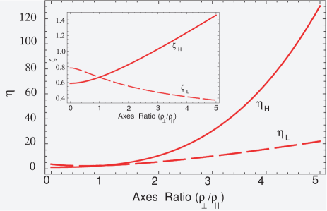
Figure 1: (Colour online) Dependence of the function $\eta$ on the particle axes ratio for the case of low $\omega<\upsilon_{\text{F}}/(2R)$ (dashed lines) and high $\omega>\upsilon_{\text{F}}/(2R)$ (solid lines) frequencies. In the inset: the same dependence for the functions $\zeta$ for the same frequency intervals.

It remains to consider the low frequency case. The next approximations are applied in this case in the calculus of equation (3.2)

$$\mathop{\symoperators Re}\nolimits{\left\{{{\frac{\psi_{1}(\upsilon^{\prime},\omega)}{{\nu-\mathrm{i}\omega}}}}\right\}}\approx{\frac{R}{{3\,\upsilon^{\prime}}}}\,,\qquad\mathop{\symoperators Re}\nolimits{\left\{{{\frac{\psi_{3}(\upsilon^{\prime},\omega)}{{\nu-\mathrm{i}\omega}}}}\right\}}\approx{\frac{R}{{36\,\upsilon^{\prime}}}}.$$ (3.31)

The procedure of simple but cumbersome calculations leads us to the next result

$$w_{\text{m}}^{\text{LF}}=\frac{3}{32}V\frac{\omega_{\text{pl}}^{2}}{4\piup\,c^{2}}\frac{\rho_{\bot}^{3}}{\upsilon_{\text{F}}}\int\limits_{0}^{\nu_{\text{S}}}\left\{\eta_{\text{L}}(e_{s})\;\xi^{2}|{\bf H}(0,\omega)|^{2}+\left[\zeta_{\text{L}}(e_{s})-\eta_{\text{L}}(e_{s})\;\xi^{2}\right]|{\bf H}(0,\omega)\,{\bf n}|^{2}\right\}\frac{\mathrm{d}\omega}{2\piup}\,,$$ (3.32)

where $\zeta_{\text{L}}(e_{s})$ and $\eta_{\text{L}}(e_{s})$ are some functions dependent on the spheroid eccentricity $e_{s}$. Their analytical form can be found in [20] (equations (55) and (97), with replacing $\zeta_{\text{L}}\to\rho_{\text{L}}$). In the inset of figure 1, the behaviour of these functions are shown as well. For a spherical particle, $\xi=1/2$, $\zeta_{\text{L}}(0)=\zeta_{\text{H}}(0)=2/3$, and $\eta_{\text{L}}(0)=\eta_{\text{H}}(0)=8/3$.

The calculation of equation (3.32) needs the estimation of the integral $I_{\text{L}}={\int_{0}^{\nu_{\text{S}}}{\omega^{2}f(\omega)}}\mathrm{d}\omega$, where $f(\omega)$ is given by equation (3.17). As it was shown in [22], the input of this integral is much less than the $I_{\nu_{\text{S}}}$ and one can neglect the first LF-term in the sum of equation (3.25) compared with the second one. For an arbitrary angle $\theta$ between the direction of the magnetic field and the spheroid rotation axis, we finally obtain

$$w_{\text{m}}=w_{\text{m}}^{\text{LF}}+w_{\text{m}}^{\text{HF}}=\frac{9}{64}\frac{V}{\sqrt{2\piup}}\frac{\omega_{\text{pl}}^{2}}{16\,c^{2}}\frac{\upsilon_{\text{F}}}{\Gamma}\left(1+\mathrm{e}^{-\frac{\omega_{\text{c}}^{2}}{2\Gamma^{2}}}\right)\rho_{\bot}\left[\zeta_{\text{H}}(e_{s})\cos^{2}\theta+\eta_{\text{H}}(e_{s})\,\xi^{2}\sin^{2}\theta\right]|{\bf H}_{0}|^{2},$$ (3.33)

where it is accounted that ${\bf H}_{\|}={\bf H}_{0}\cos\theta$ and ${\bf H}_{\bot}={\bf H}_{0}\sin\theta$. For spherical MN, equation (3.33) is simplified to

$$w_{\text{m}}=\frac{3}{64}\frac{VR}{\sqrt{2\piup}}\frac{\omega_{\text{pl}}^{2}}{8\,c^{2}}\frac{\upsilon_{\text{F}}}{\Gamma}\left(1+\mathrm{e}^{-\frac{\omega_{\text{c}}^{2}}{2\Gamma^{2}}}\right)\,|{\bf H}_{0}|^{2}.$$ (3.34)

The results of equations (3.19) and (3.21) obtained in the Drude approach transform into the results for the spheroidal particle given by equations (3.29) and (3.30) or equation (3.33) obtained in the kinetic approach, if we carry out a formal replacement

$${\begin{array}[]{*{20}c}{\nu\to\displaystyle\frac{45}{64}\frac{\upsilon_{\text{F}}}{\rho_{\bot}}\xi\eta_{\text{H}}\qquad\mbox{for}}\,\bot{\mbox{-polarization}},\vspace{1ex}\hfill\\ {\nu\to\displaystyle\frac{45}{32}\frac{\upsilon_{\text{F}}}{\rho_{\bot}}\zeta_{\text{H}}\qquad\mbox{for}\,\|\mbox{-polarization}\hfill}\\ \end{array}}$$ (3.35)

under a common condition $\omega\gg\nu$. Obviously, in the case of a spherical particle, the above replacement will look like:

$$\nu\to{\frac{15}{16}}{\frac{\upsilon_{\text{F}}}{R}}\,,\quad\mbox{provided that}\ \omega\gg\nu.$$ (3.36)

4 Discussion of results

The energy of a magnetic absorption of a plane EM-wave by a spherical MN per unit time in a classical case can be written as [25]

$$w_{\text{cl}}=\frac{1}{80}\frac{V}{\piup}\omega\,\varepsilon^{\prime\prime}\left(\frac{\omega R}{c}\right)^{2}{|{\bf H}_{0}|^{2}},$$ (4.1)

where

$$\varepsilon^{\prime\prime}=\frac{\nu}{\omega}\frac{\omega^{2}_{\text{pl}}}{\omega^{2}+\nu^{2}}.$$ (4.2)

For the frequency domain of $\omega\gg\nu$, equation (4.1) takes the form

$$w_{\text{cl}}=\frac{V}{80\piup}\left(\frac{\omega_{\text{pl}}R}{c}\right)^{2}{|{\bf H}_{0}|^{2}},$$ (4.3)

and the magnetic absorption of a plane EM-wave by a spherical MN does not depend on the wave frequency.

Let us illustrate the previous analytical expressions graphically. We calculate the ratio between the energy of a magnetic field absorbed by the spheroidal MN from the laser pulses per unit time, and the energy absorbed by the spherical MN from the magnetic component of the plane EM-wave

$$S_{\text{m}}=\frac{w_{\text{m}}}{w_{\text{cl}}}.$$ (4.4)

We limit ourselves only to the frequency interval $\nu\ll\omega\ll\omega_{\text{pl}}$.

While studying the dependence of the optical properties of the MNs on its shape, makes sense to compare the absorption in MNs with different shapes, but equal in volume. We modify the shape of a particle by changing the aspect ratio of the spheroid. The condition on the fixed volume of a particle ($V={\frac{4\piup}{3}}\rho_{\bot}^{2}\rho_{\|}=\text{const}$) with a given aspect ratio defines the values of $\rho_{\bot}$ and $\rho_{\|}$. For example, $\rho_{\bot}=R(\rho_{\bot}/\rho_{\|})^{1/3}$, where $R$ is the radius of the sphere of an equivalent volume [19].

Below, we will study the effect of the MN shape on the magnitude of the absorption energy of the magnetic component of the laser field for two different polarizations of this field (across and along the spheroid’s rotation axis). The shape of the particle will be determined by the spheroid aspect ratio. In figures 2 and 3, the dependence of $S_{\text{m}}$ on the degree of flattening or elongation of the spheroidal particle is depicted for two polarizations of the magnetic field (at the frequency of the surface plasmon $\omega_{\text{c}}=\omega_{\text{pl}}/\sqrt{3}$).

Figure 2: (Colour online) Dependence of the energy absorbed by a spheroidal metal nanoparticle with the polarization of the magnetic field transverse ($\bot$) to its axis of rotation on the spheroid aspect ratio. Bold lines are for oblate MN and dashed lines correspond to the prolate MN. The curves are built for a particle whose volume is equal to the volume of a spherical particle with a radius $R=100$ Å, and for different $\Gamma$: $2\cdot 10^{14}$ s^-1 (curve 1), $3\cdot 10^{14}$ s^-1 (2), $4\cdot 10^{14}$ s^-1 (3). The plot of the Drude dependence at $\Gamma=2\cdot 10^{14}$ s^-1 is given by thin curves 4.

Figure 3: (Colour online) The same as in figure 2 for $\|$-polarization of the magnetic field.

Calculations were carried out using equations (3.33), (4.3) and (4.4) with parameters close to the Au [26]: $n=5.9\cdot 10^{22}$ cm^-3, $\upsilon_{\text{F}}\approx 1.39\cdot 10^{8}$ cm/s, $\omega_{\text{pl}}\approx 1.37\cdot 10^{16}$ s^-1, and $\nu_{0^{\circ}\text{C}}=3.39\cdot 10^{13}$ s^-1. Curves 1–3 correspond to the different duration of the incident pulse. The dependences of $S_{\text{m}}$ in the Drude approach constructed on the basis of equations (3.19) and (3.21) are depicted by thin solid and dashed curves 4, respectively. By comparing curves 1–3, we can see that the energy of laser pulses with increasing duration is absorbed to a greater degree.

As one can see in figure 2 for the transverse polarization of the magnetic field ($\theta=\piup/2$, $\bot$-polarization), the magnetic absorption by the oblate MN increases, reaches a maximum at certain values of the aspect ratio and then decreases. In the Drude case, this maximum is achieved for particles of the elongated shape at $c/a=\sqrt{2}$, and in the kinetic case — at $c/a\approx 2$.

For the MN with a radius, for example, 100 Å, one can make sure that the absorption in the kinetic case is almost half the order of magnitude larger (compare, e.g., curves 1 and 4 in figure 2).

For the prolate MN in this polarization, the magnetic absorption decreases only with the aspect ratio growth.

If we compare the magnitudes of absorption for the spherical MN that can be obtained in the Drude and kinetic approaches [equations (3.19) and (3.29)] for the same pulse duration, then we will find

$${\left.{{\frac{w^{\text{HF}}_{\text{m}\bot}}{w_{\text{m}\bot}}}}\right|}_{\max}={\frac{15}{16}}\frac{\upsilon_{\text{F}}}{\nu R}.$$ (4.5)

From equation (4.5) it follows that this ratio increases with a decrease in the radius of the particle and does not depend on $\Gamma$.

In the polarization of the magnetic field along the spheroid axis of rotation ($\theta=0$, $\|$-polarization), the magnitude of the absorption increases (see figure 3) for an increasingly flattened MN and decreases with the growth of its elongation.

The reason for this is the fact that the number of closed electron orbits with an increasing flattening of the particle increases for $\|$- and falls for $\bot$-polarization of the magnetic field.

In contrast to the electric absorption, with the deviation of the carrier frequency from the frequency of the surface plasmon in a spherical particle, the maximum in the dependence of the absorbed energy on the aspect ratio is not displaced, and the other maxima associated with the particle shape do not appear. This fact takes place for both polarizations just as in the Drude, and in the kinetic descriptions of the process. However, depending on the duration of the incident pulse, there is a certain specificity. With an increase of the pulse duration, the absorption intensity increases at different carrier frequencies in the both polarizations.

As follows from equations (3.21) and (3.34), the energy absorbed by the spherical MN slightly depends on the ratio of $\Gamma/\omega_{\text{c}}$ in both the Drude and kinetic cases. Note that the spatial dimension of the pulse $c/\Gamma$ must not exceed the length of the carrier wave in a vacuum: $\Gamma/\omega_{\text{c}}\geqslant 1/(2\piup)\approx 0.16$.

Thus, the absorption in non-spherical particles essentially depends on the polarization of the magnetic field relative to the particle. The magnetic absorption in the spheroidal MN at $\bot$-polarization of the field weakly increases (in comparison with the spherical particles) in the flattened particles and falls in the elongated particles of the same volume. In the Drude approach, the absorption obtained in this polarization for both elongated and flattened particles is less than the one for the spherical particle. It is the smallest for particles with an elongated shape.

In the case of $\|$-polarization, the absorption markedly increases in the flattened and decreases in the elongated MN in comparison with the spherical MN. The same trends are observed in the Drude approach.

Thus, the spheroidal elongated or flattened MN in comparison with spherical ones can absorb the energy of the magnetic field of ultrashort laser pulses more or less intensively depending on the orientation of the magnetic field relative to the spheroid rotational axis.

A similar study for electrical absorption was carried out by us in [20].

From equations (3.19) and (3.29), or equations (3.21), (3.30), one can only see that the energy of the magnetic absorption under the Drude description grows as a square of $\rho_{\bot}$, whereas in the kinetic description, the growth takes place linearly with $\rho_{\bot}$.

5 Conclusions

The theory of the surface and shape influence on the dipole magnetic absorption of ultraviolet laser pulses by metal nanoparticles is developed for the cases when the electron mean free path exceeds or is less than the particle size.

The obtained analytical expressions allow one to study the magnetic absorption of pulses depending on their duration, shape of the particle, and polarization of the magnetic field. They are suitable in a wide range of applications. The correspondence between the results obtained in the Drude and kinetic approaches is discussed.

The absorption in non-spherical particles essentially depends on the polarization of the magnetic field relative to the particle. Thus, for the spheroidal MN, with the direction of the magnetic field across the spheroid rotation axis, the absorption increases in the flattened and falls in the elongated MN in comparison with the particles of a spherical shape of the same volume. In the case of the orientation of the magnetic field along the axis of the particle rotation, the situation is more pronounced compared with the spherical MN: the absorption appreciably increases in the flattened and falls in the elongated MN.

It is established that the energy of laser pulses with an increasing duration is absorbed to a greater extent. For any pulse duration, one can reveal the following tendency: at the transverse ($\bot$) polarization of the magnetic field, the absorption increases for the increasingly flattened MN, reaching the maximum at the spheroid aspect ratio $a/c\approx 2$, and then decreases with the greater aspect ratio. At the longitudinal polarization ($\|$) of the magnetic field, the absorption by flattened MN only increases with the flattening of the MN.

For particles of the elongated shape with an increasing elongation of the particle, the absorption decreases at both the $\bot$- and the $\|$-polarization of the magnetic field.

These tendencies maintain for the Drude description of the processes as well.

For the fixed pulse duration and with the both polarizations ($\|$ and $\bot$) of the magnetic field, the value of the magnetic absorption obtained in the kinetic approach for particles with $R=100$ Å can be half an order of magnitude higher than the corresponding values derived from the Drude approach.

Our results make it possible to control the effects of the nanoparticle surface and the shape on the magnetic absorption of ultrashort laser pulses by varying the particle shape, the duration of a laser pulse and with changing its polarization.

Ukrainian 0

Вплив поверхнi й форми наночастинки на дипольне магнiтне поглинання ультракоротких лазерних iмпульсiв М.I. Григорчук

             
Iнститут теоретичної фiзики iм. М.М. Боголюбова НАН України,
вул. Метрологiчна, 14-б, 03143 Київ, Україна

References

- [1] Akhmanov S.A., Vysloukh V.A., Chirkin A.S., Optics of Femtosecond Laser Pulses, AIP-Press, New-York, 1992.
-
[2]
Chung Y., Jones C.K.R.T., Schäfer T., Wayne C.E.,
Nonlinearity, 2005, 18, 1351–1374,
doi:10.1088/0951-7715/18/3/021. -
[3]
Boyer D., Tamarat P., Maali A., Lounis B., Orrit M.,
Science, 2002, 297, 1160–1163,
doi:10.1126/science.1073765. - [4] Anker J.N., Hall W.P., Lyandres O., Shah N.C., Zhao J., Van Duyne R.P., Nat. Mater., 2008, 7, 442–453, doi:10.1038/nmat2162.
- [5] Chen Y.T., Kolhatkar A.G., Zenasni O., Xu S., Lee T.R., Sensors, 2017, 17, 2300, doi:10.3390/s17102300.
- [6] Lee H., Shin T.-H., Cheon J., Weissleder R., Chem. Rev., 2015, 115, 10690–10724, doi:10.1021/cr500698d.
- [7] Arbouet A., Christofilos D., Del Fatti N., Vallée F., Huntzinger J.R., Arnaud L., Billaud P., Broyer M., Phys. Rev. Lett., 2004, 93, 127401, doi:10.1103/PhysRevLett.93.127401.
-
[8]
Wilkinson M., Mehlig B., Walker P.N.,
J. Phys.: Condens. Matter, 1998, 10, 2739–2758,
doi:10.1088/0953-8984/10/12/013. - [9] Deepika, Chauhan P., Varshney A., Singh D.B., Sajal V., J. Phys. D: Appl. Phys., 2015, 48, 345103, doi:10.1088/0022-3727/48/34/345103.
- [10] Asenjo-Garcia A., Manjavacas A., Myroshnychenko V., García de Abajo F.J., Opt. Express, 2012, 20, 28142–28152, doi:10.1364/OE.20.028142.
- [11] Cheng J.P., Roy R., Agrawal D., J. Mater. Sci. Lett., 2001, 20, 1561–1563, doi:10.1023/A:1017900214477.
- [12] Evlyukhin A.B., Novikov S.M., Zywietz U., Eriksen R.L., Reinhardt C., Bozhevolnyi S.I., Chichkov B.N., Nano Lett., 2012, 12, 3749–3752, doi:10.1021/nl301594s.
- [13] Kuznetsov A., Miroshnichenko A., Brongersma M., Kivshar Y., Luk’yanchuk B., Science, 2016, 354, aag2472, doi:10.1126/science.aag2472.
- [14] Goel D., Chauhan P., Varshney A., Singh D.B., Sajal V., In: Plasma and Fusion Science, Raneesh B., Kalarikkal N., James J., Nair A.K. (Eds.), Apple Academic Press, Oakville, 2009, 219–230.
- [15] Kelly K.L., Coronado F., Zhao L.L., Schatz G.C., J. Phys. Chem. B, 2003, 107, 668–677, doi:10.1021/jp026731y.
- [16] Grigorchuk N.I., EPL, 2018, 121, 67003, doi:10.1209/0295-5075/121/67003.
- [17] Bohren C.F., Huffman D.R., Absorption and Scattering of Light by Small Particles, Wiley, Weinheim, 2004.
- [18] Apiyo D., Schasfoort R., Schuck P., Marquart A., Gedig E.T., Karlsson R., Abdiche Y.N., Eckman J., Blum S.R., Schasfoort R.B.M., Handbook of Surface Plasmon Resonance, Royal Society of Chemistry, Cambridge, 2017.
- [19] Grigorchuk N.I., Condens. Matter Phys., 2013, 16, 33706, doi:10.5488/CMP.16.33706.
- [20] Tomchuk P.M., Grigorchuk N.I., Phys. Rev. B, 2006, 73, 155423, doi:10.1103/PhysRevB.73.155423.
- [21] Grigorchuk N.I., Tomchuk P.M., Low Temp. Phys., 2005, 31, 411–418, doi:10.1063/1.1925368.
- [22] Grigorchuk N.I., Tomchuk P.M., Phys. Rev. B, 2009, 80, 155456, doi:10.1103/PhysRevB.80.155456.
- [23] Bremermann H., Distribution, Complex Variables and Fourier Transforms, Pearson Education, New Jersey, 1965.
-
[24]
Kuznetsova I.A., Lebedev M.E., Yushkanov A.A.,
Tech. Phys., 2015, 60, 1261–1267,
doi:10.1134/S1063784215090091. - [25] Landau L.D., Lifshitz E.M., Electrodynamics of Continuous Media, Pergamon Press, Oxford, 1986.
- [26] Kittel Ch., Introduction to Solid State Physics, Wiley, New York, 1974.
Ukrainian \adddialect\l@ukrainian0 \l@ukrainian