PyStokes: phoresis and Stokesian hydrodynamics in Python

Abstract

We present a modular Python library for computing many-body hydrodynamic and phoretic interactions between spherical active particles in suspension, when these are given by solutions of the Stokes and Laplace equations. Underpinning the library is a grid-free methodology that combines dimensionality reduction, spectral expansion, and Ritz-Galerkin discretization, thereby reducing the computation to the solution of a linear system. The system can be solved analytically as a series expansion or numerically at a cost quadratic in the number of particles. Suspension-scale quantities like fluid flow, entropy production, and rheological response are obtained at a small additional cost. The library is agnostic to boundary conditions and includes, amongst others, confinement by plane walls or liquid-liquid interfaces. The use of the library is demonstrated with six fully coded examples simulating active phenomena of current experimental interest.

I Introduction

PyStokes is a Python library for studying phoretic and hydrodynamic interactions between spherical particles when these interactions can be described by the solutions of, respectively, the Laplace and Stokes equations. The library has been specifically designed for studying these interactions in suspensions of active particles, which are distinguished by their ability to produce flow, and thus motion, in the absence of external forces or torques. Such particles are endowed with a mechanism to produce hydrodynamic flow in a thin interfacial layer, which may be due to the motion of cilia, as in microorganisms (Brennen and Winet, 1977) or osmotic flows of various kinds in response to spontaneously generated gradients of phoretic fields (Ebbens and Howse, 2010). The latter, often called autophoresis, is a generalisation of well- known phoretic phenomena including, inter alia, electrophoresis (electric field), diffusiophoresis (chemical field) and thermophoresis (temperature field) that occur in response to externally imposed gradients of phoretic fields (Anderson, 1989).

Hydrodynamic and phoretic interactions between “active particles” in a viscous fluid are central to the understanding of their collective dynamics (Ebbens and Howse, 2010; Zhang et al., 2017). Under experimentally relevant conditions, the motion of the fluid is governed by the Stokes equation and that of the phoretic field, if one is present, by the Laplace equation. The “activity” appears in these equations as boundary conditions on the particle surfaces that prescribe the slip velocity in the Stokes equation and flux of the phoretic field in the Laplace equation. The slip velocity and the phoretic flux are related by a linear constitutive law that can be derived from a detailed analysis of the boundary layer physics (Anderson, 1989). The Stokes and Laplace equations are coupled by this linear constitutive law only at the particle boundaries. The linearity of the governing equations and of the coupling boundary conditions allows for a formally exact solution of the problem of determining the force per unit area on the particle surfaces. This formally exact solution can be approximated to any desired degree of accuracy by a truncated series expansion in a complete basis of functions on the particle boundaries. This, in turn, leads to an efficient and accurate numerical method for computing hydrodynamic and phoretic interactions between active particles (Singh et al., 2015; Singh and Adhikari, 2018; R. Singh et al., 2019).

The principal features that set this method apart are (a) the restriction of independent fluid and phoretic degrees of freedom to the particle boundaries (b) the freedom from grids, both in the bulk of the fluid and on the particle boundaries and (c) the ability to handle, within the same numerical framework, a wide variety of geometries and boundary conditions, including unbounded volumes, volumes bounded by plane walls or interfaces, periodic volumes and, indeed, any geometry-boundary condition combination for which the Green’s functions of the governing equations are simply evaluated.

The purpose of this article is to demonstrate the power of the numerical method, as implemented in Python library, through six fully coded examples that simulate experimental phenomena. Our software implementation uses a polylgot programming approach that combines the readability of Python with the speed of Cython and retains the advantages of a high-level, dynamically typed, interpreted language without sacrificing performance.

Our presentation is in the style of literate programming and draws inspiration from similar articles by Weideman and Reddy (Weideman and Reddy, 2000), Higham (Higham, 2001), and Trefethen (Trefethen, 2000). The article is best read alongside installing the library and executing the example codes. The library freely is available on GitHub at https://github.com/rajeshrinet/pystokes,  where detailed installation instructions can also be found. A subset of the library features is available as a Binder file which requires no installation. All software is released under the MIT license.

The remainder of the paper consists of sections where each of the examples are explained in detail and a concluding section on features of the library not covered in the examples, features that can be added but have not been, and limitations of the numerical method. We end this Introduction with a brief description of each of the examples. In Section IV we compute the flows produced by the leading terms of the spectral expansion of the active slip for a single spherical particle away from boundaries. In Section V, we examine the effect of boundaries - a plane wall and a plane liquid-liquid interface - and show how the flows in the first example are altered. In Section VI we simulate the Brownian motion of a pair of hydrodynamically interacting active particles in a thermally fluctuating fluid confined by a plane wall. We identify an attractive drag force from the active flow and an unbinding transition with increasing temperature as entropic repulsion overwhelms this active hydrodynamic attraction. In Section VII we simulate the flow-induced phase separation (FIPS) of active particles at a plane wall. This provides a quantitative description of the crystallization of active particles that swim into a wall (Theurkauff et al., 2012; Palacci et al., 2013; Buttinoni et al., 2013; Chen et al., 2015; Petroff et al., 2015; Thutupalli et al., 2018; Aubret et al., 2018). In Section IV we introduce a phoretic flux on the particle surface and compute the phoretic field that it produces, both away from and in the proximity of a no-flux wall. In Section IX, we show that a competition between the hydrodynamic and phoretic interactions of autophoretic particles can arrest the phase separation induced by flow alone (R. Singh et al., 2019). In the penultimate section, we show that the cost of computation increases quadratically with the number of particles and decreases linearly with the number of computational threads.

II Mathematical underpinnings

Our method relies on the reduction of linear elliptic partial differential equations (PDE) to systems of linear algebraic equations. The four key mathematical steps underpinning it are illustrated in this diagram:

$$\boxed{\text{elliptic PDE}\xrightarrow{\,\,1\,\,}\text{boundary integral}\xrightarrow{\,\,2\,\,}\text{spectral expansion}\xrightarrow{\,\,3\,\,}\text{Ritz-Galerkin discretization}\xrightarrow{\,\,4\,\,}\text{truncation}}$$

The first step is the representation of the solution of an elliptic PDE in a three-dimensional volume $V$ as an integral over the boundary of the volume $S$ (Odqvist, 1930; Ladyzhenskaia, 1969; Youngren and Acrivos, 1975; Zick and Homsy, 1982; Pozrikidis, 1992; Muldowney and Higdon, 1995; Cheng and Cheng, 2005; Singh et al., 2015). For the Laplace equation, this is the classical theorem of Green (Jackson, 1962); for the Stokes equation, it is the generalization obtained by Lorentz (Odqvist, 1930; Lorentz, 1896; Ladyzhenskaia, 1969). The integral representation leads to a linear integral equation that provides a functional relation between the field and its flux on $S$. Thus, if the surface flux in the Laplace equation is specified, the surface concentration is determined by the solution of the Laplace boundary integral equation. Similarly, if the surface velocity in the Stokes equation is specified, the surface traction is determined by the solution of the Stokes boundary integral equation. This transformation of the governing PDEs is the most direct way of relating boundary conditions (surface flux, slip velocities) to boundary values (surface concentration, surface traction). It reduces the dimensionality of the problem from a three-dimensional one in $V$ to a two-dimensional one on $S$. The second step is the spectral expansion of the field and its flux in terms of global basis functions on $S$. We use the geometry-adapted tensorial spherical harmonics, which provide an unified way of expanding both scalar and vector quantities on the surface of a sphere. These functions are both complete and orthogonal and provide representations of the three-dimensional rotation group (Hess, 2015). Thus, symmetries of the active boundary conditions can be represented in a straightforward and transparent manner. The third step is the discretization of the integral equation using the procedure of Ritz and Galerkin (Boyd, 2000; Finlayson and Scriven, 1966), which reduces it to an infinite-dimensional self-adjoint linear system in the expansion coefficients. This exploits the orthogonality of the basis functions on the sphere. The matrix elements of the linear system can be evaluated analytically in terms of the Green’s functions of the respective elliptic equations. The fourth step is the truncation of the infinite-dimensional linear system to a finite-dimensional one that can be solved by standard methods of linear algebra adapted for self-adjoint systems (Saad, 2003). Analytical solution can be obtained by Jacobi iteration, which is equivalent to Smoluchowski’s method of reflections. Numerical solutions can be obtained by the conjugate gradient method, at a cost quadratic in the number of unknowns. From this solution, we can reconstruct the field and the flux on the boundary, use these to determine the fields in the bulk, and from there, compute derived quantities. These steps have been elaborated in several papers (Ghose and Adhikari, 2014; Singh et al., 2015; Singh and Adhikari, 2016, 2018; R. Singh et al., 2019) and we do not repeat them in detail here. Instead, we show below how the method is applied to problems of experimental interest.

III Library structure

The overall organization of the library is show in Table 1 and will be referred to throughout the remainder of the paper. The PyStokes library solves, respectively, the Stokes and Laplace equations, using the reduction method explained in the previous section. The library takes as input a set of expansion coefficients $\mathbf{J}_{i}^{(l)}$ for the prescribed active flux $j^{A}$ on the surface of the $i$-th particle and computes the expansion coefficients of the surface concentration. The active slip velocity $\boldsymbol{v}^{\mathcal{A}}$ is obtained from this using the linear coupling relation $\boldsymbol{v}^{\mathcal{A}}=\mu_{c}\boldsymbol{\nabla}_{s}c$ (Anderson, 1989). The library outputs the expansion coefficients $\mathbf{V}_{i}^{(l\sigma)}$ of the active slip. The PyStokes library takes as input these expansion coefficients, which may also be specified independently, and any body forces $\mathbf{F}_{i}^{B}$ and body torques $\mathbf{T}_{i}^{B}$ acting on the particles and returns their rigid body motion in terms of the velocities $\mathbf{V}_{i}$ and angular velocities $\boldsymbol{\Omega}_{i}$. In addition to the joint computation of phoretic and hydrodynamic interactions, the PyStokes library can be used to compute the hydrodynamically interacting motion of squirming particles where the slip is specified independently of a phoretic field, or the dynamics of passive sus- pensions where the slip vanishes and forces and torques are prescribed. The PyStokes library can also compute hydrodynamically correlated Brownian motion, and thus, allows the study of the interplay between passive, active, and Brownian contributions to motion. The library optionally computes the corresponding field in $V$, necessary for insight and visualization. Additionally, PyStokes computes the dissipation of mechanical energy and the rheological response of the suspension.

Table 1: This schematic shows the governing equations that determine the hydrodynamic and phoretic interactions between active particles in a three-dimensional domain $V$. The equations are coupled by the active boundary conditions on the surface $S_{i}$ of the $i$-th particle. The library takes as input surface fluxes $j^{\mathcal{A}}$, specified in terms of coefficients $\mathbf{J}_{i}^{(l)}$ of its tensorial harmonic expansion, and returns slip velocities $\boldsymbol{v}^{\mathcal{A}}$ specified in terms of coefficients $\mathbf{V}_{i}^{(l\sigma)}$ of its tensorial harmonic expansion. To solve the Stokes part of the problem, the library takes input these slip velocities and possible body forces $\mathbf{F}_{i}^{B}$ and torques $\mathbf{T}_{i}^{B}$ and returns the velocities $\mathbf{V}_{i}$ and angular velocities $\boldsymbol{\Omega}_{i}$. With slip velocities set to zero, PyStokes computes the hydrodynamically interacting motion of passive particles. Each library additionally computes the corresponding fields in the bulk and quantities derived from these, like the entropy production and rheological response. Particle indices are $i=1,\ldots,N$ and harmonic indices are $l=1,2,\ldots$ and $\sigma=s,a,t$ (see text).

IV Example 1 - Irreducible Active flows

Our first example shows how to plot the irreducible parts of an active flow around a spherical particle, which we take to be far removed from boundaries. For this example, we will take the reader step by step from the governing PDE to the expressions for the irreducible flows that the PyStokes library evaluates and plots.

1. Elliptic PDE. The flow field $\boldsymbol{v}(\boldsymbol{r})$ satisfies the Stokes equation in the region $V$ exterior to the sphere (radius $b$, centered at $\boldsymbol{R}$, oriented along unit vector $\boldsymbol{p}$). On the sphere surface $S,$ it satisfies the slip boundary condition

   $$\lim_{\boldsymbol{r}\rightarrow S}\boldsymbol{v}(\boldsymbol{r})=\mathbf{V}+\boldsymbol{\Omega}\times\boldsymbol{\rho}+\boldsymbol{v}^{\mathcal{A}}(\boldsymbol{\rho)},$$ (1)

   where $\mathbf{V}$ and $\boldsymbol{\Omega}$ are the rotational and translational velocities of the sphere, $\boldsymbol{v}^{\mathcal{A}}(\boldsymbol{\rho})$ is the slip velocity and and $\boldsymbol{\rho}$ is the radius vector from the center to $S$. The fundamental solution of the Stokes equation is given by the system

   $$-\nabla_{\alpha}P_{\beta}+\eta\nabla^{2}G_{\alpha\beta}=-\delta\left(\boldsymbol{r}-\boldsymbol{r^{\prime}}\right)\delta_{\alpha\beta},$$ (2a)

   $$K_{\alpha\beta\gamma}=-\delta_{\alpha\gamma}P_{\beta}+\eta\left(\nabla_{\gamma}G_{\alpha\beta}+\nabla_{\alpha}G_{\beta\gamma}\right),\quad\nabla_{\alpha}G_{\alpha\beta}=0.$$ (2b)

   where $G_{\alpha\beta}$ is the Green’s function, $P_{\alpha}$ is the pressure vector, $K_{\alpha\beta\gamma}$ is the fundamental solution for the stress tensor, and $\eta$ is the fluid viscosity. The Green’s function may need to satisfy additional boundary conditions which we keep unspecified for now.

2. Boundary integral. The fundamental solution, together with the Lorentz reciprocal relation gives the boundary integral representation

   $$v_{\alpha}(\boldsymbol{r})=-\int G_{\alpha\beta}(\boldsymbol{r},\boldsymbol{R}+\boldsymbol{\rho})\,f_{\beta}(\boldsymbol{\rho})\,d\text{S} +\int K_{\beta\alpha\gamma}(\boldsymbol{r},\boldsymbol{R}+\boldsymbol{\rho})\hat{\rho}_{\gamma}v_{\beta}^{\mathcal{}}(\boldsymbol{\rho})\,d\text{S},$$ (3)

   which expresses the flow field in $V$ in terms of a “single-layer” integral involving the traction and a “double-layer” integral involving the boundary velocity. The latter is specified by the boundary condition; the former must be determined in terms of it.

3. Spectral expansion. The analytical evaluation of the two integrals is possible if the slip and the traction are expanded spectrally in terms of tensorial spherical harmonics,

   $$\boldsymbol{v}^{\mathcal{A}}(\boldsymbol{\rho})=\sum_{l=1}^{\infty}w_{l-1}\mathbf{V}^{(l)}\cdot\mathbf{Y}^{(l-1)}(\bm{\hat{\rho}}),\quad\boldsymbol{f}(\boldsymbol{\rho})=\sum_{l=1}^{\infty}\tilde{w}_{l-1}\mathbf{F}^{(l)}\cdot\mathbf{Y}^{(l-1)}(\bm{\hat{\rho}}),$$ (4)

   where ${\bf Y}^{(l)}(\boldsymbol{\hat{\rho}})=(-1)^{l}\rho^{l+1}\nabla^{l}\rho^{-1}$ is the $l$-th irreducible tensorial harmonic. The $l$-th rank tensorial coefficients $\mathbf{V}^{(l)}$ and $\mathbf{F}^{(l)}$ are symmetric and irreducible in their last $l-1$ indices and have the dimensions of velocity and force respectively. The dot indicates a complete contraction of the indices of ${\bf Y}^{(l)}$ with the contractible indices of the coefficients. The $l$-dependent expansion weights are $w_{l}=\frac{1}{l!(2l-1)!!}$ and $\tilde{w}_{l}=\frac{2l+1}{4\pi b^{2}}$. The orthogonality of the tensorial harmonics implies that

   $$\mathbf{V}^{(l)}=\tilde{w}_{l-1}\int\boldsymbol{v}^{\mathcal{A}}(\boldsymbol{R}+\bm{\rho})\mathbf{Y}^{(l-1)}(\bm{\hat{\rho}})d\text{S},\qquad\mathbf{F}^{(l)} =w_{l-1}\int\boldsymbol{f}(\boldsymbol{R}+\bm{\rho})\mathbf{Y}^{(l-1)}(\bm{\hat{\rho}})d\text{S}.$$ (5)

   The integral of the traction, $\mathbf{F}^{(1)}$, is the net hydrodynamic force and the integral of the cross-product of the traction with the radius vector, the antisymmetric part of ${\bf F}^{(2)},$ is the net hydrodynamic torque (Singh and Adhikari, 2018).

4. Ritz-Galerkin discretization. Letting the point $\boldsymbol{r}$ approach $S$ from $V$ and matching the flow in the integral representation with the prescribed boundary condition leads to an integral equation for the traction. Multiplying both sides of the integral equation by the $l$-th harmonic and integrating yields an infinite-dimensional system of linear equations for the coefficients of the traction,

   $$\tfrac{1}{2}\tilde{\mathbf{V}}^{(l)}=-\boldsymbol{G}^{(l,l^{\prime})}\cdot\mathbf{F}^{(l^{\prime})}+\boldsymbol{K}^{(l,l^{\prime})}\cdot\tilde{\mathbf{V}}^{(l)},$$ (6)

   where repeated indices are summed over, $\tilde{\mathbf{V}}^{(1)}=\mathbf{V}+\mathbf{V}^{(1)},$ $\tilde{\mathbf{V}}^{(2)}=b\mathbf{\boldsymbol{\epsilon}\cdot\boldsymbol{\Omega}}+\mathbf{V}^{(2)}$, $\tilde{\mathbf{V}}^{(l)}=\mathbf{V}^{(l)}$ for $l>2$, and $\boldsymbol{G}^{(l,\,l^{\prime})}$ and $\boldsymbol{K}^{(l,\,l^{\prime})}$ are the matrix elements of the linear system given in terms of integrals of the Green’s function and the fundamental stress solution. These can be evaluated analytically (Singh and Adhikari, 2018).

5. Truncation: The infinite-dimensional linear system has to be truncated to a finite-dimensional one for tractability. We truncate the system at $l=2$ and decompose the coefficients into their irreducible symmetric ($s)$, antisymmetric $(a)$ and trace $(t)$ parts, so that slip and the traction are

   $$\boldsymbol{v}^{\mathcal{A}}(\bm{\rho})=\mathbf{V}^{(1s)}+[\mathbf{V}^{(2s)}-\boldsymbol{\epsilon}\cdot\mathbf{V}^{(2a)}]\cdot\mathbf{Y}^{(1)}+\tfrac{1}{6}[\mathbf{V}^{(3s)}-\tfrac{2}{3}\boldsymbol{\Delta}\cdot(\boldsymbol{\boldsymbol{\epsilon}}\cdot\mathbf{V}^{(3a)})+\tfrac{3}{5}\boldsymbol{\Delta}\cdot(\boldsymbol{\delta}\mathbf{V}^{(3t)})]\cdot\mathbf{Y}^{(2)},$$ (7a)

   $$4\pi b^{2}\,\boldsymbol{f}(\bm{\rho})=\mathbf{F}^{(1s)}+3[\mathbf{F}^{(2s)}-\tfrac{1}{2}\boldsymbol{\epsilon}\cdot\mathbf{F}^{(2a)}]\cdot\mathbf{Y}^{(1)}+5[\mathbf{F}^{(3s)}-\tfrac{2}{3}\boldsymbol{\Delta}\cdot(\boldsymbol{\boldsymbol{\epsilon}}\cdot\mathbf{F}^{(3a)})+\tfrac{3}{5}\boldsymbol{\Delta}\cdot(\boldsymbol{\delta}\mathbf{F}^{(3t)})]\cdot\mathbf{Y}^{(2)}.$$ (7b)

   Here $\boldsymbol{\epsilon}$ and $\boldsymbol{\delta}$ are the Levi-Civita and Kronecker tensors and $\Delta_{\alpha\beta\mu\nu}=\tfrac{1}{2}(\delta_{\alpha\nu}\delta_{\beta\mu}+\delta_{\alpha\mu}\delta_{\beta\nu}-\frac{2}{3}\delta_{\alpha\beta}\delta_{\mu\nu})$ symmetrises and detraces second-rank tensors. This truncation includes all long-ranged contributions to the active flow and is sufficient to parametrize experimentally measured active flows around microorganisms, active drops, and autophoretic colloids (Ghose and Adhikari, 2014; Singh and Adhikari, 2016; Thutupalli et al., 2018). The solution of the finite-dimensional linear system yields a linear relation between the irreducible force and velocity coefficients, the “generalized Stokes laws”, which are $\mathbf{F}^{(l\sigma)}=-\boldsymbol{\gamma}^{(l\sigma,l^{\prime}\sigma^{\prime})}\cdot\tilde{\mathbf{V}}^{(l^{\prime}\sigma^{\prime})}$ where $\sigma=s,a,t$ and repeated indices are summed over. In an unbounded domain the friction tensors $\boldsymbol{\gamma}^{(l\sigma,l^{\prime}\sigma^{\prime})}$ take on a particularly simple form: they are diagonal in both the $l$ and $\sigma$ indices, $\boldsymbol{\gamma}^{(l\sigma,l^{\prime}\sigma^{\prime})}\equiv\delta_{ll^{\prime}}\delta_{\sigma\sigma^{\prime}}\gamma^{l\sigma}\Delta^{(l)}$ so that a single scalar $\gamma^{l\sigma}$ determines them. For $l\sigma=1s$ and $l\sigma=2a$ these are the familiar coefficients $6\pi\eta b$ and $8\pi\eta b^{3}$ that appear in Stokes laws for the force and torque.

⬇

# ex1.py - flow around an active colloid in an unbounded domain

import pystokes, numpy as np, matplotlib.pyplot as plt

# particle radius, fluid viscosity, and number of particles

b, eta, Np = 1.0, 1.0/6.0, 1

#initialise position, orientation and body force on the colloid

r, p, F = np.array([0.0, 0.0, 0.0]), np.array([0.0, -1.0, 0]), np.array([0.0, 1.0, 0])

# irreducible coeffcients

V2s = pystokes.utils.irreducibleTensors(2, p)

V3t = pystokes.utils.irreducibleTensors(1, p)

# space dimension , extent , discretization

dim, L, Ng = 3, 10, 100;

# instantiate the Flow class

flow = pystokes.unbounded.Flow(radius=b, particles=Np, viscosity=eta, gridpoints=Ng*Ng)

# plot using subplots on a grid

rr, vv = pystokes.utils.gridXY(dim, L, Ng)

plt.figure(figsize=(15, 10), edgecolor=’gray’, linewidth=4)

plt.subplot(231); vv=vv*0; flow.flowField1s(vv, rr, r, F)

pystokes.utils.plotStreamlinesXY(vv, rr, r, offset=6e-1, title=’1s’, density=2)

plt.subplot(232); vv=vv*0; flow.flowField2s(vv, rr, r, V2s)

pystokes.utils.plotStreamlinesXY(vv, rr, r, offset=4e-2, title=’2s’, density=2)

plt.subplot(233); vv=vv*0; flow.flowField3t(vv, rr, r, V3t)

pystokes.utils.plotStreamlinesXY(vv, rr, r, offset=4e-4, title=’3t’, density=2)

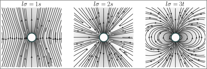
Figure 1: Irreducible flows: Streamlines of the fluid overlaid on the pseudocolor plot of the logarithm of the flow speed (increasing in strength from light to dark). The first panel is the flow due the $1s$ mode of the traction, the second and third panels are due to $2s$ and $3t$ modes of the active slip. The streamlines inherit the symmetry of the modes.

Inserting the truncated spectral expansions for the slip and traction in the boundary integral, eliminating the unknown traction coefficients in favour of the known slip coefficients, expanding the Green’s function about the center of the sphere and finally using the orthogonality of the tensorial harmonics, we obtain the flow due to each irreducible slip mode as

$$\text{}\boldsymbol{v}^{1s}(\boldsymbol{r})=-(1+\tfrac{b^{2}}{6}\nabla^{2})\,\mathbf{G}\cdot\mathbf{F}^{(1s)},$$ (8a)

$$\boldsymbol{v}^{2s}(\boldsymbol{r})=\tfrac{28\pi\eta b^{2}}{3}(1+\tfrac{b^{2}}{10}\nabla^{2})\,\boldsymbol{\nabla}\mathbf{G}\cdot\mathbf{V}^{(2s)},\qquad\boldsymbol{v}^{2a}(\boldsymbol{r})=-\frac{1}{2}(\boldsymbol{\nabla}\times\mathbf{G})\cdot\mathbf{F}^{(2a)},$$ (8b)

$$\boldsymbol{v}^{3s}(\boldsymbol{r})=\tfrac{13\pi\eta b^{3}}{9}(1+\tfrac{b^{2}}{14}\nabla^{2})\boldsymbol{\nabla}\boldsymbol{\nabla}\mathbf{G}\cdot\mathbf{V}^{(3s)},\quad\boldsymbol{v}^{3a}(\boldsymbol{r})=\tfrac{2\pi\eta b^{3}}{3}\boldsymbol{\nabla}(\boldsymbol{\nabla}\times\mathbf{G})\cdot\mathbf{V}^{(3a)},\quad\boldsymbol{v}^{3t}(\boldsymbol{r})=\tfrac{2\pi\eta b^{3}}{5}\nabla^{2}\mathbf{G}\cdot\mathbf{V}^{(3t)}.$$ (8c)

We emphasise that these expressions are valid for any Green’s function of the Stokes equation, provided they satisfy the additional boundary conditions that may be imposed. We also note that no discretization of space, either in $V$ or on $S$ is involved, making the result “grid-free”. The $\mathtt{flow}$ class in PyStokes computes these expressions for supplied values of the force, the torque and slip coefficients. For this example, we choose an unbounded domain with the flow vanishing at infinity, for which the Green’s function is the Oseen tensor,

$$G_{\alpha\beta}^{\text{o}}(\boldsymbol{r}-\boldsymbol{r}^{\prime})=\frac{1}{8\pi\eta}\left(\nabla^{2}\delta_{\alpha\beta}-\nabla_{\alpha}\nabla_{\beta}\right)|\boldsymbol{r}-\boldsymbol{r}^{\prime}|.$$ (9)

The code listed in Fig.(1) computes the irreducible flows $1s$, $2s,$ and $3t$ for radius $b=1$, viscosity $\eta=1/6$, location $\boldsymbol{R}=(0,0,0)$ and orientation $\boldsymbol{p}=(0,-1,0).$ The coefficients are parametrised as $F_{\alpha}^{(1s)}=-p_{\alpha},$ $V_{\alpha\beta}^{(2s)}=p_{\alpha}p_{\beta}-\frac{1}{3}\delta_{\alpha\beta}$ and $V_{\alpha}^{(3t)}=p_{\alpha}$. This information is supplied to the $\mathtt{flow}$ class which is instantiated for an unbounded fluid. The $l\sigma$ irreducible component of the flow is computed by the calling the function $\mathtt{flow.flowfieldl\sigma}$. This is passed to a generic plotting function to compute the streamlines in a plane of symmetry. These are shown in the code output where the polar symmetries of the $1s$ and $3t$ modes and the nematic symmetry of the $2s$ mode can be seen clearly. For vanishing radius, these are the Stokeslet, potential dipole and stresslet singularities (Batchelor, 2000).

⬇

# ex2.py - comparison of flow around an active colloid near a plane surface (wall and interface)

import pystokes, numpy as np, matplotlib.pyplot as plt

# particle radius, fluid viscosity, and number of particles

b, eta, Np = 1.0, 1.0/6.0, 1

#initialise position, orientation and body force on the colloid

r, p, F = np.array([0.0, 0.0, 3.4]), np.array([0.0, 0.0, 1]), np.array([0.0, 0.0, 1])

# irreducible coeffcients

V2s = pystokes.utils.irreducibleTensors(2, p)

V3t = pystokes.utils.irreducibleTensors(1, p)

# space dimension , extent , discretization

dim, L, Ng = 3, 10, 64;

# Instantiate the Flow class

wFlow = pystokes.wallBounded.Flow(radius=b, particles=Np, viscosity=eta, gridpoints=Ng*Ng)

iFlow = pystokes.interface.Flow(radius=b, particles=Np, viscosity=eta, gridpoints=Ng*Ng)

# plot using subplots on a given grid

plt.figure(figsize=(15, 8))

rr, vv = pystokes.utils.gridYZ(dim, L, Ng)

plt.subplot(231); vv=vv*0; wFlow.flowField1s(vv, rr, r, F)

pystokes.utils.plotStreamlinesYZsurf(vv, rr, r, mask=0.5, title=’1s’)

plt.subplot(232); vv=vv*0; wFlow.flowField2s(vv, rr, r, V2s)

pystokes.utils.plotStreamlinesYZsurf(vv, rr, r, mask=0.4, title=’2s’)

plt.subplot(233); vv=vv*0; wFlow.flowField3t(vv, rr, r, V3t)

pystokes.utils.plotStreamlinesYZsurf(vv, rr, r, mask=0.5, title=’3t’)

plt.subplot(234); vv=vv*0; iFlow.flowField1s(vv, rr, r, F)

pystokes.utils.plotStreamlinesYZsurf(vv, rr, r, mask=0.0, title=’None’)

plt.subplot(235); vv=vv*0; iFlow.flowField2s(vv, rr, r, V2s)

pystokes.utils.plotStreamlinesYZsurf(vv, rr, r, mask=0.0, title=’None’)

plt.subplot(236); vv=vv*0; iFlow.flowField3t(vv, rr, r, V3t)

pystokes.utils.plotStreamlinesYZsurf(vv, rr, r, mask=0.5, title=’None’)

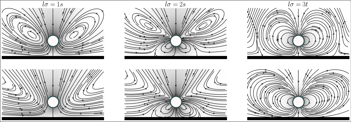
Figure 2: Distortion of irreducible flows, by a plane no-slip wall (top row) and plane no-shear interface (bottom row), due to the $1s$ mode of the traction and $2s$ and $3t$ modes of the active slip. The streamlines no longer inherit the symmetry of the modes.

V Example 2 - Effect of plane boundaries

Our second example illustrates how irreducible flows are modified by the proximity to plane boundaries. This is of relevance to experiments, where confinement by boundaries is commonplace (Goldstein, 2015; Thutupalli et al., 2018). This also illustrates the flexibility of our method, as the only quantity that needs to be changed is the Green’s function. The Green’s function for a no-slip wall is the Lorentz-Blake tensor

$$G_{\alpha\beta}^{\text{w}}(\boldsymbol{R}_{i},\,\boldsymbol{R}_{j}) = G_{\alpha\beta}^{\text{o}}(\boldsymbol{r}_{ij})-G_{\alpha\beta}^{\text{o}}(\boldsymbol{r}_{ij}^{*})-2h\nabla_{{\scriptscriptstyle\boldsymbol{r}_{\gamma}^{*}}}G_{\alpha 3}^{\text{o}}(\boldsymbol{r}_{ij}^{*})\mathcal{M}_{\beta\gamma}+h^{2}\nabla_{{\scriptscriptstyle\boldsymbol{r}^{*}}}^{2}G_{\alpha\gamma}^{\text{o}}(\boldsymbol{r}_{ij}^{*})\mathcal{M}_{\beta\gamma}.$$ (10)

Here $\boldsymbol{r}_{ij}^{*}=\mathbf{\boldsymbol{R}}_{i}-\mathbf{\boldsymbol{R}}_{j}^{*}$, where $\boldsymbol{R}_{j}^{*}=\boldsymbol{\mathcal{M}}\cdot\boldsymbol{R}$ is the image of the $j$-th colloid at a distance $h$ from plane boundary and $\boldsymbol{\mathcal{M}}=\boldsymbol{I}-2\mathbf{\hat{z}}\mathbf{\hat{z}}$ is the reflection operator. The Green’s function for a no-shear plane air-water interface is

$$G_{\alpha\beta}^{\text{i}}(\boldsymbol{R}_{i},\,\boldsymbol{R}_{j}) = G_{\alpha\beta}^{\text{o}}(\boldsymbol{r}_{ij})+(\delta_{\beta\rho}\delta_{\rho\gamma}-\delta_{\beta 3}\delta_{3\gamma})G_{\alpha\gamma}^{\text{o}}(\boldsymbol{r}_{ij}^{*}).$$ (11)

The plane boundary is placed at $z=0$ and the flows are plotted in the half-space $z>0$. The irreducible flows for each boundary condition are obtained by evaluated Eq.(8) with the corresponding Green’s function. The irreducible flows for the modes in Example 1 are shown in Fig.(2), with no-slip wall in the top panels and no-shear interface in the bottom panels. We use the same initialization as in Example 1, but instantiate wall-bounded and interfacially-bounded classes $\mathtt{wflow}$ and $\mathtt{iflow}$ respectively. Though arbitrary viscosity ratios are allowed, PyStokes assumes an air-water interface as default, setting the viscosity ratio between the two fluids to zero, as in this example. The $l\sigma$ irreducible component of the flow is computed by the calling the function $\mathtt{wflow.flowfieldl\sigma}$ and passed to a generic plotting function for streamline computation. Note that the streamlines near an interface do not close, unlike those near a plane wall. The perpendicular component of the flow near a wall is about an order of magnitude larger than that near an interface. These features have been recently used to understand the control by boundaries of flow-induced phase separation of active particles (Thutupalli et al., 2018).

VI Example 3 - Active Brownian Hydrodynamics

⬇

# ex3.py: competition between flow-induced forces and thermal fluctuations

import pystokes, numpy as np, matplotlib.pyplot as plt

# particle radius, self-propulsion speed, number and fluid viscosity

b, vs, Np, eta = 1.0, 0.5, 2, 0.1

rbm = pystokes.wallBounded.Rbm(radius=b, particles=Np, viscosity=eta)

forces = pystokes.forceFields.Forces(particles=Np)

def twoBodyDynamics(T=1):

"""simulation of two active colloid near a wall in a fluid at temperature T"""

#initial position and orientation

r, p = np.array([-2.5,2.5, 0,0 , 2.5, 2.5]), np.array([0,0, 0,0, -1.0,-1.0])

# integration parameters and arrays

Nt=2**17; x1=np.zeros(Nt); x2=np.zeros(Nt)

x1[0], x2[0] = r[0], r[1]; dt=0.01; sqdt=np.sqrt(T*dt)

F = np.zeros(3*Np); v = np.zeros(3*Np); vv = np.zeros(3*Np)

F0 = 6*np.pi*eta*b*vs*(1+9*b/(8*r[4])); #active stall force

# integration loop

for i in range(Nt-1):

forces.lennardJones(F,r,lje=.12,ljr=2.5); F[4],F[5]= F0, F0

rbm.mobilityTT(v, r, F); rbm.calcNoiseMuTT(vv, r)

# Euler-Maryuama integration

x1[i+1] = x1[i] + dt*v[0] + sqdt*vv[0]

x2[i+1] = x2[i] + dt*v[1] + sqdt*vv[1]

#reset the variables for next time step

r[0],r[1],v,vv,F[0:3] = x1[i+1], x2[i+1],v*0,vv*0,F[0:3]*0

return x1, x2

# dynamics as a function of temperature

T=([0, .1]); pystokes.utils.plotTrajectory(twoBodyDynamics, T)

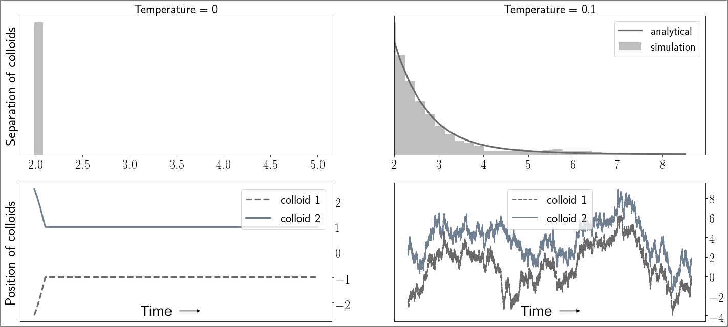
Figure 3: Fluctuating hydrodynamics of a pair of active particles near a plane wall. The two particles form a bound state in absence of thermal fluctuations. At finite temperatures, they “unbind” and distribution of their separation follows from an nonequilibrium potential (see text).

Our third example shows how to simulate the dynamics of active particles including active, passive and thermal forces. This example assumes that orientational degrees of freedom are not dynamical, as is often the case with strongly bottom-heavy active particles. The PyStokes library computes the rigid body motion of the active particles consistent with the overdamped Langevin equation

$$\mathbf{F}_{i}^{H}+\mathbf{F}_{i}^{B}+\hat{\mathbf{F}}_{i}=0,$$ (12)

where $\mathbf{F}_{i}^{H}=\mathbf{F}_{i}^{(1s)}$, $\mathbf{F}_{i}^{B}$ and $\hat{\mathbf{F}}_{i}$ are the hydrodynamic, body and thermal forces respectively and $i$ is the particle index. We now consider a minimal model of the slip, retaining only the lowest modes of vectorial symmetry:

$$\boldsymbol{v}^{\mathcal{A}}(\boldsymbol{\hat{\rho}}_{i})=\mathbf{V}_{i}^{(1s)}+\tfrac{1}{15}\mathbf{V}_{i}^{(3t)}\cdot\mathbf{Y}^{(2)}(\boldsymbol{\hat{\rho}}_{i}).$$ (13)

We parametrize the coefficients of the slip uniaxially, in terms of the orientation $\boldsymbol{p}_{i}$ of the $i$-th colloid and its self-propulsion speed $v_{s}$, as

$$\mathbf{V}_{i}^{(1s)}=v_{s}\,\boldsymbol{p}_{i},\qquad\mathbf{V}_{i}^{(3t)}=V_{0}^{(3t)}\,\boldsymbol{p}_{i}.$$ (14)

The hydrodynamic forces are then given by the generalized Stokes laws,

$$\mathbf{F}_{i}^{H}= -\boldsymbol{\gamma}_{ij}^{TT}\cdot(\mathbf{V}_{j}+\mathbf{V}_{j}^{(1s)})-\boldsymbol{\gamma}_{ij}^{(T,\,3t)}\cdot\mathbf{V}_{j}^{(3t)}.$$ (15)

where sub-dominant rotational contributions have been neglected. The explicit forms of the tensors $\boldsymbol{\gamma}_{ij}^{TT}$ and $\boldsymbol{\gamma}_{ij}^{(T,l\sigma)}$ follows from the solution of the many-particle version of the linear system given in Eq. (6). The off-diagonal terms, with $i\neq j$, represent hydrodynamic interactions and are obtained as an infinite series in the Green’s function and its derivatives (Singh and Adhikari, 2018). With this, force balance becomes

$$-\boldsymbol{\gamma}_{ij}^{TT}\cdot(\mathbf{V}_{j}+\mathbf{V}_{j}^{(1s)})-\boldsymbol{\gamma}_{ij}^{(T,\,3t)}\cdot\mathbf{V}_{j}^{(3t)}+\mathbf{F}_{i}^{B}+\hat{\mathbf{F}}_{i}=0.$$ (16)

This shows that in the absence of slip modes with $l>1$, external forces, thermal fluctuations and hydrodynamic interactions, the translational velocity of the $i$-th particle is given by $-{\bf V}_{i}^{(1s)}$. It is convenient to introduce the notation ${\bf V}_{i}^{\mathcal{A}}=-{\bf V}_{i}^{(1s)}$ and then solve the force balance equation for the translational velocity. This gives the overdamped Langevin equation (Singh and Adhikari, 2017, 2018)

$$\dot{\boldsymbol{R}}_{i} =\underbrace{\boldsymbol{\mu}_{ij}^{TT}\cdot\mathbf{F}_{j}^{B}}_{\mathrm{Passive}}+\underbrace{\boldsymbol{\pi}_{ij}^{(T,\,l\sigma)}\cdot\mathbf{\mathsf{\mathbf{V}}}_{j}^{(3t)}+\mathsf{\mathbf{V}}_{i}^{\mathcal{A}}}_{\mathrm{Active}}+\underbrace{\sqrt{2k_{B}T\bm{\mu}_{ij}^{TT}}\cdot\bm{\xi}_{j}^{T}(t)}_{\text{Brownian}}$$ (17)

which is the basis for our Brownian dynamics algorithm. Here $\bm{\xi}_{j}^{T}$ is a vector of zero-mean unit-variance independent Gaussian random variables, the mobility matrix $\boldsymbol{\mu}_{ij}^{TT}$ is the inverse of the friction tensor $\boldsymbol{\gamma}_{ij}^{TT}$ and the propulsion tensor $\boldsymbol{\pi}_{ij}^{(T,3t)}=-\boldsymbol{\mu}_{ik}^{TT}\cdot\boldsymbol{\gamma}_{kj}^{(T,\,3t)}$.

We now look at the dynamics of a pair of active particles, $i=1,2$, near a no-slip wall. We assume a truncated Lennard-Jones two-body interaction between the particles and a different truncated Lennard-Jones one-body interaction with the wall, designed to prevent particle-particle and particle-wall overlaps. The orientation is taken to point into the wall and a sufficiently large torque is added to prevent re-orientation. Vertical motion ceases when repulsion from the wall balances active propulsion into it. Then, the net external force on the particle points normally away from the wall. This implies that the leading contribution to active flow is due to the ${\bf F}^{(1s)}$ mode, as shown in Fig.(2). This flow drags neighboring particles into each other and leads to the formation of a bound state (Singh and Adhikari, 2016). This is the basis for numerous aggregation phenomena of active particles near walls and interfaces (Theurkauff et al., 2012; Palacci et al., 2013; Buttinoni et al., 2013; Chen et al., 2015; Petroff et al., 2015; Thutupalli et al., 2018; Aubret et al., 2018). In terms of equations of motion, the $z-$component of force balance now reads

$$-\gamma_{11}^{zz}v_{s}+F_{1z}^{B}+\xi_{1}^{z}=0,\qquad-\gamma_{22}^{zz}v_{s}+F_{2z}^{B}+\xi_{2}^{z}=0.$$ (18)

where the first term is the active propulsive force in the $z$–direction, the second term is the $z-$component of the net force, and the third term is the noise. The solution of this equation implicitly gives the mean height $\bar{h}$ above the wall at which the particles come to rest. The $x-$component of force balance gives

$$-\gamma_{11}^{xx}\dot{x}_{1}-\gamma_{12}^{xx}\dot{x}_{2}+\gamma_{12}^{xz}v_{s}+F_{1x}^{B}+\xi_{1}^{x}=0,\qquad-\gamma_{21}^{xx}\dot{x}_{1}-\gamma_{22}^{xx}\dot{x}_{2}+\gamma_{21}^{xz}v_{s}+F_{2x}^{B}+\xi_{2}^{x}=0,$$ (19)

where the friction tensors are now evaluated at the mean height and the instantaneous separation between the particles. This effectively decouples the vertical and horizontal components of motion. The first two terms are the self- and mutual- Stokes drags, the third term is the drag from the active hydrodynamic flow, the fourth term is the body force and the last term is the noise. The above overdamped Langevin equation can be written in standard Ito form as

$$d\genfrac{[}{]}{0.0pt}{}{x_{1}}{x_{2}} =\genfrac{[}{]}{0.0pt}{}{\mu_{11}^{xx}\quad\mu_{12}^{xx}}{\mu_{21}^{xx}\quad\mu_{22}^{xx}}\genfrac{[}{]}{0.0pt}{}{\gamma_{12}^{xz}v_{s}+F_{1x}^{B}}{\gamma_{21}^{xz}v_{s}+F_{2x}^{B}}dt+\genfrac{[}{]}{0.0pt}{}{\sigma_{11}\quad\sigma_{12}}{\sigma_{21}\quad\sigma_{22}}\genfrac{[}{]}{0.0pt}{}{dW_{1}}{dW_{2}},$$ (20)

where the matrix of variances containing $\sigma_{ij}$ is the Cholesky factor of the matrix of mobilities $\mu_{ij}^{xx}$. These are the equations we simulate in Example 3. The truncated Lennard-Jones interactions are $U=\epsilon(\frac{r_{{\scriptscriptstyle{min}}}}{r})^{12}-2\epsilon(\frac{r_{{\scriptscriptstyle{min}}}}{r})^{6}+\epsilon,$ for separation $r<r_{{\scriptscriptstyle{min}}}$, and zero otherwise (Weeks et al., 1971). In the absence of thermal fluctuations, the pair form a bound state due to the attractive active drag but at sufficiently large temperatures, they “unbind” due to entropic forces. Remarkably, the distribution of their in-plane separation can be expressed in Gibbsian form, with a non-equilibrium potential, as shown in Fig. (3). We now explain why this is so.

⬇

# ex4.py: flow-induced phase separation of active colloids at a wall

import pystokes, numpy as np, matplotlib.pyplot as plt

# particle radius, self-propulsion speed, number and fluid viscosity

b, vs, Np, eta = 1.0, 1.0, 128, 1

# initialise

r = pystokes.utils.initialConditionRandom(Np) # positions random in plane of wall

p = np.zeros(3*Np); p[2*Np:3*Np] = -1 # orientations pointing into wall

# instantiate

rbm = pystokes.interface.Rbm(radius=b, particles=Np, viscosity=eta)

force = pystokes.forceFields.Forces(particles=Np)

def rhs(rp):

"""right hand side of the rigid body motion equation (rbm)

rp: is the array of position and orientations of the colloids"""

# assign fresh values at each time step

r = rp[0:3*Np]; p = rp[3*Np:6*Np]

F, v, o = np.zeros(3*Np), np.zeros(3*Np), np.zeros(3*Np)

force.lennardJonesWall(F, r, lje=0.01, ljr=5, wlje=1.2, wljr=3.4)

rbm.mobilityTT(v, r, F)

V1s = vs*p; V3t=0.6*V1s;

rbm.propulsionT3t(v, r, V3t); v = v + V1s

return np.concatenate( (v,o) )

# simulate the resulting system

Tf, Npts = 150, 200

pystokes.utils.simulate(np.concatenate((r,p)), Tf,Npts,rhs,integrator=’odeint’, filename=’crystallization’)

# plot the data at specific time instants

pystokes.utils.plotConfigs(t=[1, 40, 100, 200], ms=60, tau=(Tf/Npts)/(b/vs), filename=’crystallization’)

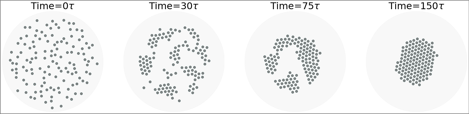
Figure 4: Flow-induced phase separation of active particles at a plane no-slip wall. Starting from a non-crystalline distribution, active particles crystallize into a single cluster due to long-ranged active hydrodynamic interactions between them (Singh and Adhikari, 2016).

Denoting the $x$-component of the active hydrodynamic drag as $F_{x}^{\mathcal{A}}$ and using the leading form for $\gamma_{21}^{xz}$ we have

$$F_{x}^{\mathcal{A}}=\gamma_{21}^{xz}v_{s}=\gamma_{{\scriptscriptstyle\parallel}}\gamma_{\perp}G_{xz}^{\text{w}}v_{s}=-\frac{\gamma_{{\scriptscriptstyle\parallel}}\gamma_{\perp}v_{s}}{2\pi\eta}\frac{3h^{3}}{(r^{2}+4\bar{h}^{2})^{5/2}}r^{x},$$ (21)

where $\gamma_{{\scriptscriptstyle\parallel}}$ and $\gamma_{\perp}$ are the self-friction coefficients in the directions parallel ($\parallel$) and perpendicular ($\perp$) to the wall (Kim and Karrila, 1991). This shows that the active drag force can be written as the gradient of a potential

$$\Phi(\boldsymbol{r})=-\frac{\gamma_{{\scriptscriptstyle\parallel}}\gamma_{\perp}v_{s}}{2\pi\eta}\frac{h^{3}}{(r^{2}+4\bar{h}^{2})^{3/2}},$$ (22)

whose strength depends on the propulsion speed. Potentials of identical functional form, but with different prefactors, have been obtained before for electrophoresis (Squires, 2001) and thermophoresis (Di Leonardo et al., 2009) without associating them to an active drag force, as we have done here. In spite of the non-equilibrium origin of the potential, it leads to a Gibbs distribution for the particle positions, $P\sim\exp[-(\Phi+U)/k_{B}T]$, as the Ito equation satisfies potential conditions whenever $\gamma_{12}^{xx}$, and by Onsager symmetry $\gamma_{21}^{xx}$, is a gradient. This understanding of the active Brownian hydrodynamics of a pair of bottom-heavy active particles near a plane wall rationalizes the ubiquitously observed crystallization of active particles near plane boundaries (Theurkauff et al., 2012; Palacci et al., 2013; Buttinoni et al., 2013; Chen et al., 2015; Petroff et al., 2015; Thutupalli et al., 2018; Aubret et al., 2018), which is our next example.

VII Example 4 - Flow-induced phase separation at a wall

Our fourth example demonstrates the flow-induced phase separation (FIPS) of active particles at a plane no-slip wall. We use the same model of active particles as described in the Example 3 but consider a large number of them. As before, the slip is truncated to contain only $1s$ and $3t$ modes of vectorial symmetry, which are parametrized in term of the orientation $\boldsymbol{p}_{i}$ of the colloids, see Eqs.(13) and (14). All colloids are oriented along the normal to the wall, such that $\boldsymbol{p}_{i}=-\hat{\boldsymbol{z}}$. In experiment, the active force $\sim 6\pi\eta bv_{s}$, is of the order $10^{-13}$N in (Jiang et al., 2010; Palacci et al., 2013), while $10^{-11}$N in (Petroff et al., 2015). Thus, it is orders of magnitude larger than the Brownian force $k_{B}T/b\sim 10^{-15}$N, which we ignore for this example.

The code and snapshots from the simulations are shown in Fig.(4). The initial random distribution of positions is provided by $\mathtt{pystokes.utils.initialConditionRandom(Np)}$. The rigid body motion class is instantiated as $\mathtt{pystokes.wallBounded.Rbm}$, while the Lennard-Jones inter-particle and particle-wall forces are obtained from classes $\mathtt{pystokes.forceFields.Forces}$. A short function computes the velocity that is passed to a standard Python integrator which advances the system in time and saves positional data. This is used to plot the snapshots at specified time instants.

VIII Example 5 - Irreducible autophoretic fields

⬇

# ex5.py: chemical field of an autphoretic colloid - unbounded domain (first row) and near a wall (second)

import pystokes, numpy as np, matplotlib.pyplot as plt

# particle radius, fluid viscosity, and number of particles

b, D, Np = 1.0, 1.0/6.0, 1

#initialise

r, p = np.array([0.0, 0.0, 5]), np.array([0.0, 0.0, 1])

# irreducible coeffcients

J0 = np.ones(Np);

J1 = pystokes.utils.irreducibleTensors(1, p)

J2 = pystokes.utils.irreducibleTensors(2, p)

# space dimension , extent , discretization

dim, L, Ng = 3, 10, 64;

# instantiate the phoretic field class class

ufield = pystokes.phoreticUnbounded.Field(radius=b, particles=Np, phoreticConstant=D, gridpoints=Ng*Ng)

wfield = pystokes.phoreticWallBounded.Field(radius=b, particles=Np, phoreticConstant=D, gridpoints=Ng*Ng)

# plot using subplots on a given grid

rr, vv = pystokes.utils.gridYZ(dim, L, Ng)

plt.figure(figsize=(24, 8), edgecolor=’gray’, linewidth=4)

plt.subplot(231); vv=vv*0; ufield.phoreticField0(vv, rr, r, J0)

pystokes.utils.plotContoursYZ(vv, rr, r,offset=1e-8, title=’m=0’)

plt.subplot(232); vv=vv*0; ufield.phoreticField1(vv, rr, r, J1)

pystokes.utils.plotContoursYZ(vv, rr, r, offset=1e-1,title=’m=1’)

plt.subplot(233); vv=vv*0; ufield.phoreticField2(vv, rr, r, J2)

pystokes.utils.plotContoursYZ(vv, rr, r,offset=1e2, title=’Jm=2’)

plt.subplot(234); vv=vv*0; wfield.phoreticField0(vv, rr, r, J0)

pystokes.utils.plotContoursYZsurf(vv, rr, r, offset=1e-8,)

plt.subplot(235); vv=vv*0; wfield.phoreticField1(vv, rr, r, J1)

pystokes.utils.plotContoursYZsurf(vv, rr, r, offset=1e-2)

plt.subplot(236); vv=vv*0; wfield.phoreticField2(vv, rr, r, J2)

pystokes.utils.plotContoursYZsurf(vv, rr, r, offset=1e+2)

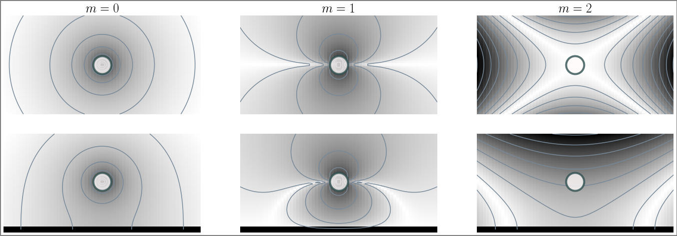
Figure 5: Irreducible phoretic fields: Pseudocolor and contour plot of the phoretic field. The top is the concentration in unbounded domain, while bottom is near a plane wall. The first panel is the concentration due to $m=0$ mode of the flux, while second is for $m=1$, abd third is for $m=2$. The symmetry of the profile follows that of the mode in an unbounded domain. This symmetry is broken in $z-$direction by the introduction of the plane wall.

Our fifth example introduces phoretic fields and, as in Example 1, shows how to plot the irreducible parts of an active phoretic field around a spherical particle. We take the reader step by step from the governing PDE to the expression for the irreducible phoretic fields that the library evaluates and plots. The notation for the particle size, location and orientation are identical to Example 1. We encourage the reader to note the similarities and differences between the two examples.

1. Elliptic PDE. The phoretic field $c\,(\boldsymbol{r})$ satisfies the Laplace equation in the region $V$ exterior to a sphere and satisfies the flux boundary condition on $S$

   $$\lim_{\boldsymbol{r}\rightarrow S}\hat{\boldsymbol{\rho}}\cdot(D\boldsymbol{\nabla}c)=-j^{\mathcal{A}}(\boldsymbol{\rho}),$$ (23)

   where $j^{\mathcal{A}}(\boldsymbol{\rho})$ is the active flux and $D$ is the diffusivity. The fundamental solution of the Laplace equation is by

   $$\nabla^{2}H=-\delta\left(\boldsymbol{r}-\boldsymbol{r^{\prime}}\right)/D,$$ (24)

   where $H$ is the Green’s function which may need to satisfy additional boundary conditions. The normal derivative of the Green’s function is $L=D\hat{\rho}_{\alpha}\nabla_{\alpha}H$.

2. Boundary integral. The fundamental solution, together with Green’s identities, gives the boundary integral representation

   $$c\,(\boldsymbol{r})=\int H(\boldsymbol{r},\,\boldsymbol{R}+\mathbf{\boldsymbol{\rho}})\,j^{\mathcal{A}}(\boldsymbol{\rho})\,\text{d}S+\int L(\boldsymbol{r},\,\boldsymbol{R}+\mathbf{\boldsymbol{\rho}})\,c(\boldsymbol{\rho})\,\text{d}S,$$ (25)

   which expresses the phoretic field in $V$ in terms of a “single-layer” integral involving active flux and a “double-layer” integral involving the boundary phoretic field. The former is specified by the boundary condition; the latter must be determined in terms of it.

3. Spectral expansion. The analytical evaluation of the two integrals is possible if the phoretic field and the flux are expanded spectrally in terms of tensorial spherical harmonics,

   $$c(\boldsymbol{\rho})=\sum_{m=0}^{\infty}w_{m}\mathbf{C}^{(m)}\cdot\mathbf{Y}^{(m)}(\bm{\hat{\rho}}),\qquad j^{\mathcal{A}}(\boldsymbol{\rho})=\sum_{m=0}^{\infty}\tilde{w}_{m}\mathbf{J}^{(m)}\cdot\mathbf{Y}^{(m)}(\bm{\hat{\rho}}),$$ (26)

   where $\mathbf{C}^{(m)}$ and $\mathbf{J}^{(m)}$ are $l$-th rank tensorial coefficients, symmetric and irreducible in all their indices. The orthogonality of the tensorial harmonics implies that

   $$\mathbf{C}^{(m)}=\tilde{w}_{m}\int c(\boldsymbol{R}+\bm{\rho})\mathbf{Y}^{(m)}(\bm{\hat{\rho}})d\text{S},\qquad\mathbf{J}^{(m)}=w_{m}\int j(\boldsymbol{R}+\bm{\rho})\mathbf{Y}^{(m)}(\bm{\hat{\rho}})d\text{S}.$$ (27)

4. Ritz-Galerkin discretization. Letting the point $\boldsymbol{r}$ approach $S$ from $V$ and requiring the phoretic field to attain its value on the boundary leads to an integral equation for it. Multiplying both sides of the integral equation by the $l$-th harmonic and integrating yields an infinite-dimensional system of linear equations for the coefficients of the phoretic field,

   $$\tfrac{1}{2}\mathbf{C}^{(l)}=\boldsymbol{H}^{(l,l^{\prime})}\cdot\mathbf{J}^{(l^{\prime})}+\boldsymbol{L}^{(l,l^{\prime})}\cdot\mathbf{C}^{(l^{\prime})},$$ (28)

   where the matrix elements $\boldsymbol{H}^{(l,\,l^{\prime})}$ and $\boldsymbol{L}^{(l,\,l^{\prime})}$ are give in terms of the Green’s function and its normal derivative. These can be evaluated analytically (R. Singh et al., 2019).

5. Truncation: The infinite-dimensional linear system has to be truncated to a finite-dimensional linear system for tractability. We truncate the system at $l=2$, so that the phoretic field and its flux are

   $$c(\bm{\rho})=C^{(0)}+\mathbf{C}^{(1)}\cdot\mathbf{Y}^{(1)}+\tfrac{1}{6}\mathbf{C}^{(2)}\cdot\mathbf{Y}^{(2)},\qquad 4\pi b^{2}\,j^{\mathcal{A}}(\bm{\rho})=J^{(0)}+3\mathbf{J}^{(1)}\cdot\mathbf{Y}^{(1)}+5\mathbf{J}^{(2)}\cdot\mathbf{Y}^{(2)}.$$ (29)

   The solution of the finite-dimensional linear system yields a linear relation between the coefficients of the field and its flux, the “elastance relations”, $\mathbf{C}^{(m)}=-\boldsymbol{\varepsilon}^{(m,m^{\prime})}\cdot\mathbf{J}^{(m^{\prime})}$. In an unbounded domain, the elastance tensors $\boldsymbol{\varepsilon}^{(m,m^{\prime})}$ take on a particularly simple form: they are diagonal in the $m$ indices, $\boldsymbol{\varepsilon}^{(m,m^{\prime})}\equiv\delta_{mm^{\prime}}\Delta^{(m)}/4\pi Dw_{m}$ so that the single scalar $4\pi Dw_{m}$ determines them. For $m=0$ this is the familiar coefficient $1/4\pi b$ for the inverse capacitance of a spherical conductor.

Inserting the truncated spectral expansions for the phoretic field and the active flux, eliminating the unknown phoretic coefficients for the known flux coefficients, expanding the Green’s function about the center of the sphere and finally using orthogonality of the tensorial harmonics, we obtain the phoretic field due to each irreducible flux mode as

$$c^{0}(\boldsymbol{r})=HJ^{(0)},\qquad c^{1}(\boldsymbol{r})=(\boldsymbol{\nabla}H)\cdot\mathbf{J}^{(1)},\qquad c^{2}(\boldsymbol{r})=\tfrac{4}{3}(\boldsymbol{\nabla}\boldsymbol{\nabla}H)\cdot\mathbf{J}^{(2)},$$ (30)

We emphasise that these expressions are valid for any Green’s function of the Laplace equation, provided they satisfy the additional boundary conditions that may be imposed. For this example we consider the Green’s function in an unbounded domain, where the flux vanishes at infinity,

$$H_{\alpha\beta}^{\text{o}}(\boldsymbol{r}-\boldsymbol{r}^{\prime})=\frac{1}{8\pi D}\nabla^{2}|\boldsymbol{r}-\boldsymbol{r}^{\prime}|.$$ (31)

and in a domain confined by an infinite planar wall at which the flux vanishes,

$$H_{\alpha\beta}^{\text{w}}(\boldsymbol{r},\boldsymbol{r}^{\prime})=H_{\alpha\beta}^{\text{o}}(\boldsymbol{r}-\boldsymbol{r}^{\prime})+H_{\alpha\beta}^{\text{o}}(\boldsymbol{r}-\boldsymbol{r}^{*\prime}).$$ (32)

Here, as earlier, $\boldsymbol{r}^{*\prime}=\boldsymbol{\mathcal{M}}\cdot\boldsymbol{r}^{\prime}$ is the mirror image of the point, where $\boldsymbol{\mathcal{M}}=\boldsymbol{I}-2\mathbf{\hat{z}}\mathbf{\hat{z}}$ is the reflection operator.

The code listed in Fig.(5) computes the irreducible concentration profile for $m=0$,1,2 modes of the active flux for radius $b=1$, diffusion constant $D=1$, location $\boldsymbol{R}=(0,0,5)$ and orientation $\boldsymbol{p}=(0,0,1).$ The coefficients are parametrised as $J^{(0)}=1$, $J_{\alpha}^{(1)}=p_{\alpha}$ and $J_{\alpha\beta}^{(2)}=p_{\alpha}p_{\alpha}-\delta_{\alpha\beta}/3$. These are supplied to the $\mathtt{ufield}$ class which is instantiated for an unbounded domain. The $m$-th irreducible component of the field is computed by the calling the function $\mathtt{ufield.phoreticFieldm}$. This is passed to a generic plotting function to compute the pseudocolor plot in a plane of symmetry. These are shown in the code output where the spherical , polar, and nematic symmetries of the $m=0$, 1 and $2$ modes can be seen. The second row shows the same fields near a plane wall, obtained by changing the flow instantiation to $\mathtt{wfield}$ class. The fields have reduced symmetry in $z-$direction due to the introduction of the plane wall.

IX Example 6 - Autophoretic arrest of flow-induced phase separation

⬇

# ex6.py: Arrested clustering of autphoretic colloids near a wall

import pystokes, numpy as np, matplotlib.pyplot as plt

# particle radius, self-propulsion speed, number and fluid viscosity

b, vs, Np, eta = 1.0, 1.0, 256, 0.1

#initialise

r = pystokes.utils.initialCondition(Np) # initial random distribution of positions

p = np.zeros(3*Np); p[2*Np:3*Np] = -1 # initial orientation of the colloids

rbm = pystokes.wallBounded.Rbm(radius=b, particles=Np, viscosity=eta)

phoresis = pystokes.phoreticWallBounded.Phoresis(radius=b, particles=Np, phoreticConstant=eta)

forces = pystokes.forceFields.Forces(particles=Np)

N1, N2 = 3*Np, 6*Np # define two constants for convenience

def rhs(rp):

"""

* right hand side of the rigid body motion equations

* rp: is the array of position (r) and orientations (p) of the colloids

* returns \dot{rp} so that rp can be updated using an integrator

"""

#initialise the positions and orientation, forces at each time step

r = rp[0:N1]; p = rp[N1:N2];

F,v,o,C1 = np.zeros(N1),np.zeros(N1),np.zeros(N1),np.zeros(N1)

# rbm contributions from body forces

forces.lennardJonesWall(F, r, lje=0.012, ljr=5, wlje=1.2, wljr=3.4)

rbm.mobilityTT(v, r, F)

#phoretic field on the surface of colloids

J0, J1 = .4*np.ones(Np), pystokes.utils.irreducibleTensors(1, p)

phoresis.elastance10(C1, r, J0); phoresis.elastance11(C1, r, J1)

# active contributions to the rbm

M0=1; V1s=-pystokes.utils.couplingTensors(0, p, M0)*C1; V3t=0.6*V1s

rbm.propulsionT3t(v, r, V3t); v += V1s

return np.concatenate( (v,o) )

# simulate the resulting system and plot at specific time instants

Tf, Npts = 300, 256

pystokes.utils.simulate(np.concatenate((r,p)), Tf,Npts,rhs,integrator=’odeint’, filename=’arrestedClusters’)

pystokes.utils.plotConfigs(t=[1, 100, 200, 256], ms=60, tau=(Tf/Npts)/(b/vs), filename=’arrestedClusters’)

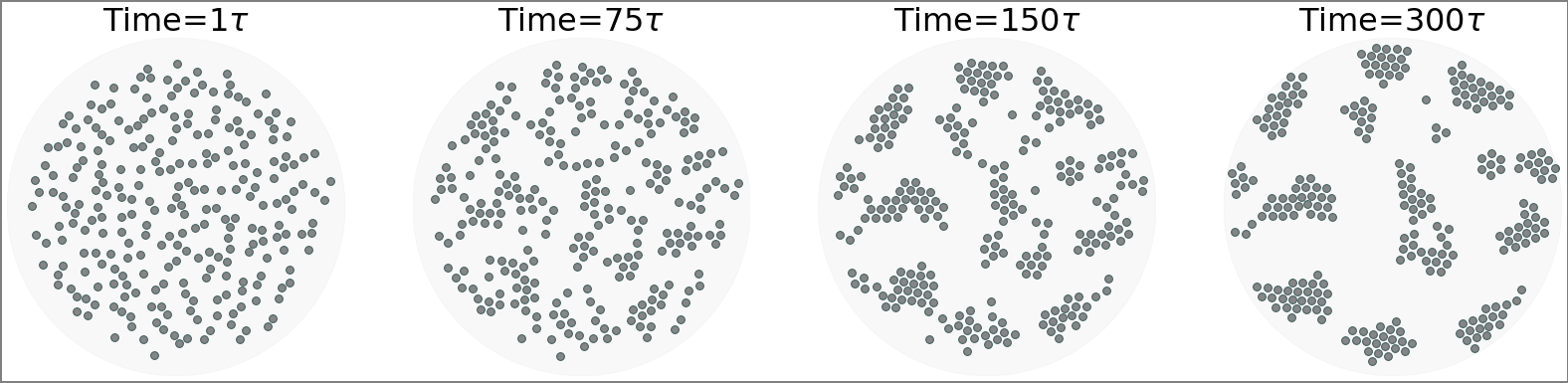
Figure 6: Phoretic arrest of flow-induced phase separation. In this example, we extend the results of Fig.(4) by adding phoretic interactions. We show that this can lead to arrest of flow-induced phase separation when the phoretic interactions between the colloids are repulsive. The length scale at which the clusters are arrested is proportional the self-propulsion speed of an isolated colloid (R. Singh et al., 2019), in excellent agreement with experimental observations (Theurkauff et al., 2012; Buttinoni et al., 2013).

Our sixth example describes the modification of active slip by phoretic interactions between active particles and the resulting arrest of flow-induced phase separation seen in Example 4. The slip, from being an apriori specified quantity for each particle, must now be computed from the interacting phoretic fields of all particles. In the previous example, we obtained the phoretic field for a specified surface flux. Here we show how to coupled it to the Stokes equation and obtain both the hydrodynamic and phoretic interactions of active colloids. The coupling of the Stokes and Laplace equation and Laplace equations is through the following expression for the active slip (Anderson, 1989),

$$\boldsymbol{v}^{\mathcal{A}}(\boldsymbol{\rho}_{i}) =\mu_{c}(\boldsymbol{\rho}_{i})\boldsymbol{\nabla}_{s}\,c(\boldsymbol{\rho}_{i}).$$ (33)

In the previous section, we showed that $\mathbf{C}_{i}^{(m)}=-\boldsymbol{\varepsilon}{}_{ik}^{(m,m^{\prime})}\cdot\mathbf{J}_{k}^{(m^{\prime})}.$ This solution can be used to obtain the coefficients of the slip as $\mathbf{V}_{i}^{(l)}=-\boldsymbol{\chi}^{(l,m)}\cdot\mathbf{C}_{i}^{(m)},$ where $\boldsymbol{\chi}^{(l,m)}$ is a coupling tensor of rank $(l+m)$ that depends on the phoretic mobility $\mu_{c}$ (R. Singh et al., 2019). Thus the problem is fully specified once the coefficients of the flux and phoretic mobility on the surface of all the particles is given.

For this example, we consider an active surface flux $j^{\mathcal{A}}$ with spherical and polar modes and a phoretic mobility that is constant,

$$4\pi b^{2}\,j^{\mathcal{A}}(\boldsymbol{\rho}_{i})=J^{(0)}+3\,J^{(1)}\boldsymbol{p}_{i}\cdot\boldsymbol{\hat{\rho}}_{i},\qquad 4\pi b^{2}\,\mu_{c}(\boldsymbol{\rho}_{i})=M^{(0)}.$$ (34)

Phoretic interactions are computed with he no-flux condition at the plane wall using the Green’s function of Eq.(32). Hydrodynamic interactions are computed with the no-slip on the plane wall using the Lorentz-Blake tensor of Eq.(10).

The code and snapshots from the simulations are shown in Fig.(6). The $\mathtt{pystokes.phoreticWallBounded.Phoresis}$ class is used to compute the active slip which is fed into $\mathtt{pystokes.wallBounded.Rbm}$ to compute the rigid body motion. As before, a short function is used to compute the velocity that is passed on to a standard Python integrator which advances the system in time and saves position data. This is used to plot the snapshots at specified time instants.

⬇

# ex7.py: Benchmarks

import numpy as np, matplotlib.pyplot as plt, pystokes, time, matplotlib as mpl

#computes time taken to simulate Np particles

def timeTaken(Np):

b, vs, eta = 1.0, 1.0, 0.1; r = 2*np.linspace(-3*Np, 3*Np, 3*Np)

p, v = np.ones(3*Np), np.zeros(3*Np)

RBM = pystokes.wallBounded.Rbm(radius=b, particles=Np, viscosity=eta)

V3t = p; t1 = time.perf_counter(); RBM.propulsionT3t(v, r, p)

return time.perf_counter() - t1

xP = np.arange(2000, 21000, 2000)

tP1 = np.zeros(np.size(xP))

for i in range(np.size(xP)):

tP1[i]=timeTaken(xP[i])

plt.figure(figsize=(16, 14))

mpl.rc(’hatch’, color=’k’, linewidth=22.5)

mss=24; plt.xticks(fontsize=mss); plt.yticks(fontsize=mss)

plt.semilogy(xP, tP1, ’-*’, ms=mss+3, label="1 Core", lw=3, color=’lightslategray’, mfc=’w’, mew=2, alpha=1)

plt.legend(fontsize=mss, loc=4)

plt.xlabel(’# colloids (thousands)’, fontsize=mss+5)

plt.ylabel(’CPU time (secs)’, fontsize=mss+5)

plt.grid()

# repeat for different number of cores. We plot a precompiled set of benchmarks

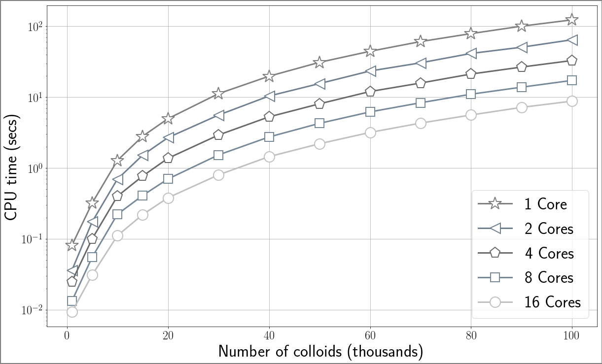
Figure 7: Benchmarks for computing the rigid body motion due to $\mathbf{V}^{(3t)}$ slip mode in the unbounded geometry of Stokes flow, on a 16-core machine, using PyStokes. The present implementation shows a linear scaling with the number of CPU cores, and quadratic scaling with number of particles, when the matrix-vector products are computed as direct sums.

X Code performance

Our final example is on performance and benchmarks. We show that our codes scales linearly with the number of CPU cores and quadratically with $N$, the number of particles simulated. In the current implementation, the velocities of about $10^{5}$ particles can be computed in a few seconds for a mode of the active slip, as shown in Fig.(7). With current many-core architectures a dynamic simulation of about $N\sim 10^{5}$ is within reach. For larger number of particles, accelerated summation methods are desirable, which can reduce the cost to $\mathcal{O}(N\log N)$ (Barnes and Hut, 1986; Sierou and Brady, 2001) or even $\mathcal{O}(N)$ (Greengard and Rokhlin, 1987; Sangani and Mo, 1996; Ladd, 1994). These methods can be implemented in the present numerical architecture as an improvement over the direct kernel sum, while maintaining the overall library structure.

XI What else ?

In the six examples above we demonstrated the use of PyStokes library for simulating hydrodynamic and phoretic phenomena. These do not exhaust the capabilities of the library and much else can be done with them. We conclude by listing implemented, implementable and unimplementable features. Implemented but not shown: the library supports periodic geometries (Singh, 2018) and parallel plane walls (Thutupalli et al., 2018; Sarkar et al., 2018). Polymers (Laskar and Adhikari, 2015), membranes and other hierarchical assemblies of active particles can be simulated. Can be implemented: other boundary conditions, for instance flows interior to a spherical domain such as a liquid drop, near-field lubrication interactions, and numerical solutions of the linear system can be implemented in the current design, with treecode or fast-multipole accelerations. Cannot be implemented: irregular geometries for which analytical forms of the Green’s functions of the Laplace and Stokes equations cannot be evaluated analytically and/or irregularly shaped particles on whose boundaries globally defined spectral basis functions are not available. A shorter version of this paper has been published in JOSS (Singh and Adhikari, 2020).

References

- Brennen and Winet (1977) C. Brennen and H. Winet, Annu. Rev. Fluid Mech. 9, 339 (1977).
- Ebbens and Howse (2010) S. J. Ebbens and J. R. Howse, Soft Matter 6, 726 (2010).
- Anderson (1989) J. L. Anderson, Annu. Rev. Fluid Mech. 21, 61 (1989).
- Zhang et al. (2017) J. Zhang, E. Luijten, B. A. Grzybowski, and S. Granick, Chem. Soc. Rev. 46, 5551 (2017).
- Singh et al. (2015) R. Singh, S. Ghose, and R. Adhikari, J. Stat. Mech 2015, P06017 (2015).
- Singh and Adhikari (2018) R. Singh and R. Adhikari, J. Phys. Commun. 2, 025025 (2018).
- R. Singh et al. (2019) R. Singh, R. Adhikari, and M. E. Cates, J. Chem. Phys. 151, 044901 (2019).
- Weideman and Reddy (2000) J. A. Weideman and S. C. Reddy, ACM Trans. Math. Software 26, 465 (2000).
- Higham (2001) D. J. Higham, SIAM review 43, 525 (2001).
- Trefethen (2000) L. N. Trefethen, Spectral methods in MATLAB, Vol. 10 (SIAM, Philadelphia, 2000).
- Theurkauff et al. (2012) I. Theurkauff, C. Cottin-Bizonne, J. Palacci, C. Ybert, and L. Bocquet, Phys. Rev. Lett. 108, 268303 (2012).
- Palacci et al. (2013) J. Palacci, S. Sacanna, A. P. Steinberg, D. J. Pine, and P. M. Chaikin, Science 339, 936 (2013).
- Buttinoni et al. (2013) I. Buttinoni, J. Bialké, F. Kümmel, H. Löwen, C. Bechinger, and T. Speck, Phys. Rev. Lett. 110, 238301 (2013).
- Chen et al. (2015) X. Chen, X. Yang, M. Yang, and H. P. Zhang, EPL 111, 54002 (2015).
- Petroff et al. (2015) A. P. Petroff, X.-L. Wu, and A. Libchaber, Phys. Rev. Lett. 114, 158102 (2015).
- Thutupalli et al. (2018) S. Thutupalli, D. Geyer, R. Singh, R. Adhikari, and H. A. Stone, Proc. Natl. Acad. Sci. 115, 5403 (2018).
- Aubret et al. (2018) A. Aubret, M. Youssef, S. Sacanna, and J. Palacci, Nat. Phys 14, 1114 (2018).
- Odqvist (1930) F. K. G. Odqvist, Mathematische Zeitschrift 32, 329 (1930).
- Ladyzhenskaia (1969) O. A. Ladyzhenskaia, The mathematical theory of viscous incompressible flow, Mathematics and its applications (Gordon and Breach, 1969).
- Youngren and Acrivos (1975) G. Youngren and A. Acrivos, J. Fluid Mech. 69, 377 (1975).
- Zick and Homsy (1982) A. A. Zick and G. M. Homsy, J. Fluid Mech. 115, 13 (1982).
- Pozrikidis (1992) C. Pozrikidis, Boundary Integral and Singularity Methods for Linearized Viscous Flow (Cambridge University Press, 1992).
- Muldowney and Higdon (1995) G. P. Muldowney and J. J. L. Higdon, J. Fluid Mech. 298, 167 (1995).
- Cheng and Cheng (2005) A. H.-D. Cheng and D. T. Cheng, Eng. Anal. Bound. Elem. 29, 268 (2005).
- Jackson (1962) J. D. Jackson, Classical electrodynamics (Wiley, 1962).
- Lorentz (1896) H. A. Lorentz, Versl. Konigl. Akad. Wetensch. Amst 5, 168 (1896).
- Hess (2015) S. Hess, Tensors for physics (Springer, 2015).
- Boyd (2000) J. P. Boyd, Chebyshev and Fourier spectral methods (Dover, 2000).
- Finlayson and Scriven (1966) B. A. Finlayson and L. E. Scriven, Appl. Mech. Rev 19, 735 (1966).
- Saad (2003) Y. Saad, Iterative methods for sparse linear systems (SIAM, 2003).
- Ghose and Adhikari (2014) S. Ghose and R. Adhikari, Phys. Rev. Lett. 112, 118102 (2014).
- Singh and Adhikari (2016) R. Singh and R. Adhikari, Phys. Rev. Lett. 117, 228002 (2016).
- Batchelor (2000) G. K. Batchelor, An introduction to fluid dynamics (Cambridge university press, 2000).
- Goldstein (2015) R. E. Goldstein, Ann. Rev. Fluid Mech. 47, 343 (2015).
- Singh and Adhikari (2017) R. Singh and R. Adhikari, Eur. J. Comp. Mech 26, 78 (2017).
- Weeks et al. (1971) J. D. Weeks, D. Chandler, and H. C. Andersen, J. Chem. Phys. 54, 5237 (1971).
- Kim and Karrila (1991) S. Kim and S. J. Karrila, Microhydrodynamics: Principles and Selected Applications (Butterworth-Heinemann, Boston, 1991).
- Squires (2001) T. M. Squires, J. Fluid Mech. 443, 403 (2001).
- Di Leonardo et al. (2009) R. Di Leonardo, F. Ianni, and G. Ruocco, Langmuir 25, 4247 (2009).
- Jiang et al. (2010) H.-R. Jiang, N. Yoshinaga, and M. Sano, Phys. Rev. Lett. 105, 268302 (2010).
- Barnes and Hut (1986) J. Barnes and P. Hut, Nature 324, 446 (1986).
- Sierou and Brady (2001) A. Sierou and J. F. Brady, J. Fluid Mech. 448, 115 (2001).
- Greengard and Rokhlin (1987) L. Greengard and V. Rokhlin, J. Comp. Phys. 73, 325 (1987).
- Sangani and Mo (1996) A. S. Sangani and G. Mo, Phys. Fluids 8, 1990 (1996).
- Ladd (1994) A. J. C. Ladd, J. Fluid Mech. 271, 285 (1994).
- Singh (2018) R. Singh, Microhydrodynamics of active colloids [HBNI Th131], Ph.D. thesis, HBNI (2018).
- Sarkar et al. (2018) D. Sarkar, R. Singh, A. Som, C. K. Manju, M. A. Ganayee, R. Adhikari, and T. Pradeep, J. Phys. Chem. C 122, 17777 (2018).
- Laskar and Adhikari (2015) A. Laskar and R. Adhikari, Soft matter 11, 9073 (2015).
- Singh and Adhikari (2020) R. Singh and R. Adhikari, J. Open Source Software 5, 2318 (2020).
- sto (2019) “Stokes 200 symposium,” https://www.pem.cam.ac.uk/alumni-development/events/stokes-200-symposium (2019).