Continuous Aharonov–Bohm effect

Abstract

The Aharonov–Bohm effect in a model system described by the generalized Schrödinger equation is considered. The scattering cross section is calculated in the standard formulation: an electron beam impinges on a long impenetrable solenoid encompassing a magnetic field. It is shown that the incident wave is scattered regardless of whether the magnetic flux through the solenoid is an integer of flux quanta whereby the scattering cross section becomes a continuously nonzero function of the total magnetic flux. The problem may find its application in investigations of the soliton-magnon interaction in the low-dimensional magnetism.

Key words: Aharonov–Bohm effect, Schrödinger equation, scattering theory

PACS: 03.65-w, 03.65.Nk, 03.65.Vf

Abstract

Ðîçãëÿíóòî åôåêò Ààðîíîâà-Áîìà â ìîäåëüíié ñèñòåìi, ùî îïèñóєòüñÿ óçàãàëüíåíèì ðiâíÿííÿì Øðåäiíãåðà. Îáчèñëåíî ïåðåðiç ðîçñiÿííÿ â ñòàíäàðòíîìó ôîðìóëþâàííi: ïóчîê åëåêòðîíiâ ïàäàє íà äîâãèé íåïðîíèêíèé ñîëåíî¿ä ç ìàãíiòíèì ïîëåì. Ïîêàçàíî, ùî ïàäàþчà õâèëÿ ðîçñiþєòüñÿ íåçàëåæíî âiä òîãî чè є ïîòiê чåðåç ñîëåíî¿ä öiëèì чèñëîì êâàíòiâ ïîòîêó, âíàñëiäîê чîãî ïåðåðiç ðîçñiÿííÿ ñòàє íåïåðåðâíî íåíóëüîâîþ ôóíêöiєþ ïîâíîãî ìàãíiòíîãî ïîòîêó. Öÿ ïðîáëåìà ìîæå çíàéòè ñâîє çàñòîñóâàííÿ ó äîñëiäæåííi ñîëiòîí-ìàãíîííî¿ âçàєìîäi¿ â íèçüêîðîçìiðíîìó ìàãíåòèçìi.

Ключовi слова: åôåêò Ààðîíîâà-Áîìà, ðiâíÿííÿ Øðåäiíãåðà, òåîðiÿ ðîçñiÿííÿ

1 Introduction

The Aharonov–Bohm effect demonstrates the significance of the vector potential, $\mathbf{A}$, in the quantum theory. It was first described by Aharonov and Bohm in their original work [1] in 1959 and was intensively studied afterwards by a number of authors [4, 5, 2, 3, 6, 7]. The effect refers to the interference phenomena of charged particles (electrons) traveling around an extremely long isolated solenoid whose radius tends to zero. The solenoid is a source of a magnetic field, $\mathbf{B}=\textrm{rot}~{}\mathbf{A}$. The magnetic flux density is concentrated in the small region inside the solenoid, so the total flux is $\Phi_{\textrm{s}}=\int\mathbf{B}\textrm{d}\mathbf{s}=\oint\mathbf{A}\textrm{d}\mathbf{l}$, where integration can be made through every closed circuit encircling the singularity. The movement of the particles takes place outside the magnetic field region, where $\mathbf{B}=0$. Nevertheless, the vector potential does have a physical effect on their scattering. In the simplest case, when an electron moves on a closed trajectory including the solenoid, the phase of the electron wave function is additionally changed by $-2\piup\alpha=2\piup\Phi_{\textrm{s}}/\Phi_{0}$, where $\Phi_{0}$ is the flux quantum. The requirement for the wave function to be single-valued leads to the quantization of the flux by $\Phi_{0}$. The value of $\alpha$ is determined by a number of flux quanta in the total flux through the solenoid and depends only on the topological invariant $\oint\mathbf{A}\textrm{d}\mathbf{l}$. Within the problem of the interference of two coherent electron beams bypassing the solenoid from different sides, the vector potential manifests itself as an additional shift of the interference picture. When the flux inside the solenoid is a multiple of flux quanta, $\alpha$ is an integer and the interference is constructive (the relative phase shift depends only on the difference between the paths traveled). Noninteger $\alpha$ means that the electron wave function acquires an additional phase factor and the interference pattern shifts. In fact, the solenoid plays a role of an impenetrable flux line that makes the field-free region of space multiply connected. The interaction of particles with the topological peculiarity produces an additional phase shift in their wave function. It can be experimentally detected by measuring the arrangement and the sharpness of the interference bands.

Nowadays, the relevance of the problem is maintained by the development of nanoelectronic, mesoscopic and spintronic devices, and quantum computers. The Aharonov–Bohm effect found its application in single-electron transistors with suspended nanotubes [8, 9]. Electrons passing through the device interfere on the nanotubes vibrating in the presence of a magnetic field [10]. The Aharonov–Bohm effect is often involved in comprehending different phenomena in the quantum physics. The existence of an analogous effect was discussed in the physics of low-dimensional magnetism: in the problems of vortex-magnon scattering in easy-plane ferromagnets [11, 12] and skyrmion-magnon scattering [13, 14], including skyrmions in chiral magnets [14]. The non-trivial topology of an isolated soliton gives rise to terms in the magnon dynamical equations similar to the term with vector potential $\mathbf{A}$ in the Schrödinger equation. In cone state ferromagnets, this Aharonov–Bohm type of interaction with the nonlinear vortex core causes a significant doublet splitting of magnon modes [15, 16]. In chiral magnets, there appears a skew and rainbow scattering of magnons, characterized by an asymmetric differential cross section [17, 18]. However, equations describing magnon dynamics can be much more complicated than the standard Schrödinger equation. For this reason, various generalizations of the Aharonov–Bohm effect are of great interest.

In this paper, we investigate the existence of the Aharonov–Bohm effect in a model system that is described by the generalized Schrödinger equation. It appears in the study of quantum many-particle systems by means of the approximating Hamiltonian method originally developed by N.N. Bogolyubov. The method is equivalent to introducing some quasiparticles that are capable of condensing into a single quantum state [19, 20]. In the effective Hamiltonian, this leads to the appearance of anomalous average terms describing the exchange of particles between condensate and noncondensate states. The model approach allows one to turn to the exactly solvable quantum models that cannot be obtained by means of the perturbation theory and, therefore, occupies an important place in condensed matter physics [21]. However, the Aharonov–Bohm problem in such systems, to the best of our knowledge, has not been considered yet.

In the present work, we obtain an asymptotic solution of the generalized Schrödinger equation in presence of the vector potential (section 2) and solve a direct scattering problem (section 3). We numerically calculate the scattering cross section and show that the scattering picture is qualitatively different from the one of the original Aharonov–Bohm problem (section 4). We also briefly discuss possible applications of the model problem in section 5.

2 Solution of the generalized Schrödinger equation in the presence of a magnetic flux line

The generalized Schrödinger equation may be derived as the Euler equation of some variational problem [21], in which the Lagrangian density has the form

$$L=\mathrm{i}\hbar\psi^{*}\frac{\partial\psi}{\partial t}-\psi^{*}\frac{1}{2m_{0}}\left(-\mathrm{i}\hbar\nabla-\frac{e}{c}\mathbf{A}\right)^{2}\psi-\psi^{*}a\psi-\frac{b}{2}(\psi^{*}\psi^{*}+\psi\psi).$$ (2.1)

For convenience, we use the original formulation of the Aharonov–Bohm problem as a concrete example that allows one to rely on the formulae obtained in the work [1] without changing them. Additionally, we introduce coordinate independent normal and abnormal pairing potentials indicated by $a$ and $b$, respectively. Specific values of these potentials, as well as a possible origin of the Lagrangian density (2.1), are discussed in section 5.

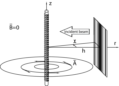
Figure 1: The schematic picture of the system: a coherent electron beam is scattered by an infinitely long impenetrable solenoid. The incident beam is coming from the right where $\chi=0$. Magnetic field outside the solenoid: $\mathbf{B}=0$. Intensity of bands on a screen is determined by the scattering cross section shown in figure 3.

A schematic picture of the system is shown in figure 1. A coherent electron beam is scattered by an infinitely long impenetrable solenoid located along the $z$-axis of the cylindrical geometry. Its radius tends to zero, while the total flux, $\Phi_{\textrm{s}}$, remains fixed. The vector potential of the solenoid is $\mathbf{A}=\Phi_{\textrm{s}}/2\piup r\mathbf{e}_{\chi}$, where $\mathbf{e}_{\chi}$ is the unit azimuthal vector, $r$ and $\chi$ are the radial and azimuthal coordinates, respectively. We also use the traditional notation of the flux quantum $\Phi_{0}=2\pi\hbar c/e$, where $c$ is the speed of light, $e$ is the electron charge, $\hbar$ is the Planck constant. The energy and the wave vector of the electron in the incident wave are denoted as $\omega\hbar$ and $\mathbf{k}$, and $m_{0}$ is the electron mass.

The variation of the Lagrangian $\mathcal{L}=\int L\textrm{d}\textbf{r}$ results in

$$\mathrm{i}\hbar\frac{\partial\psi}{\partial t}=\frac{1}{2m_{0}}\left(-\mathrm{i}\hbar\nabla-\frac{e}{c}\mathbf{A}\right)^{2}\psi+a\psi+b\psi^{*}.$$ (2.2)

The axial symmetry of the problem means that the solution of equation (2.2) does not depend on $z$-coordinate. We separate azimuthal and radial variables by writing the electron wave function as the sum of partial waves

$$\psi=\sum_{m}\left[A_{m}u(r)\exp{(\mathrm{i}m\chi-\mathrm{i}\omega t)}\vphantom{\sum}+B_{m}v(r)\exp(-\mathrm{i}m\chi+\mathrm{i}\omega t)\right].$$ (2.3)

They are marked with azimuthal numbers, $m=0,\pm 1,\pm 2\ldots$, and have amplitudes $A_{m}$ and $B_{m}$. Radial functions $u(r)$ and $v(r)$ depend on $m$ and can be expressed through some cylindrical functions. Thus, for each pair of the radial functions, an eigenvalue problem can be formulated as follows:

$$\begin{Vmatrix}\hat{H}_{+}&b\\ -b&-\hat{H}_{-}\end{Vmatrix}\begin{Vmatrix}u\\ v\end{Vmatrix}=\omega\hbar\begin{Vmatrix}u\\ v\end{Vmatrix},$$ (2.4)

where

$$\hat{H}_{\pm}=-\frac{\hbar^{2}}{2m_{0}}\left[\frac{\textrm{d}^{2}}{\textrm{d}r^{2}}+\frac{\textrm{d}}{r\textrm{d}r}-\frac{(m\pm\alpha)^{2}}{r^{2}}\right]+a.$$ (2.5)

Note that problem (2.4) is invariant under the conjugations $\omega\hbar\rightarrow-\omega\hbar$, $m\rightarrow-m$, and $u\rightarrow v$. Thus, without loss of generality, we can restrict ourselves to a case of the positive energy only, $\omega\hbar>0$.

If there is no magnetic flux $\alpha=0$, then positive and negative energy solutions of eigenvalue problem (2.4) can be easily separated by the Bogolyubov transformation

$$\begin{Vmatrix}\tilde{u}\\ \tilde{v}\end{Vmatrix}=R\begin{Vmatrix}{u}\\ {v}\end{Vmatrix},\;\;R=\begin{Vmatrix}\cos\varepsilon&-\sin\varepsilon\\ \sin\varepsilon&\cos\varepsilon\end{Vmatrix}$$ (2.6)

with the rotation angle

$$\tan 2\varepsilon=\frac{b}{\omega\hbar}.$$ (2.7)

The result can be interpreted as the occurrence of certain quasiparticles [21] with the energy

$$\Lambda=\sqrt{b^{2}+\omega^{2}\hbar^{2}}$$ (2.8)

and a gap spectrum

$$\Lambda=a+\frac{\hbar^{2}k^{2}}{2m_{0}}.$$ (2.9)

In terms of $\omega\hbar$, it is

$$\omega^{2}\hbar^{2}=a^{2}-b^{2}+\frac{\hbar^{2}k^{2}}{m_{0}}a+\frac{\hbar^{4}k^{4}}{4m_{0}^{2}}.$$ (2.10)

In the most general case of a nonzero $\Phi_{\textrm{s}}$, the analysis of eigenvalue problem (2.4) is much complicated by the fact that there are two different equations for $u$ and $v$. The Bogolyubov transformation gives

$$\left(\begin{Vmatrix}\hat{H}_{0}&0\\ 0&-\hat{H}_{0}\end{Vmatrix}+\hat{X}R^{-2}\right)\begin{Vmatrix}\tilde{u}\\ \tilde{v}\end{Vmatrix}=\Lambda\begin{Vmatrix}\tilde{u}\\ \tilde{v}\end{Vmatrix},$$ (2.11)

where

$$\hat{H}_{0}=-\frac{\hbar^{2}}{2m_{0}}\left(\frac{\textrm{d}^{2}}{\textrm{d}r^{2}}+\frac{\textrm{d}}{r\textrm{d}r}-\frac{m^{2}+\alpha^{2}}{r^{2}}\right)+a\,,\;\;\hat{X}=\frac{\hbar^{2}}{2m_{0}}\frac{2m\alpha}{r^{2}}.$$ (2.12)

A new pair of radial eigenfunctions $\tilde{u}$ and $\tilde{v}$ are related due to the potential $\hat{X}$ and can be analyzed only in the sense of their asymptotic behavior. Such an approximation is valid since $\hat{X}$ strongly decreases with the distance. As we are interested only in positive energy solutions ($\Lambda>0$), the function $\tilde{u}$ takes a role of a master function, while $\tilde{v}$ becomes a slave one.

Following the idea of the appearance of quasiparticles, we regard $\tilde{u}(r)$ as the radial part of a new wave function

$$\tilde{\psi}=\sum_{m}c_{m}\tilde{u}(r)\exp\left(\mathrm{i}m\chi-\mathrm{i}\frac{\Lambda}{\hbar}t\right).$$ (2.13)

It describes a particle with energy $\Lambda$ and is the solution of an effective Schrödinger equation

$$\mathrm{i}\hbar\frac{\partial\tilde{\psi}}{\partial t}=\frac{1}{2m_{0}}\left(-\mathrm{i}\hbar\nabla-\frac{e}{c}\tilde{\mathbf{A}}\right)^{2}\tilde{\psi}+V\tilde{\psi}.$$ (2.14)

Here, $\tilde{\mathbf{A}}=\mathbf{{A}}\cos 2\varepsilon=-\tilde{\alpha}\mathbf{e}_{\chi}c\hbar/er$ and

$$V=\frac{\hbar^{2}}{2m_{0}}\frac{\tilde{\alpha}^{2}\tan^{2}2\varepsilon}{r^{2}}+a.$$ (2.15)

The effective potential $V$ has the radially symmetric $r$-dependent part and the constant part $a$. The last one can be considered as an energy level relative to which the quasiparticle energy is measured. Thus, the incident quasiparticles are scattered on the effective barrier $\sim 1/r^{2}$ and the total flux is renormalized as $\tilde{\Phi}_{\textrm{s}}=\Phi_{\textrm{s}}\cos 2\varepsilon$.

The radial function $\tilde{u}(r)$ from the formula (2.13) satisfies the Bessel equation

$$\frac{\hbar^{2}}{2m_{0}}\left(\frac{\textrm{d}^{2}}{\textrm{d}r^{2}}+\frac{\textrm{d}}{r\textrm{d}r}-\frac{\nu^{2}}{r^{2}}\right)\tilde{u}=\Lambda\tilde{u}$$ (2.16)

with the generally noninteger index

$$\nu^{2}=(m+\tilde{\alpha})^{2}+\tilde{\alpha}^{2}\tan^{2}2\varepsilon.$$ (2.17)

On the formulation of the problem, the particles do not penetrate into the region of close vicinity of the solenoid and the probability of finding the particle at the origin approaches zero. For this reason, we restrict a general solution of equation (2.16) to the Bessel function $J_{\nu}(kr)$ of the positive index only, $\nu>0$. The spectrum of the particle is given by expression (2.9).

3 Scattering problem for quasiparticles

Taking into account the results of the previous section, the scattering problem for quasiparticles of the energy $\Lambda$ and impulse $\hbar\mathbf{k}$ can be formulated in a canonical way. A steady beam of particles is scattered by an impenetrable magnetic flux line with the total flux $\tilde{\Phi}_{\textrm{s}}$. The effective potential $V$ created by the flux line is radially symmetric and short ranged. Hence, one can distinguish between incident and scattered waves at large values of $kr$.

The total wave function $\tilde{\psi}$ is given by expression (2.13). The coefficient $c_{m}$ is chosen in a way to present $\tilde{\psi}$ as a superposition of incident plane wave $\tilde{\psi}_{\textrm{inc}}$ and the scattered cylindrical wave,

$$\tilde{\psi}=\tilde{\psi}_{\textrm{inc}}+\mathcal{F}(\chi)\frac{1}{\sqrt{kr}}\exp\left(\mathrm{i}kr-\mathrm{i}\frac{\Lambda}{\hbar}t\right).$$ (3.1)

Scattering function $\mathcal{F}(\chi)$ describes directions of strong and weak scattering of particles. It is fully determined by $\tilde{\alpha}=\alpha\cos 2\varepsilon$ which is exactly the number of flux quanta in the total flux $\tilde{\Phi}_{\textrm{s}}$ taken with the opposite sign. The incident wave is coming from the right, where $\chi=0$,

$$\tilde{\psi}_{\textrm{inc}}=\exp\left(-\mathrm{i}kr\cos\chi-\mathrm{i}\frac{\Lambda}{\hbar}t-\mathrm{i}\tilde{\alpha}\chi\right).$$ (3.2)

Initial phase $\tilde{\alpha}\chi$ is chosen to conserve the current density,

$$\mathbf{j}=\frac{\hbar}{2m_{0}\mathrm{i}}\left(\tilde{\psi}^{*}\nabla\tilde{\psi}-\tilde{\psi}\nabla\tilde{\psi}^{*}\right)-\frac{e}{m_{0}c}\tilde{\mathbf{A}}\tilde{\psi}^{*}\tilde{\psi},$$ (3.3)

that takes into account the renormalized vector potential $\tilde{\mathbf{A}}$. In order to decompose the incident wave, we use the well-known equality expressing a plane wave through the sum of partial cylindrical waves,

$$\exp(-\mathrm{i}kr\cos\chi)=\sum_{m}(-\mathrm{i})^{m}J_{m}(kr)\exp{(\mathrm{i}m\chi)}.$$ (3.4)

The behavior of wave function $\tilde{\psi}$ in the limit $kr\rightarrow\infty$ is determined by the far asymptotic of the Bessel function

$$J_{\nu}(kr)\sim\frac{1}{\sqrt{2\piup rk}}\left[\exp\left(\mathrm{i}kr-\mathrm{i}\frac{\nu\piup}{2}-\mathrm{i}\frac{\piup}{4}\right)\vphantom{\frac{1}{1}}+\exp\left(-\mathrm{i}kr+\mathrm{i}\frac{\nu\piup}{2}+\mathrm{i}\frac{\piup}{4}\right)\right].$$ (3.5)

The first exponent presents a circular wave diverging from the center, and the second one is a circular wave converging to the center. The correct coefficient, $c_{m}=(-i)^{\nu}$, in the wave function (2.13) corresponds to the converging circular wave from the incident plane wave only. Finally, the wave function is as follows:

$$\tilde{\psi}=\sum_{m}(-\mathrm{i})^{\nu}J_{\nu}(kr)\exp\left(\mathrm{i}m\chi-\mathrm{i}\frac{\Lambda}{\hbar}t\right).$$ (3.6)

In fact, this formula is the total wave function of the system satisfying the boundary conditions at $r=0$ and at infinity. It is sufficient for a complete numeric analysis of the scattering problem. Nevertheless, we try to get some analytical results.

Let us note that assuming $V=0$ in equation (2.14) would turn it into the Schrödinger equation of free particles under the action of the vector potential $\tilde{\mathbf{A}}$. In the formulation of the scattering problem, this equation has the solution obtained by Aharonov and Bohm,

$$\tilde{\psi}_{\textrm{AB}}=\sum_{m}(-\mathrm{i})^{|m+\tilde{\alpha}|}J_{|m+\tilde{\alpha}|}(kr)\exp\left(\mathrm{i}m\chi-\mathrm{i}\frac{\Lambda}{\hbar}t\right),$$ (3.7)

for details see the article [1]. Here, the index of the Bessel function, $|m+\tilde{\alpha}|$, denotes a phase shift of the wave function due to the presence of the magnetic flux line. When $\tilde{\alpha}$ is integer, $\tilde{\psi}_{\textrm{AB}}$ can be easily converted into a plane wave by shifting the summation index, $m^{\prime}=m+\tilde{\alpha}$, and using equality (3.4). Thus, there is no scattering for integer $\tilde{\alpha}$.

In the wave function (3.6), the index of the Bessel function, $\nu$, is given by expression (2.17). The index is noninteger for all $\tilde{\alpha}\neq 0$. Therefore, there is always a nonzero phase shift that is reflected in the scattering cross section, $\sigma=\mathcal{F}\mathcal{F}^{*}$. Scattering function $\mathcal{F}$ from representation (3.1) is obtained by calculating the far asymptotic of the difference $\tilde{\psi}-\tilde{\psi}_{\textrm{AB}}$. We use the fact that the asymptotic expression (3.5) is correct for a Bessel function of any index and apply it to the functions $J_{\nu}$ and $J_{|m+\tilde{\alpha}|}$. Finally,

$$\mathcal{F} = \mathcal{F}_{\textrm{AB}}-\sqrt{\frac{2\mathrm{i}}{\piup}}\sum_{m=-\infty}^{\infty}\sin\left\{\frac{\piup}{2}\Big{[}\sqrt{(m+\tilde{\alpha})^{2}+\tilde{\alpha}^{2}\tan^{2}2\varepsilon}-|m+{\tilde{\alpha}}|\Big{]}\right\}$$ (3.8)

$$\times \exp\left\{\mathrm{i}m\chi-\mathrm{i}\frac{\piup}{2}\Big{[}\sqrt{(m+\tilde{\alpha})^{2}+\tilde{\alpha}^{2}\tan^{2}2\varepsilon}+|m+{\tilde{\alpha}}|\Big{]}\right\}.$$

The first term remains for the Aharonov–Bohm scattering function,

$${\mathcal{F}}_{\textrm{AB}}=\frac{1}{\sqrt{2\piup\mathrm{i}}}\frac{\sin(\piup{\tilde{\alpha}})}{\cos(\chi/2)}\exp(-\mathrm{i}{\chi}/{2}).$$ (3.9)

Its scattering cross section, $\sigma_{\textrm{AB}}=\mathcal{F}_{\textrm{AB}}\mathcal{F}_{\textrm{AB}}^{*}$, is well-known,

$${\sigma}_{\textrm{AB}}=\frac{1}{{2\piup}}\frac{\sin^{2}(\piup\tilde{\alpha})}{\cos^{2}(\chi/2)}.$$ (3.10)

The second term in expression (3.8) corresponds to the scattering on the potential barrier and tends to zero in the special case of $b=0$, implying $\tan 2\varepsilon=0$. It is due to the barrier that particles are scattered by the flux line even when the number of flux quanta is integer.

4 Scattering cross section calculation and its comparison with the
original Aharonov–Bohm problem

In order to demonstrate the difference between the results obtained and the original effect, we set up an imaginary experiment on the scattering of quasiparticles. A screen sensitive to this kind of particles is placed at a distance $h$ from the vortex line, see figure 1. It is assumed that the incident beam is uniform along the $z$-axis (slit), so the movement of particles can be considered only in the plane $z=0$. The theory is applicable when the size of the system $h$ is much larger than the wavelength $\lambda=2\piup/k$ of the incident wave, i.e., $kh\gg 2\piup$.

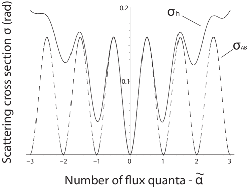
Figure 2: The scattering cross section $\sigma_{\textrm{h}}$ (solid line) in comparison with the Aharonov–Bohm scattering cross section ${\sigma}_{\textrm{AB}}$ (dashed line) as functions of the number of flux quanta $-\tilde{\alpha}$. For calculation we used $b/\omega\hbar=0.2$, $kh=100$ rad, $M=900$, $\chi=\piup/15$ rad.

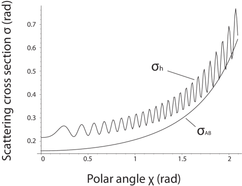
Figure 3: The angular dependence of the scattering cross section $\sigma_{\textrm{h}}(\chi)$; $\chi=0$ indicates the direction opposite to the incident beam. Smooth line is the Aharonov–Bohm scattering cross section, ${\sigma}_{\textrm{AB}}(\chi)$. For calculation we used $b/\omega\hbar=0.2$, $kh=100$ rad, $M=600$, $\tilde{\alpha}=3.5$.

The expression (3.8) is derived by using the asymptotics of the Bessel functions by type (3.5) that are valid only when the argument of the Bessel function is much larger than the index. For this reason, the expression (3.8) is not suitable for numerical calculations that use a finite sum instead of infinite. Hence, we construct a formula for calculations using the exact expressions for the wave functions, (3.2) and (3.6), and representation (3.1). Namely,

$$\mathcal{F}_{\textrm{h}}=\sqrt{kh}\exp(-\mathrm{i}kh)\left[\sum_{m=-M}^{M}(-\mathrm{i})^{\nu}J_{\nu}(kh)\exp(\mathrm{i}m\chi)-\exp(-\mathrm{i}kh\cos\chi-\mathrm{i}\tilde{\alpha}\chi)\right],$$ (4.1)

where $M$ is a maximum value of $m$ to which the numerical summation is performed. The scattering pattern on the screen is determined by the cross section $\sigma_{\textrm{h}}=\mathcal{F}_{\textrm{h}}\mathcal{F}_{\textrm{h}}^{*}$ which is the probability of a particle to be scattered through a given azimuthal angle $\chi$.

Numerical results for the scattering cross section $\sigma_{\textrm{h}}$ are given in figures 2 and 3 along with ${\sigma}_{\textrm{AB}}$ for comparison. As it is clearly seen from figure 2, the Aharonov–Bohm scattering cross section, ${\sigma}_{\textrm{AB}}$, vanishes for every integer $\tilde{\alpha}$ that corresponds to an integer number of flux quanta. By contrast, ${\sigma}_{\textrm{h}}$ is nonzero in the presence of any nonzero magnetic flux through the solenoid. In figure 3 there is shown the dependence of the scattering cross section on the azimuthal angle $\chi$. The Aharonov–Bohm scattering gives a smooth distribution of particles on the screen increasing from the center to the edges as ${\cos^{-2}(\chi/2)}$, see expression (3.10). The angular dependence of ${\sigma}_{\textrm{h}}$ is much more complicated and leads to the appearance of bands on the screen. The reason here is the different scattering of partial cylindrical waves with different values of the azimuthal number $m$.

In summary, the manifestations of the Aharonov–Bohm effect in systems described by the generalized Schrödinger equation loses its discreteness. The magnetic flux through the isolated region causes the scattering of particles for any nonzero value of the total flux. In real systems the effect can be attributed to the complex interaction with another particle system which leads to the emergence of new channels of scattering.

5 Conclusions

To conclude, let us make some remarks on possible applications of the model problem. Lagrangian density (2.1) appears in the study of quantum many-particle systems with nonconserved number of particles by reducing the problem to effective single-particle equations. First, it is important to notice that approximating Hamiltonian for a homogeneous electron gas in the Bardeen–Cooper–Schrieffer theory contains a $b$-proportional term (abnormal pairing potential) associated with the attraction between particles [19]. For this term to be non-zero, it is necessary that the electrons should be connected with the other particles, because the usual Coulomb interaction leads only to repulsion. In superconducting systems, the basic cause of the abnormal electron pairing is the electron-phonon interaction. However, relevant single-particle equations, known as the Bogolyubov equations, are not equivalent to the generalized Schrödinger equation (2.2). Therefore, the model problem considered in the article is not applicable to the fermion systems. More promising in this regard is the problem of the weakly nonideal Bose gas. Its condensate wave function satisfies the Gross–Pitaevskii equation. Linearized equations for small oscillations of the condensate wave function are of the form (2.4) where $a=b=\mu$ is the chemical potential [20]. The spectrum of the excitations coincides with the expression (2.10).

Another application area is the study of spin waves in the presence of topological solitons in the two-dimensional model of the Heisenberg ferromagnet. The Landau–Lifshitz equations describing the magnon dynamics on the soliton background can be presented in the form (2.2) with dimensionless potentials $a$ and $b$ tending to constant values at distances $r\gg l_{0}$, where $l_{0}$ is a characteristic length scale. Values of $a$ and $b$ are different for each specific system: in the case of a vortex in the easy-plane ferromagnet $a=b=1/2$, see [12]; in the easy-cone state of uniaxial magnets with comparable second-order and fourth-order anisotropy $a=b=\sin^{2}2\bar{\theta}/4$, where $\bar{\theta}$ is the opening angle of the cone, see [16]. The “mass” $m_{0}$ as well as the characteristic length $l_{0}$, which defines the limits of the validity of the theory, are expressed in terms of the exchange and anisotropy constants and the saturation magnetization. The role of the vector potential $\mathbf{A}$ is played by the vector $q\cos\theta_{0}/r\mathbf{e}_{\chi}$, where $q$ is the topological charge and $\theta_{0}$ is the polar angle of the soliton solution. This expression is convenient for either the vortex [12] or the Belavin–Polyakov soliton [22, 23], for the skyrmion vector potential additionally includes a term proportional to $\sin\theta_{0}$ and the Dzyaloshinskii–Moriya momentum [17]. For the most of the magnon modes, the wave function strongly decreases with the distance from the soliton core, i.e., magnons can be regarded as being apart from the core region. Thus, the continuous Aharonov–Bohm scattering takes place in the systems. In the finite geometry, it results in the splitting of magnon modes.

6 Acknowledgement

The author is deeply grateful to B.A. Ivanov for suggesting the problem and many helpful discussions.

Ukrainian 0

Íåïåðåðâíèé åôåêò Ààðîíîâà-Áîìà Â.Î. Óçóíîâà

             
Iíñòèòóò ôiçèêè ÍÀÍ Óêðà¿íè, ïðîñï. Íàóêè, 46, 03028 Êè¿â, Óêðà¿íà

References

- [1] Aharonov Y., Bohm D., Phys. Rev., 1959, 115, No. 3, 485–491, doi:10.1103/PhysRev.115.485.
- [2] Kretzschmar M., Z. Physik, 1965, 158, No. 1, 84–96, doi:10.1007/BF01381305.
- [3] Olariu S., Popescu I.I., Rev. Mod. Phys., 1985, 57, No. 2, 339–436, doi:10.1103/RevModPhys.57.339.
- [4] Brown R.A., J. Phys. A: Math. Gen., 1985, 18, No. 13, 2497–2508, doi:10.1088/0305-4470/18/13/025.
- [5] Brown R.A., J. Phys. A: Math. Gen., 1987, 20, No. 11, 3309–3326, doi:10.1088/0305-4470/20/11/034.
- [6] Kobe D.H., Liang J.Q., Phys. Rev. A, 1988, 37, No. 4, 1133–1140, doi:10.1103/PhysRevA.37.1133.
- [7] Sheka D.D., Mertens F.G., Phys. Rev. A, 2006, 74, 052703 (5 pages), doi:10.1103/PhysRevA.74.052703.
-
[8]
Rastelli G., Houzet M., Glazman L., Pistolesi F., C. R. Phys., 2012, 13, No. 5, 410–425,
doi:10.1016/j.crhy.2012.03.001. - [9] Skorobagatko G.A., Condens. Matter Phys., 2018, 21, No. 2, 23703 (8 pages), doi:10.5488/CMP.21.23703.
-
[10]
Shekhter R.I., Gorelik L.Y., Glazman L.I., Jonson M., Phys. Rev. Lett., 2006, 97, No. 15, 156801,
doi:10.1103/PhysRevLett.97.156801. -
[11]
Ivanov B.A., Schnitzer H.J., Mertens F.G., Wysin G.M., Phys. Rev. B, 1998, 58, No. 13,
8464–8474,
doi:10.1103/PhysRevB.58.8464. - [12] Sheka D.D., Yastremsky I.A., Ivanov B.A., Wysin G.M., Mertens F.G., Phys. Rev. B, 2004, 69, 054429 (13 pages), doi:10.1103/PhysRevB.69.054429.
-
[13]
Sheka D.D., Ivanov B.A., Mertens F.G., Phys. Rev. B, 2001, 64, 024432 (15 pages),
doi:10.1103/PhysRevB.64.024432. -
[14]
Iwasaki J., Beekman A.J., Nagaosa N., Phys. Rev. B, 2014, 89, 064412 (7 pages),
doi:10.1103/PhysRevB.89.064412. - [15] Ivanov B.A., Wysin G.M., Phys. Rev. B, 2002, 65, 134434 (17 pages), doi:10.1103/PhysRevB.65.134434.
- [16] Uzunova V.A., Ivanov B.A., Low Temp. Phys., 2019, 45, 92–97, doi:10.1063/1.5082327, [Fiz. Nizk. Temp., 2015, 45, No. 1, 104–110 (in Russian)].
- [17] Schütte C., Garst M., Phys. Rev. B, 2014, 90, 094423 (13 pages), doi:10.1103/PhysRevB.90.094423.
- [18] Schroeter S., Garst M., Low Temp. Phys., 2015, 41, 817 (10 pages), doi:10.1063/1.4932356, [Fiz. Nizk. Temp., 2015, 41, No. 10, 1043–1053].
-
[19]
De Gennes P.G., Superconductivity of Metals and Alloys, CRC Press, Boca Raton, 1999,
doi:10.1201/9780429497032, [Mir, Moscow, 1968 (in Russian)]. - [20] Lifshitz E.M., Pitaevskii L.P., Statistical Physics, Part 2: Theory of the Condensed State, Vol. 9, Oxford, 1980, [Nauka, Moscow, 1978 (in Russian)].
-
[21]
Bogolyubov N.N. (Jr.), A Method for Studying Model Hamiltonians, Pergamon Press, Oxford, New York, 1972,
doi:10.1016/C2013-0-02470-X, [Nauka, Moscow, 1974 (in Russian)]. - [22] Ivanov B.A., JETP Lett., 1995, 61, No. 11, 917–920, [Pis’ma Zh. Éksp. Teor. Fiz., 1995, 61, 898–902 (in Russian)].
- [23] Ivanov B.A., Sheka D.D., JETP Lett., 2005, 82, No. 7, 489–493, doi:10.1134/1.2142872, [Pis’ma Zh. Éksp. Teor. Fiz., 2005, 82, No. 7, 489–493 (in Russian)].
Ukrainian \adddialect\l@ukrainian0 \l@ukrainian