Abstract

I impose the Newtonian criteria of inertial frames on the c.o.m. trajectories of massive objects undergoing spontaneous collapse of their wave function. The corresponding modification of the so far used stochastic Schrödinger equation eliminates the Brownian motion of the c.o.m., restores the exact inertial motion for free masses. For the collapse of Schrödinger cat states the Born rule is satisfied invariably. The proposed machinery comes from the radical assumption that, in the vicinity of the spontaneously localized mass, the stochastic fluctuations of the c.o.m. —inevitable in the collapse process— would drag the physical inertial frame with themselves. The perspective of a general theory is presented where the spontaneous-collapse-caused breakdown of local energy-momentum conservation could be remedied by altering the metric, resulting in collapse-induced curvature of the space-time.

Spontaneous Wave Function Collapse with Frame Dragging and Induced Gravity Lajos Diósi Lajos Diósi Correspondence: diosi.lajos@wigner.mta.hu

1 Introduction

Spontaneous collapse (SC) theories, reviewed in BasGhi03 ; Basetal13 , propose that emergence of classical data in quantum systems is spontaneous and universal, does not require quantum measurements. Spontaneous wave function collapses happen everywhere time-continuously. They recover the results of standard collapse if typical measurement setups are considered. Models of SC fulfill two particular requirements: i) macroscopic degrees of freedom themselves should not develop superposition of macroscopically different states and ii) if such state, the so-called Schrödinger cat state

$$|\psi\rangle=\alpha|\psi_{1}\rangle+\beta|\psi_{2}\rangle$$ (1)

with macroscopically different $|\psi_{1}\rangle,|\psi_{2}\rangle$ were somehow prepared then it should quickly get collapsed through a random process either to $|\psi_{1}\rangle$ or to $|\psi_{2}\rangle$ with the probabilities $|\alpha|^{2}$, $|\beta|^{2}$ according to the Born-rule.

Available SC theories fulfill the above requirements at a cost of additional noise: the dynamics of $|\psi\rangle$ is charged by a diffusive motion in the Hilbert space which is mandatory consequence of the SC mechanisms. This means not only the non-conservation of momenta and energy but even an eternal increase of the latter.

Here I am going to outline a novel concept where SC is combined with the redefinition of the local inertial frame in such a way that the conservation of momentum in c.o.m. motion of massive objects is restored. Sec. 2 recapitulates the c.o.m. dynamics of quantized massive objects according to SC theories, Sec. 3 explains our motivations to include drag of the local inertial frame, Sec. 4 derives, Sec. 5 analyses the drag-related modifications of equations learned in Sec. 2. The principles of a general theory are outlined in Sec. 6, predicting a possible mechanism of induced gravity. Sec. VII contains discussion and summary.

2 Spontaneous Collapse

SC theories are microscopic theories, slightly modifying standard non-relativistic many-body Schrödinger equations in such a way that the modification remains ignorable at atomic scales and it gets amplified for massive degrees of freedom. For the c.o.m. wave function of a mass $M$, the Schrödinger equation acquires a small but significant nonlinearity and stochasticity (exactly as if the c.o.m. position $\hat{x}$ were under continuous position monitoring Dio88a , cf. Sec. 3, too). The corresponding stochastic Schrödinger equation (SSE) of the state $|\psi\rangle$ —in one spatial dimension for simplicity— reads:

$$d|\psi\rangle=-\frac{i}{\hbar}\hat{H}|\psi\rangle dt-\frac{D}{\hbar^{2}}\hat{x}_{c}^{2}|\psi\rangle dt+\frac{\sqrt{2D}}{\hbar}\hat{x}_{c}|\psi\rangle dW,$$ (2)

where $\hat{H}=\frac{1}{2}\hat{p}^{2}/M$ is the Hamiltonian and $\hat{x}_{c}=\hat{x}-\langle\hat{x}\rangle$ where the brackets $\langle.\rangle$ will denote the expectation values in state $|\psi\rangle$. The stochastic term is driven by the standard Wiener process $W_{t}$. The strength $D$ of the nonlinear stochastic modification depends on the parameters of the given microscopic model of SC, is growing with $M$ but remains extreme small even for macroscopic masses. (Ref. Heletal17 used the precise acceleration detection of the LISA pathfinder’s $M\sim 2kg$ free test mass to put an upper bound $\sim 10^{-22}cm^{2}/s^{3}$ on $D/M^{2}$.) If we consider the noise-averaged evolution, it turns out that the nonlinearities of the SSE cancel and we are left with the linear master equation for the density matrix ${\hat{\rho}}$:

$$\frac{d{\hat{\rho}}}{dt}=-\frac{i}{\hbar}[\hat{H},{\hat{\rho}}]-\frac{D}{\hbar^{2}}[\hat{x},[\hat{x},{\hat{\rho}}]].$$ (3)

An unavoidable feature of spontaneous collapse is the eternal increase of the average kinetic energy just like in classical diffusion with diffusion constant $D$:

$$\frac{d}{dt}\mbox{tr}(\hat{p}^{2}{\hat{\rho}})=-\frac{D}{\hbar^{2}}\langle[\hat{x},[\hat{x},\hat{p}^{2}]]\rangle=2D.$$ (4)

The diffusive motion itself is problematic conceptually because of momentum non-conservation. Solving the SSE (2), the picture gets even worse. There is diffusion in both momentum and position of the c.o.m. Dio88b :

$$d\langle\hat{x}\rangle = \frac{\langle\hat{p}\rangle}{M}dt+\frac{\sigma^{2}}{\hbar}\sqrt{8D}dW,$$ (5)

$$d\langle\hat{p}\rangle = R\sqrt{8D}dW,$$ (6)

where $\sigma^{2}=\langle\hat{x}_{c}^{2}\rangle$ and $R=\hbar^{-1}\mbox{Re}\langle\hat{x}_{c}\hat{p}_{c}\rangle$. While momentum diffusion (Brownian motion) is a common phenomenon classically as well, position diffusion is not, it corresponds to discontinuity of the spatial trajectory. But for sure, it is legitimate quantum mechanically, see our next Section.

3 The new idea: frame-drag

Since SC is utilizing its analogy with standard (and time-continuous) collapse (cf. Dio18 ), let us recollect what standard quantum theory teaches us about standard collapse. Consider a broad wave function and its standard collapse caused by a quantum measurement of position $\hat{x}$. The measurement localizes (collapses) the wave function at a random location, the localization width depends on the precision of the measurement device. The trajectory $\{\langle\hat{x}\rangle_{t},\langle\hat{p}\rangle_{t}\}$, let’s call it the classical trajectory, becomes discontinuous at the time of collapse and the kinetic energy $\frac{1}{2}\langle\hat{p}^{2}\rangle/M$ gets suddenly increased. These discontinuities and non-conservation of energy and momentum are all legitimate consequences of standard collapse in interaction with the measurement device. In standard theory of time-continuous measurement these features of one-shot collapse do survive. If the c.o.m. coordinate $\hat{x}$ is observed in a time-continuous way Dio88a —monitored, in other words— yielding the noisy signal

$$x_{t}=\langle\hat{x}\rangle_{t}+\frac{\hbar}{\sqrt{8D}}\frac{dW_{t}}{dt},$$ (7)

then the monitored state satisfies exactly the SSE (2) of SC where the parameter $D$ depends on the precision of the monitoring device. In this case diffusion of the classical trajectory $\{\langle\hat{x}\rangle_{t},\langle\hat{p}\rangle_{t}\}$ is a real effect . According to pilot arguments in Sec. 7, the well-known anomalies of nonlinear quantum theories this time are regularly suppressed just by the SC mechanism. If not in its SSE (2), why is SC different from collapse process under standard monitoring? SC is proposed to happen universally, everywhere and every time, and without the presence of monitoring devices. This makes violation of energy-momentum conservation universal, the diffusive classical trajectories and the constant gain of kinetic energy are also universal.

And this universality is exactly the point where I start from, toward a refined concept of SC and a modified SSE, to maintain continuity of spatial trajectory $\langle\hat{x}\rangle_{t}$ and conservation of momentum $\langle\hat{p}\rangle_{t}$ as well.

In Newtonian physics, an inertial frame is defined by the fact that in it free masses will move along straight lines at constant speeds. If they do not, then we are in the wrong frame and we have to redefine the coordinates $x,y,z$. Now, if we take quantization of the objects into the account, and we assume SC, then any free mass will slowly diffuse away from what we think in our frame to be inertial motion. Let us stick to the Newtonian definition and conclude that our frame is not the inertial one, our coordinates are not the Cartesian ones! Can we redefine our coordinate $x$ (and $y,z$ in the general case) in such a way that any free mass trajectory under SC move at constant speed (and along a straight line in full 3d)? In fact we can do so, provided the masses are far enough from each other. Then we redefine their local frames assuming that the diffusive (stochastic) part of the classical trajectory drags the local inertial frame, i.e., in a certain vicinity of the given mass we redefine the coordinates $x,y,z$ (cf. Fig. 1).

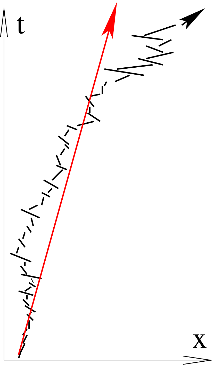
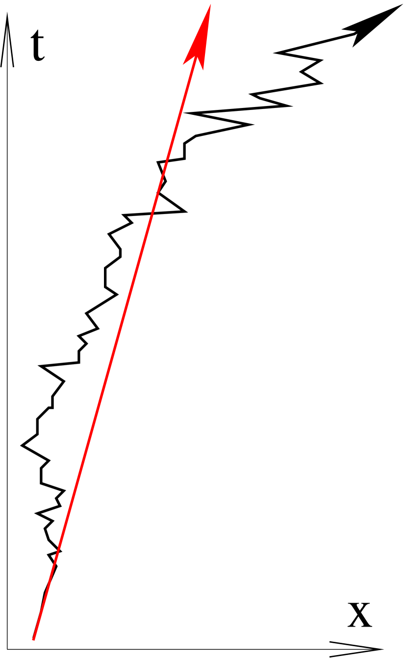
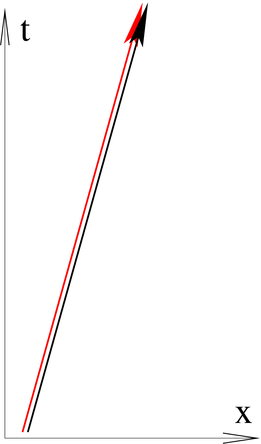
Figure 1: C.o.m. trajectory of classical inertial motion (red), c.o.m. trajectory $\langle\hat{x}\rangle_{t}$ of quantized motion under spontaneous collapse (black, L), after frame-shifts (black, M), and after frame-boosts (black, R).

4 Spontaneous collapse with frame-drag

We start from the SSE (2) and the diffusive trajectory equations (5,6). As said above, we assume that the mass drags the local frame with itself to the extent that in the new frame the diffusive part of the classical trajectory disappears. Namely, the frame will be shifted by the distance $du$ and boosted by the velocity $dv$, where

$$du = vdt+\frac{\sigma^{2}}{\hbar}\sqrt{8D}dW,$$ (8)

$$dv = \frac{1}{M}R\sqrt{8D}dW.$$ (9)

Then in the new frame the infinitesimal evolution of the state gets two factors:

$$|\psi\rangle+d|\psi\rangle = \exp\left\{-\frac{i}{\hbar}[R\hat{x}_{c}-\hbar^{-1}\sigma^{2}\hat{p}_{c}]\sqrt{8D}dW\right\}\times$$ (10)

$$\times \left\{1-\frac{i}{\hbar}\hat{H}dt-\frac{D}{\hbar^{2}}\hat{x}_{c}^{2}dt+\frac{\sqrt{2D}}{\hbar}\hat{x}_{c}dW\right\}|\psi\rangle.$$

The SSE (2) evolves the initial state $|\psi\rangle$ first, and the unitary factor of frame-drag (8,9) evolves it subsequently (see same calculation already in Ref. Dio88b ). The resulting SSE reads

$$d|\psi\rangle=-\frac{i}{\hbar}\hat{H}|\psi\rangle dt - \frac{D}{\hbar^{2}}\left(\hat{x}_{c}^{2}+4[R\hat{x}_{c}-\hbar^{-1}\sigma^{2}\hat{p}_{c}]^{2}+4i[R\hat{x}_{c}-\hbar^{-1}\sigma^{2}\hat{p}_{c}]\hat{x}_{c}\right)|\psi\rangle dt$$ (11)

$$+ \frac{\sqrt{2D}}{\hbar}(\hat{x}_{c}-2i[R\hat{x}_{c}-\hbar^{-1}\sigma^{2}\hat{p}_{c}])|\psi\rangle dW.$$

Comparing it with the old SSE (2), we recognize the new terms coming from the frame-drag. The equation can be rewritten into a compact form

$$d|\psi\rangle = -\frac{i}{\hbar}\left(\hat{H}+\hat{H}_{\psi}\right)|\psi\rangle dt-\frac{D}{\hbar^{2}}{\hat{A}}_{c}^{\dagger}{\hat{A}}_{c}|\psi\rangle dt+\frac{\sqrt{2D}}{\hbar}{\hat{A}}_{c}|\psi\rangle dW,$$ (12)

$$\hat{H}_{\psi} = \frac{4D}{\hbar}(R\hat{x}_{c}^{2}-\sigma^{2}{\hat{R}}),$$ (13)

$${\hat{A}}_{c} = \hat{x}_{c}-2i[R\hat{x}_{c}-\hbar^{-1}\sigma^{2}\hat{p}_{c}].$$ (14)

With notation $\hat{R}=\hbar^{-1}\mbox{Herm}\hat{x}_{c}\hat{p}_{c}$, we defined the nonlinear Hamiltonian $\hat{H}_{\psi}$ and introduced the “Lindbladian” ${\hat{A}}_{c}$. The frame-drag induced a new Hamiltonian (13) proportional to the small diffusion parameter $D$. When $R>0$ and $\sigma^{2}$ is not too large, the induced Hamiltonian $\hat{H}_{\psi}$ is gauge-equivalent with a self-attracting harmonic potential responsible for localization around $\langle\hat{x}\rangle$.

Whether a master equation, a modification of (3) exists or it does not? If the initial state is ${\hat{\rho}}=|\psi\rangle\langle\psi|$ then we have

$$\frac{d{\hat{\rho}}}{dt}=-\frac{i}{\hbar}[\hat{H}+\hat{H}_{\psi},{\hat{\rho}}]+\frac{2D}{\hbar^{2}}\left({\hat{A}}_{c}{\hat{\rho}}{\hat{A}}_{c}^{\dagger}-\mbox{Herm}{\hat{A}}_{c}^{\dagger}{\hat{A}}_{c}{\hat{\rho}}\right).$$ (15)

This looks like a dissipative Lindblad master equation. But, most importantly, this is only valid at the initial time when ${\hat{\rho}}$ is pure, because $\hat{H}_{\psi}$ and ${\hat{A}}_{c}$ depend on the pure state $|\psi\rangle$ and not on the average ${\hat{\rho}}$. The loss of the closed linear evolution of the density matrix is a warning that SC with frame-drag leads to an essentially nonlinear quantum theory, and this nonlinearity opens the door to major anomalies like non-physical action-at-a-distance Gis90 and the breakdown of the Born—von-Neumann statistical interpretation of $|\psi\rangle$, cf. Dio16 and references therein. We come back to this problem later in Sec. 7.

5 Dynamics in the dragged frames

To discuss the departure of the new SSE (12) from the old one (2) we follow two methods. First, we directly study the new one in Appendix A, to find that

$$\frac{d}{dt}\mbox{tr}(\hat{p}^{2}{\hat{\rho}}) = 2D(1-4R^{2}),$$ (16)

$$d\langle\hat{x}\rangle = \frac{\langle\hat{p}\rangle}{M}dt,$$ (17)

$$d\langle\hat{p}\rangle = 0.$$ (18)

The kinetic energy gain or loss in Eq. (16) depends on the position-momentum correlation $R$ which is zero for a real valued wave function when the rate of gain is $2D$ as in the SC without the drag, cf. Eq. (4). Below we see that $R$ tends asymptotically to $1/2$ and the kinetic energy will change no more. The Eqs. (17,18) are counterparts of Eqs. (5,6) — with no stochastic terms this time. It is straightforward to see that in the presence of a potential $V(\hat{x})$, our repeated derivation would modify Eq. (18) for $d\langle\hat{p}\rangle=-\langle V^{\prime}(\hat{x})\rangle$. This completes our statement: the classical trajectory $\{\langle\hat{x}\rangle_{t},\langle\hat{p}\rangle_{t}\}$ corresponds to classical motion (à la Ehrenfest).

Rather than to further discuss the SSE (12) itself, it is more convenient to consider the SSE (2) and invoke its known features that survive the drag invariably. According to (2), a broad initial wave packet starts to shrink immediately, shrinking has a random component. At the same time, the classical trajectory is charged by diffusive random fluctuations. Now, in the dragged frame, the process of shrinking of the wave packet remains the same, but the diffusive fluctuations of the trajectory go away, see Eqs. (17,18). It is known about the SSE (2) Dio88b that the solutions, after a transient period, converge asymptotically to the Gaussian soliton

$$\psi_{t}(x)=(2\pi\sigma_{\infty}^{2})^{-1/4}\exp\left(-(1-i)\frac{(x-\langle\hat{x}\rangle_{t})^{2}}{4\sigma_{\infty}^{2}}+\frac{i}{\hbar}\langle\hat{p}\rangle_{t}x\right)$$ (19)

at constant spread and correlation:

$$\sigma_{\infty}^{2}=\sqrt{\frac{\hbar^{3}}{8DM}},~{}~{}~{}~{}~{}~{}~{}~{}~{}R_{\infty}=1/2.$$ (20)

With the old SSE (2), the c.o.m. of the soliton remains subject of the phase-space diffusion (5,6):

$$d\langle\hat{x}\rangle = \frac{\langle\hat{p}\rangle}{M}dt+\sqrt{\frac{\hbar}{m}}dW,$$ (21)

$$d\langle\hat{p}\rangle = \sqrt{2D}dW,$$ (22)

but this time the coefficients are constants. In the dragged frames, i.e. with SSE (12), this diffusion disappears. After a transient period, the free mass wave packet becomes a soliton (cf. also Appendix A) and will move classically, like traveling free solitons used to.

If the initial state were a Schrödinger cat (1), where $|\psi\rangle_{1}$ and $|\psi\rangle_{2}$ are distant (suppose standing) wave packets then the SSE (2) predicts a quick collapse of the cat into one of the components, randomly and with the Born probabilities, respectively. Obviously the collapse itself happens the same way in the dragged frames as well. The only difference is that the c.o.m. will be preserved. E.g., if $x_{1}=\langle\hat{x}\rangle_{1}$ and $x_{2}=\langle\hat{x}\rangle_{1}$ stand for the respective quantum expectation values of $\hat{x}$ in the two distant wave packets in question, then $\langle\hat{x}\rangle=|\alpha|^{2}x_{1}+|\beta|^{2}x_{2}$ is the c.o.m. of the Schrödinger  cat and if the quick collapse happens, say, to $|\psi\rangle_{1}$ then it gets shifted from $x_{1}$ to the middle, i.e. to $\langle\hat{x}\rangle$. (Same happens with traveling wave packets $|\psi\rangle_{1},|\psi\rangle_{2}$, in the velocity space.)

We conclude that the particular requirements i)-ii) for SC, mentioned in Sec. 2, that are fulfilled by the available theories, will remain satisfied by the new SC model with frame-drag, with the bonus that, unlike in the old SC models, the classical trajectory $\{\langle\hat{x}\rangle_{t},\langle\hat{p}\rangle_{t}\}$ follows the classical equations of motion, also conservation of momentum $\langle\hat{p}\rangle_{t}$ and the continuity of the path $\langle\hat{x}\rangle_{t}$ become restored. Let us remark that we would try dragging the local clock-time too, with a desire if the mean kinetic energy would be conserved even in the transient period. Next Section outlines the principles of local energy-momentum conservation by local dragging $x,y,z,t$ and with possible “dragging” the local metric, too.

6 Principles of a general theory: induced gravity

As I said in Sec. 2, available SC models are microscopic and in terms of fields. Local frame-drags anticipate the necessity to use curvilinear coordinates. Dynamics in curvilinear coordinates are, for historic reasons, less common non-relativistically than relativistically. Hence I found it more convenient to consider a possible relativistic formalism of frame-drags first. Harnessed with the standard theory of metric in general coordinates, the notion of local inertial frames in the vicinity of distant masses, used in Secs. 3-4, becomes trivial. Also tailoring of distant local inertial frames is straightforward mathematically. Standard collapses are not invariant relativistically, thus a relativistic concept of SC is far from being established. Nonetheless, here I assume that there can be a related theory just for the sake of using the relativistic formalism of space-time structure.

Consider a flat space-time with Minkowski coordinates $\mathrm{x}^{a}$ and metric $\eta_{ab}$, which is the background for quantized relativistic fields of matter. The definition of a Minkowski inertial frame, whose non-relativistic limit is Newton’s definition in Sec. 3, can be formulated in terms of the energy-momentum tensor $T_{ab}$, by requiring that its divergence vanish:

$$\nabla_{b}T_{a}^{b}=0.$$ (23)

This is to be satisfied by $\hat{T}_{ab}$ after quantization of the relativistic fields. To think about relativistic SC theories, according to concepts in TilDio16 and earlier references therein, now we suppose the presence of a certain universal and spontaneous monitoring of the energy-momentum tensor $\hat{T}_{ab}(\mathrm{x})$ yielding the signal

$$T_{ab}(\mathrm{x})=\langle\hat{T}_{ab}(\mathrm{x})\rangle+\delta T_{ab}(\mathrm{x}),$$ (24)

where $\langle.\rangle$ stands for expectation value in the Heisenberg picture and $\delta T_{ab}(\mathrm{x})$ is a classical (colored) noise. Monitoring modifies the standard unitary evolution of the fields, the expectation values $\langle T_{ab}(\mathrm{x})\rangle$ themselves have stochastic components. The divergence $\nabla_{b}\hat{T}_{a}^{b}$ does no more vanish, neither does it so in mean:

$$\nabla_{b}\langle\hat{T}_{a}^{b}\rangle\neq 0.$$ (25)

We proceed in the spirit of Sec. 3 and decide that $\mathrm{x}^{a}$ are not the correct Minkowski coordinates. Similarly to what we did in Sec. 4, we could try frame-drag locally this time:

$$\mathrm{x}^{a}\rightarrow\mathrm{x}^{a}+\xi^{a}(\mathrm{x}),$$ (26)

to ensure $\nabla_{b}\langle\hat{T}_{a}^{b}(\mathrm{x})\rangle=0$ in the dragged coordinates. (In parenthesis, we mention an alternative: we could try to construct frame drag to ensure that the signal (24) satisfy $\nabla_{b}T_{a}^{b}=0$.) There is no guarantee that frame-drag gives us sufficient freedom to get rid of the divergence of $\langle\hat{T}_{ab}\rangle$. Fortunately, we can replace frame-drag by something more general, more plausible, and more convenient.

The concept in Sec. 3 says that the original Cartesian flat (here Minkowski) background metric is valid in the dragged coordinates. But we know that change of coordinates (26) at retaining the metric $\eta_{ab}$ is equivalent to retaining the coordinates and changing the metric :

$$\eta_{ab}\rightarrow\eta_{ab}-\nabla_{b}\xi_{a}-\nabla_{a}\xi_{b}+\mbox{higher order terms in }\xi.$$ (27)

And here we come to a turning point. We forget frame-drag (27) and allow for a general change of the metric:

$$\eta_{ab}\rightarrow\eta_{ab}+\delta g_{ab},$$ (28)

to ensure

$$\nabla_{b}^{covariant}\langle\hat{T}_{a}^{b}(\mathrm{x})\rangle=0$$ (29)

in the original coordinates. This gives us a much wider freedom, compared to frame-drag, to solve the task. We can change the space-time’s physical structure that frame-drags leave unchanged. If violation of energy-momentum conservation by SC goes away in a modified space-time structure then I talk about gravity induced by collapses.

There is no apriori guarantee that change of the metric can restore energy-momentum conservation (29) lost by SC. Even if this were the case, the induced space-time curvature may be different from Einstein’s that is sourced by masses, not by wave function collapses. The concept points anyway towards a new coupling between quantized matter and classical space-time — different from all previous high level proposals like the semiclassical Mol62 ; Ros63 , the Bohmian Str15 ; Lal19 , or the stochastic semiclassical TilDio16 ; TilDio17 couplings.

7 Difficulties, perspectives, summary

The essential nonlinearity, like that of our new SC proposal (cf. Sec. 3), is well-feared because of major anomalies it induces. These anomalies, on the other hand, require particular entangled states between distant systems. In our case, entanglement of the c.o.m. degrees of freedom of distant massive objects is required, otherwise the anomalies do not surface. This offers a loophole, specific to SC theory: such states are heavily suppressed by the very mechanism of SC.

Leading SC models are microscopic, like the DP model Dio89 ; Pen96 is (though cautious Roger Penrose advocates his “minimalist approach” without constructing detailed dynamics) and like the CSL model GhiPeaRim90 is. In the present proposal we discussed and modified the effective SC of the simplest massive macroscopic d.o.f. which are the c.o.m. of massive objects. It is not trivial how we can implement the concept of frame-drag and induced gravity at the microscopic scales. A creative approach can start from the elementary mechanism shown in Secs. 3-4. Alternative starting point can be the Newtonian limit of the general theory drafted in Sec. 6. A systematic test of both frame-drag and induced gravity on DP model inprep would enlighten whether the new concept is new physics or a deadlock.

The intrinsic —non-dynamical— combination between SC and gravity has been basic for the DP-model from its conception Dio89 ; Pen96 . Much later, this has been shown to be the unique combination of SC and semiclassical gravity that eliminates the essential nonlinearity of semiclassical gravity TilDio16 ; TilDio17 . But the derivation of an emergent Newtonian gravity from SC lacked the sufficient inspiration. The precursor of the present idea of restoring momentum-conservation and geodetic (inertial) motion of free masses under SC occurred ten years ago, led me to a sophisticated argument —with a bit of wishful thinking— for induced Newtonian gravity Dio09 . The present proposal of frame-drag, visioned from the Newtonian definition of inertial frames, points towards a new relationship between SC and gravity. While SC had been conceived as a model of emergence of classicality in a quantized Universe, it may be responsible for the emergence of gravity as well, as the title of Ref. Dio09 proposed literally.

In this work, we eliminate the well-known violation of classical equations of motion in the c.o.m. dynamics of masses under spontaneous wave funtion collapse, imposing suitable transformation of the reference frame coordinates, called frame-drag. We also outlined a general theory where the violation of the local energy-momentum conservation by spontaneous collapses can be removed by the suitable change of the space-time metric structure, contributing to a new concept of inducing gravity by collapses instead of sourcing it by masses. Relevance of this latter perspective has still to be confirmed or rejected by testing it on currently known spontaneous collapse models.

This research was funded by the National Research Development and Innovation Office of Hungary Projects Nos. 2017-1.2.1-NKP-2017-00001 and K12435, by EU COST Action CA15220, by the Foundational Questions Institute mini-grant.

Appendix A

Selected features of the SSE (12) —with definitions (13,14), and $\hat{H}=\frac{1}{2}\hat{p}^{2}/M)$— are derived below.

Proof of Eq. (16). The SSE (12) or, equivalently, the master equation (15) yields the following equation for the increment of $\mbox{tr}(\hat{p}^{2}{\hat{\rho}})$:

$$d\mbox{tr}(\hat{p}^{2}{\hat{\rho}})=\left\langle\frac{i}{\hbar}[\hat{H}_{\psi},\hat{p}^{2}]dt+\frac{D}{\hbar^{2}}(2{\hat{A}}_{c}^{\dagger}\hat{p}^{2}{\hat{A}}_{c}-\{{\hat{A}}_{c}^{\dagger}{\hat{A}}_{c},\hat{p}^{2}\})dt\right\rangle.$$ (30)

Work out the relationships:

$${[\hat{H}_{\psi},\hat{p}^{2}]} = 8iD(R\{\hat{x}_{c},\hat{p}\}-\hbar^{-1}\sigma^{2}\hat{p}_{c}\hat{p}),$$ (31)

$$2{\hat{A}}_{c}^{\dagger}\hat{p}^{2}{\hat{A}}_{c}-\{{\hat{A}}_{c}^{\dagger}{\hat{A}}_{c},\hat{p}^{2}\} = 2\hbar^{2}(1+4R^{2})-8\sigma^{2}\hat{p}_{c}\hat{p},$$ (32)

and insert them:

$$d\mbox{tr}(\hat{p}^{2}{\hat{\rho}})=\left\langle\frac{i}{\hbar}8iD(R\{\hat{x}_{c},\hat{p}\}-\hbar^{-1}\sigma^{2}\hat{p}_{c}\hat{p})+\frac{D}{\hbar^{2}}2\hbar^{2}(1+4R^{2})-8\sigma^{2}\hat{p}_{c}\hat{p}\right\rangle=2D(1-4R^{2}),$$ (33)

where we used the identity $\langle\{\hat{x}_{c},\hat{p}\}\rangle=2\hbar R$.

Proof of Eq. (17). The SSE (12) yields the following equation for the spatial trajectory:

$$d\langle\hat{x}\rangle=\left\langle\frac{i}{\hbar}[\hat{H}+\hat{H}_{\psi},\hat{x}]dt+\frac{D}{\hbar^{2}}(2{\hat{A}}_{c}^{\dagger}\hat{x}{\hat{A}}_{c}-\{{\hat{A}}_{c}^{\dagger}{\hat{A}}_{c},\hat{x}\})dt+\frac{\sqrt{2D}}{\hbar}(\hat{x}{\hat{A}}_{c}+{\hat{A}}_{c}^{\dagger}\hat{x})dW\right\rangle.$$ (34)

The free Hamiltonian $\hat{H}$ yields $(\langle\hat{p}\rangle/M)dt$, the other terms yield zero, since

$$\langle[\hat{H}_{\psi},\hat{x}]\rangle = 8iD\langle\sigma^{2}\hat{p}_{c}\rangle=0,$$ (35)

$$\langle 2{\hat{A}}_{c}^{\dagger}\hat{x}{\hat{A}}_{c}+\{{\hat{A}}_{c}^{\dagger}{\hat{A}}_{c},\hat{x}\}\rangle = \langle{\hat{A}}_{c}^{\dagger}[\hat{x},{\hat{A}}_{c}]+H.C.\rangle=-2\sigma^{2}\langle{\hat{A}}_{c}^{\dagger}\rangle+C.C.=0,$$ (36)

$$\langle\hat{x}{\hat{A}}_{c}+{\hat{A}}_{c}^{\dagger}\hat{x}\rangle = 2\langle\hat{x}\hat{x}_{c}\rangle-2\sigma^{2}=0.$$ (37)

Proof of Eq. (18). The SSE (12) yields the following equation for the momentum:

$$d\langle\hat{p}\rangle=\left\langle\frac{i}{\hbar}[\hat{H}_{\psi},\hat{p}]dt+\frac{D}{\hbar^{2}}(2{\hat{A}}_{c}^{\dagger}\hat{p}{\hat{A}}_{c}-\{{\hat{A}}_{c}^{\dagger}{\hat{A}}_{c},\hat{p}\})dt+\frac{\sqrt{2D}}{\hbar}(\hat{p}{\hat{A}}_{c}+{\hat{A}}_{c}^{\dagger}\hat{p})dW\right\rangle.$$ (38)

The r.h.s. vanishes since

$$\langle[\hat{H}_{\psi},\hat{p}]\rangle = 8iD\langle R\hat{p}_{c}-\sigma^{2}\hat{x}_{c}\rangle=0,$$ (39)

$$\langle 2{\hat{A}}_{c}^{\dagger}\hat{p}{\hat{A}}_{c}+\{{\hat{A}}_{c}^{\dagger}{\hat{A}}_{c},\hat{p}\}\rangle = \langle{\hat{A}}_{c}^{\dagger}[\hat{p},{\hat{A}}_{c}]+H.C.\rangle=-i\hbar(1-2iR)\langle{\hat{A}}_{c}^{\dagger}\rangle+C.C.=0,$$ (40)

$$\langle\hat{p}{\hat{A}}_{c}+{\hat{A}}_{c}^{\dagger}\hat{p}\rangle = \langle\{\hat{p},\hat{x}_{c}\}\rangle-2\hbar R=0.$$ (41)

Proof of static soliton solution:

$$\langle x|\psi\rangle=(2\pi\sigma_{\infty}^{2})^{-1/4}\exp\left(-(1-i)\frac{x^{2}}{4\sigma_{\infty}^{2}}\right).$$ (42)

Applying the SSE (12) to it, the stochastic term vanishes since

$${\hat{A}}_{c}|\psi\rangle=i(1-2R_{\infty})|\psi\rangle=0.$$ (43)

The yield of the deterministic terms reads:

$$(\hat{H}+\hat{H}_{\psi})|\psi\rangle = \left\{\frac{\hbar^{2}}{2M\sigma_{\infty}^{2}}-i\left(\frac{\hbar^{2}}{4M\sigma_{\infty}^{2}}-\frac{2D\sigma_{\infty}^{2}}{\hbar}\right)+\frac{2D}{\hbar}(2R_{\infty}-1)\hat{x}^{2}+i\left(\frac{\hbar^{2}}{4M\sigma_{\infty}^{4}}-\frac{4D}{2\hbar}\right)\hat{x}^{2}\right\}|\psi\rangle$$ (44)

$$= \frac{\hbar^{2}}{2M\sigma_{\infty}^{2}}|\psi\rangle.$$

References

References

- (1) Bassi, A.; Ghirardi, G.C. Dynamical reduction models. Phys. Rep. 2003, 379, 257–426.
- (2) Bassi, A.; Lochan, K.; Satin, S.; Singh, T.P.; Ulbricht, H. Models of wave-function collapse, underlying theories, and experimental tests. Rev. Mod. Phys. 2013, 85, 471–527.
- (3) Diósi, L. How to teach and think about spontaneous wave function collapse theories: not like before. In Collapse of the Wave Function; Gao, S., Ed.; Cambridge University Press, Cambridge, UK, 2018) pp. 3–11. arXiv:1710.02814
- (4) Diósi, L. Continuous quantum measurement and Ito-formalism. Phys. Lett. A 1988, 129, 419–423.
- (5) Diósi L. Classical-quantum coexistence: a ‘free will’ test. J. Phys. Conf. Ser. 2012, 361, 012028-(7).
- (6) Helou B.; Slagmolen, B.J.J.; McClelland, D.E.; Chen, Y. LISA pathfinder appreciably constrains collapse models. Phys. Rev. D 2017, 95, 084054.
- (7) Diósi, L. Localized solution of simple nonlinear quantum Langevin-equation. Phys. Lett. A 1988, 132, 233–236.
- (8) Gisin, N. Weinberg non-linear quantum-mechanics and supraluminal communications. Phys. Lett. A 1990, 143, 1–2.
- (9) Diósi, L. Nonlinear Schrödinger equation in foundations: summary of 4 catches. J. Phys. Conf. Ser. 2016 701, 012019-(5). arXiv:1602.03772 (erratum)
- (10) Diósi, L. Models for universal reduction of macroscopic quantum fluctuations. Phys. Rev. A 1989, 40, 1165–1174.
- (11) Penrose, R. On gravity’s role in quantum state reduction. Gen. Rel. Grav. 1996, 28, 581–600.
- (12) Ghirardi, G.C.; Pearle, P.; Rimini, A. Markov processes in Hilbert space and continuous spontaneous localization of systems of identical particles. Phys. Rev. A 1990, 42, 78–89.
- (13) Tilloy, A.; Diósi, L. Sourcing semiclassical gravity from spontaneously localized quantum matter. Phys. Rev. D 2016, 93, 024026-(12).
- (14) Tilloy, A.; Diósi, L. Principle of least decoherence for Newtonian semiclassical gravity. Phys. Rev. D 2017, 96, 104045-(6).
- (15) Møller, C. Les theories relativistes de la gravitation. CNRS, Paris, 1962.
- (16) Rosenfeld, L. On quantization of fields. Nucl. Phys., 1963, 40, 353.
- (17) Struyve, W. Semi-classical approximations based on Bohmian mechanics. arXiv:1507.04771 (2015).
- (18) Laloe, F. A model of quantum collapse induced by gravity. arXiv:1905.12047 (2019).
- (19) In preparation.
- (20) Diósi, L. Does wave function collapse cause gravity? J. Phys. Conf. Ser. 2009, 174, 012002-(6).