Astronomy Letters, 2019, Vol. 45, No 9, pp. 580–592.
Kinematics of Hot Subdwarfs from the Gaia DR2 Catalogue
V.V. Bobylev111e-mail: vbobylev@gaoran.ru and A.T. Bajkova
Pulkovo Astronomical Observatory, Russian Academy of Sciences,
Pulkovskoe sh. 65, St. Petersburg, 196140 Russia
Abstract—We have studied the kinematic properties of the candidates for hot subdwarfs (HSDs) selected by Geier et al. from the Gaia DR2 catalogue. We have used a total of 12 515 stars with relative trigonometric parallax errors less than 30%. The HSDs are shown to have different kinematics, depending on their positions on the celestial sphere. For example, the sample of low-latitude HSDs rotates around the Galactic center with a linear velocity km s-1. This suggests that they belong to the Galactic thin disk. At the same time, they lag behind the local standard of rest by km s-1 due to the asymmetric drift. The high-latitude () HSDs rotate with a considerably lower velocity, km s-1. Their lagging behind the local standard of rest is already km s-1. Based on the entire sample of 12 515 HSDs, we have found a positive rotation around the axis significantly differing from zero with an angular velocity km s-1 kpc-1. We have studied the samples of HSDs that are complete within kpc. Based on them, we have traced the evolution of the parameters of the residual velocity ellipsoid as a function of both latitude and coordinate The following vertical disk scale heights have been found: and pc from the low- and high-latitude HSDs, respectively. A new estimate of the local stellar density /kpc2 kpc-2 has been obtained for kpc from the high-latitude HSDs.
DOI: 10.1134/S1063773719080012
INTRODUCTION
The hot subdwarfs (sdO, sdB, sdOB) are located between the main sequence and the white dwarf sequence on the Hertzsprung–Russell diagram. Their peculiarity is core helium burning. Such stars were first detected by Humason and Zwicky (1947) while studying super-bright blue stars near the North Galactic Pole. Further spectroscopic studies revealed a hydrogen underabundance in many hot subdwarfs. Their temperature and surface gravity measurements (Greenstein and Sargent 1974) allowed the proper positions of such stars on the Hertzsprung–Russell diagram to be determined. More specifically, they occupy a compact region at the blue end of the horizontal branch, thereby being a late evolutionary stage of massive stars.
The formation of hot subdwarfs (HSDs) is explained, for example, by the loss of hydrogen by a red giant from its outer layers before the reactions involving helium begin in the core. The cause of this loss is not completely clear, but it is hypothesized that this is the result of interaction between the stars in a binary system. It is assumed that single HSDs can result from a merger of two white dwarfs.
At present, there is extensive literature on the investigation of single HSDs (Randall et al. 2016; Latour et al. 2018) and binary systems with HSDs (Kupfer et al. 2015; Vos et al. 2018). Their study can help in understanding the evolutionary peculiarities of other galaxies, the presence of an ultraviolet excess, in particular (Han et al. 2007), galactic globular clusters (Lei et al. 2016), the stellar evolution (Fontaine et al. 2012), and can help in searching for the progenitors of type Ia supernovae (Geier et al. 2007).
Only with the appearance of highly accurate astrometric data from the Gaia space experiment (Brown et al. 2016, 2018; Lindegren et al. 2018) has a largescale statistical analysis of various Galactic subsystems, in particular, a statistical and kinematic analysis of HSDs, become possible. The methods of searching for and identifying of such stars in largescale surveys are being developed (Bu et al. 2017); the first big catalogues of HSDs containing the necessary data on tens of thousands of stars have appeared (Geier et al. 2019).
Samples of protoplanetary nebulae (PPNe) and planetary nebulae (PNe) were studied in Bobylev and Bajkova (2017a) and Bobylev and Bajkova (2017b), respectively. Based on three laws of the density distribution, we determined the vertical disk scale height and estimated the Galactic rotation parameters. Many HSDs are at a more advanced evolutionary stage compared to PPNe and PNe, which is important for studying the various stages of stellar evolution.
The goal of this paper is to analyze the kinematics and spatial distribution of a large sample of HSD candidates. Such a sample of 39 800 stars has recently been produced by Geier et al. (2019) using data from the Gaia DR2 catalogue (Brown et al. 2018; Lindegren et al. 2018) and a number of photometric sky surveys.
DATA
In this paper we use the catalogue by Geier et al. (2019). It contains 39 800 HSD candidates selected from the Gaia DR2 catalogue in combination with several ground-based multiband photometric sky surveys. HSDs of spectral types O and B, late- B stars in the blue part of the horizontal branch, hot post-AGB stars, and PN central stars are expected to constitute the majority of candidates. The authors of the catalogue believe that the contamination by cooler stars is about 10%. The selected HSDs are distributed over the entire celestial sphere. According to the estimates by Geier et al. (2019), the catalogue is complete to a distance of 1.5 kpc, except for the narrow region near the Galactic plane and the zones with the Magellanic Clouds.
For each star this catalogue gives the trigonometric parallax and two proper motion components, and . There are no radial velocities. Extensive photometric information is also available.
Of course, the radial velocities have been measured for several hundred HSDs. Note, for example, the catalogue of radial velocities for such stars in close binary systems by Geier et al. (2015) or Kupfer et al. (2015). In those cases where it is possible to construct the orbit of a binary or multiple system, the systemic velocity is usually determined with an error of 1–5 km s-1. However, for such a large number as 39 800 HSDs no highly accurate radial velocities have been measured so far.
In this paper, to determine the kinematic parameters, we took stars with relative trigonometric parallax errors less than 30%. In addition, the zero-point correction was added to the Gaia DR2 parallaxes; thus, the new stellar parallax is mas. The necessity of applying this systematic correction mas (here the minus means that the correction should be added to the Gaia DR2 stellar parallaxes to reduce them to the standard) was first pointed out by Lindegren et al. (2018) and confirmed by Arenou et al. (2018). Slightly later, having analyzed various highly accurate sources of distance scales, Stassun and Torres (2018), Riess et al. (2018), Zinn et al. (2018), and Yalyalieva et al. (2018) showed the correction to be mas with an error of several units of the last decimal digit.
METHODS
In this paper we consider stars only with the proper motions, because there is no information about the radial velocities in the catalogue by Geier et al. (2019). Thus, two tangential velocity components are known from observations, and along the Galactic longitude and latitude respectively, expressed in km s-1. Here, the coefficient 4.74 is the ratio of the number of kilometers in an astronomical unit to the number of seconds in a tropical year, and is the stellar heliocentric distance in kpc that we calculate via the stellar parallax The proper motion components and are expressed in mas yr-1.
To determine the parameters of the Galactic rotation curve, we use the equations derived from Bottlinger’s formulas in which the angular velocity is expanded into a series to terms of the second order of smallness in
| (1) |
| (2) |
where is the distance from the star to the Galactic rotation axis (cylindrical radius vector):
| (3) |
is the angular velocity of Galactic rotation at the solar distance the parameters and are the corresponding derivatives of the angular velocity, and . Apart from the rotation around the Galactic axis (described by the parameter ), in this paper we also consider the angular velocities of rotation around the and axes described by the parameters and , respectively.
Note that in this paper the signs of the unknowns are taken in such a way that the positive rotations occur from the axis to from to and from to Thus, the angular velocity of Galactic rotation will be negative, in contrast to many other papers (Rastorguev et al. 2017; Vityazev et al. 2017; Bobylev and Bajkova 2017a), where, for convenience, it is deemed positive.
The interest in and stems from the following factors. First, this can be a slight residual rotation of the Gaia DR2 reference frame relative to the inertial reference frame. Second, this can be a reflection of the Galactic warp or other processes causing the vertical oscillations of stars in the Galaxy. A uniform distribution of the stars being analyzed over the celestial sphere is required for a reliable determination of the parameters and . Dwarfs and subdwarfs are well suited for solving this problem.
In the system of conditional equations (1)–(2) eight unknowns are to be determined: and . We find their values by solving the conditional equations by the least-squares method (LSM). Weights of the form and are used, where is the “cosmic” dispersion (for each sample we find its value in advance to be close to the error per unit weight obtained by presolving the equations), and are the errors in the corresponding observed velocities. is comparable to the root-mean-square residual (the error per unit weight) calculated by solving the conditions equations (1)–(2). The solution is sought in several iterations by applying the criterion to exclude the stars with large residuals.
Note several papers devoted to determining the mean Galactocentric distance of the Sun using its individual determinations made in the last decade by independent methods. For example, kpc (Valleé 2017), kpc (de Grijs and Bono 2017) or kpc (Camarillo et al. 2018). Based on these reviews, in this paper we adopt kpc.
Residual Velocity Ellipsoid
We estimated the dispersion of the stellar residual velocities using the following well-known method (Ogorodnikov 1965). Let be the velocities along the coordinate axes and Let us consider the six second-order moments
| (4) |
which are the coefficients of the equation for the surface
| (5) |
and also the components of the symmetric tensor of moments of the residual velocities:
| (6) |
To determine the values in this tensor in the absence of radial-velocity data, the following three equations are used:
| (7) |
| (8) |
| (9) |
which are solved by the least-squares method for the six unknowns and . The eigenvalues of the tensor (6) are then found from the solution of the secular equation
| (10) |
The eigenvalues of this equation are equal to the reciprocals of the squares of the semiaxes of the velocity moment ellipsoid and, at the same time, the squares of the semiaxes of the residual velocity ellipsoid:
| (11) |
We found the directions of the main axes of the tensor (10), and from the relations:
| (12) |
| (13) |
Exponential Density Distribution
In the case of an exponential distribution of the density along the coordinate axis, we have
| (14) |
where is the normalization constant; is the mean value calculated from the coordinates of the sample stars, which reflects the well-known fact of the Sun’s elevation above the Galactic plane; and is the vertical scale height. The observed histogram of the distribution of stars along the axis is described by an analogous expression:
| (15) |
where is the normalization coefficient.
The surface density of gravitating matter within a distance from the Galactic plane can be found from the following relation:
| (16) |
where the gravitational constant is taken to be equal to one. Following the approach by Korchagin et al. (2003) based on the solution by Spitzer (1942) for a self-gravitating disk, we have
Given , the mean vertical velocity the scale height and the Oort constants and we can estimate the surface density from the relation
| (17) |
| Parameters | All stars | ||
|---|---|---|---|
| km s-1 | |||
| km s-1 | |||
| km s-1 | |||
| km s-1 kpc-1 | |||
| km s-1 kpc-2 | |||
| km s-1 kpc-3 | |||
| km s-1 kpc-1 | |||
| km s-1 kpc-1 | |||
| km s-1 | 39.6 | 30.5 | 50.2 |
| 7128 | 3767 | 3361 | |
| kpc | 1.41 | 1.35 | 1.48 |
| km s-1 kpc-1 | |||
| km s-1 kpc-1 | |||
| km s-1 | |||
| km s-1 | |||
| km s-1 | |||
| km s-1 | |||
| km s-1 kpc-1 | |||
| km s-1 kpc-2 | |||
| km s-1 kpc-3 | |||
| km s-1 kpc-1 | |||
| km s-1 kpc-1 | |||
| km s-1 | 44.1 | 33.1 | 55.9 |
| 12515 | 6690 | 5825 | |
| kpc | 1.90 | 1.83 | 1.97 |
| km s-1 kpc-1 | |||
| km s-1 kpc-1 | |||
| km s-1 |
is the number of stars used, is the mean distance of the sample of stars, and is the error per unit weight.
RESULTS AND DISCUSSION
Galactic Rotation Parameters
We have run into the fact that the HSDs under consideration have different kinematic properties, depending on their positions in the Galaxy. Therefore, the entire sample was divided into two groups, depending on the absolute value of the Galactic latitude: low-latitude and high-latitude stars.
The kinematic parameters found for these stars are given in Table 1. Apart from the eight sought for kinematic parameters, it gives the following: the mean distance of the sample of stars , the error per unit weight that we estimate when seeking the LSM solution of the system of conditional equations (1)–(2), the Oort constants and that we calculate based on the following relations:
| (18) |
and the linear rotation velocity of the Galaxy at the solar distance . When calculating the kinematic parameters presented in Table 1, we took the stars from the interval 0.5–6 kpc and rejected the stars with large (more than 60 km s-1) random measurement errors of their proper motions.
The separation in relative parallax error was made for the following reasons. On the one hand, using the stars with relative trigonometric parallax errors less than 30% allows us to use a large number of objects and to estimate the sought-for parameters with smaller errors. On the other hand, the sample of stars with parallax errors less than 15% allows more local parameters, in particular, more reliable estimates of the velocities and to be obtained.
First note the parameters that describe the kinematics of the most rapidly rotating Galactic subsystems. For example, based on 130 masers with measured VLBI trigonometric parallaxes, Rastorguev et al. (2017) found the following quantities: km s-1, km s-1 kpc-1, km s-1 kpc-2, km s-1 kpc-3, and km s-1 (for the derived kpc). Based on a sample of young open star clusters with the proper motions and distances from the Gaia DR2 catalogue, Bobylev and Bajkova (2019) obtained the following estimates: km s-1, km s-1 kpc-1, km s-1 kpc-2, and km s-1 kpc-3, where km s-1 (for the adopted kpc).
The linear velocity km s-1 inferred from the low-latitude HSDs (the upper part of Table 1) suggests that this population of stars belongs to the thin disk. At the same time, the velocity km s-1 derived from them shows that they lag behind the local standard of rest by km s-1 due to the so-called asymmetric drift. One of the reliable present-day determinations of the parameters of the peculiar solar motion relative to the local standard of rest was made by Schönrich et al. (2010), km s-1. For all of the older Galactic objects their lagging behind the local standard of rest increases, the velocity rises, due to the asymmetric drift. As can be seen from the last column in the lower part of Table 1, the lagging of the high-latitude HSDs behind the local standard of rest is already more than 40 km s-1.
The first and second derivatives of the angular velocity and are also determined satisfactorily (in agreement with our analysis of young thin-disk objects) from the low-latitude HSDs. Nevertheless, the absolute value of the Oort constant is less than that of the Oort constant B for these stars as well, suggesting that the linear rotation velocity in the neighborhood increases with For the youngest Galactic objects, for example, maser sources or OB stars, the reverse situation is a typical one, i.e., the absolute value of the Oort constant is greater than that of the Oort constant (Vityazev et al. 2017; Bobylev and Bajkova 2014, 2019).
The second derivative is not determined from the high-latitude HSDs, while the first derivative differs greatly from its value found from younger objects.
Rotation around the and Axes
From the data in Table 1 we can unambiguously conclude that there is no rotation around the axis () differing significantly from zero in our samples.
In contrast, there is a rotation around the axis () differing significantly from zero in the samples of high-latitude HSDs and the “all stars” sample. The nature of this rotation has not yet been established. First, this can be interpreted as a residual rotation of the Gaia DR2 reference frame relative to the reference frame of extragalactic sources. In this case, km s-1 kpc-1 from the first column in the lower part of Table 1 found from all stars is of value. Taking into account the mean distance of this sample, we obtain mas yr-1. Second, this can be a manifestation of some large-scale physical process characteristic of the high-latitude HSDs.
Note also that the angular velocities and cannot be determined reliably from the low-latitude objects, because in Eq. (1) is close to zero. Therefore, the parameters and are actually found only from one Eq. (2).
Lindegren et al. (2018) concluded that the Gaia DR2 reference frame has no rotation relative to the reference frame of quasars within 0.15 mas yr-1 (along three axes), with the effect being most pronounced in the region of bright stars.
Having analyzed 6 million stars from the Gaia DR2 catalogue, Tsvetkov and Amosov (2019) found 1 km s-1 kpc-1 significantly differing from zero, which is stably preserved depending on the mean distance of the sample. When studying 900 open star clusters with data from the Gaia DR2 catalogue, Bobylev and Bajkova (2019) detected a rotation of this entire sample around the Galactic axis with an angular velocity km s-1 kpc-1.
The idea that the kinematics of the observed stars is affected by the large-scale Galactic warp underlies the second approach. Based on the simplest solid-body rotation model, for example, Miyamoto and Zhu (1998) found a rotation of this system of stars around the Galactic x axis with an angular velocity of about 4 km s-1 kpc-1 from the proper motions of O–B5 stars. Bobylev (2010) found a rotation of this system of stars around the axis with an angular velocity of about km s-1 kpc-1 from the proper motions of 80 000 red giant clump stars. Bobylev (2013) found a rotation around the axis with an angular velocity of km s-1 kpc-1 from Cepheids. On the whole, the observations confirm the asymmetry in the vertical stellar velocities (López-Corredoira et al. 2014; Romero-Gómez et al. 2018), but the application of a more complex disk precession model is required to describe the phenomenon.
Parameters of the Residual Velocity Ellipsoid
To form the moments (4) for each subsample, the corresponding velocities and were taken from Table 1. In addition, the stellar velocities were corrected for the Galactic rotation. For this purpose, we use the parameters of the rotation curve derived from the low-latitude HSDs (the upper part of Table 1).
| Objects | pc | pc | Reference | |
| HSDs, | 6690 | This paper | ||
| HSDs, | 5825 | This paper | ||
| Cepheids, Myr | 246 | (5) | ||
| Cepheids, Myr | 250 | (5) | ||
| PPNe, sample 1 | 107 | (1) | ||
| OSCs, 200–1000 Myr | 148 | (3) | ||
| PN | 230 | (2) | ||
| White dwarfs | 717 | 0 | 220–300 | (4) |
| PPNe, sample 2 | 88 | (1) | ||
| Disk HSDs | 114 | 0 | (6) | |
| HSDs, kpc | 3118 | This paper | ||
| HSDs, kpc | 2363 | This paper |
is the number of objects, PPNe stands for protoplanetary nebulae, PNe stands for planetary nebulae, HSDs stands for HSDs, (1)—Bobylev and Bajkova (2017a), (2)—Bobylev and Bajkova (2017b), (3)—Bonatto et al. (2006), (4)—Vennes et al. (2002), (5)—Bobylev and Bajkova (2016), (6)—Altmann et al. (2004).
Based on our sample of 4181 low-latitude stars with relative trigonometric parallax errors less than 15%, we found the following residual velocity dispersions:
| (19) |
and the following orientation parameters of this ellipsoid:
| (20) |
Obviously, the orientation of this residual velocity ellipsoid coincides with the coordinate axes with a high accuracy. From the low-latitude HSDs, but with relative trigonometric parallax errors less than 30%(7156 stars) we found the following residual velocity dispersions:
| (21) |
while the orientation of this ellipsoid is
| (22) |
The orientation of this ellipsoid is also close to the directions of the and coordinate axes; only is determined with a large error.
Based on our sample of 3584 high-latitude HSDs with relative trigonometric parallax errors less than 15%, we found the following residual velocity dispersions:
| (23) |
and the orientation parameters of this ellipsoid
| (24) |
Based on such stars, but with relative trigonometric parallax errors less than 30% (6094 stars), we found the following residual velocity dispersions:
| (25) |
and the orientation parameters of this ellipsoid
| (26) |
Apart from the clear difference in the sizes of the principal semiaxes of the ellipsoids (19)–(21) and (23)–(25), we can note a significant difference in the orientation of the third axis of the ellipsoid for the high-latitude HSDs. This axis is significantly deflected from the direction to the Galactic Pole by (24); such an inclination is also confirmed by the direction of the second axis () of this ellipsoid.
It is interesting to compare our estimates, for example, with the results of the analysis of white dwarfs. Pauli et al. (2006) derived the following velocity dispersions: km s-1 for a sample of 361 thin-disk white dwarfs, km s-1 for a sample of 27 thick-disk white dwarfs, and km s-1 for a sample of 7 halo white dwarfs. Note that are the residual velocity dispersions directed along the coordinate axes. The directions of the principal axes of the ellipsoids for the low-latitude HSDs (20)–(22) virtually coincide with those of the coordinate axes. The same can also be said about the orientation of the ellipsoid (24). We can see good agreement between the axes of the ellipsoids for the low-latitude HSDs (19)–(21) and those for the thin-disk white dwarfs. At the same time, the axes of the ellipsoids for the high-latitude HSDs (23)–(25) are slightly smaller than those for the thick-disk white dwarfs from Pauli et al. (2006).
Note the paper by Rowell and Hambly (2011), where the various properties of the thin and thick disks as well as the halo are discussed in sufficient detail. In particular, for the exponential law (15) they think the scale height kpc to be typical for the thin disk. In their Table 4 these authors also gave the following parameters: =(8.62,20.04,7.10) km s-1 and = (32.4, 23.0, 18.1) km s-1 for thin-disk stars, =(11.0,42.0,12.0) km s-1 and = (50.0, 56.0,34.0) km s-1 for thick disk stars, =(26, 199, 12) km s-1 and = (141.0, 106.0, 94.0) km s-1 for halo stars. These estimates were obtained by Fuchs et al. (2009) for the thin disk based on a sample of M stars from the SDSS catalogue and by Chiba and Beers (2000) for the thick disk and the halo based on metal-poor stars in the solar neighborhood. Our results are close to the corresponding values for the thin and thick disks.
Bobylev and Bajkova (2017a) found the following principal semiaxes of the residual velocity dispersion tensor: km s-1 from a sample of relatively young protoplanetary nebulae (with luminosities higher than ), km s-1 from a sample of older protoplanetary nebulae (with luminosities of or ), and, finally, km s-1 from the oldest nebulae belonging to the halo (with luminosities of ).
Having analyzed the proper motions and parallaxes of stars from the Gaia DR1 catalogue (Brown et al. 2016), Anguiano et al. (2018) found the following dispersions: km s-1 and km s-1 for the thin and thick disks, respectively. They showed that for various thin-disk stellar groupings the vertex deviation in the plane changes in a very wide range, from to while the tilt angle in the plane varies from to .
We may conclude that the low- and high-latitude HSDs exhibit the thin- and thick-disk kinematics, respectively. Of course, the presence of halo stars in the samples considered must not be ruled out. However, their influence on the kinematics is statistically negligible.
Parameters of the Density Distribution
The values of and for the low- and high-latitude HSDs used below to construct the exponential distribution (15) are given in the upper part of Table 2. The results of the analysis of various Galactic subsystems obtained by other authors are given in the middle part of this table.
Sample 1 in Bobylev and Bajkova (2017a) consists of relatively young protoplanetary nebulae with luminosities higher than 5000, while sample 2 includes older protoplanetary nebulae with luminosities of 4000 or 3500. As can be seen from Table 2, the estimate of pc obtained from the low-latitude HSDs is close to the value found from planetary nebulae (Bobylev and Bajkova 2017b). In contrast, the estimate of obtained from the high-latitude HSDs exceeds the value found from sample 2 of protoplanetary nebulae (Bobylev and Bajkova 2017a).
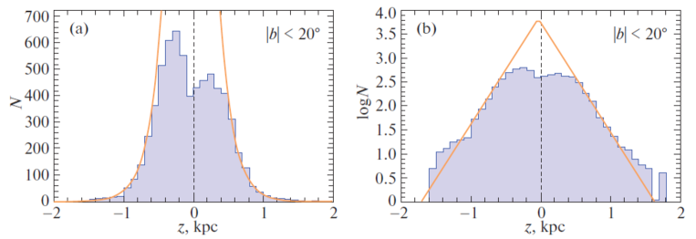
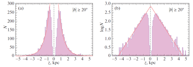
Figures 1 and 2 present histograms of the distribution for the low- and high-latitude HSDs, respectively. Note the difference in the sizes of the horizontal axes in these figures. A deficit of stars near is seen in the figures. In Fig. 2 this dip is largely due to the applied condition , while the conditions for the selection of candidate stars in the catalogue by Geier et al. (2019) are responsible for the “cut-off” top of the distribution in Fig. 1.
| Parameters | ||||
|---|---|---|---|---|
| 15% | 30% | 15% | 30% | |
| 2938 | 3761 | 2176 | 2920 | |
| kpc | 0.96 | 0.97 | 0.98 | 0.96 |
| kpc | 0.16 | 0.17 | 0.57 | 0.56 |
| km s-1 | ||||
| km s-1 | ||||
| km s-1 | ||||
is the number of stars used, is the mean distance of the sample of stars.
| Parameters | kpc | kpc | kpc | kpc |
|---|---|---|---|---|
| 2499 | 1971 | 1193 | 1114 | |
| kpc | 0.82 | 0.99 | 1.04 | 1.18 |
| kpc | 0.10 | 0.29 | 0.49 | 0.81 |
| km s-1 | ||||
| km s-1 | ||||
| km s-1 | ||||
| km s-1 kpc-1 | ||||
| km s-1 kpc-2 | ||||
| km s-1 | ||||
| km s-1 | ||||
| km s-1 | ||||
| km s-1 | ||||
is the number of stars used, is the mean distance of the sample of stars.
Estimating the Surface Density
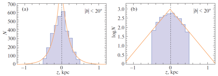
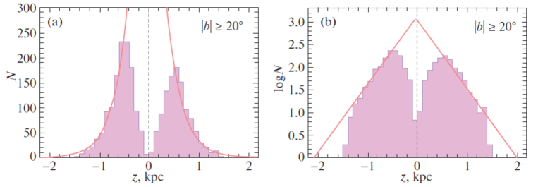
A complete stellar sample is required to estimate the surface density. According to the estimates by Geier et al. (2019), except for the narrow region near the Galactic plane, the catalogue of HSDs is complete to a distance of 1.5 kpc, which we take as the completeness boundary. Thus, in this section we consider the low- and high-latitude HSDs selected under the condition kpc. The results of their analysis are presented in Tables 2 and 3 as well as in Figs. 3 and 4.
As can be seen from Table 2, the scale height remains almost constant for the low-latitude HSDs under various sample production conditions. In contrast, for the high-latitude HSDs h depends strongly on the constraints used. We can see that the moderate kpc is consistent with the results of the analysis of white dwarfs (Vennes et al. 2002) and planetary nebulae (Bobylev and Bajkova 2017b).
As can be seen from Table 3, the third axis in all ellipsoids is close to the direction to the Galactic Pole. Therefore, in Eq. (17) we may set . This is apparently the only way of estimating the vertical velocity, because in our case we have no information about the radial velocities and, therefore, we cannot directly calculate the space velocities and
Let us make an estimate for the mean given in Table 3. We see that kpc for the low-latitude HSDs, which is of no real interest for the estimate of due to the small From the high-latitude HSDs at and kpc we find kpc-2.
For comparison, we can give some values of the surface density obtained by other authors. Korchagin et al. (2003) found kpc-2 for kpc based on a sample of 1500 red giants from the Hipparcos catalogue (1997). Based on giants from the Hipparcos catalogue (1997), Holmberg and Flynn (2004) estimated the local density of the visible matter, kpc-2, and the entire gravitating matter, including the dark matter disk and halo, kpc-2, for 1.1 kpc. Based on 16 000 G dwarfs from the SEGUE catalogue (Yanny et al. 2007), Bovy and Rix (2013) estimated the local stellar density, kpc-2, and the density of the entire gravitating matter, kpc-2, for 1.1 kpc. Based on stars from the TGAS catalogue (Tycho–Gaia Astrometric Solution, Prusti et al. 2016; Lindegren et al. 2016), Kipper et al. (2018) found kpc-2 for kpc.
Dependence of Kinematic Parameters on
In this section we consider the dependence of some kinematic parameters on the coordinate based on a complete sample of HSDs. For this purpose, we used a sample of HSDs with errors ¡30%, which we divided into four nonoverlapping parts, depending on The results are presented in Table 4. Equations (1)–(2) were solved with five unknowns: and . Here we did not divide the stars into low- and high-latitude ones. We see good agreement between the parameters of the residual velocity ellipsoid inferred from both high-latitude HSDs (Table 3) and HSDs with large (Table 4). In particular, km s-1 at large Thus, we correctly estimated the surface density
Based on the data from this table, we estimated the gradient of the circular rotation velocity as a function of km s-1 kpc-1, by fitting a linear trend from four measurements. For comparison, based on a sample of metal-poor stars in the solar neighborhood, Chiba and Beers (2000) obtained the following estimates of such gradients: km s-1 kpc-1 for thin-disk stars with a velocity ellipsoid km s-1 and km s-1 kpc-1 for halo stars with a highly elongated velocity ellipsoid km s-1.
CONCLUSIONS
We studied the kinematics of hot dim stars from the catalogue by Geier et al. (2019). These are 39 800 HSD candidates selected by them from the Gaia DR2 catalogue using data from several multiband photometric sky surveys. In this paper we analyzed more than 12 500 proper motions of stars with relative trigonometric parallax errors less than 30%. Thus,we investigated a huge set of present-day highly accurate data that is of great value for a statistical analysis.
The stars were divided into two parts, depending on the Galactic latitude, into low-latitude () and high-latitude () samples. Such a breakdown is needed to construct the histograms in a wide range and to determine the parameters of the exponential density distribution from them. These two samples were shown to have completely different kinematics. We determined the Galactic rotation parameters from relatively more distant objects whose parallax errors do not exceed 30%. In that case, at least the first derivative of the angular velocity of Galactic rotation is determined quite reliably. In contrast, for the subsequent determination of the residual velocity ellipsoid parameters we already use more reliable data, objects with trigonometric parallax errors no greater than 15%.
For example, the sample of low-latitude HSDs rotates around the Galactic center with a linear velocity km s-1. This suggests that they belong to the Galactic thin disk. They lag behind the local standard of rest by km s-1 due to the asymmetric drift. The high-latitude HSDs rotate with a considerably lower velocity, km s-1, which is more typical for the thick disk. Their lagging behind the local standard of rest is km s-1.
A joint analysis of the entire sample of 12 515 stars with parallax errors less than 30% revealed a positive rotation around the x axis differing significantly from zero with an angular velocity km s-1 kpc-1. Expressed in different units, given the mean distance of the sample stars, this angular velocity is 3 mas yr-1. The latter value is consistent with the estimates by Lindblad et al. (2018) for the residual rotation of the Gaia DR2 reference frame relative to the inertial reference frame.
Based on a sample of 4181 low-latitude HSDs with parallax errors less than 15%, we determined the following principal semiaxes of the residual velocity ellipsoid: km s-1. To within 3–4∘, the principal axes of this ellipsoid coincide in directions with the axes of the Galactic rectangular coordinate system
Based on a sample of 3584 high-latitude HSDs with parallax errors less than 15%, we found km s-1, with the third axis of this ellipsoid (24) being deflected from the direction to the Galactic Pole by Such a deflection is also confirmed by the direction of the second axis with the error having been estimated here along each axis independently.
We studied two samples of HSDs that are complete within kpc. The following vertical disk scale heights were derived: pc and pc from the low- and high-latitude HSDs, respectively. Here, we obtained a new estimate of the local stellar density kpc-2 for kpc from the high-latitude HSDs.
Based on a sample that is complete with errors ¡30%, we traced the evolution of the kinematic parameters as a function of the coordinate We estimated the gradient of the circular rotation velocity along km s-1 kpc-1.
All of the above results lead us to conclude that the low- and high-latitude HSDs exhibit the kinematics of the thin and thick disks, respectively. This suggests that most of the low-latitude HSDs “inherited” the kinematic properties of relatively young massive precursor stars. The high-latitude HSDs are less homogeneous kinematically; their properties depend strongly on the positions above the Galactic plane and the heliocentric distance. Kinematically more “heated” objects that have already receded quite far from the Galactic plane are apparently their precursors.
ACKNOWLEDGMENTS
We are grateful to the referees for the useful remarks that contributed to an improvement of the paper.
REFERENCES
1. M. Altmann, H. Edelmann, and K. S. de Boer, Astron. Astrophys. 414, 181 (2004).
2. B. Anguiano, S. R. Majewski, K. C. Freeman, A. W. Mitschang, and M. C. Smith, Mon. Not. R. Astron. Soc. 474, 854 (2018).
3. F. Arenou, X. Luri, C. Babusiaux, C. Fabricius, A. Helmi, T. Muraveva, A. C. Robin, F. Spoto, et al. (Gaia Collab.), Astron. Astrophys. 616, 17 (2018).
4. V. V. Bobylev, Astron. Lett. 36, 634 (2010).
5. V. V. Bobylev, Astron. Lett. 39, 819 (2013).
6. V. V. Bobylev and A. T. Bajkova, Astron. Lett. 40, 389 (2014).
7. V. V. Bobylev and A. T. Bajkova, Astron. Lett. 42, 1 (2016).
8. V. V. Bobylev and A. T. Bajkova, Astron. Lett. 43, 452 (2017a).
9. V. V. Bobylev and A. T. Bajkova, Astron. Lett. 43, 304 (2017b).
10. V. V. Bobylev and A. T. Bajkova, Astron. Lett. 45, 208 (2019).
11. C. Bonatto, L. O. Kerber, E. Bica, and B. X. Santiago, Astron. Astrophys. 446, 121 (2006).
12. J. Bovy and H.-W. Rix, Astrophys. J. 779, 115 (2013).
13. A. G. A. Brown, A. Vallenari, T. Prusti, J. de Bruijne, F. Mignard, R. Drimmel, et al. (Gaia Collab.), Astron. Astrophys. 595, 2 (2016).
14. A. G. A. Brown, A. Vallenari, T. Prusti, de Bruijne, C. Babusiaux, C. A. L. Bailer-Jones, M. Biermann, D.W. Evans, et al. (Gaia Collab.), Astron. Astrophys. 616, 1 (2018).
15. Y. Bu, Z. Lei, G. Zhao, J. Bu, and J. Pan, Astrophys. J. Suppl. Ser. 233, 2 (2017).
16. T. Camarillo, M. Varun, M. Tyler, and R. Bharat, Publ. Astron. Soc. Pacif. 130, 4101 (2018).
17. M. Chiba and T. C. Beers, Astron. J. 119, 2843 (2000).
18. G. Fontaine, P. Brassard, S. Charpinet, E. M. Green, S. K. Randall, and V. Van Grootel, Astron. Astrophys. 539, 12 (2012).
19. B. Fuchs, C. Dettbarn, H.-W. Rix, T. C. Beers, D. Bizyaev, H. Brewington, H. Jahreiss, R. Klement, et al., Astron. J. 137, 4149 (2009).
20. S. Geier, S. Nesslinger, U. Heber, N. Przybilla, R. Napiwotzki, and R.-P. Kudritzki, Astron. Astrophys. 464, 299 (2007).
21. S. Geier, T. Kupfer, U. Heber, V. Schaffenroth, B. N. Barlow, R. H. Oestensen, S. J. O’Toole, E. Ziegerer, et al., Astron. Astrophys. 577, 26 (2015).
22. S. Geier, R. Raddi, N. P. Gentile Fusillo, and T. R. Marsh, Astron. Astrophys. 621, 38 (2019).
23. J. L. Greenstein and A. I. Sargent, Astrophys. J. Suppl. 28, 157 (1974).
24. R. de Grijs and G. Bono, Astrophys. J. Suppl. Ser. 232, 22 (2017).
25. Z. Han, Ph. Podsiadlowski, and A. E. Lynas-Gray, Mon. Not. R. Astron. Soc. 380, 1098 (2007).
26. The HIPPARCOS and Tycho Catalogues, ESA SP–1200 (1997).
27. J. Holmberg and C. Flynn, Mon. Not. R. Astron. Soc. 352, 440 (2004).
28. M. L. Humason and F. Zwicky, Astrophys. J. 105, 85 (1947).
29. R. Kipper, E. Tempel, and P. Tenjes, Mon. Not. R. Astron. Soc. 473, 2188 (2018).
30. V. I. Korchagin, T. M. Girard, T. V. Borkova, D. I. Dinescu, and W. F. van Altena, Astron. J. 126, 2896 (2003).
31. T. Kupfer, S. Geier, U. Heber, R. H. Ostensen, B. N. Barlow, P. F. L. Maxted, C. Heuser, V. Schaffenroth, and B. T. Gansicke, Astron. Astrophys. 576, 44 (2015).
32. M. Latour, P. Chayer, E. M. Green, A. Irrgang, and G. Fontaine, Astron. Astrophys. 609, 89 (2018).
33. Z. Lei, G. Zhao, A. Zeng, L. Shen, Z. Lan, D. Jiang, and Z. Han, Mon. Not. R. Astron. Soc. 463, 3449 (2016).
34. L. Lindegren, U. Lammers, U. Bastian, J. Hernandez, S. Klioner, D. Hobbs, A. Bombrun, D. Michalik, et al., Astron. Astrophys. 595, 4 (2016).
35. L. Lindegren, J. Hernandez, A. Bombrun, S. Klioner, U. Bastian, M. Ramos-Lerate, A. de Torres, H. Steidelmuller, et al. (Gaia Collab.), Astron. Astrophys. 616, 2 (2018).
36. M. López-Corredoira, H. Abedi, F. Garzón, and F. Figueras, Astron. Astrophys. 572, 101 (2014).
37. M. Miyamoto and Z. Zhu, Astron. J. 115, 1483 (1998).
38. K.F. Ogorodnikov, Dynamics of stellar systems (Oxford: Pergamon, ed. Beer, A. 1965).
39. E.-M. Pauli, R. Napiwotzki, U. Heber, M. Altmann, and M. Odenkirchen, Astron. Astrophys. 447, 173 (2006).
40. T. Prusti, J.H. J. de Bruijne, A. G. A. Brown, A. Vallenari, C. Babusiaux, C. A. L. Bailer-Jones, U. Bastian, M. Biermann, et al. (Gaia Collab.), Astron. Astrophys. 595, 1 (2016).
41. S. K. Randall, A. Calamida, G. Fontaine, M. Monelli, G. Bono, M. L. Alonso, V. Van Groote, P. Brassard, et al., Astron. Astrophys. 589, 1 (2016).
42. A. S. Rastorguev, M. V. Zabolotskikh, A. K. Dambis, N. D. Utkin, V. V. Bobylev, and A. T. Bajkova, Astrophys. Bull. 72, 122 (2017).
43. A. G. Riess, S. Casertano, W. Yuan, L. Macri, B. Bucciarelli, M. G. Lattanzi, J. W. MacKenty, J. B. Bowers, et al., Astrophys. J. 861, 126 (2018).
44. M. Romero-Gómez, C. Mateu, L. Aguilar, F. Figueras, and A. Castro-Ginard, arXiv: 1812.07576 (2018).
45. N. Rowell and N. C. Hambly, Mon. Not. R. Astron. Soc. 417, 93 (2011).
46. R. Schönrich, J. Binney, and W. Dehnen, Mon. Not. R. Astron. Soc. 403, 1829 (2010).
47. L. Spitzer, Astrophys. J. 95, 329 (1942).
48. K. G. Stassun and G. Torres, Astrophys. J. 862, 61 (2018).
49. A. S. Tsvetkov and F. A. Amosov, Astron. Lett. 45, 462 (2019).
50. J. P. Vallée, Astrophys. Space Sci. 362, 79 (2017).
51. S. Vennes, R. J. Smith, B. J. Boyle, S. M. Croom, A. Kawka, T. Shanks, L. Miller, and N. Loaring, Mon. Not. R. Astron. Soc. 335, 673 (2002).
52. V. V. Vityazev, A. S. Tsvetkov, V. V. Bobylev, and A. T. Bajkova, Astrofizika 60, 503 (2017).
53. J. Vos, P. Németh, M. Vuc̆ković, R. Ostensen, and S. Parsons, Mon. Not. R. Astron. Soc. 473, 693 (2018).
54. L. N. Yalyalieva, A. A. Chemel’, E. V. Glushkova, A. K. Dambis, and A. D. Klinichev, Astrophys. Bull. 73, 335 (2018).
55. B. Yanny, C. Rockosi, H. J. Newberg, G. R. Knapp, J. K. Adelman-McCarthy, B. Alcorn, S. Allam, C. A. Prieto, et al., Astron. J. 137, 4377 (2009).
56. J. C. Zinn, M. H. Pinsonneault, D. Huber, and D. Stello, arXiv: 1805.02650 (2018).