Discrete Laplacian in a half-space with a periodic surface potential I ​: Resolvent expansions, scattering matrix, and wave operators

Abstract

We present a detailed study of the scattering system given by the Neumann Laplacian on the discrete half-space perturbed by a periodic potential at the boundary. We derive asymptotic resolvent expansions at thresholds and eigenvalues, we prove the continuity of the scattering matrix, and we establish new formulas for the wave operators. Along the way, our analysis puts into evidence a surprising relation between some properties of the potential, like the parity of its period, and the behaviour of the integral kernel of the wave operators.

1. Graduate school of mathematics, Nagoya University, Chikusa-ku,
   Nagoya 464-8602, Japan

2. Facultad de Matemáticas, Pontificia Universidad Católica de Chile,
   Av. Vicuña Mackenna 4860, Santiago, Chile

3. E-mails: nguyen.ha.song@b.mbox.nagoya-u.ac.jp, richard@math.nagoya-u.ac.jp,
   E-mails: rtiedra@mat.uc.cl

2010 Mathematics Subject Classification: 81Q10, 47A40

Keywords: resolvent expansions, scattering matrix, wave operators, discrete Laplacian, thresholds.

1 Introduction and main results

For the last 20 years, Schrödinger operators with potentials supported on lower dimensional subspaces have been the subject of an intensive study motivated by both physical applications and mathematical interest, see for example [2, 3, 4, 6, 7, 8, 13] and references therein. These systems exhibit properties that are intermediate between the ones of standard scattering systems (with potentials decaying in all space directions) and the ones of bulk systems (with potentials having no specific space decay). A fundamental example of such property, appearing in discrete and in continuous settings, is the presence of surface states propagating along the lower dimensional subspace. Our goal is to present a detailed study of these surface states from a $C^{*}$-algebraic point of view for a two-dimensional system on the discrete lattice. In particular, we plan to establish an index-type theorem relating the surface states to the scattering part of the system, as it was done in various other contexts [1, 9, 21, 24]. However, before any $C^{*}$-algebraic construction and prior to any index theorem, a lot of analysis is needed. This is the subject of this first part of a series of two papers.

The model that we consider is a simple and natural quantum system exhibiting surface states. It is given by a Laplace operator on a discrete half-space, subject to a periodic potential at the boundary. See Figure 1. Despite its simplicity, this model requires a non-trivial analysis, and exhibits some unexpected properties. The model has already been studied, for instance in [2, 3], but our paper contains more extensive results on scattering theory, presented within an up-to-date framework.

Let us now give a description of our principal results. In the Hilbert space $\mathcal{H}:=\ell^{2}(\mathbb{Z}\times\mathbb{N})\cong\ell^{2}(\mathbb{Z})\otimes\ell^{2}(\mathbb{N})$, we consider the free Hamiltonian

$$H_{0}:=\Delta_{\mathbb{Z}}\otimes 1+1\otimes\Delta_{\mathrm{N}},$$

where $\Delta_{\mathbb{Z}}$ is the adjacency operator in $\ell^{2}(\mathbb{Z})$ given by

$$\big{(}\Delta_{\mathbb{Z}}\;\!\varphi\big{)}(x):=\varphi(x+1)+\varphi(x-1),\quad\varphi\in\ell^{2}(\mathbb{Z}),~{}x\in\mathbb{Z},$$

and where $\Delta_{\mathrm{N}}$ is the discrete Neumann adjacency operator in $\ell^{2}(\mathbb{N})$ given by

$$\big{(}\Delta_{\mathrm{N}}\;\!\phi\big{)}(n)=\begin{cases}2^{1/2}\;\!\phi(1)&\hbox{if $n=0$}\\ 2^{1/2}\;\!\phi(0)+\phi(2)&\hbox{if $n=1$}\\ \phi(n+1)+\phi(n-1)&\hbox{if $n\geq 2$,}\end{cases}\quad\phi\in\ell^{2}(\mathbb{N}),~{}n\in\mathbb{N}.$$

As a full Hamiltonian, we consider the operator

$$H:=H_{0}+V,$$

where $V$ is the multiplication operator by a nonzero, periodic, real-valued function with support on $\mathbb{Z}\times\{0\}$. In other words, we assume that there exists a nonzero periodic function $v:\mathbb{Z}\to\mathbb{R}$ of period $N\in\mathbb{N}$, $N\geq 2$, (the potential) such that

$$(H\psi)(x,n)=(H_{0}\psi)(x,n)+\delta_{0,n}\;\!v(x)\;\!\psi(x,0),\quad\psi\in\mathcal{H},~{}x\in\mathbb{Z},~{}n\in\mathbb{N},$$

with $\delta_{0,n}$ the Kronecker delta function. Note that the multiplication operator $V$ associated to the potential $v$ is not a compact perturbation of $H_{0}$.

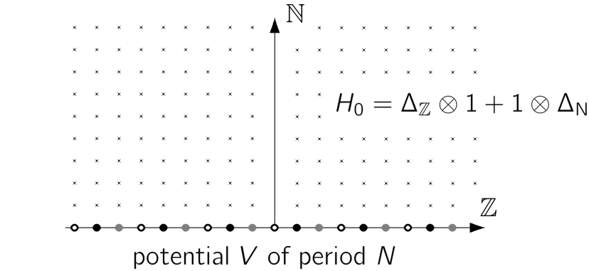
Figure 1: Sketch of the two-dimensional discrete model

Since the operators $H_{0}$ and $H$ are $N$-periodic in the $x$-variable, they can be decomposed using a Bloch-Floquet transformation. Namely, if we set $\mathfrak{h}:=\mathop{\mathrm{L}^{2}}\nolimits\big{(}[0,\pi),\tfrac{\mathrm{d}\omega}{\pi};\mathbb{C}^{N}\big{)}$ and $\mathfrak{H}:=\int_{[0,2\pi]}^{\oplus}\mathfrak{h}\;\!\tfrac{\mathrm{d}\theta}{2\pi}$, then it can be shown that $H_{0}$ and $H$ are unitarily equivalent to the direct integral operators in $\mathfrak{H}$

$$\int_{[0,2\pi]}^{\oplus}H^{\theta}_{0}\;\!\tfrac{\mathrm{d}\theta}{2\pi}\quad\hbox{with}\quad H^{\theta}_{0}:=2\cos(\Omega)+A^{\theta}$$ (1.1)

and

$$\int_{[0,2\pi]}^{\oplus}H^{\theta}\;\!\tfrac{\mathrm{d}\theta}{2\pi}\quad\hbox{with}\quad H^{\theta}:=2\cos(\Omega)+A^{\theta}+\mathop{\mathrm{diag}}\nolimits(v)P_{0}$$ (1.2)

where $\cos(\Omega)$ is the multiplication operator by the function $\omega\to\cos(\omega)$ in $\mathfrak{h}$, $A^{\theta}$ is the $N\times N$ hermitian matrix

$$A^{\theta}:=\left(\begin{smallmatrix}0&1&0&\cdots&0&\mathop{\mathrm{e}}\nolimits^{-i\theta}\\ 1&0&1&\ddots&&0\\ 0&1&\ddots&\ddots&\ddots&\vdots\\ \vdots&\ddots&\ddots&\ddots&1&0\\ 0&&\ddots&1&0&1\\ \mathop{\mathrm{e}}\nolimits^{i\theta}&0&\cdots&0&1&0\end{smallmatrix}\right),$$ (1.3)

and

$$\big{(}\mathop{\mathrm{diag}}\nolimits(v)\;\!\mathfrak{f}(\theta,\;\!\cdot\;\!)\big{)}_{j}:=v(j)\;\!\mathfrak{f}_{j}(\theta,\;\!\cdot\;\!)\quad\hbox{and}\quad\big{(}P_{0}\;\!\mathfrak{f}(\theta,\;\!\cdot\;\!)\big{)}_{j}:=\int_{0}^{\pi}\mathfrak{f}_{j}(\theta,\omega)\tfrac{\mathrm{d}\omega}{\pi}$$ (1.4)

for $\mathfrak{f}\in\mathfrak{H}$, $j\in\{1,\dots,N\}$ and a.e. $\theta\in[0,2\pi]$. The main interest of the above representation is that for each fixed $\theta$ the operator $\mathop{\mathrm{diag}}\nolimits(v)P_{0}$ is a finite rank perturbation of the operator $H_{0}^{\theta}$.

Remark 1.1.

A direct inspection shows that the matrix $A^{\theta}$ has eigenvalues

$$\lambda_{j}^{\theta}:=2\cos\left(\tfrac{\theta+2\pi\;\!j}{N}\right),\quad j\in\{1,\dots,N\},$$

with corresponding eigenvectors $\xi_{j}^{\theta}\in\mathbb{C}^{N}$ having components $\big{(}\xi_{j}^{\theta}\big{)}_{k}:=\mathop{\mathrm{e}}\nolimits^{i(\theta+2\pi j)k/N}$, $j,k\in\{1,\dots,N\}$. Using the notation $\mathcal{P}_{j}^{\theta}$ for the orthogonal projection associated to $\xi_{j}^{\theta}$, we thus can write $A^{\theta}$ as $A^{\theta}=\sum_{j=1}^{N}\lambda_{j}^{\theta}\;\!\mathcal{P}_{j}^{\theta}$.

Due to the unitary equivalences, the analysis of the pair of operators $(H,H_{0})$ in the Hilbert space $\mathcal{H}$ reduces to the analysis of the family of pairs of operators $(H^{\theta},H^{\theta}_{0})$ indexed by the quasi-momentum $\theta\in[0,2\pi]$ in the Hilbert space $\mathfrak{h}$. Therefore, from now on we present our results for the operators $H^{\theta}$ and $H^{\theta}_{0}$ at fixed $\theta$, and come back to the initial pair $(H,H_{0})$ later on.

Constructing a spectral representation of $H^{\theta}_{0}$ is fairly direct. Intuitively, it amounts to diagonalising the matrix $A^{\theta}$ and linearising the function $\cos$. More precisely, first we define for $\theta\in[0,2\pi]$ and $j\in\{1,\dots,N\}$ the sets

$$I_{j}^{\theta}:=(\lambda_{j}^{\theta}-2,\lambda_{j}^{\theta}+2)\quad\hbox{and}\quad I^{\theta}:=\cup_{j=1}^{N}I^{\theta}_{j}.$$

Next, we define the fiber Hilbert spaces

$$\mathscr{H}^{\theta}(\lambda):=\mathop{\mathrm{span}}\nolimits\big{\{}\mathcal{P}^{\theta}_{j}\mathbb{C}^{N}\mid\hbox{$j\in\{1,\dots,N\}$ such that $\lambda\in I_{j}^{\theta}$}\big{\}}\subset\mathbb{C}^{N},\quad\lambda\in I^{\theta},$$

and the corresponding direct integral Hilbert space

$$\mathscr{H}^{\theta}:=\int_{I^{\theta}}^{\oplus}\mathscr{H}^{\theta}(\lambda)\;\!\mathrm{d}\lambda.$$

Then, it is easily verified that the operator $\mathscr{F}^{\theta}:\mathfrak{h}\to\mathscr{H}^{\theta}$ defined by

$$\big{(}\mathscr{F}^{\theta}g\big{)}(\lambda):=\pi^{-1/2}\sum_{\{j\mid\lambda\in I_{j}^{\theta}\}}\big{(}4-(\lambda-\lambda_{j}^{\theta})^{2}\big{)}^{-1/4}\;\!\mathcal{P}^{\theta}_{j}g\Big{(}\arccos\Big{(}\tfrac{\lambda-\lambda_{j}^{\theta}}{2}\Big{)}\Big{)},\quad g\in\mathfrak{h},~{}\hbox{a.e. $\lambda\in I^{\theta}$,}$$

is unitary, with adjoint $(\mathscr{F}^{\theta})^{*}:\mathscr{H}^{\theta}\to\mathfrak{h}$ given by

$$\big{(}(\mathscr{F}^{\theta})^{*}\zeta\big{)}(\omega):=\big{(}2\pi\sin(\omega)\big{)}^{1/2}\sum_{j=1}^{N}\mathcal{P}_{j}^{\theta}\zeta\big{(}2\cos(\omega)+\lambda_{j}^{\theta}\big{)},\quad\zeta\in\mathscr{H}^{\theta},~{}\hbox{a.e. $\omega\in[0,\pi)$.}$$ (1.5)

In addition, $\mathscr{F}^{\theta}$ diagonalises the Hamiltonian $H_{0}^{\theta}$. Namely, for all $\zeta\in\mathscr{H}^{\theta}$ and a.e. $\lambda\in I^{\theta}$ one has

$$\big{(}\mathscr{F}^{\theta}H_{0}^{\theta}\;\!(\mathscr{F}^{\theta})^{*}\zeta\big{)}(\lambda)=\lambda\;\!\zeta(\lambda)=\big{(}X^{\theta}\zeta\big{)}(\lambda),$$

with $X^{\theta}$ the (bounded) operator of multiplication by the variable in $\mathscr{H}^{\theta}$. As a consequence, one infers that $H_{0}^{\theta}$ has purely absolutely continuous spectrum equal to

$$\textstyle\sigma(H_{0}^{\theta})=\overline{\mathop{\mathrm{Ran}}\nolimits(X^{\theta})}=\overline{I^{\theta}}=\big{[}(\min_{j}\lambda_{j}^{\theta})-2,(\max_{j}\lambda_{j}^{\theta})+2\big{]}\subset[-4,4]$$ (1.6)

and also that $\sigma(H_{0})=\overline{\bigcup_{\theta\in[0,2\pi]}\sigma(H_{0}^{\theta})}=[-4,4]$. Moreover, the spectral representation of $H^{\theta}_{0}$ naturally leads to the notion of thresholds of $H^{\theta}_{0}$; namely, the set $\mathcal{T}^{\theta}$ of real values where the spectrum of $H^{\theta}_{0}$ presents a change of multiplicity:

$$\mathcal{T}^{\theta}:=\big{\{}\lambda_{j}^{\theta}\pm 2\mid j\in\{1,\dots,N\}\big{\}}.$$ (1.7)

The next step is the analysis of the operator $H^{\theta}$, which is detailed in Section 3. In short, we determine the spectral properties of $H^{\theta}$ and we establish resolvent expansions for $H^{\theta}$ near the thresholds. Based on the resolvent expansions, we also derive various properties of the scattering operator for the pair $(H^{\theta},H^{\theta}_{0})$.

Regarding the spectral analysis, the main result is a necessary and sufficient condition for the existence of eigenvalues of $H^{\theta}$. To state it, we use standard notations borrowed from [14, 26]. First of all, we decompose the matrix $\mathop{\mathrm{diag}}\nolimits(v):=(v(1),\dots,v(N))$ as the product $\mathop{\mathrm{diag}}\nolimits(v)=\mathfrak{u}\mathfrak{v}^{2}$, where $\mathfrak{v}:=|\mathop{\mathrm{diag}}\nolimits(v)|^{1/2}$ and $\mathfrak{u}:=\mathop{\mathrm{sgn}}\nolimits\big{(}\mathop{\mathrm{diag}}\nolimits(v)\big{)}$ is the diagonal matrix with components

$$\mathfrak{u}_{jj}=\mathop{\mathrm{sgn}}\nolimits\big{(}\mathop{\mathrm{diag}}\nolimits(v)\big{)}_{jj}=\begin{cases}+1&\hbox{if $v(j)\geq 0$}\\ -1&\hbox{if $v(j)<0$,}\end{cases}\quad j\in\{1,\dots,N\}.$$

We also introduce the functions

$$\beta_{j}^{\theta}(z):=\big{|}(z-\lambda_{j}^{\theta})^{2}-4\big{|}^{1/4},\quad j\in\{1,\dots,N\},~{}\theta\in[0,2\pi],~{}z\in\mathbb{C}.$$ (1.8)

The spectral result for $H^{\theta}$ then reads as follows (recall Remark 2.1 for the definitions of $\lambda_{j}^{\theta}$ and $\mathcal{P}_{j}^{\theta}$):

Proposition 1.2.

A value $\lambda\in\mathbb{R}\setminus\mathcal{T}^{\theta}$ is an eigenvalue of $H^{\theta}$ if and only if

$${\mathcal{K}}:=\ker\left(\mathfrak{u}+\sum_{\{j\mid\lambda<\lambda_{j}^{\theta}-2\}}\tfrac{\mathfrak{v}\;\!\mathcal{P}_{j}^{\theta}\mathfrak{v}}{\beta_{j}^{\theta}(\lambda)^{2}}-\sum_{\{j\mid\lambda>\lambda_{j}^{\theta}+2\}}\tfrac{\mathfrak{v}\;\!\mathcal{P}_{j}^{\theta}\mathfrak{v}}{\beta_{j}^{\theta}(\lambda)^{2}}\right)\bigcap\left(\cap_{\{j\mid\lambda\in I^{\theta}_{j}\}}\ker\big{(}\mathcal{P}_{j}^{\theta}\mathfrak{v}\big{)}\right)\neq\{0\},$$

in which case the multiplicity of $\lambda$ equals the dimension of $\mathcal{K}$.

Next, we use a general approach for resolvent expansions [14, 22] to derive detailed asymptotic resolvent expansions for $H^{\theta}$. For that purpose, we introduce the bounded operator $G:\mathfrak{h}\to\mathbb{C}^{N}$ given by

$$(Gg)_{j}:=\mathfrak{v}_{jj}\int_{0}^{\pi}g_{j}(\omega)\;\!\tfrac{\mathrm{d}\omega}{\pi}=|v(j)|^{1/2}\int_{0}^{\pi}g_{j}(\omega)\;\!\tfrac{\mathrm{d}\omega}{\pi},\quad g\in\mathfrak{h},~{}j\in\{1,\dots,N\}.$$ (1.9)

Then, the results we obtain about the resolvent of $H^{\theta}$ are formulated as asymptotic expansions for the operator

$$M^{\theta}(\lambda+i\varepsilon):=\big{(}\mathfrak{u}+G(H_{0}^{\theta}-\lambda-i\varepsilon)^{-1}G^{*}\big{)}^{-1},\quad\lambda,\varepsilon\in\mathbb{R},~{}\varepsilon\neq 0,$$ (1.10)

as $\varepsilon\to 0$. They are expressed in terms of projections $S_{0},S_{1},S_{2}$ in $\mathbb{C}^{N}$ of decreasing range, with the most singular divergences of the expansions taking place in the ranges of the projections of higher indices (the greater the divergence, the smaller the subspace where it takes place, see Proposition 3.4 for details). The asymptotic expansions are valid for any point $\lambda$ in the spectrum of $H^{\theta}$. That is, when $\lambda$ is a threshold of $H^{\theta}$, when $\lambda$ is an eigenvalue of $H^{\theta}$, and when $\lambda$ is neither a threshold, nor an eigenvalue of $H^{\theta}$. The expansions imply as a by-product the finiteness of point spectrum of $H^{\theta}$, see Remark 3.6.

Once obtained the asymptotic expansions for the operator (1.10), we can establish our next main result, which is the the continuity of the scattering matrix. The previous works on the two-dimensional discrete model studied here have discussed the problem of the existence and the completeness of the wave operators. Such results lead to the existence and the unitarity of the scattering operator, but do not say anything about the continuity of the scattering matrix. And this continuity property will be needed in our second paper in order to apply the $C^{*}$-algebraic technics leading to the index theorem.

To formulate the continuity property of the scattering matrix, we first note that the wave operators

$$W_{\pm}^{\theta}:=\operatorname*{s\hskip 0.1pt-\hskip 0.1ptlim}_{t\to\pm\infty}\mathop{\mathrm{e}}\nolimits^{itH^{\theta}}\mathop{\mathrm{e}}\nolimits^{-itH^{\theta}_{0}}$$

exist and are complete since the difference $H^{\theta}-H^{\theta}_{0}$ is a finite rank operator, see [16, Thm. X.4.4]. As a consequence, the scattering operator $S^{\theta}:=(W_{+}^{\theta})^{*}W_{-}^{\theta}$ is a unitary operator in $\mathfrak{h}$ commuting with $H^{\theta}_{0}$. Therefore, $S^{\theta}$ is decomposable in the spectral representation of $H^{\theta}_{0}$, that is,

$$\big{(}\mathscr{F}^{\theta}S^{\theta}(\mathscr{F}^{\theta})^{*}h\big{)}(\lambda)=S^{\theta}(\lambda)h(\lambda),\quad\hbox{$h\in\mathscr{H}^{\theta}$, a.e. $\lambda\in\sigma(H^{\theta}_{0})$,}$$

where $S^{\theta}(\lambda)$ (the scattering matrix at energy $\lambda$) is a unitary operator in $\mathscr{H}^{\theta}(\lambda)$. To give an explicit formula for $S^{\theta}(\lambda)$, Proposition 1.2 and the asymptotic expansions play a key role. Indeed, it follows from them that the limit

$$M^{\theta}(\lambda+i0):=\lim_{\varepsilon\searrow 0}\big{(}\mathfrak{u}+G(H_{0}^{\theta}-\lambda-i\varepsilon)^{-1}G^{*}\big{)}^{-1}$$

exists and belongs to $\mathscr{B}(\mathbb{C}^{N})$ for each $\lambda\in\sigma(H_{0}^{\theta})\setminus\big{(}\mathcal{T}^{\theta}\cup\sigma_{\rm p}(H^{\theta})\big{)}$, where $\sigma_{\rm p}(H^{\theta})$ is the point spectrum of $H^{\theta}$. And then, a computation using stationary formulas [26, Sec. 2.8] shows for $\lambda\in(I^{\theta}_{j}\cap I^{\theta}_{j^{\prime}})\setminus\big{(}\mathcal{T}^{\theta}\cup\sigma_{\rm p}(H^{\theta})\big{)}$ and $j,j^{\prime}\in\{1,\dots,N\}$ that the channel scattering matrix $S^{\theta}(\lambda)_{jj^{\prime}}:=\mathcal{P}^{\theta}_{j}S^{\theta}(\lambda)\mathcal{P}^{\theta}_{j^{\prime}}$ is given by

$$S^{\theta}(\lambda)_{jj^{\prime}}=\delta_{jj^{\prime}}-2i\;\!\beta_{j}^{\theta}(\lambda)^{-1}\mathcal{P}_{j}^{\theta}\mathfrak{v}\;\!M^{\theta}(\lambda+i0)\mathfrak{v}\;\!\mathcal{P}_{j^{\prime}}^{\theta}\;\!\beta_{j^{\prime}}^{\theta}(\lambda)^{-1},$$ (1.11)

where the operator $\delta_{jj^{\prime}}\in\mathscr{B}\big{(}\mathcal{P}_{j^{\prime}}^{\theta}\;\!\mathbb{C}^{N};\mathcal{P}_{j}^{\theta}\;\!\mathbb{C}^{N}\big{)}$ is defined by $\delta_{jj^{\prime}}:=1$ if $j=j^{\prime}$ and $\delta_{jj^{\prime}}:=0$ otherwise. Now, an explicit formula for $G(H_{0}^{\theta}-\lambda-i0)^{-1}G^{*}$ (see (3.3)) implies the continuity of the map

$$(I^{\theta}_{j}\cap I^{\theta}_{j^{\prime}})\setminus\big{(}\mathcal{T}^{\theta}\cup\sigma_{\rm p}(H^{\theta})\big{)}\ni\lambda\mapsto S^{\theta}(\lambda)_{jj^{\prime}}\in\mathscr{B}\big{(}\mathcal{P}_{j^{\prime}}^{\theta}\mathbb{C}^{N};\mathcal{P}_{j}^{\theta}\mathbb{C}^{N}\big{)}.$$

Therefore, in order to completely establish the continuity of the channel scattering matrices $S^{\theta}(\lambda)_{jj^{\prime}}$, what remains is to describe the behaviour of $S^{\theta}(\lambda)_{jj^{\prime}}$ as $\lambda\to\lambda_{\star}\in\mathcal{T}^{\theta}\cup\sigma_{\rm p}(H^{\theta})$. We consider separately the behaviour of $S^{\theta}(\lambda)_{jj^{\prime}}$ at thresholds and at embedded eigenvalues, starting with the thresholds. For that purpose, we first observe that for each $\lambda\in\mathcal{T}^{\theta}$, a channel can already be open at the energy $\lambda$ (in which case one has to show the existence and the equality of the limits from the right and from the left), it can open at the energy $\lambda$ (in which case one only has to show the existence of the limit from the right), or it can close at the energy $\lambda$ (in which case one only has to show the existence of the limit from the left). Therefore, we fix $\lambda\in\mathcal{T}^{\theta}$, and consider the matrix $S^{\theta}(\lambda+\varepsilon)_{jj^{\prime}}$ for suitable $\varepsilon\in\mathbb{R}$. In this setting, our continuity result can be stated as (see Theorem 3.9 for a more general statement including the values of the limits):

Theorem 1.3.

Let $\lambda\in\mathcal{T}^{\theta}$, take $\varepsilon\in\mathbb{R}$ with $|\varepsilon|$ small enough, and let $j,j^{\prime}\in\{1,\dots,N\}$.

1. If $\lambda\in I^{\theta}_{j}\cap I^{\theta}_{j^{\prime}}$, then the limit $\lim_{\varepsilon\to 0}S^{\theta}(\lambda+\varepsilon)_{jj^{\prime}}$ exists.

2. If $\lambda\in\overline{I^{\theta}_{j}}\cap\overline{I^{\theta}_{j^{\prime}}}$ and $\lambda+\varepsilon\in I^{\theta}_{j}\cap I^{\theta}_{j^{\prime}}$ for $\varepsilon>0$ small enough, then the limit $\lim_{\varepsilon\searrow 0}S^{\theta}(\lambda+\varepsilon)_{jj^{\prime}}$ exists.

3. If $\lambda\in\overline{I^{\theta}_{j}}\cap\overline{I^{\theta}_{j^{\prime}}}$ and $\lambda-\varepsilon\in I^{\theta}_{j}\cap I^{\theta}_{j^{\prime}}$ for $\varepsilon>0$ small enough, then the limit $\lim_{\varepsilon\searrow 0}S^{\theta}(\lambda-\varepsilon)_{jj^{\prime}}$ exists.

We also establish the continuity of the scattering matrix at embedded eigenvalues not located at thresholds, see Theorem 3.10 for more details:

Theorem 1.4.

Let $\lambda\in\sigma_{\rm p}(H^{\theta})\setminus\mathcal{T}^{\theta}$, take $\varepsilon\in\mathbb{R}$ with $|\varepsilon|>0$ small enough, and let $j,j^{\prime}\in\{1,\dots,N\}$. Then, if $\lambda\in I^{\theta}_{j}\cap I^{\theta}_{j^{\prime}}$, the limit $\lim_{\varepsilon\to 0}S^{\theta}(\lambda+\varepsilon)_{jj^{\prime}}$ exists.

Our final results concern the wave operator $W_{-}^{\theta}$. By using the spectral representation of $H_{0}^{\theta}$ and a stationary representation formula for $W_{-}^{\theta}$, we can express $W_{-}^{\theta}$ as the sum of two terms. Namely, we obtain for suitable $\xi,\zeta\in\mathscr{H}^{\theta}$

$$\big{\langle}\mathscr{F}^{\theta}(W_{-}^{\theta}-1)(\mathscr{F}^{\theta})^{*}\xi,\zeta\big{\rangle}_{\mathscr{H}^{\theta}}$$

$$=-\pi^{-1/2}\sum_{j=1}^{N}\int_{I^{\theta}_{j}}\lim_{\varepsilon\searrow 0}\left\langle\mathfrak{v}M^{\theta}(\lambda+i\varepsilon)\mathfrak{v}\;\!\gamma_{0}(\mathscr{F}^{\theta})^{*}\delta_{\varepsilon}(X^{\theta}-\lambda)\xi,\int_{I_{j}^{\theta}}\tfrac{\beta_{j}^{\theta}(\mu)^{-1}}{\mu-\lambda+i\varepsilon}\;\!\zeta_{j}(\mu)\;\!\mathrm{d}\mu\right\rangle_{\mathbb{C}^{N}}\mathrm{d}\lambda$$ (1.12)

$$\quad-\pi^{-1/2}\sum_{j=1}^{N}\int\limits_{\sigma(H^{\theta}_{0})\setminus I^{\theta}_{j}}\lim_{\varepsilon\searrow 0}\left\langle\mathfrak{v}M^{\theta}(\lambda+i\varepsilon)\mathfrak{v}\;\!\gamma_{0}(\mathscr{F}^{\theta})^{*}\delta_{\varepsilon}(X^{\theta}-\lambda)\xi,\int_{I_{j}^{\theta}}\tfrac{\beta_{j}^{\theta}(\mu)^{-1}}{\mu-\lambda+i\varepsilon}\;\!\zeta_{j}(\mu)\;\!\mathrm{d}\mu\right\rangle_{\mathbb{C}^{N}}\mathrm{d}\lambda.$$ (1.13)

with $\delta_{\varepsilon}(X^{\theta}-\lambda):=\frac{\pi^{-1}\varepsilon}{(X^{\theta}-\lambda)^{2}+\varepsilon^{2}}$ and $\gamma_{0}:\mathfrak{h}\to\mathbb{C}^{N}$ given by

$$(\gamma_{0}g)_{j}:=\int_{0}^{\pi}g_{j}(\omega)\tfrac{\mathrm{d}\omega}{\pi},\quad g\in\mathfrak{h},~{}j\in\{1,\dots,N\}.$$ (1.14)

The main term (1.12) could be interpreted as an on-shell contribution, while the remainder term (1.13) could be interpreted as an off-shell contribution.

The interest of such a decomposition is that the main term is equal to the product of an explicit operator independent of the potential, and the operator $S^{\theta}-1$. Namely, we show in Section 4.1 that, up to a compact term, the operator corresponding to (1.12) is unitarily equivalent to

$$\tfrac{1}{2}\big{(}1-\tanh(\pi\mathfrak{D})-i\cosh(\pi\mathfrak{D})^{-1}\tanh(\mathfrak{X})\big{)}(S^{\theta}-1),$$ (1.15)

where $\mathfrak{X}$ and $\mathfrak{D}$ are representations of the canonical position and momentum operators in the Hilbert space $\mathfrak{h}$. This formula is obtained by considering the on-shell contribution in a rescaled energy representation whose importance has been revealed in [1, 24] and which was also used explicitly in [12] and implicitly in [19, 20].

The analysis of the remainder term (1.13) is more involved, and depends on the value of $\theta$. When $\theta\neq 0$ or when $\theta=0$ and $N$ is odd, the operator corresponding to (1.13) extends continuously to a compact operator. Since the operator (1.15) is never compact, this shows that the remainder term can indeed be considered small compared to the leading term. On the other hand, when $\theta=0$ and $N$ is even, more analysis is required. In this case, the compacity argument does not work when the energy bands $[-4,0]$ and $[0,4]$ of $H^{0}$ exactly touch, without overlaping, see Remark 4.7. However, if the vectors $\mathfrak{v}\xi_{N}^{0}$ and $\mathfrak{v}\xi^{0}_{N/2}$ are linearly independent (see Remark 2.1 when $\theta=0$ for the definition of the vectors), one can still show that the remainder term is compact. We thus call degenerate case the very exceptional case where $\theta=0$, $N$ is even, and $\mathfrak{v}\xi_{N}^{0}$ and $\mathfrak{v}\xi^{0}_{N/2}$ are linearly dependent. A direct inspection shows that it takes place if and only if the matrix $\mathfrak{v}$ has the very particular form

$$\mathfrak{v}=\left(\begin{smallmatrix}v(1)&&&&0\\ &0&&&\\ &&v(3)&&\\ &&&0&\\ 0&&&&\ddots\\ \end{smallmatrix}\right)\quad\hbox{or}\quad\mathfrak{v}=\left(\begin{smallmatrix}0&&&&0\\ &v(2)&&&\\ &&0&&\\ &&&v(4)&\\ 0&&&&\ddots\\ \end{smallmatrix}\right).$$ (1.16)

In the degenerate case, the remainder term is bounded but not compact. However, in our second paper, we will show that the remainder term can still be considered small compared to the leading term, once suitable $C^{*}$-algebras are introduced.

Summing up what precedes, we get (see Theorem 4.13 for more details):

Theorem 1.5.

For any $\theta\in[0,2\pi]$, one has the equality

$$W_{-}^{\theta}-1=\tfrac{1}{2}\big{(}1-\tanh(\pi\mathfrak{D})-i\cosh(\pi\mathfrak{D})^{-1}\tanh(\mathfrak{X})\big{)}(S^{\theta}-1)+\mathfrak{K}^{\theta},$$

with $\mathfrak{K}^{\theta}$ compact in the nondegenerate cases, and $\mathfrak{K}^{0}$ bounded in the degenerate case.

This type of formula has been obtained for various models having a finite point spectrum: first in [17, 18], and then in various other papers summarised in the review article [21]. Similar formulas have also been independently obtained in [1] and in [12], and some generalisations to the case of an infinite number of eigenvalues can be found in [10, 11].

The final step is to combine the formulas for the wave operators for all quasi-momenta $\theta$ to obtain a new representation formula for the wave operators $W_{\pm}:=\operatorname*{s\hskip 0.1pt-\hskip 0.1ptlim}_{t\to\pm\infty}\mathop{\mathrm{e}}\nolimits^{itH}\mathop{\mathrm{e}}\nolimits^{-itH_{0}}$ of the initial pair $(H,H_{0})$. For this, we first note from the direct integral decompositions (1.1)-(1.2), from the existence and completeness of $W_{\pm}^{\theta}$ for each $\theta\in[0,2\pi]$, and from [7, Sec. 2.4], that $W_{\pm}$ exist and have same range. In addition, the wave operators $W_{\pm}$ and the scattering operator $S:=(W_{+})^{*}W_{-}$ are unitarily equivalent to the direct integral operators in $\mathfrak{H}$

$$\int_{[0,2\pi]}^{\oplus}W_{\pm}^{\theta}\;\!\tfrac{\mathrm{d}\theta}{2\pi}\quad\hbox{and}\quad\int_{[0,2\pi]}^{\oplus}S^{\theta}\;\!\tfrac{\mathrm{d}\theta}{2\pi}.$$

Therefore, by collecting the formulas obtained in Theorem 1.5 for $W_{-}^{\theta}-1$ in each fiber Hilbert space $\mathfrak{h}$, we obtain a new formula for $W_{-}-1$ (and thus also for $W_{+}$ if we use the relation $W_{+}=W_{-}S^{*}$):

Theorem 1.6.

The operator $W_{-}-1$ is unitarily equivalent to the direct integral operator in $\mathfrak{H}$

$$\int_{[0,2\pi]}^{\oplus}\left(\tfrac{1}{2}\big{(}1-\tanh(\pi\mathfrak{D})-i\cosh(\pi\mathfrak{D})^{-1}\tanh(\mathfrak{X})\big{)}(S^{\theta}-1)+\mathfrak{K}^{\theta}\right)\tfrac{\mathrm{d}\theta}{2\pi},$$ (1.17)

with $\mathfrak{K}^{\theta}$ as in Theorem 1.5.

A more detailed version of this result is presented in Theorem 4.15, with the unitary equivalence explicitly stated. Now, even though this theorem is the culminating result of this paper, it is also the starting point for future investigations. Indeed, in recent years, similar formulas for the wave operators have been at the root of topological index theorems in scattering theory generalising the so-called Levinson’s theorem. To some extent, these index theorems encode the fact that the wave operators are partial isometries which relate, through the projection on their cokernels, the scattering states of a system to its bound states. In our situation, it can be shown using the direct integral representation (1.17) that the states which belong to the cokernel of $W_{-}$ are no more bound states but surface states. Therefore, the theorem mentioned at the beginning of this introduction will be an index theorem about surface states based on Theorem 1.6. In fact, a result of this type (a relation between the total density of surface states and the density of the total time delay) has already appeared in [24]. Let us also mention the work [9] which contains a bulk-edge correspondence for two-dimensional topological insulators, and whose proof is partially based on scattering theory. For our model, the necessary $C^{*}$-algebraic framework will be introduced in a second paper, and the continuity of the scattering matrix and the existence of its limits at thresholds established here will play a crucial role for the choice of the $C^{*}$-algebras. The $\theta$-dependence of all the operators will also be a key ingredient for the construction. More information on these issues, and the applications of the analytical results obtained here, will be presented in the second paper.

2 Direct integral decompositions of $H_{0}$ and $H$

Before describing the direct integral decompositions of $H_{0}$ and $H$, let us observe that the discrete Neumann operator $\Delta_{\mathrm{N}}$ has been chosen so that it is a natural restriction of the discrete adjacency operator $\Delta_{\mathbb{Z}}$ in $\ell^{2}(\mathbb{Z})$. Indeed, if we decompose $\ell^{2}(\mathbb{Z})$ as a direct sum of even and odd functions $\ell^{2}(\mathbb{Z})=\ell^{2}_{\rm even}(\mathbb{Z})\oplus\ell^{2}_{\rm odd}(\mathbb{Z})$, then $\Delta_{\mathbb{Z}}$ is reduced by this decomposition and satisfies the equality $\Delta_{\mathrm{N}}:=\mathcal{U}\Delta_{\mathbb{Z}}\mathcal{U}^{*}$ with $\mathcal{U}:\ell^{2}_{\rm even}(\mathbb{Z})\to\ell^{2}(\mathbb{N})$ the unitary operator given by

$$(\mathcal{U}\varphi)(n):=\begin{cases}\varphi(0)&\hbox{if $n=0$}\\ 2^{1/2}\;\!\varphi(n)&\hbox{if $n\geq 1$.}\end{cases}$$

Since $H_{0}$ and $H$ are periodic in the $x$-variable, it is natural to decompose them using a Bloch-Floquet transformation. We sketch this decomposition by providing the necessary formulas, and leave the details to the reader. For $\psi\in\mathcal{H}_{\rm fin}:=\{\psi\in\mathcal{H}\mid\hbox{$\mathop{\mathrm{supp}}\nolimits(\psi)$ is finite}\}$ the Bloch-Floquet transformation is defined by

$$\big{(}\mathcal{G}_{1}\psi\big{)}_{j}(\theta,n):=\sum_{k\in\mathbb{Z}}\mathop{\mathrm{e}}\nolimits^{-ik\theta}\psi(kN+j,n),\quad\psi\in\mathcal{H}_{\rm fin},~{}j\in\{1,\dots,N\},~{}\theta\in[0,2\pi],~{}n\in\mathbb{N},$$

and $\mathcal{G}_{1}$ extends to a unitary operator from $\mathcal{H}$ to $\int_{[0,2\pi]}^{\oplus}\ell^{2}\big{(}\mathbb{N};\mathbb{C}^{N}\big{)}\tfrac{\mathrm{d}\theta}{2\pi}$ satisfying the relation

$$\mathcal{G}_{1}H_{0}\;\!\mathcal{G}_{1}^{*}=\int_{[0,2\pi]}^{\oplus}H_{0}(\theta)\;\!\tfrac{\mathrm{d}\theta}{2\pi},$$

with $H_{0}(\theta):=\Delta_{\mathrm{N}}+A^{\theta}$ and $A^{\theta}$ the $N\times N$ hermitian matrix (1.3). Then, we define a second unitary operator $\mathcal{G}_{2}:\int_{[0,2\pi]}^{\oplus}\ell^{2}\big{(}\mathbb{N};\mathbb{C}^{N}\big{)}\;\!\tfrac{\mathrm{d}\theta}{2\pi}\to\mathfrak{H}$ (acting on the $n$-variable) given for suitable elements $f\in\int_{[0,2\pi]}^{\oplus}\ell^{2}\big{(}\mathbb{N};\mathbb{C}^{N}\big{)}\;\!\tfrac{\mathrm{d}\theta}{2\pi}$ by

$$\big{(}\mathcal{G}_{2}f\big{)}_{j}(\theta,\omega):=2^{1/2}\sum_{n\geq 1}\cos(n\;\!\omega)f_{j}(\theta,n)+f_{j}(\theta,0)\quad\hbox{$j\in\{1,\dots,N\}$, a.e. $\theta\in[0,2\pi]$, $\omega\in[0,\pi)$}.$$

Finally, using the composed unitary operator $\mathcal{G}:=\mathcal{G}_{2}\;\!\mathcal{G}_{1}$, we obtain that $\mathcal{G}H_{0}\mathcal{G}^{*}=\int_{[0,2\pi]}^{\oplus}H^{\theta}_{0}\;\!\tfrac{\mathrm{d}\theta}{2\pi}$ with $H^{\theta}_{0}$ as in (1.1).

Now, to decompose $H=H_{0}+V$, one only needs to compute the image of $V$ through $\mathcal{G}$. A straightforward calculation gives $\mathcal{G}V\mathcal{G}^{*}=\int_{[0,2\pi]}^{\oplus}\mathop{\mathrm{diag}}\nolimits(v)P_{0}\;\!\tfrac{\mathrm{d}\theta}{2\pi}$ with $\mathop{\mathrm{diag}}\nolimits(v)$ and $P_{0}$ as in (1.4). Putting what precedes together, we thus obtain that $\mathcal{G}H\mathcal{G}^{*}=\int_{[0,2\pi]}^{\oplus}H^{\theta}\;\!\tfrac{\mathrm{d}\theta}{2\pi}$ with $H^{\theta}$ as in (1.2). The main interest of the above representation is that for each fixed $\theta$ the operator $\mathop{\mathrm{diag}}\nolimits(v)P_{0}$ is a finite rank perturbation of the operator $H_{0}^{\theta}$. Indeed, if $\{e_{j}\}_{j=1}^{N}$ denotes the canonical basis of $\mathbb{C}^{N}$, then one has for any $g\in\mathfrak{h}$

$$\mathop{\mathrm{diag}}\nolimits(v)P_{0}\;\!g=\sum_{j=1}^{N}v(j)(P_{0}g)_{j}\;\!e_{j},$$

with the r.h.s. independent of the variable $\omega$.

Remark 2.1.

(a) Since $A^{0}=A^{2\pi}$, the matrices $A^{0}$ and $A^{2\pi}$ have the same eigenvalues, that is, for each $j\in\{1,\dots,N\}$ there exists $j^{\prime}\in\{1,\dots,N\}$ (in general distinct from $j$) such that $\lambda_{j}^{0}=\lambda_{j^{\prime}}^{2\pi}$.

(b) The eigenvalues of $A^{\theta}$ have multiplicity $1$, except in the cases $\theta=0$, $\pi$, and $2\pi$, when they can have multiplicity $2$. Namely, one has:

1. $\lambda_{j}^{0}=\lambda_{N-j}^{0}$ if $N\geq 3$ and $j\in\{1,\dots,N-1\}$,

2. $\lambda_{N}^{\pi}=\lambda_{N-1}^{\pi}$ if $N\geq 2$, and $\lambda_{j}^{\pi}=\lambda_{N-j-1}^{\pi}$ if $N\geq 4$ and $j\in\{1,\dots,N-2\}$,

3. $\lambda_{N-2}^{2\pi}=\lambda_{N}^{2\pi}$ if $N\geq 3$, and $\lambda_{j}^{2\pi}=\lambda_{N-j-2}^{2\pi}$ if $N\geq 5$ and $j\in\{1,\dots,N-3\}$.

To conclude the section, we provide as an example the explicit formulas for the matrix $A^{\theta}$ and its eigenvalues $\lambda_{j}^{\theta}$, eigenvectors $\xi_{j}^{\theta}$, and orthogonal projections $\mathcal{P}_{j}^{\theta}$ in the case $N=2:$

Example 2.2 (Case $N=2$).

When the potential $v$ has period $N=2$, the matrix $A^{\theta}$ takes the form

$$A^{\theta}=\begin{pmatrix}0&1+\mathop{\mathrm{e}}\nolimits^{-i\theta}\\ 1+\mathop{\mathrm{e}}\nolimits^{i\theta}&0\end{pmatrix}.$$

It has eigenvalues $\lambda_{1}^{\theta}=-2\cos(\theta/2)$ and $\lambda_{2}^{\theta}=2\cos(\theta/2)$, eigenvectors $\xi_{1}^{\theta}=\left(\begin{smallmatrix}-\mathop{\mathrm{e}}\nolimits^{i\theta/2}\\ \mathop{\mathrm{e}}\nolimits^{i\theta}\end{smallmatrix}\right)$ and $\xi_{2}^{\theta}=\left(\begin{smallmatrix}\mathop{\mathrm{e}}\nolimits^{i\theta/2}\\ \mathop{\mathrm{e}}\nolimits^{i\theta}\end{smallmatrix}\right),$ and orthogonal projections

$$\mathcal{P}_{1}^{\theta}=\tfrac{1}{2}\begin{pmatrix}1&-\mathop{\mathrm{e}}\nolimits^{-i\theta/2}\\ -\mathop{\mathrm{e}}\nolimits^{i\theta/2}&1\end{pmatrix}\quad\hbox{and}\quad\mathcal{P}_{2}^{\theta}=\tfrac{1}{2}\begin{pmatrix}1&\mathop{\mathrm{e}}\nolimits^{-i\theta/2}\\ \mathop{\mathrm{e}}\nolimits^{i\theta/2}&1\end{pmatrix}.$$

3 Analysis of the fibered Hamiltonians $H^{\theta}$

In this section, we establish spectral properties and derive asymptotic resolvent expansions for the fibered Hamiltonians $H^{\theta}$. Using the resolvent expansions, we also determine properties the scattering operator $S^{\theta}$ for the pair $(H^{\theta},H^{\theta}_{0})$. Some of the proofs are differed to the Appendix in order to make the reading more pleasant.

3.1 Spectral analysis of the fibered Hamiltonians $H^{\theta}$

Recall first that the $N\times N$ matrices $\mathfrak{u}$ and $\mathfrak{v}$ have been introduced before (1.8), and that the operator $G:\mathfrak{h}\to\mathbb{C}^{N}$ has been defined in (1.9). The adjoint $G^{*}:\mathbb{C}^{N}\to\mathfrak{h}$ is then given by

$$(G^{*}\xi)_{j}(\omega):=|v(j)|^{1/2}\xi_{j},\quad\xi\in\mathbb{C}^{N},~{}j\in\{1,\dots,N\},~{}\omega\in[0,\pi).$$

By setting $R_{0}^{\theta}(z):=(H_{0}^{\theta}-z)^{-1}$ and $R^{\theta}(z):=(H^{\theta}-z)^{-1}$ for $z\in\mathbb{C}\setminus\mathbb{R}$, the resolvent equation takes the form

$$R^{\theta}(z)=R_{0}^{\theta}(z)-R_{0}^{\theta}(z)G^{*}\big{(}\mathfrak{u}+GR_{0}^{\theta}(z)G^{*}\big{)}^{-1}GR_{0}^{\theta}(z)$$ (3.1)

or the equivalent form

$$GR^{\theta}(z)G^{*}=\mathfrak{u}-\mathfrak{u}\big{(}\mathfrak{u}+GR_{0}^{\theta}(z)G^{*}\big{)}^{-1}\mathfrak{u}.$$ (3.2)

These equations are rather standard and can be deduced from the usual resolvent equations, see for instance [26, Sec. 1.9].

Motivated by the formula (3.2), we now analyse the operator $(\mathfrak{u}+GR_{0}^{\theta}(z)G^{*})^{-1}$ which belongs to the set $\mathscr{B}(\mathbb{C}^{N})$ of $N\times N$ complex matrices for each $z\in\mathbb{C}\setminus\mathbb{R}$. In the lemma below, we prove the existence of the limit

$$GR_{0}^{\theta}(\lambda+i\;\!0)G^{*}:=\lim_{\varepsilon\searrow 0}GR_{0}^{\theta}(\lambda+i\varepsilon)G^{*}$$

for appropriate values of $\lambda\in\mathbb{R}$, and we provide an expression for the limit. For the proof, we use the convention that the square root $\sqrt{z}$ of a complex number $z\in\mathbb{C}\setminus[0,\infty)$ is chosen so that $\mathop{\mathrm{Im}}\nolimits(\sqrt{z})>0$. We also define the unit circle $\mathbb{S}^{1}:=\{z\in\mathbb{C}\mid|z|=1\}$, the unit disc $\mathbb{D}:=\{z\in\mathbb{C}\mid|z|<1\}$, and recall that the set of thresholds $\mathcal{T}^{\theta}$ and the functions $\beta_{j}^{\theta}$ have been introduced in (1.7) and (1.8), respectively. Note that in general, the set $\mathcal{T}^{\theta}$ contains $2N$ elements, but it may contain fewer elements if some eigenvalues of $A^{\theta}$ have multiplicity $2$, see Remark 2.1(b).

Lemma 3.1.

For each $\theta\in[0,2\pi]$ and $\lambda\in\mathbb{R}\setminus\mathcal{T}^{\theta}$ the following equality holds in $\mathscr{B}(\mathbb{C}^{N}):$

$$GR_{0}^{\theta}(\lambda+i\;\!0)G^{*}=\sum_{\{j\mid\lambda<\lambda_{j}^{\theta}-2\}}\tfrac{\mathfrak{v}\;\!\mathcal{P}_{j}^{\theta}\mathfrak{v}}{\beta_{j}^{\theta}(\lambda)^{2}}+i\sum_{\{j\mid\lambda\in I^{\theta}_{j}\}}\tfrac{\mathfrak{v}\;\!\mathcal{P}_{j}^{\theta}\mathfrak{v}}{\beta_{j}^{\theta}(\lambda)^{2}}-\sum_{\{j\mid\lambda>\lambda_{j}^{\theta}+2\}}\tfrac{\mathfrak{v}\;\!\mathcal{P}_{j}^{\theta}\mathfrak{v}}{\beta_{j}^{\theta}(\lambda)^{2}}.$$ (3.3)

The proof of Lemma 3.1, which essentially consists in a careful application of the residue theorem, is given in the Appendix. Based on this lemma, the characterisation of the point spectrum of the operator $H^{\theta}$ stated in Proposition 1.2 can be obtained. The proof of the proposition is similar to that of [23, Lemma 3.1]:

Proof of Proposition 1.2.

The proof consists in applying [26, Lemma 4.7.8]. Once the assumptions of this lemma are checked, it implies that the multiplicity of an eigenvalue $\lambda\in\sigma_{\rm p}(H^{\theta})\setminus\mathcal{T}^{\theta}$ equals the multiplicity of the eigenvalue $1$ of the operator $-GR_{0}^{\theta}(\lambda+i\;\!0)G^{*}\mathfrak{u}$. But since $\mathfrak{u}^{2}=1$, one deduces from Lemma 3.1 that

$$-GR_{0}^{\theta}(\lambda+i\;\!0)G^{*}\mathfrak{u}\;\!\xi=\xi\quad(\xi\in\mathbb{C}^{N})$$

$$\Leftrightarrow\mathfrak{u}\;\!\xi\in\ker\left(\mathfrak{u}+\sum_{\{j\mid\lambda<\lambda_{j}^{\theta}-2\}}\tfrac{\mathfrak{v}\;\!\mathcal{P}_{j}^{\theta}\mathfrak{v}}{\beta_{j}^{\theta}(\lambda)^{2}}+i\sum_{\{j\mid\lambda\in I^{\theta}_{j}\}}\tfrac{\mathfrak{v}\;\!\mathcal{P}_{j}^{\theta}\mathfrak{v}}{\beta_{j}^{\theta}(\lambda)^{2}}-\sum_{\{j\mid\lambda>\lambda_{j}^{\theta}+2\}}\tfrac{\mathfrak{v}\;\!\mathcal{P}_{j}^{\theta}\mathfrak{v}}{\beta_{j}^{\theta}(\lambda)^{2}}\right).$$ (3.4)

By separating the real and imaginary parts of the operator on the r.h.s. and by noting that the imaginary part consists in a sum of positive operators, one infers that (3.4) reduces to the inclusion $\mathfrak{u}\;\!\xi\in\mathcal{K}$. And since $\mathfrak{u}$ is unitary, this implies the assertions.

We are thus left with proving that the assumptions of [26, Lemma 4.7.8] hold in a neighbourhood of $\lambda\in\sigma_{\rm p}(H^{\theta})\setminus\mathcal{T}^{\theta}$. First, we recall that $H_{0}^{\theta}$ has purely absolutely continuous spectrum and spectral multiplicity constant in a small neighbourhood of $\lambda$, as a consequence of the spectral representation of $H_{0}^{\theta}$. So, what remains is to prove that the operators $G$ and $\mathfrak{u}\;\!G$ are strongly $H^{\theta}_{0}$-smooth with some exponent $\alpha>1/2$ on any closed interval of $\mathbb{R}\setminus\mathcal{T}^{\theta}$ (see [26, Def. 4.4.5] for the definition of strongly smooth operators). In our setting, one can check that the $H_{0}^{\theta}$-smoothness with exponent $\alpha>1/2$ coincides with the Hölder continuity with exponent $\alpha>1/2$ of the functions

$$\mathbb{R}\setminus\mathcal{T}^{\theta}\ni\lambda\mapsto\big{(}\mathscr{F}^{\theta}G^{*}\xi\big{)}(\lambda)=\pi^{-1/2}\sum_{\{j\mid\lambda\in I_{j}^{\theta}\}}\beta^{\theta}_{j}(\lambda)^{-1}\mathcal{P}^{\theta}_{j}\mathfrak{v}\;\!\xi\in\mathbb{C}^{N},\quad\xi\in\mathbb{C}^{N}.$$

Since this can be verified directly, as well as when $G^{*}$ is replaced by $G^{*}\mathfrak{u}$, all the assumptions of [26, Lemma 4.7.8] are satisfied. ∎

We illustrate the results of Proposition 1.2 in the case $N=2$, as we did in Example 2.2:

Example 3.2 (Case $N=2$, continued).

In the case $N=2$, assume that $v(2x)=0$ and $v(2x+1)=-a^{2}$ for some $a>0$ and all $x\in\mathbb{Z}$. Then, $\mathfrak{u}=\left(\begin{smallmatrix}-1&0\\ 0&1\end{smallmatrix}\right)$, $\mathfrak{v}=\left(\begin{smallmatrix}a&0\\ 0&0\end{smallmatrix}\right)$, and one has for any $\theta\in[0,\pi]$

$$\sigma(H^{\theta}_{0})=\sigma_{\rm ess}(H^{\theta})=\big{[}-2\cos(\theta/2)-2,2\cos(\theta/2)+2\big{]}.$$

Therefore, if $\lambda<-2\cos(\theta/2)-2=\inf\big{(}\sigma_{\rm ess}(H^{\theta})\big{)}$, Proposition 1.2 implies that $\lambda$ is an eigenvalue of $H^{\theta}$ if and only if

$$\ker\left(\mathfrak{u}+\tfrac{\mathfrak{v}\;\!\mathcal{P}_{1}^{\theta}\mathfrak{v}}{\beta_{1}^{\theta}(\lambda)^{2}}+\tfrac{\mathfrak{v}\;\!\mathcal{P}_{2}^{\theta}\mathfrak{v}}{\beta_{2}^{\theta}(\lambda)^{2}}\right)=\ker\begin{pmatrix}\tfrac{a^{2}}{2}\big{(}\beta_{1}^{\theta}(\lambda)^{-2}+\beta_{2}^{\theta}(\lambda)^{-2}\big{)}-1&0\\ 0&1\end{pmatrix}\neq\{0\},$$

which is verified if and only if

$$\big{(}(\lambda+2\cos(\theta/2))^{2}-4\big{)}^{-1/2}+\big{(}(\lambda-2\cos(\theta/2))^{2}-4\big{)}^{-1/2}=2a^{-2}.$$ (3.5)

Now, the l.h.s. is a continuous, strictly increasing function of $\lambda\in\big{(}-\infty,-2\cos(\theta/2)-2\big{)}$ with range equal to $(0,\infty)$. So, there exists a unique solution to the equation (3.5). And since a similar argument holds for $\theta\in[\pi,2\pi]$, we conclude that for each $\theta\in[0,2\pi]$ the operator $H^{\theta}$ has an eigenvalue of multiplicity $1$ below its essential spectrum.

Example 3.3 (Case $N=2$, continued).

Still in the case $N=2$, assume this time that $v(2x)=a^{2}$ and $v(2x+1)=b^{2}$ for some $a,b>0$, $a\neq b$, and all $x\in\mathbb{Z}$. Then, one has for any $\theta\in[0,\pi]$ and $\lambda>2\cos(\theta/2)+2=\sup\big{(}\sigma_{\rm ess}(H^{\theta})\big{)}$

$$\mathfrak{u}-\tfrac{\mathfrak{v}\;\!\mathcal{P}_{1}^{\theta}\mathfrak{v}}{\beta_{1}^{\theta}(\lambda)^{2}}-\tfrac{\mathfrak{v}\;\!\mathcal{P}_{2}^{\theta}\mathfrak{v}}{\beta_{2}^{\theta}(\lambda)^{2}}=\begin{pmatrix}1-\tfrac{b^{2}}{2}\big{(}\beta_{1}^{\theta}(\lambda)^{-2}+\beta_{2}^{\theta}(\lambda)^{-2}\big{)}&\tfrac{ab\mathop{\mathrm{e}}\nolimits^{-i\theta/2}}{2}\big{(}\beta_{1}^{\theta}(\lambda)^{-2}-\beta_{2}^{\theta}(\lambda)^{-2}\big{)}\\ \tfrac{ab\mathop{\mathrm{e}}\nolimits^{i\theta/2}}{2}\big{(}\beta_{1}^{\theta}(\lambda)^{-2}-\beta_{2}^{\theta}(\lambda)^{-2}\big{)}&1-\tfrac{a^{2}}{2}\big{(}\beta_{1}^{\theta}(\lambda)^{-2}+\beta_{2}^{\theta}(\lambda)^{-2}\big{)}\end{pmatrix},$$

and the determinant of this matrix is zero if and only if

$$\tfrac{a^{2}+b^{2}}{2}\big{(}\beta_{1}^{\theta}(\lambda)^{2}+\beta_{2}^{\theta}(\lambda)^{2}\big{)}-\big{(}\beta_{1}^{\theta}(\lambda)\beta_{2}^{\theta}(\lambda)\big{)}^{2}-(ab)^{2}=0.$$ (3.6)

In order to check when this equation has solutions, we set $\lambda(\mu):=2\cos(\theta/2)+2+\mu$ with $\mu>0$ and

$$f^{\theta}(\mu) :=\beta_{1}^{\theta}\big{(}\lambda(\mu)\big{)}=\big{(}\mu+4\cos(\theta/2)\big{)}^{1/4}\big{(}\mu+4+4\cos(\theta/2)\big{)}^{1/4},$$

$$g^{\theta}(\mu) :=\beta_{2}^{\theta}\big{(}\lambda(\mu)\big{)}=\mu^{1/4}(\mu+4)^{1/4},$$

$$h^{\theta}(\mu) :=\tfrac{a^{2}+b^{2}}{2}\big{(}f^{\theta}(\mu)^{2}+g^{\theta}(\mu)^{2}\big{)}-\big{(}f^{\theta}(\mu)g^{\theta}(\mu)\big{)}^{2}-(ab)^{2}.$$

With these notations, the equation (3.6) reduces to $h^{\theta}(\mu)=0$. Now, if $2^{3/2}(a^{2}+b^{2})<(ab)^{2}$, then

$$\lim_{\mu\searrow 0}h^{\theta}(\mu)=2\;\!(a^{2}+b^{2})\cos(\theta/2)^{1/2}\big{(}1+\cos(\theta/2)\big{)}^{1/2}-(ab)^{2}<2^{3/2}(a^{2}+b^{2})-(ab)^{2}<0.$$

On the other hand, the AM-GM inequality implies that

$$h^{\theta}(\mu)\geq(a^{2}+b^{2})f^{\theta}(\mu)g^{\theta}(\mu)-\big{(}f^{\theta}(\mu)g^{\theta}(\mu)\big{)}^{2}-(ab)^{2},$$

with the r.h.s. strictly positive if $f^{\theta}(\mu)g^{\theta}(\mu)\in(\min\{a^{2},b^{2}\},\max\{a^{2},b^{2}\})$. Finally, we have $\lim_{\mu\to\infty}h^{\theta}(\mu)=-\infty$. In consequence, if $2^{3/2}(a^{2}+b^{2})<(ab)^{2}$, then the function $h^{\theta}$ is (i) strictly negative for $\mu$ small enough, (ii) strictly positive on some positive interval, and (iii) strictly negative for $\mu$ large enough. Since $h^{\theta}$ is continuous, it follows that the equation $h^{\theta}(\mu)=0$ (and thus the equation (3.6)) has at least $2$ distinct solutions for any $\theta\in[0,\pi]$. Since a similar argument holds for $\theta\in[\pi,2\pi]$, we conclude that for each $\theta\in[0,2\pi]$ the operator $H^{\theta}$ has at least $2$ distinct eigenvalues above its essential spectrum.

3.2 Resolvent expansions for the fibered Hamiltonians $H^{\theta}$

We are now ready to derive resolvent expansions for the fibered Hamiltonians $H^{\theta}$ using the inversion formulas and iterative scheme developed in [22, 23]. For that purpose, we set $\mathbb{C}_{+}:=\{z\in\mathbb{C}\mid\mathop{\mathrm{Im}}\nolimits(z)>0\}$ and consider points $z=\lambda-\kappa^{2}$ with $\lambda\in\mathbb{R}$ and $\kappa$ belonging to the sets

$$\begin{tabular}[]{l}$O(\varepsilon):=\big{\{}\kappa\in\mathbb{C}\mid|\kappa|\in(0,\varepsilon),~{}\mathop{\mathrm{Re}}\nolimits(\kappa)>0,~{}\mathop{\mathrm{Im}}\nolimits(\kappa)<0\big{\}}$\\ $\widetilde{O}(\varepsilon):=\big{\{}\kappa\in\mathbb{C}\mid|\kappa|\in(0,\varepsilon),~{}\mathop{\mathrm{Re}}\nolimits(\kappa)\geq 0,~{}\mathop{\mathrm{Im}}\nolimits(\kappa)\leq 0\big{\}}$\end{tabular}\quad(\varepsilon>0).$$

Note that if $\kappa\in O(\varepsilon)$, then $-\kappa^{2}\in\mathbb{C}_{+}$ while if $\kappa\in\widetilde{O}(\varepsilon)$, then $-\kappa^{2}\in\overline{\mathbb{C}_{+}}$. The main result of this section then reads as follows:

Proposition 3.4.

Let $\lambda\in\mathcal{T}^{\theta}\cup\sigma_{\rm p}(H^{\theta})$, and take $\kappa\in O(\varepsilon)$ with $\varepsilon>0$ small enough. Then, the operator $\big{(}\mathfrak{u}+GR_{0}^{\theta}(\lambda-\kappa^{2})G^{*}\big{)}^{-1}$ belongs to $\mathscr{B}(\mathbb{C}^{N})$ and is continuous in the variable $\kappa\in O(\varepsilon)$. Moreover, the continuous function

$$O(\varepsilon)\ni\kappa\mapsto\big{(}\mathfrak{u}+GR_{0}^{\theta}(\lambda-\kappa^{2})G^{*}\big{)}^{-1}\in\mathscr{B}(\mathbb{C}^{N})$$

extends continuously to a function $\widetilde{O}(\varepsilon)\ni\kappa\mapsto\mathrm{M}^{\theta}(\lambda,\kappa)\in\mathscr{B}(\mathbb{C}^{N})$, and for each $\kappa\in\widetilde{O}(\varepsilon)$ the operator $\mathrm{M}^{\theta}(\lambda,\kappa)$ admits an asymptotic expansion in $\kappa$. The precise form of this expansion is given in (3.17) and (3.18).

The proof of Proposition 3.4 relies on an inversion formula which we reproduce here for convenience; an earlier version of it is also available in [14, Prop. 1].

Proposition 3.5 (Proposition 2.1 of [22]).

Let $O\subset\mathbb{C}$ be a subset with $0$ as an accumulation point, and let $\mathcal{H}$ be a Hilbert space. For each $z\in O$, let $A(z)\in\mathscr{B}(\mathcal{H})$ satisfy

$$A(z)=A_{0}+zA_{1}(z),$$

with $A_{0}\in\mathscr{B}(\mathcal{H})$ and $\|A_{1}(z)\|_{\mathscr{B}(\mathcal{H})}$ uniformly bounded as $z\to 0$. Let also $S\in\mathscr{B}(\mathcal{H})$ be a projection such that (i) $A_{0}+S$ is invertible with bounded inverse, (ii) $S(A_{0}+S)^{-1}S=S$. Then, for $|z|>0$ small enough the operator $B(z):S\mathcal{H}\to S\mathcal{H}$ defined by

$$B(z):=\tfrac{1}{z}\Big{(}S-S\big{(}A(z)+S\big{)}^{-1}S\Big{)}\equiv S(A_{0}+S)^{-1}\Bigg{(}\sum_{j\geq 0}(-z)^{j}\big{(}A_{1}(z)(A_{0}+S)^{-1}\big{)}^{j+1}\Bigg{)}S$$

is uniformly bounded as $z\to 0$. Also, $A(z)$ is invertible in $\mathcal{H}$ with bounded inverse if and only if $B(z)$ is invertible in $S\mathcal{H}$ with bounded inverse, and in this case one has

$$A(z)^{-1}=\big{(}A(z)+S\big{)}^{-1}+\tfrac{1}{z}\big{(}A(z)+S\big{)}^{-1}SB(z)^{-1}S\big{(}A(z)+S\big{)}^{-1}.$$

Even if the proof of Proposition 3.4 is a bit lengthy, we prefer to present it here, in the core of the text, since several notations and auxiliary operators are introduced in it.

Proof of Proposition 3.4.

For each $\lambda\in\mathbb{R}$, $\varepsilon>0$ and $\kappa\in O(\varepsilon)$, one has $\mathop{\mathrm{Im}}\nolimits(\lambda-\kappa^{2})>0$. Thus, the operator $(\mathfrak{u}+GR_{0}^{\theta}(\lambda-\kappa^{2})G^{*})^{-1}$ belongs to $\mathscr{B}(\mathbb{C}^{N})$ and is continuous in $\kappa\in O(\varepsilon)$ due to (3.2). For the other claims, we distinguish the cases $\lambda\in\mathcal{T}^{\theta}$ and $\lambda\in\sigma_{\rm p}(H^{\theta})\setminus\mathcal{T}^{\theta}$, starting with the case $\lambda\in\mathcal{T}^{\theta}$. All the operators defined below depend on the choice of $\lambda$, but for simplicity we do not always write these dependencies.

(i) Assume that $\lambda\in\mathcal{T}^{\theta}$ and take $\kappa\in O(\varepsilon)$ with $\varepsilon>0$ small enough. Then, it follows from Lemma 3.1 that

$$GR_{0}^{\theta}(\lambda-\kappa^{2})G^{*}=-\sum_{j\in\{1,\dots,N\}}\tfrac{\mathfrak{v}\;\!\mathcal{P}_{j}^{\theta}\mathfrak{v}}{\sqrt{(\lambda-\kappa^{2}-\lambda_{j}^{\theta})^{2}-4}}=-\sum_{j\in\{1,\dots,N\}}\tfrac{\mathfrak{v}\;\!\mathcal{P}_{j}^{\theta}\mathfrak{v}}{\sqrt{(\lambda-\kappa^{2}-\lambda_{j}^{\theta}+2)(\lambda-\kappa^{2}-\lambda_{j}^{\theta}-2)}}.$$

Now, let $\mathbb{N}_{\lambda}:=\big{\{}j\in\{1,\dots,N\}\mid|\lambda-\lambda_{j}^{\theta}|=2\big{\}}$ and set

$$\vartheta_{j}(\kappa):=\tfrac{1}{\kappa}\sqrt{(\lambda-\kappa^{2}-\lambda_{j}^{\theta}+2)(\lambda-\kappa^{2}-\lambda_{j}^{\theta}-2)},\quad j\in\mathbb{N}_{\lambda}.$$

Then, we have

$$\vartheta_{j}(\kappa)=\begin{cases}\sqrt{4+\kappa^{2}}&\hbox{if $\lambda=\lambda_{j}^{\theta}-2$}\\ i\;\!\sqrt{4-\kappa^{2}}&\hbox{if $\lambda=\lambda_{j}^{\theta}+2$}\end{cases}\quad\hbox{and}\quad\lim_{\kappa\to 0}\vartheta_{j}(\kappa)=\begin{cases}-2&\hbox{if $\lambda=\lambda_{j}^{\theta}-2$}\\ 2i&\hbox{if $\lambda=\lambda_{j}^{\theta}+2$.}\end{cases}$$ (3.7)

With these notations, we obtain

$$\big{(}\mathfrak{u}+GR_{0}^{\theta}(\lambda-\kappa^{2})G^{*}\big{)}^{-1}=\kappa\;\!\Bigg{\{}-\sum_{j\in\mathbb{N}_{\lambda}}\tfrac{\mathfrak{v}\;\!\mathcal{P}_{j}^{\theta}\mathfrak{v}}{\vartheta_{j}(\kappa)}+\kappa\Bigg{(}\mathfrak{u}-\sum_{j\notin\mathbb{N}_{\lambda}}\tfrac{\mathfrak{v}\;\!\mathcal{P}_{j}^{\theta}\mathfrak{v}}{\sqrt{(\lambda-\kappa^{2}-\lambda_{j}^{\theta})^{2}-4}}\Bigg{)}\Bigg{\}}^{-1}.$$

Moreover, as shown in Lemma 3.1, the function

$$O(\varepsilon)\ni\kappa\mapsto\mathfrak{u}-\sum_{j\notin\mathbb{N}_{\lambda}}\tfrac{\mathfrak{v}\;\!\mathcal{P}_{j}^{\theta}\mathfrak{v}}{\sqrt{(\lambda-\kappa^{2}-\lambda_{j}^{\theta})^{2}-4}}\in\mathscr{B}(\mathbb{C}^{N})$$

extends continuously to a function $\widetilde{O}(\varepsilon)\ni\kappa\mapsto M_{1}(\kappa)\in\mathscr{B}(\mathbb{C}^{N})$ with $\|M_{1}(\kappa)\|_{\mathscr{B}(\mathbb{C}^{N})}$ uniformly bounded as $\kappa\to 0$. Therefore, one has for $\kappa\in O(\varepsilon)$

$$\big{(}\mathfrak{u}+GR_{0}^{\theta}(\lambda-\kappa^{2})G^{*}\big{)}^{-1}=\kappa\;\!I_{0}(\kappa)^{-1}\quad\hbox{with}\quad I_{0}(\kappa):=-\sum_{j\in\mathbb{N}_{\lambda}}\tfrac{\mathfrak{v}\;\!\mathcal{P}_{j}^{\theta}\mathfrak{v}}{\vartheta_{j}(\kappa)}+\kappa\;\!M_{1}(\kappa).$$ (3.8)

Now, due to (3.7), one has

$$I_{0}(0):=\lim_{\kappa\to 0}I_{0}(\kappa)=\tfrac{1}{2}\sum_{\{j\mid\lambda=\lambda_{j}^{\theta}-2\}}\mathfrak{v}\;\!\mathcal{P}_{j}^{\theta}\mathfrak{v}+\tfrac{i}{2}\sum_{\{j\mid\lambda=\lambda_{j}^{\theta}+2\}}\mathfrak{v}\;\!\mathcal{P}_{j}^{\theta}\mathfrak{v},$$ (3.9)

and since $I_{0}(0)$ has a positive imaginary part one infers from [22, Cor. 2.8] that the orthogonal projection $S_{0}$ on $\ker\big{(}I_{0}(0)\big{)}$ is equal to the Riesz projection of $I_{0}(0)$ associated with the value $0\in\sigma\big{(}I_{0}(0)\big{)}$, and that the conditions (i)-(ii) of Proposition 3.5 hold. Applying this proposition to $I_{0}(\kappa)$, one infers that for $\kappa\in\widetilde{O}(\varepsilon)$ with $\varepsilon>0$ small enough the operator $I_{1}(\kappa):S_{0}\mathbb{C}^{N}\to S_{0}\mathbb{C}^{N}$ defined by

$$I_{1}(\kappa):=\sum_{j\geq 0}(-\kappa)^{j}S_{0}\left(M_{1}(\kappa)\big{(}I_{0}(0)+S_{0}\big{)}^{-1}\right)^{j+1}S_{0}$$ (3.10)

is uniformly bounded as $\kappa\to 0$. Furthermore, $I_{1}(\kappa)$ is invertible in $S_{0}\mathbb{C}^{N}$ with bounded inverse satisfying

$$I_{0}(\kappa)^{-1}=\big{(}I_{0}(\kappa)+S_{0}\big{)}^{-1}+\tfrac{1}{\kappa}\big{(}I_{0}(\kappa)+S_{0}\big{)}^{-1}S_{0}I_{1}(\kappa)^{-1}S_{0}\big{(}I_{0}(\kappa)+S_{0}\big{)}^{-1}.$$

It follows that for $\kappa\in O(\varepsilon)$ with $\varepsilon>0$ small enough, one has

$$\big{(}\mathfrak{u}+GR_{0}^{\theta}(\lambda-\kappa^{2})G^{*}\big{)}^{-1}=\kappa\;\!\big{(}I_{0}(\kappa)+S_{0}\big{)}^{-1}+\big{(}I_{0}(\kappa)+S_{0}\big{)}^{-1}S_{0}I_{1}(\kappa)^{-1}S_{0}\big{(}I_{0}(\kappa)+S_{0}\big{)}^{-1},$$ (3.11)

with the first term vanishing as $\kappa\to 0$. To describe the second term as $\kappa\to 0$ we note that the relation $\big{(}I_{0}(0)+S_{0}\big{)}^{-1}S_{0}=S_{0}$ and the definition (3.10) imply for $\kappa\in\widetilde{O}(\varepsilon)$ with $\varepsilon>0$ small enough that

$$I_{1}(\kappa)=S_{0}M_{1}(0)S_{0}+\kappa\;\!M_{2}(\kappa),$$ (3.12)

with $M_{1}(0):=\lim_{\kappa\to 0}M_{1}(\kappa)$ and

$$M_{2}(\kappa) :=-\tfrac{1}{\kappa}\;\!S_{0}\sum_{j\notin\mathbb{N}_{\lambda}}\bigg{(}\tfrac{1}{\sqrt{(\lambda-\kappa^{2}-\lambda_{j}^{\theta})^{2}-4}}-\tfrac{1}{\sqrt{(\lambda-\lambda_{j}^{\theta}+i\;\!0)^{2}-4}}\bigg{)}\mathfrak{v}\;\!\mathcal{P}_{j}^{\theta}\mathfrak{v}\;\!S_{0}$$

$$\quad-\sum_{j\geq 0}(-\kappa)^{j}S_{0}\left(M_{1}(\kappa)\big{(}I_{0}(0)+S_{0}\big{)}^{-1}\right)^{j+2}S_{0}.$$

Also, we note that the equality

$$\tfrac{1}{\sqrt{(\lambda-\kappa^{2}-\lambda_{j}^{\theta})^{2}-4}}=\tfrac{1}{\sqrt{\big{(}(\lambda-\lambda_{j}^{\theta})^{2}-4\big{)}\left(1-\frac{2\kappa^{2}(\lambda-\lambda_{j}^{\theta})-\kappa^{4}}{(\lambda-\lambda_{j}^{\theta})^{2}-4}\right)}},\quad j\notin\mathbb{N}_{\lambda},$$ (3.13)

implies that

$$\lim_{\kappa\to 0}\tfrac{1}{\sqrt{(\lambda-\kappa^{2}-\lambda_{j}^{\theta})^{2}-4}}=\tfrac{1}{\sqrt{(\lambda-\lambda_{j}^{\theta}+i\;\!0)^{2}-4}}=\begin{cases}-\beta_{j}^{\theta}(\lambda)^{-2}&\hbox{if $\lambda<\lambda_{j}^{\theta}-2$}\\ -i\beta_{j}^{\theta}(\lambda)^{-2}&\hbox{if $\lambda\in I^{\theta}_{j}$}\\ \beta_{j}^{\theta}(\lambda)^{-2}&\hbox{if $\lambda>\lambda_{j}^{\theta}+2$,}\end{cases}$$

and that $\|M_{2}(\kappa)\|_{\mathscr{B}(\mathbb{C}^{N})}$ is uniformly bounded as $\kappa\to 0$. Now, we have

$$M_{1}(0)=\mathfrak{u}+\sum_{\{j\mid\lambda<\lambda_{j}^{\theta}-2\}}\tfrac{\mathfrak{v}\;\!\mathcal{P}_{j}^{\theta}\mathfrak{v}}{\beta_{j}^{\theta}(\lambda)^{2}}+i\sum_{\{j\mid\lambda\in I^{\theta}_{j}\}}\tfrac{\mathfrak{v}\;\!\mathcal{P}_{j}^{\theta}\mathfrak{v}}{\beta_{j}^{\theta}(\lambda)^{2}}-\sum_{\{j\mid\lambda>\lambda_{j}^{\theta}+2\}}\tfrac{\mathfrak{v}\;\!\mathcal{P}_{j}^{\theta}\mathfrak{v}}{\beta_{j}^{\theta}(\lambda)^{2}},$$

with the sum over $\{j\mid\lambda>\lambda_{j}^{\theta}+2\}$ vanishing if $\lambda$ is a left threshold (i.e. $\lambda=\lambda_{k}^{\theta}-2$ for some $k$) and the sum over $\{j\mid\lambda<\lambda_{j}^{\theta}-2\}$ vanishing if $\lambda$ is a right threshold (i.e. $\lambda=\lambda_{k}^{\theta}+2$ for some $k$). Thus, $I_{1}(0)=S_{0}M_{1}(0)S_{0}$ has a positive imaginary part. Therefore, the result [22, Cor. 2.8] applies to the orthogonal projection $S_{1}$ on $\ker\big{(}I_{1}(0)\big{)}$, and Proposition 3.5 can be applied to $I_{1}(\kappa)$ as it was done for $I_{0}(\kappa)$. So, for $\kappa\in\widetilde{O}(\varepsilon)$ with $\varepsilon>0$ small enough, the matrix $I_{2}(\kappa):S_{1}\mathbb{C}^{N}\to S_{1}\mathbb{C}^{N}$ defined by

$$I_{2}(\kappa):=\sum_{j\geq 0}(-\kappa)^{j}S_{1}\left(M_{2}(\kappa)\big{(}I_{1}(0)+S_{1}\big{)}^{-1}\right)^{j+1}S_{1}$$

is uniformly bounded as $\kappa\to 0$. Furthermore, $I_{2}(\kappa)$ is invertible in $S_{1}\mathbb{C}^{N}$ with bounded inverse satisfying

$$I_{1}(\kappa)^{-1}=\big{(}I_{1}(\kappa)+S_{1}\big{)}^{-1}+\tfrac{1}{\kappa}\;\!\big{(}I_{1}(\kappa)+S_{1}\big{)}^{-1}S_{1}I_{2}(\kappa)^{-1}S_{1}\big{(}I_{1}(\kappa)+S_{1}\big{)}^{-1}.$$

This expression for $I_{1}(\kappa)^{-1}$ can now be inserted in (3.11) to get for $\kappa\in O(\varepsilon)$ with $\varepsilon>0$ small enough

$$\big{(}\mathfrak{u}+GR_{0}^{\theta}(\lambda-\kappa^{2})G^{*}\big{)}^{-1}$$

$$=\kappa\;\!\big{(}I_{0}(\kappa)+S_{0}\big{)}^{-1}+\big{(}I_{0}(\kappa)+S_{0}\big{)}^{-1}S_{0}\big{(}I_{1}(\kappa)+S_{1}\big{)}^{-1}S_{0}\big{(}I_{0}(\kappa)+S_{0}\big{)}^{-1}$$

$$\quad+\tfrac{1}{\kappa}\;\!\big{(}I_{0}(\kappa)+S_{0}\big{)}^{-1}S_{0}\big{(}I_{1}(\kappa)+S_{1}\big{)}^{-1}S_{1}I_{2}(\kappa)^{-1}S_{1}\big{(}I_{1}(\kappa)+S_{1}\big{)}^{-1}S_{0}\big{(}I_{0}(\kappa)+S_{0}\big{)}^{-1},$$ (3.14)

with the first two terms bounded as $\kappa\to 0$.

We now concentrate on the last term and check once more that the assumptions of Proposition 3.5 are satisfied. For this, we recall that $\big{(}I_{1}(0)+S_{1}\big{)}^{-1}S_{1}=S_{1}$, and observe that for $\kappa\in\widetilde{O}(\varepsilon)$ with $\varepsilon>0$ small enough

$$I_{2}(\kappa)=S_{1}M_{2}(0)S_{1}+\kappa\;\!M_{3}(\kappa),$$ (3.15)

with

$$M_{2}(0)=-S_{0}M_{1}(0)\big{(}I_{0}(0)+S_{0}\big{)}^{-1}M_{1}(0)S_{0}\quad\hbox{and}\quad M_{3}(\kappa)\in\mathcal{O}(1).$$

The inclusion $M_{3}(\kappa)\in\mathcal{O}(1)$ follows from simple computations taking the expansion (3.13) into account. As observed above, one has $M_{1}(0)=Y+iZ^{*}Z$, with $Y,Z$ a hermitian matrices. Therefore,

$$I_{1}(0)=S_{0}M_{1}(0)S_{0}=S_{0}YS_{0}+i\;\!(ZS_{0})^{*}(ZS_{0}),$$

and one infers from [22, Cor. 2.5] that $ZS_{0}S_{1}=0=S_{1}S_{0}Z^{*}$. Since $S_{1}S_{0}=S_{1}=S_{0}S_{1}$, it follows that $ZS_{1}=0=S_{1}Z^{*}$. Therefore, we have

$$I_{2}(0)=-S_{1}M_{1}(0)\big{(}I_{0}(0)+S_{0}\big{)}^{-1}M_{1}(0)S_{1}=-S_{1}Y\big{(}I_{0}(0)+S_{0}\big{)}^{-1}YS_{1},$$

and since $I_{0}(0)+S_{0}=A+iB^{*}B$ with $A,B$ hermitian matrices (see (3.9)) we have

$$\mathop{\mathrm{Im}}\nolimits\big{(}I_{0}(0)+S_{0}\big{)}^{-1} =\tfrac{1}{2i}\big{\{}(A+iB^{*}B)^{-1}-\big{(}(A+iB^{*}B)^{-1}\big{)}^{*}\big{\}}$$

$$=\tfrac{1}{2i}(A+iB^{*}B)^{-1}(-2i)B^{*}B(A-iB^{*}B)^{-1}$$

$$=-\big{(}B(A-iB^{*}B)^{-1}\big{)}^{*}\big{(}B(A-iB^{*}B)^{-1}\big{)},$$ (3.16)

from which we infer that $\mathop{\mathrm{Im}}\nolimits\big{(}I_{2}(0)\big{)}=\mathop{\mathrm{Im}}\nolimits\big{(}-S_{1}Y\big{(}I_{0}(0)+S_{0}\big{)}^{-1}YS_{1}\big{)}\geq 0$. So, the operator $I_{2}(0)$ satisfies the conditions of [22, Cor. 2.8], and we can once again apply Proposition 3.5 to $I_{2}(\kappa)$ with $S_{2}$ the orthogonal projection on $\ker\big{(}I_{2}(0)\big{)}$. Thus, for $\kappa\in\widetilde{O}(\varepsilon)$ with $\varepsilon>0$ small enough, the operator $I_{3}(\kappa):S_{2}\mathbb{C}^{N}\to S_{2}\mathbb{C}^{N}$ defined by

$$I_{3}(\kappa):=\sum_{j\geq 0}(-\kappa)^{j}S_{2}\Big{(}M_{3}(\kappa)\big{(}I_{2}(0)+S_{2}\big{)}^{-1}\Big{)}^{j+1}S_{2}$$

is uniformly bounded as $\kappa\to 0$. Furthermore, $I_{3}(\kappa)$ is invertible in $S_{2}\mathbb{C}^{N}$ with bounded inverse satisfying

$$I_{2}(\kappa)^{-1}=\big{(}I_{2}(\kappa)+S_{2}\big{)}^{-1}+\tfrac{1}{\kappa}\big{(}I_{2}(\kappa)+S_{2}\big{)}^{-1}S_{2}I_{3}(\kappa)^{-1}S_{2}\big{(}I_{2}(\kappa)+S_{2}\big{)}^{-1}.$$

This expression for $I_{2}(\kappa)^{-1}$ can now be inserted in (3.14) to get for $\kappa\in O(\varepsilon)$ with $\varepsilon>0$ small enough

$$\big{(}\mathfrak{u}+GR_{0}^{\theta}(\lambda-\kappa^{2})G^{*}\big{)}^{-1}$$

$$=\kappa\big{(}I_{0}(\kappa)+S_{0}\big{)}^{-1}+\big{(}I_{0}(\kappa)+S_{0}\big{)}^{-1}S_{0}\big{(}I_{1}(\kappa)+S_{1}\big{)}^{-1}S_{0}\big{(}I_{0}(\kappa)+S_{0}\big{)}^{-1}$$

$$\quad+\tfrac{1}{\kappa}\big{(}I_{0}(\kappa)+S_{0}\big{)}^{-1}S_{0}\big{(}I_{1}(\kappa)+S_{1}\big{)}^{-1}S_{1}\big{(}I_{2}(\kappa)+S_{2}\big{)}^{-1}S_{1}\big{(}I_{1}(\kappa)+S_{1}\big{)}^{-1}S_{0}\big{(}I_{0}(\kappa)+S_{0}\big{)}^{-1}$$

$$\quad+\tfrac{1}{\kappa^{2}}\big{(}I_{0}(\kappa)+S_{0}\big{)}^{-1}S_{0}\big{(}I_{1}(\kappa)+S_{1}\big{)}^{-1}S_{1}\big{(}I_{2}(\kappa)+S_{2}\big{)}^{-1}S_{2}I_{3}(\kappa)^{-1}S_{2}\big{(}I_{2}(\kappa)+S_{2}\big{)}^{-1}S_{1}$$

$$\qquad\cdot\big{(}I_{1}(\kappa)+S_{1}\big{)}^{-1}S_{0}\big{(}I_{0}(\kappa)+S_{0}\big{)}^{-1}.$$ (3.17)

Fortunately, the iterative procedure stops here, as can be shown as in the proof of [23, Prop. 3.3]. In consequence, the function

$$O(\varepsilon)\ni\kappa\mapsto\big{(}\mathfrak{u}+GR^{\theta}_{0}(\lambda-\kappa^{2})G^{*}\big{)}^{-1}\in\mathscr{B}(\mathbb{C}^{N})$$

extends continuously to a function $\widetilde{O}(\varepsilon)\ni\kappa\mapsto\mathrm{M}^{\theta}(\lambda,\kappa)\in\mathscr{B}(\mathbb{C}^{N})$, with $\mathrm{M}^{\theta}(\lambda,\kappa)$ given by the r.h.s. of (3.17).

(ii) Assume that $\lambda\in\sigma_{\rm p}(H^{\theta})\setminus\mathcal{T}^{\theta}$, take $\varepsilon>0$, let $\kappa\in\widetilde{O}(\varepsilon)$, and set $J_{0}(\kappa):=T_{0}+\kappa^{2}T_{1}(\kappa)$ with

$$T_{0}:=\mathfrak{u}+\sum_{\{j\mid\lambda<\lambda_{j}^{\theta}-2\}}\tfrac{\mathfrak{v}\;\!\mathcal{P}_{j}^{\theta}\mathfrak{v}}{\beta_{j}^{\theta}(\lambda)^{2}}+i\sum_{\{j\mid\lambda\in I^{\theta}_{j}\}}\tfrac{\mathfrak{v}\;\!\mathcal{P}_{j}^{\theta}\mathfrak{v}}{\beta_{j}^{\theta}(\lambda)^{2}}-\sum_{\{j\mid\lambda>\lambda_{j}^{\theta}+2\}}\tfrac{\mathfrak{v}\;\!\mathcal{P}_{j}^{\theta}\mathfrak{v}}{\beta_{j}^{\theta}(\lambda)^{2}}$$

and

$$T_{1}(\kappa):=-\tfrac{1}{\kappa^{2}}\sum_{j\in\{1,\dots,N\}}\bigg{(}\tfrac{1}{\sqrt{(\lambda-\kappa^{2}-\lambda_{j}^{\theta})^{2}-4}}-\tfrac{1}{\sqrt{(\lambda-\lambda_{j}^{\theta}+i\;\!0)^{2}-4}}\bigg{)}\mathfrak{v}\;\!\mathcal{P}^{\theta}_{j}\mathfrak{v}.$$

Then, one infers from (3.13) that $\|T_{1}(\kappa)\|_{\mathscr{B}(\mathbb{C}^{N})}$ is uniformly bounded as $\kappa\to 0$. Also, the assumptions of [22, Cor. 2.8] hold for the operator $T_{0}$, and thus the orthogonal projection $S$ on $\ker(T_{0})$ is equal to the Riesz projection of $T_{0}$ associated with the value $0\in\sigma(T_{0})$. It thus follows from Proposition 3.5 that for $\kappa\in\widetilde{O}(\varepsilon)$ with $\varepsilon>0$ small enough, the operator $J_{1}(\kappa):S\mathbb{C}^{N}\to S\mathbb{C}^{N}$ defined by

$$J_{1}(\kappa):=\sum_{j\geq 0}(-\kappa^{2})^{j}S\;\!\big{(}T_{1}(\kappa)(T_{0}+S)^{-1}\big{)}^{j+1}S$$

is uniformly bounded as $\kappa\to 0$. Furthermore, $J_{1}(\kappa)$ is invertible in $S\mathbb{C}^{N}$ with bounded inverse satisfying

$$J_{0}(\kappa)^{-1}=\big{(}J_{0}(\kappa)+S\big{)}^{-1}+\tfrac{1}{\kappa^{2}}\big{(}J_{0}(\kappa)+S\big{)}^{-1}SJ_{1}(\kappa)^{-1}S\big{(}J_{0}(\kappa)+S\big{)}^{-1}.$$

It follows that for $\kappa\in O(\varepsilon)$ with $\varepsilon>0$ small enough one has

$$\big{(}\mathfrak{u}+GR^{\theta}_{0}(\lambda-\kappa^{2})G^{*}\big{)}^{-1}=\big{(}J_{0}(\kappa)+S\big{)}^{-1}+\tfrac{1}{\kappa^{2}}\big{(}J_{0}(\kappa)+S\big{)}^{-1}SJ_{1}(\kappa)^{-1}S\big{(}J_{0}(\kappa)+S\big{)}^{-1}.$$ (3.18)

The iterative procedure stops here, for the same reason as the one presented in the proof of [23, Prop. 3.3] once we observe that

$$J_{1}(\kappa)=ST_{1}(0)S+\kappa\;\!T_{2}(\kappa)\quad\hbox{with}\quad T_{2}(\kappa)\in\mathcal{O}(1).$$

Therefore, (3.18) implies that the function

$$O(\varepsilon)\ni\kappa\mapsto\big{(}\mathfrak{u}+GR^{\theta}_{0}(\lambda-\kappa^{2})G^{*}\big{)}^{-1}\in\mathscr{B}(\mathbb{C}^{N})$$

extends continuously to a function $\widetilde{O}(\varepsilon)\ni\kappa\mapsto\mathrm{M}^{\theta}(\lambda,\kappa)\in\mathscr{B}(\mathbb{C}^{N})$, with $\mathrm{M}^{\theta}(\lambda,\kappa)$ given by

$$\mathrm{M}^{\theta}(\lambda,\kappa)=\big{(}J_{0}(\kappa)+S\big{)}^{-1}+\tfrac{1}{\kappa^{2}}\big{(}J_{0}(\kappa)+S\big{)}^{-1}SJ_{1}(\kappa)^{-1}S\big{(}J_{0}(\kappa)+S\big{)}^{-1}.\qed$$ (3.19)

Remark 3.6.

(a) A direct inspection shows that point (ii) of the proof of Proposition 3.4 applies in fact to all $\lambda\in\sigma(H^{\theta})\setminus\mathcal{T}^{\theta}$. So, the expansion (3.18) holds for all $\lambda\in\sigma(H^{\theta})\setminus\mathcal{T}^{\theta}$. Now, if $\lambda\in\sigma(H^{\theta})\setminus\big{(}\mathcal{T}^{\theta}\cup\sigma_{\rm p}(H^{\theta})\big{)}$, then the projection $S$ in point (ii) vanishes due to the definition of $T_{0}$ and (3.4). Therefore, for $\lambda\in\sigma(H^{\theta})\setminus\big{(}\mathcal{T}^{\theta}\cup\sigma_{\rm p}(H^{\theta})\big{)}$, the expansion (3.18) reduces to the equation

$$\big{(}\mathfrak{u}+GR^{\theta}_{0}(\lambda-\kappa^{2})G^{*}\big{)}^{-1}=\big{(}T_{0}+\kappa^{2}T_{1}(\kappa)\big{)}^{-1}.$$ (3.20)

(b) The asymptotic expansions of Proposition 3.4 imply that the point spectrum $\sigma_{\rm p}(H^{\theta})$ is finite. Indeed, the eigenvalues of $H^{\theta}$ cannot accumulate at a point which is a threshold due to the expansion (3.17) and the relation (3.2). They cannot accumulate at a point which is an eigenvalue of $H^{\theta}$ due to the expansion (3.18) and the relation (3.2). And finally, they cannot accumulate at a point of $\sigma(H^{\theta})\setminus\big{(}\mathcal{T}^{\theta}\cup\sigma_{\rm p}(H^{\theta})\big{)}$ due to the equation (3.20) and the relation (3.2). Since the operator $H^{\theta}$ is bounded, this implies that $\sigma_{\rm p}(H^{\theta})$ is finite.

We close the section with some auxiliary results that can be deduced from the expansions of Proposition 3.4. The notations are borrowed from the proof of Proposition 3.4 (with the only change that we extend by $0$ operators defined originally on subspaces of $\mathbb{C}^{N}$ to get operators defined on all of $\mathbb{C}^{N}$), and the proofs are given in the Appendix.

Lemma 3.7.

Take $2\geq\ell\geq m\geq 0$ and $\kappa\in\widetilde{O}(\varepsilon)$ with $\varepsilon>0$ small enough. Then, one has in $\mathscr{B}(\mathbb{C}^{N})$

$$\big{[}S_{\ell},\big{(}I_{m}(\kappa)+S_{m}\big{)}^{-1}\big{]}\in\mathcal{O}(\kappa).$$

Given $\lambda\in\mathcal{T}^{\theta}$, we recall that $\mathbb{N}_{\lambda}=\big{\{}j\in\{1,\dots,N\}\mid|\lambda-\lambda_{j}^{\theta}|=2\big{\}}$.

Lemma 3.8.

Let $\lambda\in\mathcal{T}^{\theta}$.

1. For each $j\in\mathbb{N}_{\lambda}$, one has $\mathcal{P}_{j}^{\theta}\mathfrak{v}\;\!S_{0}=0=S_{0}\mathfrak{v}\;\!\mathcal{P}_{j}^{\theta}$.

2. For each $j\in\{1,\dots,n\}$ such that $\lambda\in I^{\theta}_{j}$, one has $\mathcal{P}_{j}^{\theta}\mathfrak{v}S_{1}=0=S_{1}\mathfrak{v}\;\!\mathcal{P}_{j}^{\theta}$.

3. One has $\mathop{\mathrm{Re}}\nolimits\big{(}M_{1}(0)\big{)}S_{2}=0=S_{2}\mathop{\mathrm{Re}}\nolimits\big{(}M_{1}(0)\big{)}$.

4. One has $M_{1}(0)S_{2}=0=S_{2}M_{1}(0)$.

3.3 Continuity of the scattering matrix

Based on the above asymptotic expansions, we now establish continuity properties of the channel scattering matrices for the pair $(H^{\theta},H^{\theta}_{0})$ for each $\theta\in[0,2\pi]$. Our approach is similar to that of [23, Sec. 4], with one major difference: Here, the scattering channels open at energies $\lambda_{j}^{\theta}-2$ and close at energies $\lambda_{j}^{\theta}+2$ for $j\in\{1,\dots,N\}$, while in [23] the scattering channels also open at specific energies but do no close before reaching infinity.

Since the stationary formula for the channel scattering matrix has already been introduced in Section 1, we only need to provide more precise statements about the continuity. Before presenting the result about the continuity at thresholds, we define for each fixed $\lambda\in\mathcal{T}^{\theta}$, $\kappa\in\widetilde{O}(\varepsilon)$ with $\varepsilon>0$ small enough, and $2\geq\ell\geq m\geq 0$, the operators

$$C_{\ell m}(\kappa):=\big{[}S_{\ell},\big{(}I_{m}(\kappa)+S_{m}\big{)}^{-1}\big{]}\in\mathscr{B}(\mathbb{C}^{N}),$$

and note that $C_{\ell m}(\kappa)\in\mathcal{O}(\kappa)$ due to Lemma 3.7. In fact, the formulas (3.8), (3.12) and (3.15) imply that

$$C_{\ell m}^{\prime}(0):=\lim_{\kappa\to 0}\tfrac{1}{\kappa}\;\!C_{\ell m}(\kappa)$$

exists in $\mathscr{B}(\mathbb{C}^{N})$. In other cases, we use the notation $F(\kappa)\in\mathop{{\mathcal{O}}_{\rm as}}\nolimits(\kappa^{n})$, $n\in\mathbb{N}$, for an operator $F(\kappa)\in\mathcal{O}(\kappa^{n})$ such that $\lim_{\kappa\to 0}\kappa^{-n}F(\kappa)$ exists in $\mathscr{B}(\mathbb{C}^{N})$. We also note that if $\kappa\in(0,\varepsilon)$ or $i\kappa\in(0,\varepsilon)$ with $\varepsilon>0$, then $\kappa\in\widetilde{O}(\varepsilon)$ and $-\kappa^{2}\in(-\varepsilon^{2},\varepsilon^{2})\setminus\{0\}$.

Theorem 3.9.

Let $\lambda\in\mathcal{T}^{\theta}$, take $\kappa\in(0,\varepsilon)$ or $i\kappa\in(0,\varepsilon)$ with $\varepsilon>0$ small enough, and let $j,j^{\prime}\in\{1,\dots,N\}$.

1. If $\lambda\in I^{\theta}_{j}\cap I^{\theta}_{j^{\prime}}$, then the limit $\lim_{\kappa\to 0}S^{\theta}(\lambda-\kappa^{2})_{jj^{\prime}}$ exists and is given by

   $$\lim_{\kappa\to 0}S^{\theta}(\lambda-\kappa^{2})_{jj^{\prime}}=\delta_{jj^{\prime}}-2i\;\!\beta_{j}^{\theta}(\lambda)^{-1}\mathcal{P}_{j}^{\theta}\mathfrak{v}\;\!S_{0}\big{(}I_{1}(0)+S_{1}\big{)}^{-1}S_{0}\mathfrak{v}\;\!\mathcal{P}_{j^{\prime}}^{\theta}\beta_{j^{\prime}}^{\theta}(\lambda)^{-1}.$$

2. If $\lambda\in\overline{I^{\theta}_{j}}\cap\overline{I^{\theta}_{j^{\prime}}}$ and $-\kappa^{2}>0$, then the limit $\lim_{\kappa\to 0}S^{\theta}(\lambda-\kappa^{2})_{jj^{\prime}}$ exists and is given by

   $$\lim_{\kappa\to 0}S^{\theta}(\lambda-\kappa^{2})_{jj^{\prime}}=\begin{cases}0&\hbox{if $\lambda>\lambda_{j}^{\theta}-2$, $\lambda=\lambda_{j^{\prime}}^{\theta}-2$,}\\ 0&\hbox{if $\lambda=\lambda_{j}^{\theta}-2$, $\lambda>\lambda_{j^{\prime}}^{\theta}-2$,}\\ \delta_{jj^{\prime}}-\mathcal{P}_{j}^{\theta}\mathfrak{v}\big{(}I_{0}(0)+S_{0}\big{)}^{-1}\mathfrak{v}\;\!\mathcal{P}_{j^{\prime}}^{\theta}\\ +\mathcal{P}_{j}^{\theta}\mathfrak{v}\;\!C_{10}^{\prime}(0)S_{1}\big{(}I_{2}(0)+S_{2}\big{)}^{-1}S_{1}C_{10}^{\prime}(0)\mathfrak{v}\;\!\mathcal{P}_{j^{\prime}}^{\theta}&\hbox{if $\lambda_{j}^{\theta}-2=\lambda=\lambda_{j^{\prime}}^{\theta}-2$.}\end{cases}$$

3. If $\lambda\in\overline{I^{\theta}_{j}}\cap\overline{I^{\theta}_{j^{\prime}}}$ and $-\kappa^{2}<0$, then the limit $\lim_{\kappa\to 0}S^{\theta}(\lambda-\kappa^{2})_{jj^{\prime}}$ exists and is given by

   $$\lim_{\kappa\to 0}S^{\theta}(\lambda-\kappa^{2})_{jj^{\prime}}=\begin{cases}0&\hbox{if $\lambda<\lambda_{j}^{\theta}+2$, $\lambda=\lambda_{j^{\prime}}^{\theta}+2$,}\\ 0&\hbox{if $\lambda=\lambda_{j}^{\theta}+2$, $\lambda<\lambda_{j^{\prime}}^{\theta}+2$,}\\ \delta_{jj^{\prime}}-i\;\!\mathcal{P}_{j}^{\theta}\mathfrak{v}\big{(}I_{0}(0)+S_{0}\big{)}^{-1}\mathfrak{v}\;\!\mathcal{P}_{j^{\prime}}^{\theta}\\ +i\;\!\mathcal{P}_{j}^{\theta}\mathfrak{v}\;\!C_{10}^{\prime}(0)S_{1}\big{(}I_{2}(0)+S_{2}\big{)}^{-1}S_{1}C_{10}^{\prime}(0)\mathfrak{v}\;\!\mathcal{P}_{j^{\prime}}^{\theta}&\hbox{if $\lambda_{j}^{\theta}+2=\lambda=\lambda_{j^{\prime}}^{\theta}+2$.}\end{cases}$$

A detailed proof of this theorem is given in the Appendix. Let us however mention that it is based on the following formula for the operator $\mathrm{M}^{\theta}(\lambda,\kappa)$, which is obtained by rewriting the r.h.s. of (3.17) as in [22, Sec. 3.3] and [23, Sec. 4]:

$$\mathrm{M}^{\theta}(\lambda,\kappa)$$

$$=\kappa\big{(}I_{0}(\kappa)+S_{0}\big{)}^{-1}$$

$$\quad+\Big{(}S_{0}\big{(}I_{0}(\kappa)+S_{0}\big{)}^{-1}-C_{00}(\kappa)\Big{)}S_{0}\big{(}I_{1}(\kappa)+S_{1}\big{)}^{-1}S_{0}\Big{(}\big{(}I_{0}(\kappa)+S_{0}\big{)}^{-1}S_{0}+C_{00}(\kappa)\Big{)}$$

$$\quad+\tfrac{1}{\kappa}\Big{\{}\Big{(}S_{1}\big{(}I_{0}(\kappa)+S_{0}\big{)}^{-1}-C_{10}(\kappa)\Big{)}\big{(}I_{1}(\kappa)+S_{1}\big{)}^{-1}-\Big{(}S_{0}\big{(}I_{0}(\kappa)+S_{0}\big{)}^{-1}-C_{00}(\kappa)\Big{)}C_{11}(\kappa)\Big{\}}$$

$$\qquad\cdot S_{1}\big{(}I_{2}(\kappa)+S_{2}\big{)}^{-1}S_{1}\Big{\{}\big{(}I_{1}(\kappa)+S_{1}\big{)}^{-1}\Big{(}\big{(}I_{0}(\kappa)+S_{0}\big{)}^{-1}S_{1}+C_{10}(\kappa)\Big{)}$$

$$\qquad+C_{11}(\kappa)\Big{(}\big{(}I_{0}(\kappa)+S_{0}\big{)}^{-1}S_{0}+C_{00}(\kappa)\Big{)}\Big{\}}$$

$$\quad+\tfrac{1}{\kappa^{2}}\Big{\{}\Big{[}\Big{(}S_{2}\big{(}I_{0}(\kappa)+S_{0}\big{)}^{-1}-C_{20}(\kappa)\Big{)}\big{(}I_{1}(\kappa)+S_{1}\big{)}^{-1}$$

$$\qquad-\Big{(}S_{0}\big{(}I_{0}(\kappa)+S_{0}\big{)}^{-1}-C_{00}(\kappa)\Big{)}C_{21}(\kappa)\Big{]}\big{(}I_{2}(\kappa)+S_{2}\big{)}^{-1}$$

$$\qquad-\Big{[}\Big{(}S_{1}\big{(}I_{0}(\kappa)+S_{0}\big{)}^{-1}-C_{10}(\kappa)\Big{)}\big{(}I_{1}(\kappa)+S_{1}\big{)}^{-1}$$

$$\qquad-\Big{(}S_{0}\big{(}I_{0}(\kappa)+S_{0}\big{)}^{-1}-C_{00}(\kappa)\Big{)}C_{11}(\kappa)\Big{]}C_{22}(\kappa)\Big{\}}S_{2}I_{3}(\kappa)^{-1}S_{2}$$

$$\qquad\cdot\Big{\{}\big{(}I_{2}(\kappa)+S_{2}\big{)}^{-1}\Big{[}\big{(}I_{1}(\kappa)+S_{1}\big{)}^{-1}\Big{(}\big{(}I_{0}(\kappa)+S_{0}\big{)}^{-1}S_{2}+C_{20}(\kappa)\Big{)}$$

$$\qquad+C_{21}(\kappa)\Big{(}\big{(}I_{0}(\kappa)+S_{0}\big{)}^{-1}S_{0}+C_{00}(\kappa)\Big{)}\Big{]}$$

$$\qquad+C_{22}(\kappa)\Big{[}\big{(}I_{1}(\kappa)+S_{1}\big{)}^{-1}\Big{(}\big{(}I_{0}(\kappa)+S_{0}\big{)}^{-1}S_{1}+C_{10}(\kappa)\Big{)}$$

$$\qquad+C_{11}(\kappa)\Big{(}\big{(}I_{0}(\kappa)+S_{0}\big{)}^{-1}S_{0}+C_{00}(\kappa)\Big{)}\Big{]}\Big{\}}.$$ (3.21)

The interest of this formula is that the projections $S_{\ell}$ (which lead to simplifications in the proof of the theorem) have been moved at the beginning or at the end of each term.

Finally, we present the result about the continuity of the scattering matrix at embedded eigenvalues not located at thresholds. As for the previous theorem, the proof is given in the Appendix.

Theorem 3.10.

Let $\lambda\in\sigma_{\rm p}(H^{\theta})\setminus\mathcal{T}^{\theta}$, take $\kappa\in(0,\varepsilon)$ or $i\kappa\in(0,\varepsilon)$ with $\varepsilon>0$ small enough, and let $j,j^{\prime}\in\{1,\dots,N\}$. Then, if $\lambda\in I^{\theta}_{j}\cap I^{\theta}_{j^{\prime}}$, the limit $\lim_{\kappa\to 0}S^{\theta}(\lambda-\kappa^{2})_{jj^{\prime}}$ exists and is given by

$$\lim_{\kappa\to 0}S^{\theta}(\lambda-\kappa^{2})_{jj^{\prime}}=\delta_{jj^{\prime}}-2i\;\!\beta_{j}^{\theta}(\lambda)^{-1}\mathcal{P}_{j}^{\theta}\mathfrak{v}\big{(}J_{0}(0)+S\big{)}^{-1}\mathfrak{v}\;\!\mathcal{P}_{j^{\prime}}^{\theta}\beta_{j^{\prime}}^{\theta}(\lambda)^{-1}.$$ (3.22)

4 Structure of the wave operators

In this section, we establish new stationary formulas both for the wave operators $W^{\theta}_{\pm}$ at fixed value $\theta\in[0,2\pi]$ and the wave operators for the initial pair of Hamiltonians $(H,H_{0})$. First, we recall from [26, Eq. 2.7.5] that $W_{-}^{\theta}$ satisfies for suitable $f,g\in\mathfrak{h}$ the equation

$$\big{\langle}W_{-}^{\theta}f,g\big{\rangle}_{\mathfrak{h}}=\int_{\mathbb{R}}\lim_{\varepsilon\searrow 0}\tfrac{\varepsilon}{\pi}\big{\langle}R_{0}^{\theta}(\lambda-i\varepsilon)f,R^{\theta}(\lambda-i\varepsilon)g\big{\rangle}_{\mathfrak{h}}\;\!\mathrm{d}\lambda.$$

We also recall from [26, Sec. 1.4] that, given $\delta_{\varepsilon}(H_{0}^{\theta}-\lambda):=\frac{\pi^{-1}\varepsilon}{(H_{0}^{\theta}-\lambda)^{2}+\varepsilon^{2}}$ with $\varepsilon>0$ and $\lambda\in\mathbb{R}$, the limit $\lim_{\varepsilon\searrow 0}\big{\langle}\delta_{\varepsilon}(H_{0}^{\theta}-\lambda)f,g\big{\rangle}_{\mathfrak{h}}$ exists for a.e. $\lambda\in\mathbb{R}$ and verifies the relation

$$\langle f,g\rangle_{\mathfrak{h}}=\int_{\mathbb{R}}\lim_{\varepsilon\searrow 0}\big{\langle}\delta_{\varepsilon}(H_{0}^{\theta}-\lambda)f,g\big{\rangle}_{\mathfrak{h}}\;\!\mathrm{d}\lambda.$$

So, by taking (3.1) into account and using the fact that $\lim_{\varepsilon\searrow 0}\|\delta_{\varepsilon}(H_{0}^{\theta}-\lambda)\|_{\mathscr{B}(\mathfrak{h})}=0$ if $\lambda\notin\sigma(H^{\theta}_{0})$, we obtain that

$$\big{\langle}(W_{-}^{\theta}-1)f,g\big{\rangle}_{\mathfrak{h}}=-\int_{\sigma(H_{0}^{\theta})}\lim_{\varepsilon\searrow 0}\big{\langle}G^{*}M^{\theta}(\lambda+i\varepsilon)G\delta_{\varepsilon}(H_{0}^{\theta}-\lambda)f,R_{0}^{\theta}(\lambda-i\varepsilon)g\big{\rangle}_{\mathfrak{h}}\;\!\mathrm{d}\lambda,$$

with

$$M^{\theta}(z):=\big{(}\mathfrak{u}+GR_{0}^{\theta}(z)G^{*}\big{)}^{-1},\quad z\in\mathbb{C}\setminus\mathbb{R}.$$

In the following sections, we derive an expression for the operator $(W_{-}^{\theta}-1)$ in the spectral representation of $H_{0}^{\theta}$; that is, for the operator $\mathscr{F}^{\theta}(W_{-}^{\theta}-1)(\mathscr{F}^{\theta})^{*}$. For that purpose, we recall that $G=\mathfrak{v}\gamma_{0}$, with $\gamma_{0}:\mathfrak{h}\to\mathbb{C}^{N}$ as in (1.14). We also define the set

$$\textstyle\mathscr{D}^{\theta}:=\big{\{}\zeta\in\mathscr{H}^{\theta}\mid\zeta=\sum_{j=1}^{N}\zeta_{j},~{}\zeta_{j}\in C^{\infty}_{\rm c}\big{(}I^{\theta}_{j}\setminus\big{(}\mathcal{T}^{\theta}\cup\sigma_{\rm p}(H^{\theta})\big{)};\mathcal{P}^{\theta}_{j}\mathbb{C}^{N}\big{)}\big{\}},$$

which is dense in $\mathscr{H}^{\theta}$ because $\mathcal{T}^{\theta}$ is countable and $\sigma_{\rm p}(H^{\theta})$ is closed and of Lebesgue measure $0$, as a consequence of Remark 3.6(b). Finally, we prove a small lemma useful for the following computations:

Lemma 4.1.

For $\zeta\in\mathscr{D}^{\theta}$ and $\lambda\in\sigma(H^{\theta}_{0})$, one has

1. $\gamma_{0}(\mathscr{F}^{\theta})^{*}\zeta=\pi^{-1/2}\sum_{j\in\{1,\dots,N\}}\int_{I^{\theta}_{j}}\beta_{j}^{\theta}(\mu)^{-1}\zeta_{j}(\mu)\;\!\mathrm{d}\mu\in\mathbb{C}^{N}$,

2. $\operatorname*{s\hskip 0.1pt-\hskip 0.1ptlim}_{\varepsilon\searrow 0}\gamma_{0}(\mathscr{F}^{\theta})^{*}\delta_{\varepsilon}(X^{\theta}-\lambda)\zeta=\pi^{-1/2}\sum_{\{j\mid\lambda\in I^{\theta}_{j}\}}\beta_{j}^{\theta}(\lambda)^{-1}\zeta_{j}(\lambda)\in\mathbb{C}^{N}$.

Proof.

(a) follows from a simple computation taking (1.5) into account. For (b), it is sufficient to note that the map $\mu\mapsto\beta_{j}^{\theta}(\mu)^{-1}\zeta_{j}(\mu)$ extends trivially to a continuous function on $\mathbb{R}$ with compact support in $I_{j}^{\theta}$, and then to use the convergence of the Dirac delta sequence $\delta_{\varepsilon}(\;\!\cdot\;\!-\lambda)$. ∎

Taking the previous observations into account, we obtain for $\zeta,\xi\in\mathscr{D}^{\theta}$ the equalities

$$\big{\langle}\mathscr{F}^{\theta}(W_{-}^{\theta}-1)(\mathscr{F}^{\theta})^{*}\xi,\zeta\big{\rangle}_{\mathscr{H}^{\theta}}$$

$$=-\int_{\sigma(H^{\theta}_{0})}\lim_{\varepsilon\searrow 0}\left\langle\gamma_{0}^{*}\mathfrak{v}M^{\theta}(\lambda+i\varepsilon)\mathfrak{v}\;\!\gamma_{0}(\mathscr{F}^{\theta})^{*}\delta_{\varepsilon}(X^{\theta}-\lambda)\xi,(\mathscr{F}^{\theta})^{*}\big{(}X^{\theta}-\lambda+i\varepsilon\big{)}^{-1}\zeta\right\rangle_{\mathfrak{h}}\;\!\mathrm{d}\lambda$$

$$=-\int_{\sigma(H_{0}^{\theta})}\lim_{\varepsilon\searrow 0}\left\langle\mathfrak{v}M^{\theta}(\lambda+i\varepsilon)\mathfrak{v}\;\!\gamma_{0}(\mathscr{F}^{\theta})^{*}\delta_{\varepsilon}(X^{\theta}-\lambda)\xi,\gamma_{0}(\mathscr{F}^{\theta})^{*}\big{(}X^{\theta}-\lambda+i\varepsilon\big{)}^{-1}\zeta\right\rangle_{\mathbb{C}^{N}}\;\!\mathrm{d}\lambda$$

$$=-\pi^{-1/2}\int_{\sigma(H^{\theta}_{0})}\lim_{\varepsilon\searrow 0}\left\langle\mathfrak{v}M^{\theta}(\lambda+i\varepsilon)\mathfrak{v}\;\!\gamma_{0}(\mathscr{F}^{\theta})^{*}\delta_{\varepsilon}(X^{\theta}-\lambda)\xi,\sum_{j=1}^{N}\int_{I^{\theta}_{j}}\tfrac{\beta_{j}^{\theta}(\mu)^{-1}}{\mu-\lambda+i\varepsilon}\;\!\zeta_{j}(\mu)\;\!\mathrm{d}\mu\right\rangle_{\mathbb{C}^{N}}\mathrm{d}\lambda$$

$$=-\pi^{-1/2}\sum_{j=1}^{N}\int_{I^{\theta}_{j}}\lim_{\varepsilon\searrow 0}\left\langle\mathfrak{v}M^{\theta}(\lambda+i\varepsilon)\mathfrak{v}\;\!\gamma_{0}(\mathscr{F}^{\theta})^{*}\delta_{\varepsilon}(X^{\theta}-\lambda)\xi,\int_{I_{j}^{\theta}}\tfrac{\beta_{j}^{\theta}(\mu)^{-1}}{\mu-\lambda+i\varepsilon}\;\!\zeta_{j}(\mu)\;\!\mathrm{d}\mu\right\rangle_{\mathbb{C}^{N}}\mathrm{d}\lambda$$ (4.1)

$$\quad-\pi^{-1/2}\sum_{j=1}^{N}\int\limits_{\sigma(H^{\theta}_{0})\setminus I^{\theta}_{j}}\lim_{\varepsilon\searrow 0}\left\langle\mathfrak{v}M^{\theta}(\lambda+i\varepsilon)\mathfrak{v}\;\!\gamma_{0}(\mathscr{F}^{\theta})^{*}\delta_{\varepsilon}(X^{\theta}-\lambda)\xi,\int_{I_{j}^{\theta}}\tfrac{\beta_{j}^{\theta}(\mu)^{-1}}{\mu-\lambda+i\varepsilon}\;\!\zeta_{j}(\mu)\;\!\mathrm{d}\mu\right\rangle_{\mathbb{C}^{N}}\mathrm{d}\lambda.$$ (4.2)

In consequence, the expression for the operator $\mathscr{F}^{\theta}(W_{-}^{\theta}-1)(\mathscr{F}^{\theta})^{*}$ is given by two terms, (4.1) and (4.2), which we study separately in the next two sections.

4.1 Main term of the wave operators

We start this section with a key lemma which will allow us to rewrite the term (4.1) in a rescaled energy representation, see [1, 12, 24] for similar constructions. For that purpose, we first define for $\theta\in[0,2\pi]$ and $j\in\{1,\dots,N\}$ the unitary operator $\mathcal{V}_{j}^{\theta}:\mathop{\mathrm{L}^{2}}\nolimits(I_{j}^{\theta})\to\mathop{\mathrm{L}^{2}}\nolimits(\mathbb{R})$ given by

$$\big{(}\mathcal{V}_{j}^{\theta}\xi\big{)}(s):=\tfrac{2^{1/2}}{\cosh(s)}\;\!\xi\big{(}\lambda_{j}^{\theta}+2\tanh(s)\big{)},\quad\hbox{$\xi\in\mathop{\mathrm{L}^{2}}\nolimits(I_{j}^{\theta})$, a.e. $s\in\mathbb{R}$,}$$

with adjoint $(\mathcal{V}^{\theta}_{j})^{*}:\mathop{\mathrm{L}^{2}}\nolimits(\mathbb{R})\to\mathop{\mathrm{L}^{2}}\nolimits(I_{j}^{\theta})$ given by

$$\big{(}(\mathcal{V}^{\theta}_{j})^{*}f\big{)}(\lambda)=\left(\tfrac{2}{4-(\lambda-\lambda_{j}^{\theta})^{2}}\right)^{1/2}f\Big{(}\mathop{\mathrm{arctanh}}\nolimits\Big{(}\tfrac{\lambda-\lambda_{j}^{\theta}}{2}\Big{)}\Big{)},\quad\hbox{$f\in\mathop{\mathrm{L}^{2}}\nolimits(\mathbb{R})$, a.e. $\lambda\in I_{j}^{\theta}$.}$$

Secondly, we define for any $\varepsilon>0$ the integral operator $\Theta_{j,\varepsilon}^{\theta}$ on $C_{\rm c}^{\infty}(I^{\theta}_{j})\subset\mathop{\mathrm{L}^{2}}\nolimits(I_{j}^{\theta})$ with kernel

$$\Theta_{j,\varepsilon}^{\theta}(\lambda,\mu):=\tfrac{i}{2\pi(\mu-\lambda+i\varepsilon)}\;\!\beta^{\theta}_{j}(\lambda)\;\!\beta_{j}^{\theta}(\mu)^{-1},\quad\lambda,\mu\in I_{j}^{\theta}.$$

Thirdly, we write $D$ for the self-adjoint realisation of the operator $-i\frac{\mathrm{d}}{\mathrm{d}s}$ in $\mathop{\mathrm{L}^{2}}\nolimits(\mathbb{R})$ and $X$ for the operator of multiplication by the variable in $\mathop{\mathrm{L}^{2}}\nolimits(\mathbb{R})$. Finally, we define $b_{\pm}(X)\in\mathscr{B}\big{(}\mathop{\mathrm{L}^{2}}\nolimits(\mathbb{R})\big{)}$ the operators of multiplication by the bounded continuous functions

$$b_{\pm}(s):=\big{(}\mathop{\mathrm{e}}\nolimits^{s/2}\pm\mathop{\mathrm{e}}\nolimits^{-s/2}\big{)}\big{(}\mathop{\mathrm{e}}\nolimits^{s}+\mathop{\mathrm{e}}\nolimits^{-s}\big{)}^{-1/2},\quad s\in\mathbb{R},$$

and note that $b_{+}$ is non-vanishing and satisfies $\lim_{s\to\pm\infty}b_{+}(s)=1$, whereas $b_{-}$ vanishes at $s=0$ and satisfies $\lim_{s\to\pm\infty}b_{-}(s)=\pm 1$.

Lemma 4.2.

For any $j\in\{1,\dots,N\}$, $f\in C^{\infty}_{\rm c}(\mathbb{R})$ and $s\in\mathbb{R}$, one has

$$\lim_{\varepsilon\searrow 0}\big{(}\mathcal{V}_{j}^{\theta}\Theta_{j,\varepsilon}^{\theta}(\mathcal{V}_{j}^{\theta})^{*}f\big{)}(s)=\big{(}\Pi(X,D)f\big{)}(s)$$ (4.3)

with

$$\Pi(X,D):=-\tfrac{1}{2}\big{(}b_{+}(X)\tanh(\pi D)b_{+}(X)^{-1}-ib_{-}(X)\cosh(\pi D)^{-1}b_{+}(X)^{-1}-1\big{)}\in\mathscr{B}\big{(}\mathop{\mathrm{L}^{2}}\nolimits(\mathbb{R})\big{)}.$$

The proof of this lemma consists in a direct computation together with the use of formulas for the Fourier transforms of the functions appearing in the r.h.s. of (4.3). Details are given in the Appendix.

Remark 4.3.

Since the functions appearing in $\Pi(X,D)$ have limits at $\pm\infty$, the operator $\Pi(X,D)$ can be rewritten as

$$\Pi(X,D) =-\tfrac{1}{2}\big{(}\tanh(\pi D)-i\tanh(X/2)\cosh(\pi D)^{-1}+b_{+}(X)\big{[}\tanh(\pi D),b_{+}(X)^{-1}\big{]}\big{)}$$

$$\quad-ib_{-}(X)\big{[}\cosh(\pi D)^{-1},b_{+}(X)^{-1}\big{]}-1\big{)}$$

$$=-\tfrac{1}{2}\big{(}\tanh(\pi D)-i\tanh(X)\cosh(\pi D)^{-1}-1\big{)}+K$$

with

$$K :=\tfrac{i}{2}\Big{(}\big{(}\tanh(X/2)-\tanh(X)\big{)}\cosh(\pi D)^{-1}+ib_{+}(X)\big{[}\tanh(\pi D),b_{+}(X)^{-1}\big{]}$$

$$\quad+b_{-}(X)\big{[}\cosh(\pi D)^{-1},b_{+}(X)^{-1}\big{]}\Big{)}\in\mathscr{K}\big{(}\mathop{\mathrm{L}^{2}}\nolimits(\mathbb{R})\big{)}.$$

See for example [25, Thm. 4.1] and [5, Thm. C] for a justification of the compactness of the operator $K$. Note also that an operator similar to $\Pi(X,D)$ already appeared in [12] in the context of potential scattering on the discrete half-line.

Now, define the unitary operator $\mathcal{V}^{\theta}:\mathscr{H}^{\theta}\to\mathop{\mathrm{L}^{2}}\nolimits(\mathbb{R};\mathbb{C}^{N})$ by

$$\mathcal{V}^{\theta}\zeta:=\sum_{j=1}^{N}\big{(}\mathcal{V}^{\theta}_{j}\otimes\mathcal{P}_{j}^{\theta}\big{)}\zeta|_{I^{\theta}_{j}},\quad\zeta\in\mathscr{H}^{\theta},$$

with adjoint $(\mathcal{V}^{\theta})^{*}:\mathop{\mathrm{L}^{2}}\nolimits(\mathbb{R};\mathbb{C}^{N})\to\mathscr{H}^{\theta}$ given by

$$\big{(}(\mathcal{V}^{\theta})^{*}f\big{)}(\lambda)=\sum_{\{j\mid\lambda\in I^{\theta}_{j}\}}\left(\big{(}(\mathcal{V}^{\theta}_{j})^{*}\otimes\mathcal{P}_{j}^{\theta}\big{)}f\right)(\lambda),\quad f\in\mathop{\mathrm{L}^{2}}\nolimits(\mathbb{R};\mathbb{C}^{N}),~{}\hbox{a.e. $\lambda\in I^{\theta}$,}$$

and for any $\varepsilon>0$, define the integral operator $\Theta^{\theta}_{\varepsilon}$ on $\mathscr{D}^{\theta}\subset\mathscr{H}^{\theta}$ by

$$\Theta^{\theta}_{\varepsilon}\zeta:=\sum_{j=1}^{N}\big{(}\Theta^{\theta}_{j,\varepsilon}\otimes 1_{N}\big{)}\zeta_{j},\quad\zeta=\sum_{j=1}^{N}\zeta_{j}\in\mathscr{D}^{\theta}.$$

Then, using the results that precede, one obtains a simpler expression for the term (4.1):

Proposition 4.4.

For any $\xi\in\mathscr{D}^{\theta}$ and $f\in\mathcal{V}^{\theta}\mathscr{D}^{\theta}$, one has the equality

$$-\pi^{-1/2}\sum_{j=1}^{N}\int_{I^{\theta}_{j}}\lim_{\varepsilon\searrow 0}\bigg{\langle}\mathfrak{v}M^{\theta}(\lambda+i\varepsilon)\mathfrak{v}\;\!\gamma_{0}(\mathscr{F}^{\theta})^{*}\delta_{\varepsilon}(X^{\theta}-\lambda)\xi,\int_{I_{j}^{\theta}}\tfrac{\beta_{j}^{\theta}(\mu)^{-1}}{\mu-\lambda+i\varepsilon}\;\!\big{(}(\mathcal{V}^{\theta})^{*}f\big{)}_{j}(\mu)\;\!\mathrm{d}\mu\bigg{\rangle}_{\mathbb{C}^{N}}\mathrm{d}\lambda$$

$$=\left\langle(\mathcal{V}^{\theta})^{*}\big{(}\Pi(X,D)^{*}\otimes 1_{N}\big{)}\mathcal{V}^{\theta}\big{(}S^{\theta}(X^{\theta})-1\big{)}\xi,(\mathcal{V}^{\theta})^{*}f\right\rangle_{\mathscr{H}^{\theta}}$$

with $S^{\theta}(X^{\theta}):=\mathscr{F}^{\theta}S^{\theta}(\mathscr{F}^{\theta})^{*}$.

Proof.

Using Lemma 4.1(b), Lemma 4.2, and (1.11), one obtains

$$-\pi^{-1/2}\sum_{j=1}^{N}\int_{I^{\theta}_{j}}\lim_{\varepsilon\searrow 0}\bigg{\langle}\mathfrak{v}M^{\theta}(\lambda+i\varepsilon)\mathfrak{v}\;\!\gamma_{0}(\mathscr{F}^{\theta})^{*}\delta_{\varepsilon}(X^{\theta}-\lambda)\xi,\int_{I_{j}^{\theta}}\tfrac{\beta_{j}^{\theta}(\mu)^{-1}}{\mu-\lambda+i\varepsilon}\big{(}(\mathcal{V}^{\theta})^{*}f\big{)}_{j}(\mu)\;\!\mathrm{d}\mu\bigg{\rangle}_{\mathbb{C}^{N}}\mathrm{d}\lambda$$

$$=-2i\pi^{1/2}\sum_{j=1}^{N}\int_{I^{\theta}_{j}}\lim_{\varepsilon\searrow 0}\bigg{\langle}\beta_{j}^{\theta}(\lambda)^{-1}\mathfrak{v}M^{\theta}(\lambda+i\varepsilon)\mathfrak{v}\;\!\gamma_{0}(\mathscr{F}^{\theta})^{*}\delta_{\varepsilon}(X^{\theta}-\lambda)\xi,$$

$$\quad\left(\tfrac{2}{4-(\lambda-\lambda_{j}^{\theta})^{2}}\right)^{1/2}\big{(}\big{(}\mathcal{V}^{\theta}_{j}\Theta_{j,\varepsilon}^{\theta}(\mathcal{V}^{\theta}_{j})^{*}\otimes\mathcal{P}_{j}^{\theta}\big{)}f\big{)}\Big{(}\mathop{\mathrm{arctanh}}\nolimits\Big{(}\tfrac{\lambda-\lambda_{j}^{\theta}}{2}\Big{)}\Big{)}\bigg{\rangle}_{\mathbb{C}^{N}}\;\!\mathrm{d}\lambda$$

$$=-2i\sum_{j=1}^{N}\int_{I^{\theta}_{j}}\Bigg{\langle}\beta_{j}^{\theta}(\lambda)^{-1}\mathfrak{v}\;\!\mathrm{M}^{\theta}(\lambda,0)\mathfrak{v}\;\!\sum_{\{k\mid\lambda\in I^{\theta}_{k}\}}\beta_{k}^{\theta}(\lambda)^{-1}\xi_{k}(\lambda),$$

$$\quad\left(\tfrac{2}{4-(\lambda-\lambda_{j}^{\theta})^{2}}\right)^{1/2}\big{(}\big{(}\Pi(X,D)\otimes\mathcal{P}_{j}^{\theta}\big{)}f\big{)}\Big{(}\mathop{\mathrm{arctanh}}\nolimits\Big{(}\tfrac{\lambda-\lambda_{j}^{\theta}}{2}\Big{)}\Big{)}\Bigg{\rangle}_{\mathbb{C}^{N}}\;\!\mathrm{d}\lambda$$

$$=\sum_{j=1}^{N}\int_{I^{\theta}_{j}}\Bigg{\langle}-2i\sum_{\{k\mid\lambda\in I^{\theta}_{k}\}}\beta_{j}^{\theta}(\lambda)^{-1}\mathcal{P}_{j}^{\theta}\mathfrak{v}\;\!\mathrm{M}^{\theta}(\lambda,0)\mathfrak{v}\;\!\mathcal{P}_{k}^{\theta}\beta_{k}^{\theta}(\lambda)^{-1}\xi_{k}(\lambda),$$

$$\quad\left(\tfrac{2}{4-(\lambda-\lambda_{j}^{\theta})^{2}}\right)^{1/2}\big{(}\big{(}\Pi(X,D)\otimes 1_{N}\big{)}f\big{)}\Big{(}\mathop{\mathrm{arctanh}}\nolimits\Big{(}\tfrac{\lambda-\lambda_{j}^{\theta}}{2}\Big{)}\Big{)}\Bigg{\rangle}_{\mathbb{C}^{N}}\;\!\mathrm{d}\lambda$$

$$=\sum_{j=1}^{N}\int_{I^{\theta}_{j}}\left\langle\mathcal{P}_{j}^{\theta}\big{(}S^{\theta}(\lambda)-1\big{)}\xi(\lambda),\left(\tfrac{2}{4-(\lambda-\lambda_{j}^{\theta})^{2}}\right)^{1/2}\big{(}\big{(}\Pi(X,D)\otimes 1_{N}\big{)}f\big{)}\Big{(}\mathop{\mathrm{arctanh}}\nolimits\Big{(}\tfrac{\lambda-\lambda_{j}^{\theta}}{2}\Big{)}\Big{)}\right\rangle_{\mathbb{C}^{N}}\mathrm{d}\lambda$$

$$=\sum_{j=1}^{N}\int_{\mathbb{R}}\left\langle\tfrac{2^{1/2}}{\cosh(s)}\;\!\mathcal{P}_{j}^{\theta}\big{(}\big{(}S^{\theta}(X^{\theta})-1\big{)}\xi\big{)}\big{(}\lambda_{j}^{\theta}+2\tanh(s)\big{)},\big{(}\big{(}\Pi(X,D)\otimes 1_{N}\big{)}f\big{)}(s)\right\rangle_{\mathbb{C}^{N}}\mathrm{d}s$$

$$=\left\langle\mathcal{V}^{\theta}\big{(}S^{\theta}(X^{\theta})-1\big{)}\xi,\big{(}\Pi(X,D)\otimes 1_{N}\big{)}f\right\rangle_{\mathop{\mathrm{L}^{2}}\nolimits(\mathbb{R};\mathbb{C}^{N})}$$

$$=\left\langle(\mathcal{V}^{\theta})^{*}\big{(}\Pi(X,D)^{*}\otimes 1_{N}\big{)}\mathcal{V}^{\theta}\big{(}S^{\theta}(X^{\theta})-1\big{)}\xi,(\mathcal{V}^{\theta})^{*}f\right\rangle_{\mathscr{H}^{\theta}}$$

as desired. ∎

Remark 4.3 and Proposition 4.4 imply that the operator defined by (4.1) extends continuously to the operator

$$-\tfrac{1}{2}(\mathcal{V}^{\theta})^{*}\big{\{}\big{(}\tanh(\pi D)+i\cosh(\pi D)^{-1}\tanh(X)-1\big{)}\otimes 1_{N}\big{\}}\mathcal{V}^{\theta}\big{(}S^{\theta}(X^{\theta})-1\big{)}+K^{\theta}\in\mathscr{B}(\mathscr{H}^{\theta})$$ (4.4)

with

$$K^{\theta}:=(\mathcal{V}^{\theta})^{*}(K^{*}\otimes 1_{N})\;\!\mathcal{V}^{\theta}\big{(}S^{\theta}(X^{\theta})-1\big{)}\in\mathscr{K}(\mathscr{H}^{\theta}).$$ (4.5)

4.2 Remainder term of the wave operators

We prove in this section that the operator defined by the remainder term (4.2) in the expression for $(W_{-}^{\theta}-1)$ extends to a compact operator under generic conditions. In the next section, we deal with the remaining exceptional cases. Our proof is based on two lemmas. The first lemma complements the continuity properties established in Section 3.3, and it is similar to Lemma 5.3 of [23] in the continuous setting. Its technical proof is given in the Appendix.

Lemma 4.5.

For any $\theta\in[0,2\pi]$ and $j,j^{\prime}\in\{1,\dots,N\}$ such that $\lambda_{j}^{\theta}\neq\lambda_{j^{\prime}}^{\theta}$, the function

$$I^{\theta}_{j^{\prime}}\setminus\big{(}I_{j}^{\theta}\cup\mathcal{T}^{\theta}\cup\sigma_{\rm p}(H^{\theta})\big{)}\ni\lambda\mapsto\beta_{j}^{\theta}(\lambda)^{-2}\;\!\mathcal{P}_{j}^{\theta}\mathfrak{v}\;\!\mathrm{M}^{\theta}(\lambda,0)\mathfrak{v}\;\!\mathcal{P}_{j^{\prime}}^{\theta}\in\mathscr{B}(\mathbb{C}^{N})$$ (4.6)

extends to a continuous function on $\overline{I^{\theta}_{j^{\prime}}\setminus I_{j}^{\theta}}$.

The second lemma deals with a factor in the remainder term (4.2). For its proof (also given in the Appendix) and for later use, we recall that the dilation group $\{V_{t}\}_{t\in\mathbb{R}}$ given by $V_{t}f:=\mathop{\mathrm{e}}\nolimits^{t/2}f(\mathop{\mathrm{e}}\nolimits^{t}\;\!\cdot\;\!)$, $f\in\mathop{\mathrm{L}^{2}}\nolimits\big{(}(0,\infty)\big{)}$, is a strongly continuous unitary group in $\mathop{\mathrm{L}^{2}}\nolimits\big{(}(0,\infty)\big{)}$ with self-adjoint generator denoted by $A_{+}$.

Lemma 4.6.

Let $\theta\in[0,2\pi]$ and $j,j^{\prime}\in\{1,\dots,N\}$ be such that either $\lambda_{j^{\prime}}^{\theta}<\lambda_{j}^{\theta}$ and $\lambda_{j}^{\theta}-2<\lambda_{j^{\prime}}^{\theta}+2$, or $\lambda_{j}^{\theta}<\lambda_{j^{\prime}}^{\theta}$ and $\lambda_{j^{\prime}}^{\theta}-2<\lambda_{j}^{\theta}+2$. Then, the integral operator $\vartheta$ on $C_{\rm c}^{\infty}(I_{j}^{\theta})\subset\mathop{\mathrm{L}^{2}}\nolimits(I_{j}^{\theta})$ given by

$$(\vartheta f)(\lambda):=\int_{I_{j}^{\theta}}\tfrac{1}{\mu-\lambda}\;\!\beta_{j}^{\theta}(\lambda)^{2}\beta_{j^{\prime}}^{\theta}(\lambda)^{-1}\beta_{j}^{\theta}(\mu)^{-1}f(\mu)\;\!\mathrm{d}\mu,\quad f\in C_{\rm c}^{\infty}(I_{j}^{\theta}),~{}\lambda\in I_{j^{\prime}}^{\theta}\setminus I_{j}^{\theta},$$

extends continuously to a compact operator from $\mathop{\mathrm{L}^{2}}\nolimits(I_{j}^{\theta})$ to $\mathop{\mathrm{L}^{2}}\nolimits(I_{j^{\prime}}^{\theta}\setminus I_{j}^{\theta})$.

Remark 4.7.

The proof of Lemma 4.6 does not work in the exceptional cases $\lambda_{j^{\prime}}^{\theta}<\lambda_{j}^{\theta}$, $\lambda_{j}^{\theta}-2=\lambda_{j^{\prime}}^{\theta}+2$ and $\lambda_{j}^{\theta}<\lambda_{j^{\prime}}^{\theta}$, $\lambda_{j^{\prime}}^{\theta}-2=\lambda_{j}^{\theta}+2$. These exceptional cases will be discussed in the next section. A direct inspection shows that the condition $\lambda_{j}^{\theta}-2=\lambda_{j^{\prime}}^{\theta}+2$ is verified if and only if $\theta=0$, $N\in 2\mathbb{N}$, and $(j,j^{\prime})=(N,N/2)$ (it can also be verified for some $N$, $j$, and $j^{\prime}$ when $\theta=2\pi$, but this gives nothing new since the cases $\theta=0$ and $\theta=2\pi$ are equivalent, see Remark 2.1(a)).

Putting together the results of both lemmas leads to the compactness of the operator defined by the remainder term (4.2):

Proposition 4.8.

If $\theta\neq 0$ or $N\notin 2\mathbb{N}$, then the operator defined by (4.2) extends continuously to a compact operator in $\mathscr{H}^{\theta}$.

Proof.

Let $\xi,\zeta\in\mathscr{D}^{\theta}$. Then, Lemma 4.1(b) implies that (4.2) is equal to

$$-\pi^{-1/2}\sum_{j=1}^{N}\int\limits_{\sigma(H^{\theta}_{0})\setminus I^{\theta}_{j}}\lim_{\varepsilon\searrow 0}\bigg{\langle}\mathfrak{v}M^{\theta}(\lambda+i\varepsilon)\mathfrak{v}\;\!\gamma_{0}(\mathscr{F}^{\theta})^{*}\delta_{\varepsilon}(X^{\theta}-\lambda)\xi,\int_{I_{j}^{\theta}}\tfrac{\beta_{j}^{\theta}(\mu)^{-1}}{\mu-\lambda+i\varepsilon}\;\!\zeta_{j}(\mu)\;\!\mathrm{d}\mu\bigg{\rangle}_{\mathbb{C}^{N}}\mathrm{d}\lambda$$

$$=\pi^{-1}\sum_{j=1}^{N}\int\limits_{\sigma(H^{\theta}_{0})\setminus I^{\theta}_{j}}\bigg{\langle}\mathfrak{v}\mathrm{M}^{\theta}(\lambda,0)\mathfrak{v}\;\!\sum_{\{k\mid\lambda\in I^{\theta}_{k}\}}\beta_{k}^{\theta}(\lambda)^{-1}\xi_{k}(\lambda),\int_{I_{j}^{\theta}}\tfrac{\beta_{j}^{\theta}(\mu)^{-1}}{\mu-\lambda}\;\!\zeta_{j}(\mu)\;\!\mathrm{d}\mu\bigg{\rangle}_{\mathbb{C}^{N}}\mathrm{d}\lambda$$

$$=\pi^{-1}\sum_{j,\,j^{\prime}=1}^{N}\int\limits_{I_{j^{\prime}}^{\theta}\setminus I^{\theta}_{j}}\bigg{\langle}\mathfrak{v}\mathrm{M}^{\theta}(\lambda,0)\mathfrak{v}\;\!\beta_{j^{\prime}}^{\theta}(\lambda)^{-1}\xi_{j^{\prime}}(\lambda),\int_{I_{j}^{\theta}}\tfrac{\beta_{j}^{\theta}(\mu)^{-1}}{\mu-\lambda}\;\!\zeta_{j}(\mu)\;\!\mathrm{d}\mu\bigg{\rangle}_{\mathbb{C}^{N}}\mathrm{d}\lambda$$

$$=\pi^{-1}\sum_{j,\,j^{\prime}=1}^{N}\int\limits_{I_{j^{\prime}}^{\theta}\setminus I^{\theta}_{j}}\bigg{\langle}\beta_{j}^{\theta}(\lambda)^{-2}\mathcal{P}_{j}^{\theta}\mathfrak{v}\mathrm{M}^{\theta}(\lambda,0)\mathfrak{v}\;\!\mathcal{P}_{j^{\prime}}^{\theta}\xi_{j^{\prime}}(\lambda),\int_{I_{j}^{\theta}}\tfrac{\beta_{j}^{\theta}(\lambda)^{2}\beta_{j^{\prime}}^{\theta}(\lambda)^{-1}\beta_{j}^{\theta}(\mu)^{-1}}{\mu-\lambda}\;\!\zeta_{j}(\mu)\;\!\mathrm{d}\mu\bigg{\rangle}_{\mathbb{C}^{N}}\mathrm{d}\lambda.$$

Now, we know from Lemma 4.5 that the function

$$I^{\theta}_{j^{\prime}}\setminus\big{(}I_{j}^{\theta}\cup\mathcal{T}^{\theta}\cup\sigma_{\rm p}(H^{\theta})\big{)}\ni\lambda\mapsto n_{j,j^{\prime}}^{\theta}(\lambda):=\beta_{j}^{\theta}(\lambda)^{-2}\mathcal{P}_{j}^{\theta}\mathfrak{v}\mathrm{M}^{\theta}(\lambda,0)\mathfrak{v}\;\!\mathcal{P}_{j^{\prime}}^{\theta}$$ (4.7)

extends to a continuous function on $\overline{I_{j^{\prime}}^{\theta}\setminus I_{j}^{\theta}}$. We denote by $N_{j,j^{\prime}}^{\theta}$ the corresponding bounded multiplication operator from $\mathop{\mathrm{L}^{2}}\nolimits\big{(}I_{j^{\prime}}^{\theta}\setminus I_{j}^{\theta};\mathcal{P}_{j^{\prime}}^{\theta}\mathbb{C}^{N}\big{)}$ to $\mathop{\mathrm{L}^{2}}\nolimits\big{(}I_{j^{\prime}}^{\theta}\setminus I_{j}^{\theta};\mathcal{P}_{j}^{\theta}\mathbb{C}^{N}\big{)}$. Furthermore, Lemma 4.6 implies that the integral operator $\vartheta_{j,j^{\prime}}^{\theta}$ on $C^{\infty}_{\rm c}\big{(}I^{\theta}_{j}\setminus\big{(}\mathcal{T}^{\theta}\cup\sigma_{\rm p}(H^{\theta})\big{)};\mathcal{P}^{\theta}_{j}\mathbb{C}^{N}\big{)}$ given by

$$\big{(}\vartheta_{j,j^{\prime}}^{\theta}\zeta_{j}\big{)}(\lambda):=\int_{I_{j}^{\theta}}\tfrac{\beta_{j}^{\theta}(\lambda)^{2}\beta_{j^{\prime}}^{\theta}(\lambda)^{-1}\beta_{j}^{\theta}(\mu)^{-1}}{\mu-\lambda}\;\!\zeta_{j}(\mu)\;\!\mathrm{d}\mu,\quad\zeta_{j}\in C^{\infty}_{\rm c}\big{(}I^{\theta}_{j}\setminus\big{(}\mathcal{T}^{\theta}\cup\sigma_{\rm p}(H^{\theta})\big{)};\mathcal{P}^{\theta}_{j}\mathbb{C}^{N}\big{)},~{}\lambda\in I_{j^{\prime}}^{\theta}\setminus I_{j}^{\theta},$$

extends continuously to a compact operator from $\mathop{\mathrm{L}^{2}}\nolimits\big{(}I_{j}^{\theta};\mathcal{P}_{j}^{\theta}\mathbb{C}^{N}\big{)}$ to $\mathop{\mathrm{L}^{2}}\nolimits\big{(}I_{j^{\prime}}^{\theta}\setminus I_{j}^{\theta};\mathcal{P}_{j}^{\theta}\mathbb{C}^{N}\big{)}$. Therefore, we obtain that

$$\eqref{eq_remainder} =\pi^{-1}\sum_{j,\,j^{\prime}=1}^{N}\int_{I_{j^{\prime}}^{\theta}\setminus I^{\theta}_{j}}\left\langle n_{j,j^{\prime}}^{\theta}(\lambda)\xi_{j^{\prime}}(\lambda),\big{(}\vartheta_{j,j^{\prime}}^{\theta}\zeta_{j}\big{)}(\lambda)\right\rangle_{\mathbb{C}^{N}}\mathrm{d}\lambda$$

$$=\pi^{-1}\sum_{j,\,j^{\prime}=1}^{N}\left\langle N_{j,j^{\prime}}^{\theta}(1_{j,j^{\prime}}^{\theta})^{*}\xi_{j^{\prime}},\vartheta_{j,j^{\prime}}^{\theta}\zeta_{j}\right\rangle_{\mathop{\mathrm{L}^{2}}\nolimits(I_{j^{\prime}}^{\theta}\setminus I_{j}^{\theta};\mathcal{P}_{j}^{\theta}\mathbb{C}^{N})}$$

$$=\sum_{j=1}^{N}\left\langle\pi^{-1}\sum_{j^{\prime}=1}^{N}(\vartheta_{j,j^{\prime}}^{\theta})^{*}N_{j,j^{\prime}}^{\theta}(1_{j,j^{\prime}}^{\theta})^{*}\xi_{j^{\prime}},\zeta_{j}\right\rangle_{\mathop{\mathrm{L}^{2}}\nolimits(I_{j}^{\theta};\mathcal{P}_{j}^{\theta}\mathbb{C}^{N})}$$

$$=\left\langle k^{\theta}\xi,\zeta\right\rangle_{\oplus_{j=1}^{N}\mathop{\mathrm{L}^{2}}\nolimits(I_{j}^{\theta};\mathcal{P}_{j}^{\theta}\mathbb{C}^{N})},$$

with $1_{j,j^{\prime}}^{\theta}$ the inclusion of $\mathop{\mathrm{L}^{2}}\nolimits\big{(}I_{j^{\prime}}^{\theta}\setminus I_{j}^{\theta};\mathcal{P}_{j^{\prime}}^{\theta}\mathbb{C}^{N}\big{)}$ into $\mathop{\mathrm{L}^{2}}\nolimits\big{(}I_{j^{\prime}}^{\theta};\mathcal{P}_{j^{\prime}}^{\theta}\mathbb{C}^{N}\big{)}$ and $k^{\theta}$ the compact operator from $\mathscr{H}^{\theta}$ to $\oplus_{j=1}^{N}\mathop{\mathrm{L}^{2}}\nolimits(I_{j}^{\theta};\mathcal{P}_{j}^{\theta}\mathbb{C}^{N})$ given by

$$\big{(}k^{\theta}\xi\big{)}_{j}:=\pi^{-1}\sum_{j^{\prime}=1}^{N}(\vartheta_{j,j^{\prime}}^{\theta})^{*}N_{j,j^{\prime}}^{\theta}(1_{j,j^{\prime}}^{\theta})^{*}\xi_{j^{\prime}},\quad\xi\in\mathscr{H}^{\theta},~{}j\in\{1,\dots,N\}.$$

Since the Hilbert spaces $\oplus_{j=1}^{N}\mathop{\mathrm{L}^{2}}\nolimits(I_{j}^{\theta};\mathcal{P}_{j}^{\theta}\mathbb{C}^{N})$ and $\mathscr{H}^{\theta}$ are isomorphic, this implies that the operator defined by (4.2) extends continuously to a compact operator in $\mathscr{H}^{\theta}$. ∎

4.3 Exceptional case

In this section, we consider the exceptional cases $\lambda_{j}^{\theta}-2=\lambda_{j^{\prime}}^{\theta}+2$ and $\lambda_{j^{\prime}}^{\theta}-2=\lambda_{j}^{\theta}+2$, which take place for the values $\theta=0$, $N\in 2\mathbb{N}$, $(j,j^{\prime})=(N,N/2)$ (first case) and $(j,j^{\prime})=(N/2,N)$ (second case). As mentioned in Remark 4.7, the proof of Lemma 4.6 does not work in these cases, and therefore one cannot infer that the operator defined by remainder term (4.2) is compact. Further analysis is necessary, and this is precisely the content of this section.

First, we recall from Remark 2.1 that the eigenvalues $\lambda_{N/2}^{0},\lambda_{N}^{0}\in\mathbb{R}$ of $A^{0}$ are $\lambda_{N/2}^{0}=-2$, $\lambda_{N}^{0}=2$ and the eigenvectors $\xi_{N/2}^{0},\xi_{N}^{0}\in\mathbb{C}^{N}$ of $A^{0}$ have components

$$\big{(}\xi_{N/2}^{0}\big{)}_{j}=(-1)^{j}\quad\hbox{and}\quad\big{(}\xi_{N}^{0})_{j}=1,\quad j\in\{1,\dots,N\}.$$ (4.8)

Also, we define $\mathcal{L}:=\mathop{\mathrm{span}}\nolimits\{\mathfrak{v}\;\!\xi_{N/2}^{0},\mathfrak{v}\;\!\xi_{N}^{0}\}$, and note that $\mathcal{L}$ is a subspace of $\mathbb{C}$ of (complex) dimension $1$ or $2$ because $\mathfrak{v}\neq 0$. We start by determining the range of the projections $S_{0},S_{1},S_{2}$ appearing in the asymptotic expansion (3.17) when $\lambda=0:$

Lemma 4.9.

Let $\theta=0$, $N\in 2\mathbb{N}$, and $\lambda=0$. Then, $S_{0}\mathbb{C}^{N}=\mathcal{L}^{\bot}$ and $S_{1}=S_{2}=0$.

Proof.

(i) Since

$$2\;\!I_{0}(0)=\sum_{\{j\mid\lambda_{j}^{\theta}=2\}}\mathfrak{v}\;\!\mathcal{P}_{j}^{0}\mathfrak{v}+i\sum_{\{j\mid\lambda_{j}^{\theta}=-2\}}\mathfrak{v}\;\!\mathcal{P}_{j}^{0}\mathfrak{v}=\mathfrak{v}\;\!\mathcal{P}^{0}_{N}\mathfrak{v}+i\;\!\mathfrak{v}\;\!\mathcal{P}^{0}_{N/2}\mathfrak{v},$$ (4.9)

one infers that $\xi\in\ker\big{(}I_{0}(0)\big{)}$ if and only if $\xi\bot\mathfrak{v}\xi^{0}_{N}$ and $\xi\bot\mathfrak{v}\xi^{0}_{N/2}$, which shows that $S_{0}\mathbb{C}^{N}=\mathcal{L}^{\bot}$.

(ii) One has $\xi\in S_{1}\mathbb{C}^{N}$ if and only if $\xi\in S_{0}\mathbb{C}^{N}$ and $\xi\in\ker\big{(}S_{0}M_{1}(0)S_{0}\big{)}$. But, since $\lambda_{j}^{0}-2=0\Leftrightarrow j=N$ and $\lambda_{j}^{0}+2=0\Leftrightarrow j=N/2$, we have

$$S_{0}M_{1}(0)S_{0}=S_{0}\mathfrak{u}S_{0}+i\sum_{\{j\mid 0\in I^{0}_{j}\}}\tfrac{1}{\beta_{j}^{0}(0)^{2}}\;\!S_{0}\mathfrak{v}\;\!\mathcal{P}^{0}_{j}\mathfrak{v}S_{0}=S_{0}\mathfrak{u}S_{0}+i\sum_{j\neq N/2,N}\tfrac{1}{\beta_{j}^{0}(0)^{2}}\;\!S_{0}\mathfrak{v}\;\!\mathcal{P}^{0}_{j}\mathfrak{v}S_{0}.$$

Therefore, $\xi\in S_{1}\mathbb{C}^{N}$ if and only if $\xi\in S_{0}\mathbb{C}^{N}$, $\xi\in\ker(S_{0}\mathfrak{u}S_{0})$, and $\xi\in\ker(S_{0}\mathfrak{v}\;\!\mathcal{P}^{0}_{j}\mathfrak{v}S_{0})$ for all $j\neq N/2,N$. Due to point (i), these conditions hold if and only if $\xi\in\mathcal{L}^{\bot}$, $\mathfrak{u}\xi\in\mathcal{L}$, and $\mathfrak{v}\xi=c_{1}\xi^{0}_{N/2}+c_{2}\xi^{0}_{N}$ for some $c_{1},c_{2}\in\mathbb{C}$. But, since the first and third conditions are equivalent to $\mathfrak{v}\xi=0$, these three conditions reduce to $\xi\in\mathfrak{u}\mathcal{L}$ and $\mathfrak{v}\xi=0$. Finally, a direct inspection taking into account the formulas (4.8) shows that this can be satisfied only if $\xi=0$. Thus $S_{1}=0$, and so $S_{2}=0$ too. ∎

Now, consider the function studied in Lemma 4.5 for the values $\theta=0$, $N\in 2\mathbb{N}$, $(j,j^{\prime})=(N,N/2)$, when $\lambda\nearrow 0$. Using the notation $\lambda=0-\kappa^{2}$ with $\kappa>0$ and the equalities $\mathcal{P}^{0}_{N}\mathfrak{v}S_{0}=0=S_{0}\mathfrak{v}\mathcal{P}^{0}_{N/2}$ and $S_{1}=S_{2}=0$ from Lemma 3.8(a) and Lemma 4.9, we infer from (3.21) that

$$\beta^{0}_{N}(-\kappa^{2})^{-2}\;\!\mathcal{P}^{0}_{N}\mathfrak{v}\;\!\mathrm{M}^{0}(0,\kappa)\mathfrak{v}\;\!\mathcal{P}^{0}_{N/2}$$

$$=\kappa\;\!\beta^{0}_{N}(-\kappa^{2})^{-2}\mathcal{P}^{0}_{N}\mathfrak{v}\left(\big{(}I_{0}(\kappa)+S_{0}\big{)}^{-1}-\tfrac{1}{\kappa}\;\!C_{00}(\kappa)S_{0}\;\!I_{1}(\kappa)^{-1}S_{0}C_{00}(\kappa)\right)\mathfrak{v}\;\!\mathcal{P}^{0}_{N/2}.$$

Using then the expansions

$$\kappa\;\!\beta^{0}_{N}(-\kappa^{2})^{-2}=1/2+\mathcal{O}(\kappa^{2}),\quad\big{(}I_{0}(\kappa)+S_{0}\big{)}^{-1}\mathfrak{v}\;\!\mathcal{P}^{0}_{N/2}=I_{0}(0)^{-1}\mathfrak{v}\;\!\mathcal{P}^{0}_{N/2}+\mathcal{O}(\kappa),\quad C_{00}(\kappa)\in\mathcal{O}(\kappa),$$

we get

$$\beta^{0}_{N}(-\kappa^{2})^{-2}\;\!\mathcal{P}^{0}_{N}\mathfrak{v}\;\!\mathrm{M}^{0}(0,\kappa)\mathfrak{v}\;\!\mathcal{P}^{0}_{N/2}=\tfrac{1}{2}\;\!\mathcal{P}_{N}^{0}\mathfrak{v}I_{0}(0)^{-1}\mathfrak{v}\;\!\mathcal{P}_{N/2}^{0}+\mathcal{O}(\kappa).$$ (4.10)

Similarly, for the values $\theta=0$, $N\in 2\mathbb{N}$, $(j,j^{\prime})=(N/2,N)$, when $\lambda\searrow 0$, using the notation $\lambda=0-\kappa^{2}$ with $i\kappa>0$ and arguments as above, we infer from (3.21) that

$$\beta^{0}_{N/2}(-\kappa^{2})^{-2}\;\!\mathcal{P}^{0}_{N/2}\mathfrak{v}\;\!\mathrm{M}^{0}(0,\kappa)\mathfrak{v}\;\!\mathcal{P}^{0}_{N}$$

$$=\kappa\;\!\beta^{0}_{N/2}(-\kappa^{2})^{-2}\mathcal{P}^{0}_{N/2}\mathfrak{v}\left(\big{(}I_{0}(\kappa)+S_{0}\big{)}^{-1}-\tfrac{1}{\kappa}\;\!C_{00}(\kappa)S_{0}\;\!I_{1}(\kappa)^{-1}S_{0}C_{00}(\kappa)\right)\mathfrak{v}\;\!\mathcal{P}^{0}_{N}$$

$$=-\tfrac{i}{2}\;\!\mathcal{P}_{N/2}^{0}\mathfrak{v}I_{0}(0)^{-1}\mathfrak{v}\;\!\mathcal{P}_{N}^{0}+\mathcal{O}(\kappa).$$

Lemma 4.10.

Let $\theta=0$, $N\in 2\mathbb{N}$, and $\lambda=0$. Then, the following statements are equivalent:

1. The vectors $\mathfrak{v}\xi^{0}_{N}$ and $\mathfrak{v}\xi^{0}_{N/2}$ are linearly independent,

2. $\mathcal{P}_{N}^{0}\mathfrak{v}I_{0}(0)^{-1}\mathfrak{v}\;\!\mathcal{P}_{N/2}^{0}=0$,

3. $\mathcal{P}_{N/2}^{0}\mathfrak{v}I_{0}(0)^{-1}\mathfrak{v}\;\!\mathcal{P}_{N}^{0}=0$.

Proof.

(i)$\Rightarrow$(ii) Since $\mathfrak{v}\xi^{0}_{N}$ and $\mathfrak{v}\xi^{0}_{N/2}$ are linearly independent, there exists an invertible operator $B\in\mathscr{B}(\mathcal{L},\mathbb{C}^{2})$ such that $B\mathfrak{v}\xi^{0}_{N}=\left(\begin{smallmatrix}1\\ 0\end{smallmatrix}\right)$ and $B\mathfrak{v}\xi^{0}_{N/2}=\left(\begin{smallmatrix}0\\ 1\end{smallmatrix}\right)$. It thus follows from (4.9) that

$$2B\;\!I_{0}(0)B^{*}=\big{(}B\mathfrak{v}\;\!\mathcal{P}^{0}_{N}\big{)}\big{(}B\mathfrak{v}\;\!\mathcal{P}^{0}_{N}\big{)}^{*}+i\big{(}B\mathfrak{v}\;\!\mathcal{P}^{0}_{N/2}\big{)}\big{(}B\mathfrak{v}\;\!\mathcal{P}^{0}_{N/2}\big{)}^{*}=\begin{pmatrix}1&0\\ 0&0\end{pmatrix}+\begin{pmatrix}0&0\\ 0&i\end{pmatrix}=\begin{pmatrix}1&0\\ 0&i\end{pmatrix}.$$

So, we obtain that

$$(B^{*})^{-1}I_{0}(0)^{-1}B^{-1}=\big{(}BI_{0}(0)B^{*}\big{)}^{-1}=2\begin{pmatrix}1&0\\ 0&i\end{pmatrix}^{-1}=2\begin{pmatrix}1&0\\ 0&-i\end{pmatrix},$$

which is equivalent to $\big{(}I_{0}(0)|_{\mathcal{L}}\big{)}^{-1}=2B^{*}\left(\begin{smallmatrix}1&0\\ 0&-i\end{smallmatrix}\right)B$. Using this equality, we can then show that all the matrix coefficients of $\mathcal{P}_{N}^{0}\mathfrak{v}I_{0}(0)^{-1}\mathfrak{v}\;\!\mathcal{P}_{N/2}^{0}$ are zero. Namely, for any $j,j^{\prime}\in\{1,\dots,N\}$ we have

$$\left\langle\xi^{0}_{j},\big{(}\mathcal{P}_{N}^{0}\mathfrak{v}I_{0}(0)^{-1}\mathfrak{v}\;\!\mathcal{P}_{N/2}^{0}\big{)}\xi^{0}_{j^{\prime}}\right\rangle_{\mathbb{C}^{N}} =\delta_{j,N}\;\!\delta_{j^{\prime},N/2}\left\langle\mathfrak{v}\xi_{N}^{0},I_{0}(0)^{-1}\mathfrak{v}\xi^{0}_{N/2}\right\rangle_{\mathbb{C}^{N}}$$

$$=2\;\!\delta_{j,N}\;\!\delta_{j^{\prime},N/2}\left\langle B\mathfrak{v}\xi_{N}^{0},\begin{pmatrix}1&0\\ 0&-i\end{pmatrix}B\mathfrak{v}\xi^{0}_{N/2}\right\rangle_{\mathbb{C}^{2}}$$

$$=2\;\!\delta_{j,N}\;\!\delta_{j^{\prime},N/2}\left\langle\begin{pmatrix}1\\ 0\end{pmatrix},\begin{pmatrix}1&0\\ 0&-i\end{pmatrix}\begin{pmatrix}0\\ 1\end{pmatrix}\right\rangle_{\mathbb{C}^{2}}$$

$$=0.$$

(ii)$\Rightarrow$(i) Suppose now that $\mathfrak{v}\xi^{0}_{N}$ and $\mathfrak{v}\xi^{0}_{N/2}$ are linearly dependent. Then there exists $\alpha\in\mathbb{C}^{*}$ such that $\mathfrak{v}\xi^{0}_{N/2}=\alpha\mathfrak{v}\xi^{0}_{N}$, and

$$2\;\!I_{0}(0)=\mathfrak{v}\;\!\mathcal{P}^{0}_{N}\mathfrak{v}+i\;\!\mathfrak{v}\;\!\mathcal{P}^{0}_{N/2}\mathfrak{v}=\big{(}1+i\;\!|\alpha|^{2}\big{)}\mathfrak{v}\;\!\mathcal{P}_{N}^{0}\mathfrak{v}.$$

Defining $\big{(}\big{|}\xi^{0}_{N}\big{\rangle}\big{\langle}\xi^{0}_{N/2}\big{|}\big{)}\xi:=\big{\langle}\xi^{0}_{N/2},\xi\big{\rangle}_{\mathbb{C}^{N}}\;\!\xi^{0}_{N}$ for any $\xi\in\mathbb{C}^{N}$, we thus obtain that

$$\mathcal{P}_{N}^{0}\mathfrak{v}I_{0}(0)^{-1}\mathfrak{v}\;\!\mathcal{P}_{N/2}^{0} =\tfrac{1}{2(1+i\;\!|\alpha|^{2})}\;\!\mathcal{P}_{N}^{0}\mathfrak{v}\big{(}\mathfrak{v}\;\!\mathcal{P}_{N}^{0}\mathcal{P}_{N}^{0}\mathfrak{v}\big{)}^{-1}\mathfrak{v}\;\!\mathcal{P}_{N/2}^{0}$$

$$=\tfrac{1}{2(1+i\;\!|\alpha|^{2})}\;\!\big{(}\mathfrak{v}\;\!\mathcal{P}_{N}^{0})^{-1}\mathfrak{v}\;\!\mathcal{P}_{N/2}^{0}$$

$$=\tfrac{\alpha}{2(1+i\;\!|\alpha|^{2})}\big{|}\xi^{0}_{N}\big{\rangle}\big{\langle}\xi^{0}_{N/2}\big{|}$$

$$\neq 0.$$

(i)$\Leftrightarrow$(iii) This equivalence can be shown as the equivalence (i)$\Leftrightarrow$(ii). ∎

Remark 4.11.

In general, the vectors $\mathfrak{v}\xi^{0}_{N}$ and $\mathfrak{v}\xi^{0}_{N/2}$ are linearly independent. Indeed, an inspection using (4.8) shows that $\mathfrak{v}\xi^{0}_{N}$ and $\mathfrak{v}\xi^{0}_{N/2}$ are linearly dependent if only if the matrix $\mathfrak{v}$ is of the special form (1.16). Accordingly, we shall call degenerate case the very exceptional case where $\theta=0$, $N\in 2\mathbb{N}$, and $\mathfrak{v}\xi_{N}^{0}$ and $\mathfrak{v}\xi^{0}_{N/2}$ are linearly dependent.

Using Lemma 4.10 and results of the previous section we can prove the compactness of the operator defined by the remainder term (4.2) when the vectors $\mathfrak{v}\xi^{0}_{N}$ and $\mathfrak{v}\xi^{0}_{N/2}$ are linearly independent:

Proposition 4.12.

If $\theta=0$, $N\in 2\mathbb{N}$, and the vectors $\mathfrak{v}\xi^{0}_{N}$ and $\mathfrak{v}\xi^{0}_{N/2}$ are linearly independent, then the operator defined by (4.2) extends continuously to a compact operator in $\mathscr{H}^{\theta}$.

Proof.

We know from the proof of Proposition 4.8 that (4.2) can be rewritten as

$$\left\langle k^{\theta}\xi,\zeta\right\rangle_{\oplus_{j=1}^{N}\mathop{\mathrm{L}^{2}}\nolimits(I_{j}^{\theta};\mathcal{P}_{j}^{\theta}\mathbb{C}^{N})},\quad\xi,\zeta\in\mathscr{D}^{\theta},$$

with $k^{\theta}:\mathscr{H}^{\theta}\to\oplus_{j=1}^{N}\mathop{\mathrm{L}^{2}}\nolimits(I_{j}^{\theta};\mathcal{P}_{j}^{\theta}\mathbb{C}^{N})$ given by

$$\big{(}k^{\theta}\xi\big{)}_{j}:=\pi^{-1}\sum_{j^{\prime}=1}^{N}(\vartheta_{j,j^{\prime}}^{\theta})^{*}N_{j,j^{\prime}}^{\theta}(1_{j,j^{\prime}}^{\theta})^{*}\xi_{j^{\prime}}.$$

Furthermore, we know that each operator $(\vartheta_{j,j^{\prime}}^{\theta})^{*}N_{j,j^{\prime}}^{\theta}(1_{j,j^{\prime}}^{\theta})^{*}$ is compact except for the values $\theta=0$, $N\in 2\mathbb{N}$, $(j,j^{\prime})=(N,N/2)$ (first case) or $(j,j^{\prime})=(N/2,N)$ (second case). So, it is sufficient to prove that the operators $(\vartheta_{N,N/2}^{0})^{*}N_{N,N/2}^{0}(1_{N,N/2}^{0})^{*}$ and $(\vartheta_{N/2,N}^{0})^{*}N_{N/2,N}^{0}(1_{N/2,N}^{0})^{*}$ are compact too. We give the proof only for the first operator, since the second operator is similar.

Using the notations of the proof of Lemma 4.6 (with $\alpha=4$) and the fact that $1_{N,N/2}^{0}$ is the identity operator, we obtain

$$(\vartheta_{N,N/2}^{0})^{*}N_{N,N/2}^{0}(1_{N,N/2}^{0})^{*}$$

$$=\Big{\{}\Big{(}U_{2}^{*}(1_{(0,4)})^{*}m(X_{+})\varphi(A_{+})(4-X_{+})^{-1/4}\eta^{\bot}(X_{+})1_{(0,4)}U_{1}\Big{)}^{*}\otimes 1_{N}\Big{\}}N_{N,N/2}^{0}+K$$

$$=\Big{(}U_{1}^{*}(1_{(0,4)})^{*}(4-X_{+})^{-1/4}\eta^{\bot}(X_{+})\overline{\varphi}(A_{+})m(X_{+})1_{(0,4)}U_{2}\otimes 1_{N}\Big{)}N_{N,N/2}^{0}+K$$

$$=\Big{(}U_{1}^{*}(1_{(0,4)})^{*}(4-X_{+})^{-1/4}\eta^{\bot}(X_{+})\overline{\varphi}(A_{+})m(X_{+})\otimes 1_{N}\Big{)}\tilde{n}_{N,N/2}^{0}(X_{+})\big{(}1_{(0,4)}U_{2}\otimes 1_{N}\big{)}+K,$$ (4.11)

with $K$ a compact operator and $\tilde{n}_{N,N/2}^{0}:(0,\infty)\to\mathscr{B}(\mathcal{P}^{0}_{N}\mathbb{C}^{N})$ the continuous function given by (see (4.7))

$$\tilde{n}_{N,N/2}^{0}(x):=\begin{cases}n_{N,N/2}^{0}(-x)&\hbox{$x\in(0,4)$,}\\ n_{N,N/2}^{0}(-4)&\hbox{$x\geq 4$.}\end{cases}$$

Since $m(x)=0$ for $x\geq 4$ and since

$$\tilde{n}_{N,N/2}^{0}(\kappa^{2})=\beta^{0}_{N}(-\kappa^{2})^{-2}\mathcal{P}^{0}_{N}\mathfrak{v}\mathrm{M}^{0}(0,\kappa)\mathfrak{v}\;\!\mathcal{P}^{0}_{N/2}=\mathcal{O}(\kappa),\quad\kappa>0,$$

due to (4.10) and Lemma 4.10, the continuous function

$$(0,\infty)\ni x\mapsto\big{(}m(x)\otimes 1_{N}\big{)}\tilde{n}_{N,N/2}^{0}(x)\in\mathcal{P}^{0}_{N}\mathbb{C}^{N}$$

vanishes at $x=0$ and for $x\geq 4$. Therefore, one can reproduce the argument at the end of proof of Lemma 4.6 to conclude that the first term in (4.11) is compact. ∎

4.4 New formula for the wave operators

Using the results obtained in the previous sections, we can finally derive a new formula for the wave operators $W_{\pm}^{\theta}$. We recall that the case where $\theta=0$, $N\in 2\mathbb{N}$, and the vectors $\mathfrak{v}\xi_{N}^{0}$ and $\mathfrak{v}\xi^{0}_{N/2}$ are linearly dependent, is referred as the degenerate case (see Remark 4.11). By combining the results of equations (4.4)-(4.5) and Propositions 4.8 & 4.12, we get for any $\theta\in[0,2\pi]$ the equality

$$\mathscr{F}^{\theta}(W_{-}^{\theta}-1)(\mathscr{F}^{\theta})^{*}=\tfrac{1}{2}(\mathcal{V}^{\theta})^{*}\big{\{}\big{(}1-\tanh(\pi D)-i\cosh(\pi D)^{-1}\tanh(X)\big{)}\otimes 1_{N}\big{\}}\mathcal{V}^{\theta}\big{(}S^{\theta}(X^{\theta})-1\big{)}+K^{\theta},$$

with $K^{\theta}\in\mathscr{K}(\mathscr{H}^{\theta})$ in the nondegenerate cases, and $K^{0}\in\mathscr{B}(\mathscr{H}^{0})$ in the degenerate case.

In order to obtain an expression for the operator $(W_{-}^{\theta}-1)$ alone, we introduce the operators in $\mathfrak{h}$

$$\mathfrak{X}:=(\mathcal{V}^{\theta}\mathscr{F}^{\theta})^{*}(X\otimes 1_{N})\;\!\mathcal{V}^{\theta}\mathscr{F}^{\theta}\quad\hbox{and}\quad\mathfrak{D}:=(\mathcal{V}^{\theta}\mathscr{F}^{\theta})^{*}(D\otimes 1_{N})\;\!\mathcal{V}^{\theta}\mathscr{F}^{\theta}$$

with domains $\mathcal{D}(\mathfrak{X}):=(\mathcal{V}^{\theta}\mathscr{F}^{\theta})^{*}\;\!\mathcal{D}(X\otimes 1_{N})$ and $\mathcal{D}(\mathfrak{D}):=(\mathcal{V}^{\theta}\mathscr{F}^{\theta})^{*}\;\!\mathcal{D}(D\otimes 1_{N})$. These operators are self-adjoint, satisfy the canonical commutation relation (because $X$ and $D$ satisfy it) and are independent of the variable $\theta$. Namely,

$$(\mathfrak{X}\;\!g)(\omega)=\mathop{\mathrm{arctanh}}\nolimits(\cos(\omega))\;\!g(\omega)\quad\hbox{$g\in\mathcal{D}(\mathfrak{X})$, a.e. $\omega\in[0,\pi)$,}$$

and $\mathfrak{D}=\mathfrak{U}^{*}\mathfrak{X}\;\!\mathfrak{U}$ with $\mathfrak{U}:=(\mathcal{V}^{\theta}\mathscr{F}^{\theta})^{*}(\mathscr{F}\otimes 1_{N})\;\!\mathcal{V}^{\theta}\mathscr{F}^{\theta}$ unitary and independent of $\theta$, and $\mathscr{F}\in\mathscr{B}\big{(}\mathop{\mathrm{L}^{2}}\nolimits(\mathbb{R})\big{)}$ the Fourier transform on $\mathbb{R}$.

Using the operators $\mathfrak{X}$ and $\mathfrak{D}$, we thus obtain the desired formula for the wave operator $W_{-}^{\theta}$ (and thus also for $W_{+}^{\theta}$ if we use the relation $W_{+}^{\theta}=W_{-}^{\theta}(S^{\theta})^{*}$) ​:

Theorem 4.13.

For any $\theta\in[0,2\pi]$, one has the equality

$$W_{-}^{\theta}-1=\tfrac{1}{2}\big{(}1-\tanh(\pi\mathfrak{D})-i\cosh(\pi\mathfrak{D})^{-1}\tanh(\mathfrak{X})\big{)}(S^{\theta}-1)+\mathfrak{K}^{\theta},$$

with $\mathfrak{K}^{\theta}:=(\mathscr{F}^{\theta})^{*}K^{\theta}\mathscr{F}^{\theta}\in\mathscr{K}(\mathfrak{h})$ in the nondegenerate cases, and $\mathfrak{K}^{0}:=(\mathscr{F}^{0})^{*}K^{0}\mathscr{F}^{0}\in\mathscr{B}(\mathfrak{h})$ in the degenerate case.

Remark 4.14.

The result of Theorem 4.13 is weaker in the degenerate case, when we only prove that $\mathfrak{K}^{0}\in\mathscr{B}(\mathfrak{h})$. However, there is plenty of space left between the set of compact operators $\mathscr{K}(\mathfrak{h})$ and the set of bounded operators $\mathscr{B}(\mathfrak{h})$. In a second paper, we plan to show that, even in the degenerate case, the remainder term $\mathfrak{K}^{0}$ is small in a suitable sense compared to the leading term $\tfrac{1}{2}\big{(}1-\tanh(\pi\mathfrak{D})-i\cosh(\pi\mathfrak{D})^{-1}\tanh(\mathfrak{X})\big{)}(S^{0}-1)$. This will be achieved by showing that $\mathfrak{K}^{0}$ belongs to a $C^{*}$-algebra bigger than the set of compact operators, but smaller than the set of all bounded operators.

Finally, we derive a formula for the wave operators $W_{\pm}=\operatorname*{s\hskip 0.1pt-\hskip 0.1ptlim}_{t\to\pm\infty}\mathop{\mathrm{e}}\nolimits^{itH}\mathop{\mathrm{e}}\nolimits^{-itH_{0}}$ for the initial pair of Hamiltonians $(H,H_{0})$. As explained in the last part of Section 1, the wave operators $W_{\pm}$ exist and have same range. In addition, both the wave operators $W_{\pm}$ and the scattering $S=(W_{+})^{*}W_{-}$ admit direct integral decompositions

$$\mathcal{G}\;\!W_{\pm}\;\!\mathcal{G}^{*}=\int_{[0,2\pi]}^{\oplus}W_{\pm}^{\theta}\;\!\tfrac{\mathrm{d}\theta}{2\pi}\quad\hbox{and}\quad\mathcal{G}\;\!S\;\!\mathcal{G}^{*}=\int_{[0,2\pi]}^{\oplus}S^{\theta}\;\!\tfrac{\mathrm{d}\theta}{2\pi}$$

with $\mathcal{G}:\mathcal{H}\to\int_{[0,2\pi]}^{\oplus}\mathfrak{h}\;\!\tfrac{\mathrm{d}\theta}{2\pi}$ the unitary operator defined in Section 2. Therefore, by collecting the formulas obtained in Theorem 4.13 for $(W_{-}^{\theta}-1)$ in each fiber Hilbert space $\mathfrak{h}$, we obtain a formula for $(W_{-}-1)$ in the full direct sum Hilbert space $\int_{[0,2\pi]}^{\oplus}\mathfrak{h}\;\!\tfrac{\mathrm{d}\theta}{2\pi}$ (and thus also for $W_{+}$ if we use the relation $W_{+}=W_{-}S^{*}$) ​:

Theorem 4.15.

One has the equality

$$\mathcal{G}(W_{-}-1)\mathcal{G}^{*}=\int_{[0,2\pi]}^{\oplus}\Big{(}\tfrac{1}{2}\big{(}1-\tanh(\pi\mathfrak{D})-i\cosh(\pi\mathfrak{D})^{-1}\tanh(\mathfrak{X})\big{)}(S^{\theta}-1)+\mathfrak{K}^{\theta}\Big{)}\tfrac{\mathrm{d}\theta}{2\pi},$$

with $\mathfrak{K}^{\theta}$ as in Theorem 4.13.

Appendix A Appendix

In this Appendix, we provide the proofs of several results which have only been stated in the main sections of this paper.

Proof of Lemma 3.1.

For any $\lambda_{\star}\in\mathbb{R}$ and $z\in\mathbb{C}\setminus\mathbb{R}$, we have

$$\int_{0}^{\pi}\big{(}2\cos(\omega)+\lambda_{\star}-z\big{)}^{-1}\tfrac{\mathrm{d}\omega}{\pi} =\tfrac{1}{2\pi}\int_{0}^{2\pi}\big{(}2\cos(\omega)+\lambda_{\star}-z\big{)}^{-1}\mathrm{d}\omega$$

$$=\tfrac{1}{2\pi}\int_{0}^{2\pi}\mathop{\mathrm{e}}\nolimits^{i\omega}\big{(}\mathop{\mathrm{e}}\nolimits^{2i\omega}-(z-\lambda_{\star})\mathop{\mathrm{e}}\nolimits^{i\omega}+1\big{)}^{-1}\mathrm{d}\omega$$

$$=\tfrac{1}{2\pi i}\int_{\mathbb{S}^{1}}(\varsigma-a_{+})^{-1}(\varsigma-a_{-})^{-1}\;\!\mathrm{d}\varsigma$$

with $a_{\pm}:=\tfrac{1}{2}\big{(}z-\lambda_{\star}\pm\sqrt{(z-\lambda_{\star})^{2}-4}\big{)}$. Therefore, one gets from the residue theorem that

$$\int_{0}^{\pi}\big{(}2\cos(\omega)+\lambda_{\star}-z\big{)}^{-1}\tfrac{\mathrm{d}\omega}{\pi}=\begin{cases}\frac{1}{a_{+}-a_{-}}=\frac{1}{\sqrt{(z-\lambda_{\star})^{2}-4}}&\hbox{if $a_{+}\in\mathbb{D}$}\\ -\frac{1}{a_{+}-a_{-}}=-\frac{1}{\sqrt{(z-\lambda_{\star})^{2}-4}}&\hbox{if $a_{-}\in\mathbb{D}$.}\end{cases}$$ (A.1)

Now, take $z=\lambda+i\varepsilon$ with $\varepsilon>0$ small enough, and set $\alpha:=\lambda-\lambda_{\star}$. Then, in the case $\alpha^{2}>4$ we obtain that

$$\lim_{\varepsilon\searrow 0}a_{\pm} =\tfrac{1}{2}\lim_{\varepsilon\searrow 0}\big{(}\alpha+i\varepsilon\pm\sqrt{\alpha^{2}-4+2i\alpha\varepsilon-\varepsilon^{2}}\big{)}$$

$$=\tfrac{1}{2}\lim_{\varepsilon\searrow 0}\Big{(}\alpha+i\varepsilon\pm\sqrt{\alpha^{2}-4}\cdot\sqrt{1+\tfrac{2i\alpha\varepsilon}{\alpha^{2}-4}+\mathcal{O}(\varepsilon^{2})}\Big{)}$$

$$=\tfrac{1}{2}\big{(}\alpha\pm\sqrt{\alpha^{2}-4}\cdot\mathop{\mathrm{sgn}}\nolimits(\alpha)\big{)}$$

$$=\tfrac{2}{\alpha\mp\sqrt{\alpha^{2}-4}\cdot\mathop{\mathrm{sgn}}\nolimits(\alpha)},$$

which implies that $a_{-}\in\mathbb{D}$ if $\alpha^{2}>4$ and $\varepsilon$ is small enough. Similarly, in the case $\alpha^{2}<4$ we obtain that

$$a_{\pm} =\tfrac{1}{2}\big{(}\alpha+i\varepsilon\pm\sqrt{\alpha^{2}-4+2i\alpha\varepsilon-\varepsilon^{2}}\big{)}$$

$$=\tfrac{1}{2}\left(\alpha+i\varepsilon\pm\sqrt{4-\alpha^{2}}\cdot\sqrt{-1+\tfrac{2i\alpha\varepsilon}{4-\alpha^{2}}+\mathcal{O}(\varepsilon^{2})}\right)$$

$$=\tfrac{1}{2}\left(\alpha+i\varepsilon\pm i\sqrt{4-\alpha^{2}}\cdot\left(1-\tfrac{i\alpha\varepsilon}{4-\alpha^{2}}+\mathcal{O}(\varepsilon^{2})\right)\right)$$

$$=\tfrac{1}{2}\left(\big{(}\alpha\pm i\sqrt{4-\alpha^{2}}\big{)}\left(1\pm\tfrac{\varepsilon}{\sqrt{4-\alpha^{2}}}\right)+\mathcal{O}(\varepsilon^{2})\right)$$

which implies that $a_{-}\in\mathbb{D}$ if $\alpha^{2}<4$ and $\varepsilon$ is small enough. Putting these formulas for $a_{\pm}$ in (A.1), we get

$$\lim_{\varepsilon\searrow 0}\int_{0}^{\pi}\big{(}2\cos(\omega)+\lambda_{\star}-(\lambda+i\varepsilon)\big{)}^{-1}\tfrac{\mathrm{d}\omega}{\pi}=\begin{cases}\big{|}(\lambda-\lambda_{\star})^{2}-4\big{|}^{-1/2}&\hbox{if $\lambda<\lambda_{\star}-2$}\\ i\;\!\big{|}(\lambda-\lambda_{\star})^{2}-4\big{|}^{-1/2}&\hbox{if $\lambda\in(\lambda_{\star}-2,\lambda_{\star}+2)$}\\ -\big{|}(\lambda-\lambda_{\star})^{2}-4\big{|}^{-1/2}&\hbox{if $\lambda>\lambda_{\star}+2$}.\end{cases}$$

Finally, the last equation and the formulas for $H_{0}^{\theta}$, $G$, $G^{*}$ imply that

$$GR_{0}^{\theta}(\lambda+i\;\!0)G^{*} =\lim_{\varepsilon\searrow 0}\mathfrak{v}\int_{0}^{\pi}\big{(}2\cos(\omega)+A^{\theta}-\lambda-i\varepsilon\big{)}^{-1}\tfrac{\mathrm{d}\omega}{\pi}\;\!\mathfrak{v}$$

$$=\mathfrak{v}\lim_{\varepsilon\searrow 0}\int_{0}^{\pi}\Bigg{(}2\cos(\omega)+\sum_{j=1}^{N}\lambda_{j}^{\theta}\;\!\mathcal{P}_{j}^{\theta}-\lambda-i\varepsilon\Bigg{)}^{-1}\tfrac{\mathrm{d}\omega}{\pi}\;\!\mathfrak{v}$$

$$=\sum_{j=1}^{N}\mathfrak{v}\lim_{\varepsilon\searrow 0}\int_{0}^{\pi}\big{(}2\cos(\omega)+\lambda_{j}^{\theta}-\lambda-i\varepsilon\big{)}^{-1}\tfrac{\mathrm{d}\omega}{\pi}\;\!\mathcal{P}_{j}^{\theta}\mathfrak{v}$$

$$=\sum_{\{j\mid\lambda<\lambda_{j}^{\theta}-2\}}\tfrac{\mathfrak{v}\;\!\mathcal{P}_{j}^{\theta}\mathfrak{v}}{\beta_{j}^{\theta}(\lambda)^{2}}+i\sum_{\{j\mid\lambda\in I^{\theta}_{j}\}}\tfrac{\mathfrak{v}\;\!\mathcal{P}_{j}^{\theta}\mathfrak{v}}{\beta_{j}^{\theta}(\lambda)^{2}}-\sum_{\{j\mid\lambda>\lambda_{j}^{\theta}+2\}}\tfrac{\mathfrak{v}\;\!\mathcal{P}_{j}^{\theta}\mathfrak{v}}{\beta_{j}^{\theta}(\lambda)^{2}},$$

which proves the claim. ∎

Proof of Lemma 3.7.

The fact that $S_{\ell}$ is the orthogonal projection on the kernel of $I_{\ell}(0)$ and the relations $S_{m}S_{\ell}=S_{\ell}=S_{\ell}S_{m}$ imply that $[S_{m},S_{\ell}]=0$ and $[I_{m}(0),S_{\ell}]=0$. Thus, one has in $\mathscr{B}(\mathbb{C}^{N})$ the equalities

$$\big{[}S_{\ell},\big{(}I_{m}(\kappa)+S_{m}\big{)}^{-1}\big{]} =\big{(}I_{m}(\kappa)+S_{m}\big{)}^{-1}\big{[}I_{m}(\kappa)+S_{m},S_{\ell}\big{]}\big{(}I_{m}(\kappa)+S_{m}\big{)}^{-1}$$

$$=\big{(}I_{m}(\kappa)+S_{m}\big{)}^{-1}\big{[}I_{m}(0)+\mathcal{O}(\kappa)+S_{m},S_{\ell}\big{]}\big{(}I_{m}(\kappa)+S_{m}\big{)}^{-1}$$

$$=\big{(}I_{m}(\kappa)+S_{m}\big{)}^{-1}\big{[}\mathcal{O}(\kappa),S_{\ell}\big{]}\big{(}I_{m}(\kappa)+S_{m}\big{)}^{-1},$$

which imply the claim. ∎

Proof of Lemma 3.8.

(a) follows from the fact that $S_{0}$ is the orthogonal projection on $\ker\big{(}I_{0}(0)\big{)}$ and the fact that both $\mathop{\mathrm{Re}}\nolimits\big{(}I_{0}(0)\big{)}$ and $\mathop{\mathrm{Im}}\nolimits\big{(}I_{0}(0)\big{)}$ are sums of positive operators. Similarly, (b) follows from the fact that $S_{1}$ is the orthogonal projection on the kernel of $I_{1}(0)$ and the fact that $\mathop{\mathrm{Im}}\nolimits\big{(}I_{1}(0)\big{)}$ is a sum of positive operators. For (c), recall that $S_{2}$ is the orthogonal projection on the kernel of $I_{2}(0)$ and that $\mathop{\mathrm{Im}}\nolimits\big{(}I_{2}(0)\big{)}$ is positive. Thus,

$$S_{2}\mathop{\mathrm{Re}}\nolimits\big{(}I_{2}(0)\big{)}S_{2}=0=S_{2}\mathop{\mathrm{Im}}\nolimits\big{(}I_{2}(0)\big{)}S_{2}.$$

With the notations of (3.16) this implies that the range of the operator $(A-iB^{*}B)^{-1}\mathop{\mathrm{Re}}\nolimits\big{(}M_{1}(0)\big{)}S_{2}$ belongs to both $\ker(A)$ (first equality) and $\ker(B)$ (second equality). However, since $(A-iB^{*}B)$ is invertible, the only element in $\ker(A)\cap\ker(B)$ is the vector $0$. Therefore, we have $(A-iB^{*}B)^{-1}\mathop{\mathrm{Re}}\nolimits\big{(}M_{1}(0)\big{)}S_{2}=0$, and thus

$$\mathop{\mathrm{Re}}\nolimits\big{(}M_{1}(0)\big{)}S_{2}=0=S_{2}\mathop{\mathrm{Re}}\nolimits\big{(}M_{1}(0)\big{)}.$$

Finally, (d) follows from (c), since we know from the proof of Proposition 3.4 that $\mathop{\mathrm{Im}}\nolimits\big{(}M_{1}(0)\big{)}S_{2}=0$. ∎

Proof of Theorem 3.9.

(a) Some lengthy, but direct, computations taking into account the expansion (3.21), the relation $\big{(}I_{\ell}(0)+S_{\ell}\big{)}^{-1}S_{\ell}=S_{\ell}$, the expansion

$$\beta_{j}^{\theta}(\lambda-\kappa^{2})^{-1}=\beta_{j}^{\theta}(\lambda)^{-1}\Big{(}1+\tfrac{\kappa^{2}}{2(\lambda-\lambda_{j}^{\theta})}+\mathcal{O}(\kappa^{4})\Big{)},\quad\lambda\in I^{\theta}_{j},$$ (A.2)

and Lemma 3.8(b) lead to the equality

$$\lim_{\kappa\to 0}\beta_{j}^{\theta}(\lambda-\kappa^{2})^{-1}\mathcal{P}_{j}^{\theta}\mathfrak{v}\;\!\mathrm{M}^{\theta}(\lambda,\kappa)\mathfrak{v}\;\!\mathcal{P}_{j^{\prime}}^{\theta}\;\!\beta_{j^{\prime}}^{\theta}(\lambda-\kappa^{2})^{-1}$$

$$=\beta_{j}^{\theta}(\lambda)^{-1}\mathcal{P}_{j}^{\theta}\mathfrak{v}\;\!S_{0}\big{(}I_{1}(0)+S_{1}\big{)}^{-1}S_{0}\mathfrak{v}\;\!\mathcal{P}_{j^{\prime}}^{\theta}\beta_{j^{\prime}}^{\theta}(\lambda)^{-1}$$

$$\quad-\beta_{j}^{\theta}(\lambda)^{-1}\mathcal{P}_{j}^{\theta}\mathfrak{v}\big{(}C_{20}^{\prime}(0)+S_{0}C_{21}^{\prime}(0)\big{)}S_{2}I_{3}(0)^{-1}S_{2}\big{(}C_{20}^{\prime}(0)+C_{21}^{\prime}(0)S_{0}\big{)}\mathfrak{v}\;\!\mathcal{P}_{j^{\prime}}^{\theta}\;\!\beta_{j^{\prime}}^{\theta}(\lambda)^{-1}.$$

Moreover, Lemmas 3.8(a) & 3.8(d) imply that

$$C_{20}(\kappa) =\big{(}I_{0}(\kappa)+S_{0}\big{)}^{-1}\Bigg{[}-\sum_{j\in\mathbb{N}_{\lambda}}\tfrac{\mathfrak{v}\;\!\mathcal{P}_{j}^{\theta}\mathfrak{v}}{\vartheta_{j}(\kappa)}+\kappa\;\!M_{1}(\kappa),S_{2}\Bigg{]}\big{(}I_{0}(\kappa)+S_{0}\big{)}^{-1}$$

$$=\kappa\;\!\big{(}I_{0}(\kappa)+S_{0}\big{)}^{-1}\big{[}M_{1}(0),S_{2}\big{]}\big{(}I_{0}(\kappa)+S_{0}\big{)}^{-1}+\mathop{{\mathcal{O}}_{\rm as}}\nolimits(\kappa^{3})$$

$$=\mathop{{\mathcal{O}}_{\rm as}}\nolimits(\kappa^{3}),$$ (A.3)

and Lemma 3.8(d) and the expansion (3.13) imply that

$$C_{21}(\kappa) =\big{(}I_{1}(\kappa)+S_{1}\big{)}^{-1}\big{[}S_{0}M_{1}(0)S_{0}+\kappa\;\!M_{2}(\kappa),S_{2}\big{]}\big{(}I_{1}(\kappa)+S_{1}\big{)}^{-1}$$

$$=\kappa\;\!\big{(}I_{1}(\kappa)+S_{0}\big{)}^{-1}\big{[}M_{2}(\kappa),S_{2}\big{]}\big{(}I_{1}(\kappa)+S_{0}\big{)}^{-1}$$

$$=\kappa\;\!\big{(}I_{1}(\kappa)+S_{0}\big{)}^{-1}\big{[}-S_{0}M_{1}(0)\big{(}I_{0}(0)+S_{0}\big{)}^{-1}M_{1}(0)S_{0},S_{2}\big{]}\big{(}I_{1}(\kappa)+S_{0}\big{)}^{-1}+\mathop{{\mathcal{O}}_{\rm as}}\nolimits(\kappa^{2})$$

$$=\mathop{{\mathcal{O}}_{\rm as}}\nolimits(\kappa^{2}).$$

Therefore, one has $C_{20}^{\prime}(0)=C_{21}^{\prime}(0)=0$, and thus

$$\lim_{\kappa\to 0}\beta_{j}^{\theta}(\lambda-\kappa^{2})^{-1}\mathcal{P}_{j}^{\theta}\mathfrak{v}\;\!\mathrm{M}^{\theta}(\lambda,\kappa)\mathfrak{v}\;\!\mathcal{P}_{j^{\prime}}^{\theta}\;\!\beta_{j^{\prime}}^{\theta}(\lambda-\kappa^{2})^{-1}=\beta_{j}^{\theta}(\lambda)^{-1}\mathcal{P}_{j}^{\theta}\mathfrak{v}\;\!S_{0}\big{(}I_{1}(0)+S_{1}\big{)}^{-1}S_{0}\mathfrak{v}\;\!\mathcal{P}_{j^{\prime}}^{\theta}\beta_{j^{\prime}}^{\theta}(\lambda)^{-1}.$$

Since

$$S^{\theta}(\lambda-\kappa^{2})_{jj^{\prime}}-\delta_{jj^{\prime}}=-2i\;\!\beta_{j}^{\theta}(\lambda-\kappa^{2})^{-1}\mathcal{P}_{j}^{\theta}\mathfrak{v}\;\!\mathrm{M}^{\theta}(\lambda,\kappa)\mathfrak{v}\;\!\mathcal{P}_{j^{\prime}}^{\theta}\beta_{j^{\prime}}^{\theta}(\lambda-\kappa^{2})^{-1},$$ (A.4)

this proves the claim.

(b.1) We first consider the case $\lambda=\lambda_{j^{\prime}}^{\theta}-2$, $\lambda>\lambda_{j}^{\theta}-2$ (the case $\lambda=\lambda_{j}^{\theta}-2$, $\lambda>\lambda_{j^{\prime}}^{\theta}-2$ is not presented since it is similar). An inspection of the expansion (3.21) taking into account the relations $\big{(}I_{\ell}(\kappa)+S_{\ell}\big{)}^{-1}=\big{(}I_{\ell}(0)+S_{\ell}\big{)}^{-1}+\mathop{{\mathcal{O}}_{\rm as}}\nolimits(\kappa)$ and $\big{(}I_{\ell}(0)+S_{\ell}\big{)}^{-1}S_{\ell}=S_{\ell}$ leads to the equation

$$\beta_{j}^{\theta}(\lambda-\kappa^{2})^{-1}\mathcal{P}_{j}^{\theta}\mathfrak{v}\;\!\mathrm{M}^{\theta}(\lambda,\kappa)\mathfrak{v}\;\!\mathcal{P}_{j^{\prime}}^{\theta}\beta_{j^{\prime}}^{\theta}(\lambda-\kappa^{2})^{-1}$$

$$=\beta_{j}^{\theta}(\lambda-\kappa^{2})^{-1}\mathcal{P}_{j}^{\theta}\mathfrak{v}\;\!\Big{\{}\mathop{{\mathcal{O}}_{\rm as}}\nolimits(\kappa)+S_{0}\big{(}I_{1}(\kappa)+S_{1}\big{)}^{-1}S_{0}$$

$$\quad+\tfrac{1}{\kappa}\big{(}S_{1}+\mathop{{\mathcal{O}}_{\rm as}}\nolimits(\kappa)\big{)}S_{1}\big{(}I_{2}(\kappa)+S_{2}\big{)}^{-1}S_{1}\big{(}S_{1}+\mathop{{\mathcal{O}}_{\rm as}}\nolimits(\kappa)\big{)}$$

$$\quad+\tfrac{1}{\kappa^{2}}\Big{(}\mathop{{\mathcal{O}}_{\rm as}}\nolimits(\kappa^{2})+S_{2}\big{(}I_{0}(\kappa)+S_{0}\big{)}^{-1}\big{(}I_{1}(\kappa)+S_{1}\big{)}^{-1}\big{(}I_{2}(\kappa)+S_{2}\big{)}^{-1}-C_{20}(\kappa)$$

$$\quad-S_{0}C_{21}(\kappa)-S_{1}C_{22}(\kappa)\Big{)}S_{2}I_{3}(\kappa)^{-1}S_{2}\Big{(}\big{(}I_{2}(\kappa)+S_{2}\big{)}^{-1}\big{(}I_{1}(\kappa)+S_{1}\big{)}^{-1}\big{(}I_{0}(\kappa)+S_{0}\big{)}^{-1}S_{2}$$

$$\quad+C_{20}(\kappa)+C_{21}(\kappa)S_{0}+C_{22}(\kappa)S_{1}+\mathop{{\mathcal{O}}_{\rm as}}\nolimits(\kappa^{2})\Big{)}\Big{\}}\;\!\mathfrak{v}\;\!\mathcal{P}_{j^{\prime}}^{\theta}\;\!\beta_{j^{\prime}}^{\theta}(\lambda-\kappa^{2})^{-1}.$$

An application of Lemma 3.8(a)-(b) to the above equation gives

$$\beta_{j}^{\theta}(\lambda-\kappa^{2})^{-1}\mathcal{P}_{j}^{\theta}\mathfrak{v}\;\!\mathrm{M}^{\theta}(\lambda,\kappa)\mathfrak{v}\;\!\mathcal{P}_{j^{\prime}}^{\theta}\beta_{j^{\prime}}^{\theta}(\lambda-\kappa^{2})^{-1}$$

$$=\beta_{j}^{\theta}(\lambda-\kappa^{2})^{-1}\mathcal{P}_{j}^{\theta}\mathfrak{v}\Big{(}\mathop{{\mathcal{O}}_{\rm as}}\nolimits(\kappa)-\tfrac{1}{\kappa^{2}}\big{(}\mathop{{\mathcal{O}}_{\rm as}}\nolimits(\kappa^{2})+C_{20}(\kappa)+S_{0}C_{21}(\kappa)\big{)}$$

$$\quad\cdot S_{2}I_{3}(\kappa)^{-1}S_{2}\big{(}\mathop{{\mathcal{O}}_{\rm as}}\nolimits(\kappa^{2})+C_{20}(\kappa)\big{)}\Big{)}\mathfrak{v}\;\!\mathcal{P}_{j^{\prime}}^{\theta}\beta_{j^{\prime}}^{\theta}(\lambda-\kappa^{2})^{-1}.$$

Finally, if one takes into account the expansion $\beta_{j}^{\theta}(\lambda-\kappa^{2})^{-1}=\beta_{j}^{\theta}(\lambda)^{-1}+\mathcal{O}(\kappa^{2})$ (see (A.2)) and the equality $\beta_{j^{\prime}}^{\theta}(\lambda-\kappa^{2})^{-1}=|4\kappa^{2}+\kappa^{4}|^{-1/4}$, one ends up with

$$\beta_{j}^{\theta}(\lambda-\kappa^{2})^{-1}\mathcal{P}_{j}^{\theta}\mathfrak{v}\;\!\mathrm{M}^{\theta}(\lambda,\kappa)\mathfrak{v}\;\!\mathcal{P}_{j^{\prime}}^{\theta}\beta_{j^{\prime}}^{\theta}(\lambda-\kappa^{2})^{-1}$$

$$=\big{(}\beta_{j}^{\theta}(\lambda)^{-1}+\mathcal{O}(\kappa^{2})\big{)}\mathcal{P}_{j}^{\theta}\mathfrak{v}\Big{(}\mathop{{\mathcal{O}}_{\rm as}}\nolimits(\kappa)-\tfrac{1}{\kappa^{2}}\big{(}\mathop{{\mathcal{O}}_{\rm as}}\nolimits(\kappa^{2})+C_{20}(\kappa)+S_{0}C_{21}(\kappa)\big{)}$$

$$\quad\cdot S_{2}I_{3}(\kappa)^{-1}S_{2}\big{(}\mathop{{\mathcal{O}}_{\rm as}}\nolimits(\kappa^{2})+C_{20}(\kappa)\big{)}\Big{)}\mathfrak{v}\;\!\mathcal{P}_{j^{\prime}}^{\theta}\;\!\big{|}4\kappa^{2}+\kappa^{4}\big{|}^{-1/4}.$$

Since $C_{20}(\kappa)=\mathop{{\mathcal{O}}_{\rm as}}\nolimits(\kappa^{3})$ (see (A.3)), one infers that $\beta_{j}^{\theta}(\lambda-\kappa^{2})^{-1}\mathcal{P}_{j}^{\theta}\mathfrak{v}\;\!\mathrm{M}^{\theta}(\lambda,\kappa)\mathfrak{v}\;\!\mathcal{P}_{j^{\prime}}^{\theta}\beta_{j^{\prime}}^{\theta}(\lambda-\kappa^{2})^{-1}$ vanishes as $\kappa\to 0$, and thus that $\lim_{\kappa\to 0}S^{\theta}(\lambda-\kappa^{2})_{jj^{\prime}}=0$ due to (A.4).

(b.2) We now consider the case $\lambda_{j}^{\theta}-2=\lambda=\lambda_{j^{\prime}}^{\theta}-2$. An inspection of (3.21) taking into account the relation $\big{(}I_{\ell}(\kappa)+S_{\ell}\big{)}^{-1}=\big{(}I_{\ell}(0)+S_{\ell}\big{)}^{-1}+\mathop{{\mathcal{O}}_{\rm as}}\nolimits(\kappa)$, the relation $\big{(}I_{\ell}(0)+S_{\ell}\big{)}^{-1}S_{\ell}=S_{\ell}$ and Lemma 3.8(a) leads to the equation

$$\beta_{j}^{\theta}(\lambda-\kappa^{2})^{-1}\mathcal{P}_{j}^{\theta}\mathfrak{v}\;\!\mathrm{M}^{\theta}(\lambda,\kappa)\mathfrak{v}\;\!\mathcal{P}_{j^{\prime}}^{\theta}\beta_{j^{\prime}}^{\theta}(\lambda-\kappa^{2})^{-1}$$

$$=\beta_{j}^{\theta}(\lambda-\kappa^{2})^{-1}\mathcal{P}_{j}^{\theta}\mathfrak{v}\Big{(}\mathop{{\mathcal{O}}_{\rm as}}\nolimits(\kappa^{2})+\kappa\big{(}I_{0}(\kappa)+S_{0}\big{)}^{-1}-\tfrac{1}{\kappa}C_{10}(\kappa)S_{1}\big{(}I_{2}(\kappa)+S_{2}\big{)}^{-1}S_{1}C_{10}(\kappa)$$

$$\quad-\tfrac{1}{\kappa^{2}}\big{(}\mathop{{\mathcal{O}}_{\rm as}}\nolimits(\kappa^{2})+C_{20}(\kappa)\big{)}S_{2}I_{3}(\kappa)^{-1}S_{2}\big{(}\mathop{{\mathcal{O}}_{\rm as}}\nolimits(\kappa^{2})+C_{20}(\kappa)\big{)}\Big{)}\mathfrak{v}\;\!\mathcal{P}_{j^{\prime}}^{\theta}\beta_{j^{\prime}}^{\theta}(\lambda-\kappa^{2})^{-1}.$$ (A.5)

Therefore, since $\beta_{j}^{\theta}(\lambda-\kappa^{2})^{-1}=\beta_{j^{\prime}}^{\theta}(\lambda-\kappa^{2})^{-1}=|4\kappa^{2}+\kappa^{4}|^{-1/4},$ $C_{20}(\kappa)\in\mathop{{\mathcal{O}}_{\rm as}}\nolimits(\kappa^{3})$, and $i\kappa\in(0,\varepsilon)$, one obtains that

$$\lim_{\kappa\to 0}\beta_{j}^{\theta}(\lambda-\kappa^{2})^{-1}\mathcal{P}_{j}^{\theta}\mathfrak{v}\;\!\mathrm{M}^{\theta}(\lambda,\kappa)\mathfrak{v}\;\!\mathcal{P}_{j^{\prime}}^{\theta}\beta_{j^{\prime}}^{\theta}(\lambda-\kappa^{2})^{-1}$$

$$=\lim_{\kappa\to 0}\big{|}4\kappa^{2}+\kappa^{4}\big{|}^{-1/2}\mathcal{P}_{j}^{\theta}\mathfrak{v}\Big{(}\mathop{{\mathcal{O}}_{\rm as}}\nolimits(\kappa^{2})+\kappa\big{(}I_{0}(\kappa)+S_{0}\big{)}^{-1}$$

$$\quad-\tfrac{1}{\kappa}C_{10}(\kappa)S_{1}\big{(}I_{2}(\kappa)+S_{2}\big{)}^{-1}S_{1}C_{10}(\kappa)\Big{)}\mathfrak{v}\;\!\mathcal{P}_{j^{\prime}}^{\theta}$$

$$=-\tfrac{i}{2}\;\!\mathcal{P}_{j}^{\theta}\mathfrak{v}\big{(}I_{0}(0)+S_{0}\big{)}^{-1}\mathfrak{v}\;\!\mathcal{P}_{j^{\prime}}^{\theta}+\tfrac{i}{2}\;\!\mathcal{P}_{j}^{\theta}\mathfrak{v}\;\!C_{10}^{\prime}(0)S_{1}\big{(}I_{2}(0)+S_{2}\big{)}^{-1}S_{1}C_{10}^{\prime}(0)\mathfrak{v}\;\!\mathcal{P}_{j^{\prime}}^{\theta},$$

and thus that

$$\lim_{\kappa\to 0}S^{\theta}(\lambda-\kappa^{2})_{jj^{\prime}}=\delta_{jj^{\prime}}-\mathcal{P}_{j}^{\theta}\mathfrak{v}\big{(}I_{0}(0)+S_{0}\big{)}^{-1}\mathfrak{v}\;\!\mathcal{P}_{j^{\prime}}^{\theta}+\mathcal{P}_{j}^{\theta}\mathfrak{v}\;\!C_{10}^{\prime}(0)S_{1}\big{(}I_{2}(0)+S_{2}\big{)}^{-1}S_{1}C_{10}^{\prime}(0)\mathfrak{v}\;\!\mathcal{P}_{j^{\prime}}^{\theta}$$

due to (A.4).

(c) The proof is similar to that of (b) except for the last part. Indeed, we now have $\kappa\in(0,\varepsilon)$ instead of $i\kappa\in(0,\varepsilon)$. Thus (A.5) implies that

$$\lim_{\kappa\to 0}\beta_{j}^{\theta}(\lambda-\kappa^{2})^{-1}\mathcal{P}_{j}^{\theta}\mathfrak{v}\;\!\mathrm{M}^{\theta}(\lambda,\kappa)\mathfrak{v}\;\!\mathcal{P}_{j^{\prime}}^{\theta}\beta_{j^{\prime}}^{\theta}(\lambda-\kappa^{2})^{-1}$$

$$=\tfrac{1}{2}\;\!\mathcal{P}_{j}^{\theta}\mathfrak{v}\big{(}I_{0}(0)+S_{0}\big{)}^{-1}\mathfrak{v}\;\!\mathcal{P}_{j^{\prime}}^{\theta}-\tfrac{1}{2}\;\!\mathcal{P}_{j}^{\theta}\mathfrak{v}\;\!C_{10}^{\prime}(0)S_{1}\big{(}I_{2}(0)+S_{2}\big{)}^{-1}S_{1}C_{10}^{\prime}(0)\mathfrak{v}\;\!\mathcal{P}_{j^{\prime}}^{\theta},$$

and

$$\lim_{\kappa\to 0}S^{\theta}(\lambda-\kappa^{2})_{jj^{\prime}}=\delta_{jj^{\prime}}-i\;\!\mathcal{P}_{j}^{\theta}\mathfrak{v}\big{(}I_{0}(0)+S_{0}\big{)}^{-1}\mathfrak{v}\;\!\mathcal{P}_{j^{\prime}}^{\theta}+i\;\!\mathcal{P}_{j}^{\theta}\mathfrak{v}\;\!C_{10}^{\prime}(0)S_{1}\big{(}I_{2}(0)+S_{2}\big{)}^{-1}S_{1}C_{10}^{\prime}(0)\mathfrak{v}\;\!\mathcal{P}_{j^{\prime}}^{\theta}.\qed$$

Proof of Theorem 3.10.

We know from (3.19) that

$$\mathrm{M}^{\theta}(\lambda,\kappa)=\big{(}J_{0}(\kappa)+S\big{)}^{-1}+\tfrac{1}{\kappa^{2}}\big{(}J_{0}(\kappa)+S\big{)}^{-1}SJ_{1}(\kappa)^{-1}S\big{(}J_{0}(\kappa)+S\big{)}^{-1},$$

with $S$ the orthogonal projection on the kernel of the operator

$$T_{0}=\mathfrak{u}+\sum_{\{j\mid\lambda<\lambda_{j}^{\theta}-2\}}\tfrac{\mathfrak{v}\;\!\mathcal{P}_{j}^{\theta}\mathfrak{v}}{\beta_{j}^{\theta}(\lambda)^{2}}+i\sum_{\{j\mid\lambda\in I^{\theta}_{j}\}}\tfrac{\mathfrak{v}\;\!\mathcal{P}_{j}^{\theta}\mathfrak{v}}{\beta_{j}^{\theta}(\lambda)^{2}}-\sum_{\{j\mid\lambda>\lambda_{j}^{\theta}+2\}}\tfrac{\mathfrak{v}\;\!\mathcal{P}_{j}^{\theta}\mathfrak{v}}{\beta_{j}^{\theta}(\lambda)^{2}}.$$

Now, since $J_{0}(\kappa)=T_{0}+\kappa^{2}T_{1}(\kappa)$ with $T_{1}(\kappa)\in\mathop{{\mathcal{O}}_{\rm as}}\nolimits(1)$, commuting $S$ with $\big{(}J_{0}(\kappa)+S\big{)}^{-1}$ gives

$$\mathrm{M}^{\theta}(\lambda,\kappa)=\big{(}J_{0}(\kappa)+S\big{)}^{-1}+\tfrac{1}{\kappa^{2}}\Big{(}S\big{(}J_{0}(\kappa)+S\big{)}^{-1}+\mathop{{\mathcal{O}}_{\rm as}}\nolimits(\kappa^{2})\Big{)}SJ_{1}(\kappa)^{-1}S\Big{(}\big{(}J_{0}(\kappa)+S\big{)}^{-1}S+\mathop{{\mathcal{O}}_{\rm as}}\nolimits(\kappa^{2})\Big{)},$$

and an application of [22, Lemma 2.5] shows that $\mathcal{P}_{j}^{\theta}\mathfrak{v}\;\!S=0=S\mathfrak{v}\;\!\mathcal{P}_{j}^{\theta}$ for each $j\in\{1,\dots,N\}$ such that $\lambda\in I^{\theta}_{j}$. These relations, together with (A.4), imply the equality (3.22). ∎

Proof of Lemma 4.2.

For any $\xi\in C^{\infty}_{\rm c}(I_{j}^{\theta})$ and $\lambda\in I_{j}^{\theta}$, one has

$$\lim_{\varepsilon\searrow 0}\big{(}\Theta_{j,\varepsilon}^{\theta}\xi\big{)}(\lambda)=\tfrac{i}{2\pi}\mathop{\mathrm{p.v.}}\nolimits\int_{I_{j}^{\theta}}\tfrac{1}{\mu-\lambda}\;\!\beta^{\theta}_{j}(\lambda)\;\!\beta_{j}^{\theta}(\mu)^{-1}\xi(\mu)\;\!\mathrm{d}\mu+\tfrac{1}{2}\xi(\lambda)$$

with $\mathop{\mathrm{p.v.}}\nolimits$ the symbol for the usual principal value. With some changes of variables, it follows that for $f\in C_{\rm c}^{\infty}(\mathbb{R})$ and $s\in\mathbb{R}$

$$\lim_{\varepsilon\searrow 0}\big{(}\mathcal{V}_{j}^{\theta}\Theta_{j,\varepsilon}^{\theta}(\mathcal{V}_{j}^{\theta})^{*}f\big{)}(s)=\tfrac{i}{2\pi}\mathop{\mathrm{p.v.}}\nolimits\int_{\mathbb{R}}\tfrac{\cosh(t)^{1/2}}{\cosh(s)^{1/2}\sinh(t-s)}\;\!f(t)\;\!\mathrm{d}t+\tfrac{1}{2}f(s).$$

Now, one has the identity

$$\mathop{\mathrm{p.v.}}\nolimits\int_{\mathbb{R}}\tfrac{\mathop{\mathrm{e}}\nolimits^{t/2}+\mathop{\mathrm{e}}\nolimits^{-t/2}}{(\mathop{\mathrm{e}}\nolimits^{s/2}+\mathop{\mathrm{e}}\nolimits^{-s/2})\sinh(t-s)}\;\!f(t)\;\!\mathrm{d}t$$

$$=\tfrac{1}{2}\mathop{\mathrm{p.v.}}\nolimits\int_{\mathbb{R}}\tfrac{\mathop{\mathrm{e}}\nolimits^{s/2}}{\mathop{\mathrm{e}}\nolimits^{s/2}+\mathop{\mathrm{e}}\nolimits^{-s/2}}\left(\tfrac{1}{\sinh((t-s)/2)}+\tfrac{1}{\cosh((t-s)/2)}\right)f(t)\;\!\mathrm{d}t$$

$$\quad+\tfrac{1}{2}\mathop{\mathrm{p.v.}}\nolimits\int_{\mathbb{R}}\tfrac{\mathop{\mathrm{e}}\nolimits^{-s/2}}{\mathop{\mathrm{e}}\nolimits^{s/2}+\mathop{\mathrm{e}}\nolimits^{-s/2}}\left(\tfrac{1}{\sinh((t-s)/2)}-\tfrac{1}{\cosh((t-s)/2)}\right)f(t)\;\!\mathrm{d}t.$$

Therefore, one obtains that

$$\lim_{\varepsilon\searrow 0}\big{(}\mathcal{V}_{j}^{\theta}\Theta_{j,\varepsilon}^{\theta}(\mathcal{V}_{j}^{\theta})^{*}f\big{)}(s)$$

$$=\tfrac{i\mathop{\mathrm{e}}\nolimits^{s/2}b_{+}(s)}{4\pi(\mathop{\mathrm{e}}\nolimits^{s/2}+\mathop{\mathrm{e}}\nolimits^{-s/2})}\;\!\mathop{\mathrm{p.v.}}\nolimits\int_{\mathbb{R}}\left(\tfrac{1}{\sinh((t-s)/2)}+\tfrac{1}{\cosh((t-s)/2)}\right)\big{(}b_{+}^{-1}f\big{)}(t)\;\!\mathrm{d}t$$

$$\quad+\tfrac{i\mathop{\mathrm{e}}\nolimits^{-s/2}b_{+}(s)}{4\pi(\mathop{\mathrm{e}}\nolimits^{s/2}+\mathop{\mathrm{e}}\nolimits^{-s/2})}\;\!\mathop{\mathrm{p.v.}}\nolimits\int_{\mathbb{R}}\left(\tfrac{1}{\sinh((t-s)/2)}-\tfrac{1}{\cosh((t-s)/2)}\right)\big{(}b_{+}^{-1}f\big{)}(t)\;\!\mathrm{d}t+\tfrac{1}{2}f(s)$$

$$=\tfrac{i}{4\pi}\;\!b_{+}(s)\cdot\mathop{\mathrm{p.v.}}\nolimits\int_{\mathbb{R}}\tfrac{1}{\sinh((t-s)/2)}\big{(}b_{+}^{-1}f\big{)}(t)\;\!\mathrm{d}t$$

$$\quad+\tfrac{i}{4\pi}\;\!b_{-}(s)\cdot\mathop{\mathrm{p.v.}}\nolimits\int_{\mathbb{R}}\tfrac{1}{\cosh((t-s)/2)}\big{(}b_{+}^{-1}f\big{)}(t)\;\!\mathrm{d}t+\tfrac{1}{2}f(s)$$

$$=-\tfrac{i}{4\pi}\;\!b_{+}(s)\cdot\mathop{\mathrm{p.v.}}\nolimits\int_{\mathbb{R}}\mathop{\mathrm{csch}}\nolimits\big{(}(s-t)/2\big{)}\big{(}b_{+}^{-1}f\big{)}(t)\;\!\mathrm{d}t$$

$$\quad+\tfrac{i}{4\pi}\;\!b_{-}(s)\cdot\mathop{\mathrm{p.v.}}\nolimits\int_{\mathbb{R}}\mathop{\mathrm{sech}}\nolimits\big{(}(s-t)/2\big{)}\big{(}b_{+}^{-1}f\big{)}(t)\;\!\mathrm{d}t+\tfrac{1}{2}f(s)$$

$$=-\tfrac{1}{2}\big{(}b_{+}(X)\tanh(\pi D)b_{+}(X)^{-1}f\big{)}(s)+\tfrac{i}{2}\big{(}b_{-}(X)\cosh(\pi D)^{-1}b_{+}(X)^{-1}f\big{)}(s)+\tfrac{1}{2}f(s),$$

where in the last equality we have used the formulas for the Fourier transform of the functions $s\mapsto\mathop{\mathrm{csch}}\nolimits(s/2)$ and $s\mapsto\mathop{\mathrm{sech}}\nolimits(s/2)$ (see [15, Table 20.1]). This concludes the proof of (4.3). ∎

Proof of Lemma 4.5.

As a first observation, we note that there are two possibilities: either $\lambda_{j^{\prime}}^{\theta}<\lambda_{j}^{\theta}$, or $\lambda_{j}^{\theta}<\lambda_{j^{\prime}}^{\theta}$. If $\lambda_{j^{\prime}}^{\theta}<\lambda_{j}^{\theta}$, then $I^{\theta}_{j^{\prime}}\setminus I_{j}^{\theta}=(\lambda_{j^{\prime}}^{\theta}-2,\lambda_{j}^{\theta}-2)$, and we say that we are in the generic case if $\lambda_{j}^{\theta}-2<\lambda_{j^{\prime}}^{\theta}+2$ and in the exceptional case if $\lambda_{j}^{\theta}-2=\lambda_{j^{\prime}}^{\theta}+2$. On the other hand, if $\lambda_{j}^{\theta}<\lambda_{j^{\prime}}^{\theta}$, then $I^{\theta}_{j^{\prime}}\setminus I_{j}^{\theta}=(\lambda_{j}^{\theta}+2,\lambda_{j^{\prime}}^{\theta}+2)$, and we say that we are in the generic case if $\lambda_{j^{\prime}}^{\theta}-2<\lambda_{j}^{\theta}+2$ and in the exceptional case if $\lambda_{j^{\prime}}^{\theta}-2=\lambda_{j}^{\theta}+2$ (see (1.6)). We present below only in the case $\lambda_{j^{\prime}}^{\theta}<\lambda_{j}^{\theta}$, since the other case is similar.

Since the function (4.6) is continuous on $[\lambda_{j^{\prime}}^{\theta}-2,\lambda_{j}^{\theta}-2]\setminus\big{(}\mathcal{T}^{\theta}\cup\sigma_{\rm p}(H^{\theta})\big{)}$, we only have to check that the function admits limits in $\mathscr{B}(\mathbb{C}^{N})$ as $\lambda\to\lambda_{\star}\in[\lambda_{j^{\prime}}^{\theta}-2,\lambda_{j}^{\theta}-2]\cap\big{(}\mathcal{T}^{\theta}\cup\sigma_{\rm p}(H^{\theta})\big{)}$. However, in order to use the asymptotic expansions of Proposition 3.4, we consider values $\lambda-\kappa^{2}\in\mathbb{C}$ with $\lambda\in\big{(}\mathcal{T}^{\theta}\cup\sigma_{\rm p}(H^{\theta})\big{)}$ and $\kappa\to 0$ in a suitable domain in $\mathbb{C}$ of diameter $\varepsilon>0$. Namely, we treat the three following possible cases: when $\lambda=\lambda_{j^{\prime}}^{\theta}-2$ and $i\kappa\in(0,\varepsilon)$ (case 1), when $\lambda=\lambda_{j}^{\theta}-2$ and $\kappa\in(0,\varepsilon)$ (case 2), and when $\lambda\in(\lambda_{j^{\prime}}^{\theta}-2,\lambda_{j}^{\theta}-2)\cap\big{(}\mathcal{T}^{\theta}\cup\sigma_{\rm p}(H^{\theta})\big{)}$ and $\kappa\in(0,\varepsilon)$ or $i\kappa\in(0,\varepsilon)$ (case 3). In each case, we can choose $\varepsilon>0$ small enough so that $\{z\in\mathbb{C}\mid|z-\lambda|<\varepsilon\}\cap\big{(}\mathcal{T}^{\theta}\cup\sigma_{\rm p}(H^{\theta})\big{)}=\{\lambda\}$ because $\mathcal{T}^{\theta}$ is discrete and $\sigma_{\rm p}(H^{\theta})$ has no accumulation point (see Remark 3.6(b)).

(i) First, assume that $\lambda\in\sigma_{\rm p}(H^{\theta})\setminus\mathcal{T}^{\theta}$ and let $\kappa\in(0,\varepsilon)$ or $i\kappa\in(0,\varepsilon)$ with $\varepsilon>0$ small enough. Then, we know from (3.19) that

$$\mathcal{P}_{j}^{\theta}\mathfrak{v}\;\!\mathrm{M}^{\theta}(\lambda,\kappa)\mathfrak{v}\;\!\mathcal{P}_{j^{\prime}}^{\theta}=\mathcal{P}_{j}^{\theta}\mathfrak{v}\big{(}J_{0}(\kappa)+S\big{)}^{-1}\mathfrak{v}\;\!\mathcal{P}_{j^{\prime}}^{\theta}+\tfrac{1}{\kappa^{2}}\mathcal{P}_{j}^{\theta}\mathfrak{v}\big{(}J_{0}(\kappa)+S\big{)}^{-1}SJ_{1}(\kappa)^{-1}S\big{(}J_{0}(\kappa)+S\big{)}^{-1}\mathfrak{v}\;\!\mathcal{P}_{j^{\prime}}^{\theta}$$

with $S$, $J_{0}(\kappa)$ and $J_{1}(\kappa)$ as in point (ii) of the proof of Proposition 3.4. Furthermore, the definitions of $S$ and $J_{0}(\kappa)$ imply that $[S,J_{0}(\kappa)]\in\mathop{{\mathcal{O}}_{\rm as}}\nolimits(\kappa^{2})$, and Lemma 3.8(b) (applied with $S$ instead of $S_{1}$) implies that $S\mathfrak{v}\;\!\mathcal{P}_{j^{\prime}}^{\theta}=0$. Therefore,

$$\mathcal{P}_{j}^{\theta}\mathfrak{v}\;\!\mathrm{M}^{\theta}(\lambda,\kappa)\mathfrak{v}\;\!\mathcal{P}_{j^{\prime}}^{\theta}$$

$$=\mathop{{\mathcal{O}}_{\rm as}}\nolimits(1)+\tfrac{1}{\kappa^{2}}\;\!\mathcal{P}_{j}^{\theta}\mathfrak{v}\big{(}J_{0}(\kappa)+S\big{)}^{-1}SJ_{1}(\kappa)^{-1}S\;\!\big{\{}\big{(}J_{0}(\kappa)+S\big{)}^{-1}S+\mathop{{\mathcal{O}}_{\rm as}}\nolimits(\kappa^{2})\big{\}}\mathfrak{v}\;\!\mathcal{P}_{j^{\prime}}^{\theta}$$

$$=\mathop{{\mathcal{O}}_{\rm as}}\nolimits(1).$$

Since $\lim_{\kappa\to 0}\beta_{j}^{\theta}(\lambda-\kappa^{2})^{-2}=|(\lambda-\lambda_{j}^{\theta})^{2}-4|^{-1/2}<\infty$ for each $\lambda\in\sigma_{\rm p}(H^{\theta})\setminus\mathcal{T}^{\theta}$, we thus infer that the function (4.6) (with $\lambda$ replaced by $\lambda-\kappa^{2}$) admits a limit in $\mathscr{B}(\mathbb{C}^{N})$ as $\kappa\to 0$.

(ii) Now, assume that $\lambda\in[\lambda_{j^{\prime}}^{\theta}-2,\lambda_{j}^{\theta}-2]\cap\mathcal{T}^{\theta}$, and consider the three above cases simultaneously. For this, we recall that $i\kappa\in(0,\varepsilon)$ in case 1, $\kappa\in(0,\varepsilon)$ in case 2, and $\kappa\in(0,\varepsilon)$ or $i\kappa\in(0,\varepsilon)$ in case 3. Also, we note that the factor $\beta_{j}^{\theta}(\lambda-\kappa^{2})^{-2}$ does not play any role in cases 1 and 3, but gives a singularity of order $|\kappa|^{-1}$ in case 2.

In the expansion (3.21), the first term (the one with prefactor $\kappa$) admits a limit in $\mathscr{B}(\mathbb{C}^{N})$ as $\kappa\to 0$, even in case 2.

For the second term (the one with no prefactor) only case 2 requires a special attention: in this case, the existence of the limit as $\kappa\to 0$ follows from the inclusion $C_{00}(\kappa)\in\mathop{{\mathcal{O}}_{\rm as}}\nolimits(\kappa)$ and the equality $\mathcal{P}_{j}^{\theta}\mathfrak{v}S_{0}=0$, which holds by Lemma 3.8(a).

For the third term (the one with prefactor $1/\kappa$), in case 1 it is sufficient to observe that $C_{00}(\kappa),C_{10}(\kappa)\in\mathop{{\mathcal{O}}_{\rm as}}\nolimits(\kappa)$ and that $S_{1}\mathfrak{v}\;\!\mathcal{P}_{j^{\prime}}^{\theta}=0$ by Lemma 3.8(a), and in case 3 it is sufficient to observe that $C_{00}(\kappa),C_{10}(\kappa)\in\mathop{{\mathcal{O}}_{\rm as}}\nolimits(\kappa)$ and that $S_{1}\mathfrak{v}\;\!\mathcal{P}_{j^{\prime}}^{\theta}=0$ by Lemma 3.8(b). On the other hand, for case 2, one must take into account the inclusions $C_{00}(\kappa),C_{10}(\kappa)\in\mathop{{\mathcal{O}}_{\rm as}}\nolimits(\kappa)$, the equality $\mathcal{P}_{j}^{\theta}\mathfrak{v}\;\!S_{1}=0$ given by Lemma 3.8(a), and the equality $S_{1}\mathfrak{v}\;\!\mathcal{P}_{j^{\prime}}^{\theta}=0$ given by Lemma 3.8(b) in the generic case, or by Lemma 3.8(a) in the exceptional case.

For the fourth term (the one with prefactor $1/\kappa^{2}$), in cases 1 and 3, it is sufficient to recall that $C_{20}(\kappa)\in\mathop{{\mathcal{O}}_{\rm as}}\nolimits(\kappa^{3})$, $C_{21}(\kappa)\in\mathop{{\mathcal{O}}_{\rm as}}\nolimits(\kappa^{2})$, and that $S_{2}\mathfrak{v}\;\!\mathcal{P}_{j^{\prime}}^{\theta}=0=S_{1}\mathfrak{v}\;\!\mathcal{P}_{j^{\prime}}^{\theta}$. On the other hand, in case 2, one must take into account the inclusions $C_{20}(\kappa)\in\mathop{{\mathcal{O}}_{\rm as}}\nolimits(\kappa^{3})$, $C_{21}(\kappa)\in\mathop{{\mathcal{O}}_{\rm as}}\nolimits(\kappa^{2})$, the equality $\mathcal{P}_{j}^{\theta}\mathfrak{v}S_{2}=0$, and the equalities $S_{2}\mathfrak{v}\;\!\mathcal{P}_{j^{\prime}}^{\theta}=0=S_{1}\mathfrak{v}\;\!\mathcal{P}_{j^{\prime}}^{\theta}$ obtained from Lemma 3.8(b) in the generic case, or from Lemma 3.8(a) in the exceptional case. ∎

Proof of Lemma 4.6.

We only consider the case where $\lambda_{j^{\prime}}^{\theta}<\lambda_{j}^{\theta}$ and $\lambda_{j}^{\theta}-2<\lambda_{j^{\prime}}^{\theta}+2$, the other case being similar. Let $\alpha:=\lambda_{j}^{\theta}-\lambda_{j^{\prime}}^{\theta}\in(0,4)$ and define the two unitary operators

$$U_{1}:\mathop{\mathrm{L}^{2}}\nolimits(I_{j}^{\theta})\to\mathop{\mathrm{L}^{2}}\nolimits\big{(}(0,4)\big{)},\quad\xi\mapsto\xi\big{(}\lambda_{j}^{\theta}-2+\;\!\cdot\;\!\big{)},$$

$$U_{2}:\mathop{\mathrm{L}^{2}}\nolimits(I_{j^{\prime}}^{\theta}\setminus I_{j}^{\theta})\to\mathop{\mathrm{L}^{2}}\nolimits\big{(}(0,\alpha)\big{)},\quad\xi\mapsto\xi\big{(}\lambda_{j}^{\theta}-2-\;\!\cdot\;\!\big{)}.$$

Then, a straightforward computation gives for $f\in C_{\rm c}^{\infty}\big{(}(0,4)\big{)}$ and $x\in(0,\alpha)$ the equality

$$\big{(}U_{2}\;\!\vartheta\;\!U_{1}^{*}f\big{)}(x)=\int_{0}^{4}\tfrac{1}{x+y}\;\!x^{1/2}(4+x)^{1/2}(\alpha-x)^{-1/4}(4-\alpha+x)^{-1/4}y^{-1/4}(4-y)^{-1/4}f(y)\;\!\mathrm{d}y.$$

We will prove the claim by showing that this integral operator on $C_{\rm c}^{\infty}\big{(}(0,4)\big{)}$ extends continuously to a compact operator from $\mathop{\mathrm{L}^{2}}\nolimits\big{(}(0,4)\big{)}$ to $\mathop{\mathrm{L}^{2}}\nolimits\big{(}(0,\alpha)\big{)}$. For simplicity, we keep the notation $\vartheta$ for the operator $U_{2}\;\!\vartheta\;\!U_{1}^{*}$.

Let $\eta\in C^{\infty}(\mathbb{R};\mathbb{R})$ satisfy $\eta(x)=0$ if $x\leq\alpha/4$ and $\eta(x)=1$ if $x\geq\alpha/2$, and set $\eta^{\bot}:=1-\eta$. The kernel $\vartheta(\;\!\cdot,\;\!\cdot\;\!)$ of $\vartheta$ can then be decomposed as

$$\vartheta(x,y)=\eta^{\bot}(x)\vartheta(x,y)\eta^{\bot}(y)+\eta(x)\vartheta(x,y)\eta^{\bot}(y)+\eta^{\bot}(x)\vartheta(x,y)\eta(y)+\eta(x)\vartheta(x,y)\eta(y)$$

for each $(x,y)\in(0,\alpha)\times(0,4)$. The last three terms belong to $\mathop{\mathrm{L}^{2}}\nolimits\big{(}(0,\alpha)\times(0,4)\big{)}$, and therefore correspond to Hilbert-Schmidt operators. For the first term, we set

$$m(x):=\begin{cases}x^{1/4}\;\!(4+x)^{1/2}\;\!(\alpha-x)^{-1/4}\;\!(4-\alpha+x)^{-1/4}\eta^{\bot}(x)&\hbox{$x\in(0,\alpha)$,}\\ 0&\hbox{$x\geq\alpha$,}\end{cases}$$

and observe that $\lim_{\searrow 0}m(x)=0$. It follows that

$$\eta^{\bot}(x)\vartheta(x,y)\eta^{\bot}(y)=m(x)\cdot\tfrac{1}{x+y}\;\!x^{1/4}y^{-1/4}\cdot(4-y)^{-1/4}\eta^{\bot}(y)$$ (A.6)

with $m\in C_{0}\big{(}(0,\infty)\big{)}$ and $(0,\infty)\ni y\mapsto(4-y)^{-1/4}\eta^{\bot}(y)$ bounded. Now, for the central factor above, we have for any $f\in C_{\rm c}^{\infty}\big{(}(0,\infty)\big{)}$ and $x\in(0,\infty)$ the equalities

$$\int_{0}^{\infty}\tfrac{1}{x+y}\;\!x^{1/4}y^{-1/4}f(y)\;\!\mathrm{d}y =\int_{0}^{\infty}\tfrac{(x/y)^{1/4}}{(x/y)^{1/2}+(x/y)^{-1/2}}\;\!(x/y)^{1/2}f(y)\;\!\tfrac{\mathrm{d}y}{x}$$

$$=\int_{\mathbb{R}}\tfrac{\mathop{\mathrm{e}}\nolimits^{-t/4}}{\mathop{\mathrm{e}}\nolimits^{t/2}+\mathop{\mathrm{e}}\nolimits^{-t/2}}\big{(}V_{t}f\big{)}(x)\;\!\mathrm{d}t\quad\big{(}y=\mathop{\mathrm{e}}\nolimits^{t}x\big{)}$$

$$=\big{(}\varphi(A_{+})f\big{)}(x)$$

with

$$\varphi(s):=\int_{\mathbb{R}}\mathop{\mathrm{e}}\nolimits^{ist}\tfrac{\mathop{\mathrm{e}}\nolimits^{-t/4}}{\mathop{\mathrm{e}}\nolimits^{t/2}+\mathop{\mathrm{e}}\nolimits^{-t/2}}\;\!\mathrm{d}t,\quad s\in\mathbb{R}.$$

Since $\varphi$ coincides (up to a constant) with the inverse Fourier transform of the $\mathop{\mathrm{L}^{1}}\nolimits$-function $t\mapsto\frac{\mathop{\mathrm{e}}\nolimits^{-t/4}}{\mathop{\mathrm{e}}\nolimits^{t/2}+\mathop{\mathrm{e}}\nolimits^{-t/2}}$, we have the inclusion $\varphi\in C_{0}(\mathbb{R})$. Therefore, the operator on $C_{\rm c}^{\infty}\big{(}(0,4)\big{)}$ with kernel (A.6) extends to the bounded operator from $\mathop{\mathrm{L}^{2}}\nolimits\big{(}(0,4)\big{)}$ to $\mathop{\mathrm{L}^{2}}\nolimits\big{(}(0,\alpha)\big{)}:$

$$(1_{(0,\alpha)})^{*}\cdot m(X_{+})\varphi(A_{+})\cdot(4-X_{+})^{-1/4}\eta^{\bot}(X_{+})\cdot 1_{(0,4)},$$ (A.7)

with $X_{+}$ the operator of multiplication by the variable in $\mathop{\mathrm{L}^{2}}\nolimits\big{(}(0,\infty)\big{)}$ and $1_{(0,4)}$ (resp. $1_{(0,\alpha)}$) the inclusion of $\mathop{\mathrm{L}^{2}}\nolimits\big{(}(0,4)\big{)}$ (resp. $\mathop{\mathrm{L}^{2}}\nolimits\big{(}(0,\alpha)\big{)}$) into $\mathop{\mathrm{L}^{2}}\nolimits\big{(}(0,\infty)\big{)}$. Finally, since $m\in C_{0}\big{(}(0,\infty)\big{)}$ and $\varphi\in C_{0}(\mathbb{R})$, the operator $m(X_{+})\varphi(A_{+})$ is compact in $\mathop{\mathrm{L}^{2}}\nolimits\big{(}(0,\infty)\big{)}$ (see for example [21, Sec. 4.4]), and thus the operator (A.7) is compact from $\mathop{\mathrm{L}^{2}}\nolimits\big{(}(0,4)\big{)}$ to $\mathop{\mathrm{L}^{2}}\nolimits\big{(}(0,\alpha)\big{)}$. ∎

References

- [1] J. Bellissard, H. Schulz-Baldes. Scattering theory for lattice operators in dimension . Rev. Math. Phys. 24(8), 1250020, 51 pp., 2012.
- [2] F. Bentosela, Ph. Briet, L. Pastur. On the spectral and wave propagation properties of the surface Maryland model. J. Math. Phys. 44(1), 1–35, 2003.
- [3] A. Chahrour. On the spectrum of the Schrödinger operator with periodic surface potential. Lett. Math. Phys. 52(3), 197–209, 2000.
- [4] A. Chahrour, J. Sahbani. On the spectral and scattering theory of the Schrödinger operator with surface potential. Rev. Math. Phys. 12(4), 561–573, 2000.
- [5] H. O. Cordes. On compactness of commutators of multiplications and convolutions, and boundedness of pseudodifferential operators. J. Funct. Anal. 18, 115–131, 1975.
- [6] N. Filonov, F. Klopp. Absolute continuity of the spectrum of a Schrödinger operator with a potential which is periodic in some directions and decays in others. Doc. Math. 9, 107–121, 2004.
- [7] R. Frank. On the scattering theory of the Laplacian with a periodic boundary condition. I. Existence of wave operators. Doc. Math. 8, 547–565, 2003.
- [8] R. Frank, R. Shterenberg. On the scattering theory of the Laplacian with a periodic boundary condition. II. Additional channels of scattering. Doc. Math. 9, 57–77, 2004.
- [9] G.M. Graf, M. Porta, Bulk-edge correspondence for two-dimensional topological insulators. Comm. Math. Phys. 324(3), 851–895, 2013.
- [10] H. Inoue, S. Richard. Index theorems for Fredholm, semi-Fredholm, and almost periodic operators: all in one example. J. Noncommut. Geom. 13(4), 1359–1380, 2019.
- [11] H. Inoue, S. Richard. Topological Levinson’s theorem for inverse square potentials: complex, infinite, but not exceptional. Rev. Roumaine Math. Pures Appl. 64(2-3), 225–250, 2019.
- [12] H. Inoue, N. Tsuzu. Schrödinger Wave Operators on the Discrete Half-Line. Integr. Equ. Oper. Theory 91(5), 91:42, 2019.
- [13] V. Jakić, Y. Last. Corrugated surfaces and a.c. spectrum. Rev. Math. Phys. 12(11), 1465–1503, 2000.
- [14] A. Jensen, G. Nenciu. A unified approach to resolvent expansions at thresholds. Rev. Math. Phys. 13(6), 717–754, 2001.
- [15] A. Jeffrey. Handbook of mathematical formulas and integrals. Elsevier Academic Press, San Diego, CA, third edition, 2004.
- [16] T. Kato. Perturbation theory for linear operators. Classics in Mathematics. Springer-Verlag, Berlin, 1995.
- [17] J. Kellendonk, S. Richard. Levinson’s theorem for Schrödinger operators with point interaction: a topological approach. J. Phys. A 39(46), 14397–14403, 2006.
- [18] J. Kellendonk, S. Richard. Topological boundary maps in physics. in Perspectives in operator algebras and mathematical physics, pages 105–121, Theta Ser. Adv. Math. 8, Theta, Bucharest, 2008.
- [19] J. Kellendonk, S. Richard. The topological meaning of Levinson’s theorem, half-bound states included. J. Phys. A 41(29), 295207, 2008.
- [20] K. Pankrashkin, S. Richard. One-dimensional Dirac operators with zero-range interactions: spectral, scattering, and topological results. J. Math. Phys. 55(6), 062305, 2014.
- [21] S. Richard. Levinson’s theorem: an index theorem in scattering theory. In Spectral Theory and Mathematical Physics, volume 254 of Operator Theory: Advances and Applications, pages 149–203, Basel, 2016. Birkhäuser.
- [22] S. Richard, R. Tiedra de Aldecoa. Resolvent expansions and continuity of the scattering matrix at embedded thresholds: the case of quantum waveguides. Bull. Soc. Math. France 144(2), 251–277, 2016.
- [23] S. Richard, R. Tiedra de Aldecoa. Spectral and scattering properties at thresholds for the Laplacian in a half-space with a periodic boundary condition. J. Math. Anal. Appl. 446(2), 1695–1722, 2017.
- [24] H. Schulz-Baldes. The density of surface states as the total time delay. Lett. Math. Phys. 106(4), 485–507, 2016.
- [25] B. Simon. Trace Ideals and Their Applications, Mathematical Surveys and Monographs 120, AMS 2005.
- [26] D. Yafaev. Mathematical scattering theory, volume 105 of Translations of Mathematical Monographs. American Mathematical Society, Providence, RI, 1992.