Variational embedding for quantum many-body problems

Abstract

Quantum embedding theories are powerful tools for approximately solving large-scale strongly correlated quantum many-body problems. The main idea of quantum embedding is to glue together a highly accurate quantum theory at the local scale and a less accurate quantum theory at the global scale. We introduce the first quantum embedding theory that is also variational, in that it is guaranteed to provide a one-sided bound for the exact ground-state energy. Our method, which we call the variational embedding method, provides a lower bound for this quantity. The method relaxes the representability conditions for quantum marginals to a set of linear and semidefinite constraints that operate at both local and global scales, resulting in a semidefinite program (SDP) to be solved numerically. The accuracy of the method can be systematically improved. The method is versatile and can be applied, in particular, to quantum many-body problems for both quantum spin systems and fermionic systems, such as those arising from electronic structure calculations. We describe how the proper notion of quantum marginal, sufficiently general to accommodate both of these settings, should be phrased in terms of certain algebras of operators. We also investigate the duality theory for our SDPs, which offers valuable perspective on our method as an embedding theory. As a byproduct of this investigation, we describe a formulation for efficiently implementing the variational embedding method via a partial dualization procedure and the solution of quantum analogs of the Kantorovich problem from optimal transport theory.

1 Introduction

Quantum many-body problems, such as the problem of computing the ground state of a system of quantum spins or fermions, have far-reaching applications in physics, chemistry, materials science, and beyond. Certain such problems, including those involving fermions in the ‘strongly correlated’ regime, are among the most challenging problems in scientific computing. Roughly speaking, a ground state of a quantum many-body problem is specified by a wavefunction $\ket{\Phi}$ obtained as a minimizer of the following optimization problem:

$$E_{0}=\min_{\ket{\Phi}\in\mathcal{H},\,\braket{\Phi}{\Phi}=1}\braket{\Phi}{\hat{H}}{\Phi},$$ (1.1)

in which we have employed the Dirac bra-ket notation, and $\mathcal{H}$ is the Hilbert space whose elements are quantum states. The optimization problem (1.1) is equivalent to a linear eigenvalue problem, with the ground state $\ket{\Phi}$ given by the eigenvector corresponding to the smallest eigenvalue (assuming the eigenvalue is simple) of $\hat{H}$. The cost of directly finding $\ket{\Phi}$ generally scales exponentially with respect to the system size. It is therefore of paramount interest to reduce the computational complexity of this task by accepting some controlled sacrifice of accuracy.

Among all the approaches to solving the problem (1.1), some are variational in the sense that they provide an approximation for $E_{0}$ which is guaranteed to be either an upper or lower bound. For example, methods which restrict the optimization over $|\Phi\rangle\in\mathcal{H}$ to some computationally tractable subset provide upper bounds for $E_{0}$. Examples of such methods include the Hartree-Fock approximation [39], matrix product states (MPS) (also known as tensor trains) [43, 31], and other tensor network methods such as projected entangled-pair states (PEPS) [40, 30]. Meanwhile, other approaches attempt to formulate tractable relaxations of the variational principle (1.1). The idea of such approaches is to reformulate (1.1) as an equivalent optimization problem in terms of density matrices, in which the difficulty is encoded in the constraints, and then to enforce only a computationally tractable subset of these constraints. Such procedures yield guaranteed lower bounds for $E_{0}$. The most well-known example of such an approach is the two-electron reduced density matrix (2-RDM) theory for fermionic systems [27, 25, 6, 26, 46, 23, 1, 28, 10].

Another category of approaches to the quantum many-body problem is that of the quantum embedding theories [38]. Notable examples include the dynamical mean-field theory (DMFT) [12, 20] and the density matrix embedding theory (DMET) [17, 18]. These methods divide the global system into a set of local clusters (sometimes called fragments), where the size of each cluster is taken to be independent of the global system size. Then one derives a modified quantum many-body problem for each cluster, which can be solved directly or using approximate (but highly accurate) methods. The information from all of the clusters is then ‘glued’ together using global reduced quantities, such as the one-electron reduced density matrix (1-RDM) in DMET, or the single-particle Green’s function in DMFT. The method can be solved self-consistently to remove the discrepancy between these global quantities and local fragment data.

In this work we propose an approach to the quantum many-body problem, which is the first example to our knowledge of a quantum embedding method that is also variational. We therefore call it the variational embedding method, which we develop below for quantum spin systems and second-quantized fermionic systems. (Note that our framework for quantum spin systems formally includes the setting of second-quantized bosonic systems as an infinite-dimensional limit.) The fundamental objects considered in our approach are quantum marginals, which are defined with respect to a decomposition of the global system into clusters. The quantum marginals are referred to as such because they are analogous to marginal distributions in the setting of classical probability theory. In the setting of quantum spins, these are just the reduced density operators, which are defined as partial traces of a global density operator. In the fermionic setting, a more general perspective is introduced to define the analogous quantities. This perspective views marginals as functionals on appropriate operator algebras.

Our approach is in particular a relaxation of the variational principle (1.1), hence yields a lower bound for $E_{0}$. It is an embedding method in the sense that clusters are represented with high fidelity and glued together via some reduced global data. The accuracy of the variational embedding method can be systematically improved by increasing the cluster size, or by considering marginals for larger groups of clusters, e.g., pairs, triples, etc. The relaxed optimization problem defining the variational embedding method is a semidefinite program (SDP), whose cost scales polynomially with respect to the system size (for fixed cluster size). Treating this relaxation as the primal problem, we derive the dual problem and show that the duality gap is zero. We also introduce a partial dualization of the primal problem, in which the interpretation as an embedding method becomes even clearer. In particular, we see the emergence of effective Hamiltonians for embedded problems, which are coupled only via the global determination of these effective Hamiltonians. The embedded problems are themselves quantum analogs of the Kantorovich problem of optimal transport [41]. Although our presentation of this quantum Kantorovich problem, which emphasizes general cost operators, differs somewhat from that of the existing literature, the same basic problem has appeared in [7, 13, 9, 47, 5].

We also describe how variational embedding adapts to the scenario of overlapping clusters. It can be seen readily that allowing for overlapping clusters tightens the constraints, yielding tighter lower bounds for the ground-state energy at comparable computational cost. This point may be of interest because the value-add of overlapping clusters in embedding theories such as DMET and DMFT is not yet clear [3, 45]. We also describe how translation invariance can be exploited in the implementation of variational embedding.

As proof-of-principle, we demonstrate the performance of the variational embedding method for two quantum spin models (the transverse Ising model and the anti-ferromagnetic Heisenberg model) and one fermionic model (the Hubbard model). The system size is small due to the limitations of the preliminary implementation in CVX [14] within MATLAB, and we plan to develop more efficient implementations to accommodate larger systems in the near future. In the numerical experiments, we solve the primal problem directly, but the partial dualization mentioned above suggests more efficient methods for solving the variational embedding method, with tractable scaling for extended systems.

1.1 Related work

In the fermionic setting, the aforementioned 2-RDM theory is the closest relative of variational embedding. Nonetheless, we point out that our ‘fermionic marginals’ are different from the 2-RDM. In general, neither the variational embedding method nor the 2-RDM theory adopts a strictly tighter relaxation than the other. Roughly speaking, the variational embedding method enforces tighter constraints ‘within clusters’ but weaker constraints ‘across clusters,’ relative to the most accurate 2-RDM theories. Therefore we expect that variational embedding can be more efficient for treating strong correlation effects that are relatively local in nature. That said, both frameworks are highly modular. In fact, it may be possible to adapt existing 2-RDM theories as methods for solving the embedded problems obtained in the variational embedding method. Finally, we comment that the partial dual formulation holds promise for scaling to extended systems, where 2-RDM theories can become prohibitively computationally expensive.

The approach of this paper can also be understood as an approximate method for solving the ‘quantum marginal problem,’ [16, 35] i.e., the problem of determining whether a set of quantum marginals could have been obtained from a global quantum density operator. In general, the exact solution of this problem is intractable, so approximate methods must be adopted.

Finding approximate solutions to the quantum marginal problem can be viewed as a quantum analog of the problem of finding outer bounds to the marginal polytope in classical probability [42]. In our approach, we derive two main types of constraints: local consistency constraints (which are linear) and global semidefinite constraints. The local consistency constraints, which enforce compatibility between marginals that share sites, are so termed by analogy to the constraints of the same name appearing in relaxations of the classical marginal polytope [42]. These constraints alone can be viewed as underlying the belief propagation (BP) [32] approximation for classical graphical models (see, also, e.g., [42] for reference). Note with caution that BP should be thought of as an algorithm, in addition to a set of modeling assumptions. Also note that BP involves an implicit approximation of the entropy, which is not relevant in the zero-temperature setting, i.e., the setting of this work.

BP has been generalized to the quantum setting (specifically, the setting of quantum spin systems in the sense of this paper) [22], and other works [33, 11] have more carefully studied quantum entropy approximation for quantum spin systems in the context of the local consistency constraints that are featured in BP. Meanwhile, [2] considers a semidefinite relaxation in a zero-temperature, translation-invariant setting for both quantum spins and fermions. In our language, one can view [2] as implicitly considering overlapping clusters for which local consistency constraints (which are generally more complicated to enforce due to cluster overlap) are automatically satisfied without need for explicit enforcement due to the translation invariance. None of these cluster-based works can be viewed as considering an analog of the global semidefinite constraints introduced in this work. Moreover, these works only support local Hamiltonians and cannot support long-range (e.g., Coulomb-type) interactions. In fact, the global semidefinite constraints improve the quality of the relaxation even in the case of local Hamiltonians (as we shall demonstrate in Section 4 below), but more dramatically they open the door to cluster-based semidefinite relaxations for long-range Hamiltonians and potentially ab initio electronic structure problems.

Another point of comparison is the Lasserre hierarchy [21, 42] of semidefinite relaxations, often considered as means for approximating the marginal polytope in classical probability. Our method is not the quantum analog of any relaxation from this Lasserre hierarchy in the classical setting, nor is our method recovered from the Lasserre hierarchy as applied directly to the quantum many-body problem. In fact, the variational embedding method can be understood as advancing different systematically improvable hierarchies, both in the cluster size and in the sizes of the groups of clusters for which marginals are considered.

The variational embedding method can also be understood as a way to tighten the variational lower bound obtained in [15] for fermionic many-body problems based on the strictly correlated electron (SCE) formulation [37, 36]. There are two sources of error in the approach of [15]: a model error (which only vanishes in the ‘strictly correlated’ limit of infinitely strong Coulomb repulsion) and an additional relaxation error that emerges from the relaxation of a classical marginal problem. The variational embedding method introduced in this paper can be viewed as a fully quantum version of this relaxation. It avoids any analogous notion of model error and can be shown to provide energies at least as tight as those obtained in [15].

1.2 Outline

In section 2 we formulate variational embedding for quantum spin systems. After preliminary discussion in section 2.1, we go on to introduce the local consistency constraints and global semidefinite constraints in sections  2.2 and 2.3, respectively. In section 2.4 we discuss a more abstract perspective on the global semidefinite constraints that is, in particular, more portable to the fermionic setting to appear later on. In section 2.5 we introduce variational embedding constraints for higher marginals (i.e., marginals for higher tuples of sites), and in section 2.6 we introduce the cluster perspective on variational embedding. In section 2.7 we discuss how variational embedding can accommodate overlapping clusters for tighter relaxations, and in section 2.8 we discuss how translation-invariance can be exploited, as well as additional ‘periodicity constraints’ that can be imposed in this setting.

Section 3 concerns the formulation of variational embedding for fermionic systems in second quantization. After discussing preliminaries in section 3.1, we employ the language of star-algebras to define appropriate fermionic marginals in section 3.2. Using this language, we provide an abstract formulation of variational embedding for fermions in section 3.3, which we show is exact for non-interacting problems (i.e., problems specified by single-body Hamiltonians) in section 3.4. In section 3.5, we demonstrate how the abstract formulation can be practically implemented as a SDP.

Section 4 presents various numerical experiments. In sections 4.1, 4.2, and 4.3 we treat the transverse-field Ising, anti-ferromagnetic Heisenberg, and Hubbard models, respectively.

Finally, we conclude in section 5 with a discussion of duality for the SDP of variational embedding. To prepare for the formulation of the dual problem, we discuss in section 5.1 a quantum analog of the Kantorovich problem from optimal transport. Then in section 5.2 we introduce a partially dualized SDP, which reveals that the variational embedding solution can be obtained as the solution of several quantum Kantorovich problems specified by ‘effective Hamiltonians,’ which are completely decoupled from one another apart from the determination of these effective Hamiltonians. In section 5.3 we discuss the computational implications of this observation, and in section 5.4 we close with a derivation of the full dual problem and a discussion of strong duality.

Acknowledgments

This work was partially supported by the Department of Energy under Grant No. DE-SC0017867, No. DE-AC02-05CH11231 (L.L.), by the Air Force Office of Scientific Research under award number FA9550-18-1-0095 (L.L. and M.L.), by the National Science Foundation Graduate Research Fellowship Program under grant DGE-1106400 and the National Science Foundation under Award No. 1903031 (M.L.). We thank Garnet Chan, Jianfeng Lu and Lexing Ying for helpful discussions.

2 Quantum spins

2.1 Preliminaries

Let $i=1,\ldots,M$ index the sites, and for each site $i$ let $X_{i}$ be the classical state space (discrete, for simplicity). For each site, the quantum state space is $Q_{i}:=\mathbb{C}^{X_{i}}$, and the global quantum state space is

$$\mathcal{Q}:=\bigotimes_{i=1}^{M}Q_{i}\simeq\mathbb{C}^{\mathcal{X}},$$

where $\mathcal{X}:=\prod_{i=1}^{M}X_{i}$. Let $H_{i}$ denote a Hermitian operator $Q_{i}\rightarrow Q_{i}$, and let $H_{ij}$ denote a Hermitian operator $Q_{i}\otimes Q_{j}\rightarrow Q_{i}\otimes Q_{j}$. We will use the hatted notation $\hat{H}_{i}$ to denote the operator $\mathcal{Q}\rightarrow\mathcal{Q}$ obtained by tensoring $H_{i}$ by the identity operator on all sites $k\neq i$, and likewise we identify $\hat{H}_{ij}$ with the operator $\mathcal{Q}\rightarrow\mathcal{Q}$ obtained by tensoring $H_{ij}$ with the identity on all sites $k\notin\{i,j\}$. Then we consider a Hamiltonian $\hat{H}:\mathcal{Q}\rightarrow\mathcal{Q}$ of the form

$$\hat{H}=\sum_{i}\hat{H}_{i}+\sum_{i<j}\hat{H}_{ij}.$$

Remark 1

We shall introduce several examples of interest in the case $X_{i}=\{-1,1\}$, i.e., the case of quantum spin-$\tfrac{1}{2}$ systems. The Pauli matrices

$$\sigma^{x}=\left(\begin{array}[]{cc}0&1\\ 1&0\end{array}\right),\quad\sigma^{y}=\left(\begin{array}[]{cc}0&-i\\ i&0\end{array}\right),\quad\sigma^{x}=\left(\begin{array}[]{cc}1&0\\ 0&-1\end{array}\right),$$

together with the identity $I_{2}$, form a basis for Hermitian operators on $\mathbb{C}^{2}$. Now let $\sigma_{i}^{x/y/z}\in\mathcal{H}(\bigotimes_{i}\mathbb{C}^{2})\simeq\bigotimes_{i}\mathcal{H}(\mathbb{C}^{2})$ be obtained by tensoring a copy of $\sigma^{x/y/z}$ for the $i$-th site with the identity $I_{2}$ on all the other sites. Two examples of the quantum spin systems are the transverse-field Ising (TFI) Hamiltonian and anti-ferromagnetic Heisenberg (AFH) Hamiltonian, specified by the Hamiltonians

$$\hat{H}_{\mathrm{TFI}}=-h\sum_{i}\sigma_{i}^{x}-\sum_{i\sim j}\sigma_{i}^{z}\sigma_{j}^{z},$$ (2.1)

$$\hat{H}_{\mathrm{AFH}}=\sum_{i\sim j}\left[\sigma_{i}^{x}\sigma_{j}^{x}+\sigma_{i}^{y}\sigma_{j}^{y}+\sigma_{i}^{z}\sigma_{j}^{z}\right].$$ (2.2)

where the summation of $i\sim j$ indicates summation over all pairs of indices that are adjacent in a graph defined on the index set (usually the graph is a square lattice). In the TFI Hamiltonian, $h\in\mathbb{R}$ is a scalar parameter.

We are interested in computing the ground-state energy

$$E_{0}=\inf\left\{\langle\Phi|\hat{H}|\Phi\rangle\,:\,|\Phi\rangle\in\mathcal{Q},\,\langle\Phi|\Phi\rangle=1\right\}.$$

It can be equivalently recast as

$$E_{0}=\inf_{\rho\in\mathcal{D}(\mathcal{Q})}\mathrm{Tr}[\hat{H}\rho],$$

where $\mathcal{D}(\mathcal{Q})$ denotes the set of density operators on $\mathcal{Q}$ (i.e., positive semidefinite linear operators $\mathcal{Q}\rightarrow\mathcal{Q}$ of unit trace). Assuming that there exists a unique ground state $|\Phi_{0}\rangle$, the infimum is attained at $\rho=|\Phi_{0}\rangle\langle\Phi_{0}|$. Now we can write

$$E_{0}=\inf_{\{\rho_{ij}\}_{i<j}\in\mathbf{QM}_{2}(\mathcal{Q})}\left(\sum_{i}\mathrm{Tr}\left[H_{i}\rho_{i}\right]+\sum_{i<j}\mathrm{Tr}\left[H_{ij}\rho_{ij}\right]\right),$$ (2.3)

where $\mathbf{QM}_{2}(\mathcal{Q})$ denotes the set of collections $\{\rho_{ij}\}_{i<j}$ of representable quantum two-marginals, i.e., those collections $\{\rho_{ij}\}$ which can be obtained as reduced density operators of a single $\rho\in\mathcal{D}(\mathcal{Q})$ via the partial trace, as in

$$\rho_{ij}=\mathrm{Tr}_{\{1,\ldots,M\}\backslash\{i,j\}}[\rho],$$

where $i<j$.

To clarify, here we view $\rho$ as being equipped with labels $1,\ldots,M$ for its indices as $\rho=\rho_{i_{1}\cdots i_{M},j_{1}\cdots j_{M}}$, and for any subset $S\subset\{1,\ldots,M\}$, $\rho_{S}=\mathrm{Tr}_{\{1,\ldots,M\}\backslash S}[\rho]$ denotes the reduced density operator obtained by tracing out the indices contained in $S$, with the remaining labels maintained. We comment that the partial trace $\rho_{S}$ may be equivalently defined as the unique operator on $\bigotimes_{i\in S}Q_{i}$ such that $\mathrm{Tr}[\hat{A}\rho_{S}]=\mathrm{Tr}[\hat{A}\rho]$ for all operators $\hat{A}$ on $\bigotimes_{i\in S}Q_{i}$ (alternatively viewed as operators on $\mathcal{Q}$ by tensoring with the identity). This perspective illustrates the relationship between marginalization in the quantum spin setting (i.e., computing the partial trace) and the more abstract notion of marginalization that is necessary for the treatment of fermions in section 3 below.

For convenience, we denote $\rho_{ij}=\rho_{\{i,j\}}$ for $i<j$ as above. It is convenient to then define $\rho_{ij}$ for $i>j$ via the stipulation that $\sigma_{ij}\rho_{ij}\sigma_{ji}=\rho_{ji}$, where $\sigma_{ij}:Q_{i}\otimes Q_{j}\rightarrow Q_{j}\otimes Q_{i}$ is the linear operator defined by $\sigma_{ij}(\phi_{i}\otimes\phi_{j})=\phi_{j}\otimes\phi_{i}$. Finally, we remark that the one-marginals $\rho_{i}=\mathrm{Tr}_{\{1,\ldots,M\}\backslash\{i\}}[\rho]$ are determined by the two-marginals via $\rho_{i}=\mathrm{Tr}_{\{j\}}[\rho_{ij}]$, and this dependence is meant to be understood implicitly in (2.3). We will occasionally denote $\rho_{ii}:=\rho_{i}$.

2.2 Local consistency constraints

Now it is of interest to determine necessary conditions satisfied by collections in $\mathbf{QM}_{2}(\mathcal{Q})$. By enforcing a set of necessary conditions as a proxy for membership in $\mathbf{QM}_{2}(\mathcal{Q})$, we can obtain a lower bound on the ground state energy.

To begin with, the $\rho_{ij}$ are themselves density operators on $Q_{i}\otimes Q_{j}$, i.e., $\rho_{ij}\succeq 0$ with $\mathrm{Tr}[\rho_{ij}]=1$. Moreover, we must have $\mathrm{Tr}_{j}[\rho_{ij}]=\mathrm{Tr}_{j^{\prime}}[\rho_{ij^{\prime}}]$ for all $i$ and $j,j^{\prime}\neq i$, and we must have $\sigma_{ij}\rho_{ij}\sigma_{ji}=\rho_{ji}$. These constraints define the set of locally consistent quantum two-marginals. Call this set $\mathbf{LQM}_{2}(\mathcal{Q})$. In practice we define auxiliary variable $\rho_{i}$ for the one-marginals, constrained to satisfy $\rho_{i}=\mathrm{Tr}_{j}[\rho_{ij}]=\mathrm{Tr}_{i}[\rho_{ji}]$. The constraints $\mathrm{Tr}[\rho_{ij}]=1$ for all $i,j$ can in fact be enforced by requiring $\mathrm{Tr}[\rho_{i}]=1$ for all $i$, since $\mathrm{Tr}[\rho_{ij}]=\mathrm{Tr}[\mathrm{Tr}_{j}[\rho_{ij}]]$.

Note that the local consistency constraint $\mathrm{Tr}_{j}[\rho_{ij}]=\rho_{i}$ is equivalent to insisting that $\mathrm{Tr}[\hat{A}\rho_{ij}]=\mathrm{Tr}[\hat{A}\rho_{i}]$ for all operators $\hat{A}$ on $Q_{i}$ (considered also as operators on $Q_{i}\otimes Q_{j}$ by tensoring with the identity). This perspective highlights the connection to the abstract local consistency constraints appearing in the discussion of fermionic systems in section 3 below.

2.3 Global semidefinite constraints and the two-marginal SDP

We can derive a further constraint, more global in nature, as follows. Consider operators $\hat{O}:\mathcal{Q}\rightarrow\mathcal{Q}$ (not necessarily Hermitian) of the form $\hat{O}=\sum_{i}\hat{O}_{i}$, where each $\hat{O}_{i}$ is a one-body operator on $\mathcal{Q}$, i.e., obtained by tensoring an operator $O_{i}$ on $Q_{i}$ with the identity. Now $\hat{O}^{\dagger}\hat{O}\succeq 0$, so

$$\mathrm{Tr}\left[\rho\,\hat{O}^{\dagger}\hat{O}\right]\geq 0$$ (2.4)

for any $\rho\in\mathcal{D}(\mathcal{Q})$. We will expand the left-hand side to obtain a constraint on the quantum two-marginals, which can be phrased as a semidefinite matrix constraint. First compute

$$0 \leq \mathrm{Tr}\left[\rho\,\hat{O}^{\dagger}\hat{O}\right]$$

$$= \mathrm{Tr}\left[\rho\sum_{ij}\hat{O}_{i}^{\dagger}\hat{O}_{j}\right]$$

$$= \sum_{i}\mathrm{Tr}\left[\rho_{i}O_{i}^{\dagger}O_{i}\right]+\sum_{i\neq j}\mathrm{Tr}\left[\rho_{ij}O_{i}^{\dagger}\otimes O_{j}\right].$$

Now without loss of generality, we can identify $X_{i}$ with $\{1,\ldots,m_{i}\}$ where $m_{i}=|X_{i}|$. Hence we can think of $O_{i}$ as an arbitrary complex matrix $O_{i}=\left(O_{i,kl}\right)_{k,l=1,\ldots,m_{i}}$. We will use square brackets to indicate entries of an operator as in $[O_{i}]_{kl}=O_{i,kl}$. Note that the two-marginal $\rho_{ij}$ is an operator $Q_{i}\otimes Q_{j}\rightarrow Q_{i}\otimes Q_{j}$, so we denote its $((k,p),(l,q))$ entry by $[\rho_{ij}]_{kp,lq}$ for $k,l=1,\ldots,m_{i}$ and $p,q=1,\ldots,m_{j}$. Finally, for $i\neq j$, observe that

$$\left[O_{i}^{\dagger}\otimes O_{j}\right]_{kp,lq} = [O_{i}^{\dagger}]_{kl}[O_{j}]_{pq}$$

$$= \overline{O_{i,lk}}O_{j,pq}.$$

Then we expand the $i\neq j$ sum to obtain

$$\sum_{i\neq j}\mathrm{Tr}\left[\rho_{ij}\,O_{i}^{\dagger}\otimes O_{j}\right] = \sum_{i\neq j}\sum_{k,l=1}^{m_{i}}\sum_{p,q=1}^{m_{j}}[\rho_{ij}]_{lq,kp}\left[O_{i}^{\dagger}\otimes O_{j}\right]_{kp,lq}$$

$$= \sum_{i\neq j}\sum_{k,l=1}^{m_{i}}\sum_{p,q=1}^{m_{j}}[\rho_{ij}]_{lq,kp}\overline{O_{i,lk}}O_{j,pq}$$

$$= \sum_{i,j=1}^{M}\sum_{k,l=1}^{m_{i}}\sum_{p,q=1}^{m_{j}}(1-\delta_{ij})[\rho_{ij}]_{lq,kp}\overline{O_{i,lk}}O_{j,pq}.$$

Next expand the $i$ sum:

$$\sum_{i}\mathrm{Tr}\left[\rho_{i}\,O_{i}^{\dagger}O_{i}\right] = \sum_{i}\sum_{k=1}^{m_{i}}\sum_{q=1}^{m_{i}}[\rho_{i}]_{qk}\left[O_{i}^{\dagger}O_{i}\right]_{kq}$$

$$= \sum_{i}\sum_{k,l=1}^{m_{i}}\sum_{q=1}^{m_{i}}[\rho_{i}]_{qk}[\hat{O}_{i}^{\dagger}]_{kl}[\hat{O}_{i}]_{lq}$$

$$= \sum_{i}\sum_{k,l=1}^{m_{i}}\sum_{q=1}^{m_{i}}[\rho_{i}]_{qk}\overline{O_{i,lk}}O_{i,lq}$$

$$= \sum_{i}\sum_{k,l=1}^{m_{i}}\sum_{p,q=1}^{m_{i}}\delta_{lp}[\rho_{i}]_{qk}\overline{O_{i,lk}}O_{i,pq}$$

$$= \sum_{i,j=1}^{M}\sum_{k,l=1}^{m_{i}}\sum_{p,q=1}^{m_{j}}\delta_{ij}\delta_{lp}[\rho_{i}]_{qk}\overline{O_{i,lk}}O_{i,pq}.$$

Therefore we have derived

$$\sum_{i,j=1}^{M}\sum_{k,l=1}^{m_{i}}\sum_{p,q=1}^{m_{j}}\left[\delta_{ij}\delta_{lp}[\rho_{i}]_{qk}+(1-\delta_{ij})[\rho_{ij}]_{lq,kp}\right]\overline{O_{i,lk}}O_{j,pq}\geq 0.$$

We can think of $O_{j,pq}$ as a vector $O\in\prod_{i=1}^{M}\mathbb{C}^{m_{i}\times m_{i}}\simeq\mathbb{C}^{\sum_{i=1}^{M}m_{i}^{2}}$. The choice of such $O$ was completely arbitrary. Therefore we have proved that the $\left(\sum_{i=1}^{M}m_{i}^{2}\right)\times\left(\sum_{i=1}^{M}m_{i}^{2}\right)$ matrix $G^{(2)}=G^{(2)}[\{\rho_{ij}\}_{i\leq j}]$ defined by

$$G_{ilk,jpq}^{(2)}:=\delta_{ij}\delta_{lp}[\rho_{i}]_{qk}+(1-\delta_{ij})[\rho_{ij}]_{lq,kp}$$

is positive semidefinite. This matrix can be thought of as a linear operator $G^{(2)}:\prod_{i=1}^{M}\mathbb{C}^{m_{i}\times m_{i}}\rightarrow\prod_{i=1}^{M}\mathbb{C}^{m_{i}\times m_{i}}$. (One can readily check that $G^{(2)}$ is Hermitian.) For a quantum spin system, we have $m_{i}=2$ for all $i$, so this is a semidefinite constraint on a $(4M)\times(4M)$ matrix, which is can be efficiently enforced.

At last we have derived a semidefinite relaxation, which we shall call the two-marginal SDP:

$$E_{0}^{(2)}=\inf_{\{\rho_{ij}\}_{i<j}\in\mathbf{LQM}_{2}(\mathcal{Q})\,:\,G^{(2)}[\{\rho_{ij}\}_{i\leq j}]\succeq 0}\left(\sum_{i}\mathrm{Tr}\left[H_{i}\rho_{i}\right]+\sum_{i<j}\mathrm{Tr}\left[H_{ij}\rho_{ij}\right]\right).$$

The relaxation yields the energy lower bound $E_{0}\geq E_{0}^{(2)}$, as well as a minimizer $\rho^{(2)}$ that is expected to approximate the exact two-marginals.

The two-marginal SDP can be written, in expanded form, as

$$\underset{\{\rho_{i}\},\,\{\rho_{ij}\}_{i<j}}{\mbox{minimize}}\quad \sum_{i}\mathrm{Tr}\left[H_{i}\rho_{i}\right]+\sum_{i<j}\mathrm{Tr}\left[H_{ij}\rho_{ij}\right]$$ (2.5)

subject to $$\rho_{ij}\succeq 0,\quad i,j=1,\ldots,M,$$ (2.9)

$$\rho_{i}=\mathrm{Tr}_{\{j\}}[\rho_{ij}],\ \rho_{j}=\mathrm{Tr}_{\{i\}}[\rho_{ij}],\quad i,j=1,\ldots,M,$$

$$\mathrm{Tr}[\rho_{i}]=1,\quad i=1,\ldots,M,$$

$$G[\{\rho_{ij}\}_{i\leq j}]\succeq 0.$$

Although there are several ways to write constraints yielding the same feasible set, the dual SDP is actually influenced by the choice of constraints used to define this set. The choices made here will yield interesting dual structure, to be explored in section 5.

2.4 Abstract perspective on the global semidefinite constraints

More abstractly, it is useful to think of $G=G[\{\rho_{ij}\}]$ as being composed of blocks $G_{ij}[\rho_{ij}]$ (indexed by marginal pairs $i,j$), defined by

$$\left(G_{ij}[\rho_{ij}]\right)_{\alpha\beta}=\begin{cases}\mathrm{Tr}\left[\rho_{i}\,O_{i,\alpha}^{\dagger}O_{i,\beta}\right]&i=j\\ \mathrm{Tr}\left[\rho_{ij}\,O_{i,\alpha}^{\dagger}\otimes O_{j,\beta}\right]&i\neq j,\end{cases}$$

where $\left\{O_{i,\alpha}\right\}_{\alpha=1}^{m_{i}^{2}}$ is basis for the set of one-body operators on site $i$. By considering $\alpha$ as a multi-index $\alpha=(k,l)$ and choosing $\left(O_{i,(k,l)}\right)_{k^{\prime},l^{\prime}}=\delta_{kk^{\prime}}\delta_{ll^{\prime}}$ to be the ‘standard unit vectors’ in $\mathbb{C}^{m_{i}\times m_{i}}$, we exactly recover our former explicit representation of $G[\{\rho_{ij}\}]$.

Remark 2

(Restricted operator sets.) The more abstract perspective suggests a natural framework for further relaxation. Suppose that for each $i=1,\ldots,M$, we are given a linearly independent collection $\left\{O_{i,\alpha}\right\}_{\alpha\in\mathcal{I}_{i}}$ of one-body operators for the $i$-th site, where $\mathcal{I}_{i}$ is a given index set. Then we can define $G=G[\rho^{(2)}]$ in terms of blocks as above, where the block $G_{ij}[\rho_{ij}]$ is a matrix of size $|\mathcal{I}_{i}|\times|\mathcal{I}_{j}|$, defined once again by

$$\left(G_{ij}[\rho_{ij}]\right)_{\alpha\beta}=\begin{cases}\mathrm{Tr}\left[\rho_{i}\,O_{i,\alpha}^{\dagger}O_{i,\beta}\right]&i=j\\ \mathrm{Tr}\left[\rho_{ij}\left(O_{i,\alpha}^{\dagger}\otimes O_{j,\beta}\right)\right]&i\neq j\end{cases}$$

for $\alpha\in\mathcal{I}_{i}$, $\beta\in\mathcal{I}_{j}$. In principle one can consider restricted index sets with $|\mathcal{I}_{i}|<m_{i}^{2}$ containing only the most physically important operators. Such restricted structure will correspond to interesting structure from the perspective of the dual problem to be considered below.

Remark 3

(Quasi-local constraints.) In order to improve the efficiency of the semidefinite introduced above, one could enforce the semidefiniteness of certain principal submatrices of $G$. For example, for each $k$, one could define a submatrix $G^{(k)}$ of $G$ by restricting the block indices $i,j$ to those satisfying $d(i,k),d(j,k)\leq d_{\max}$, where $d(\cdot,\cdot)$ is an appropriate notion of distance between indices (e.g., graph distance for a lattice model) and $d_{\max}$ is a locality parameter. Then one enforces $G^{(k)}[\{\rho_{ij}\}]\succeq 0$ for all $k$. For constant $d_{\max}$ suitably large, in principle such constraints could achieve good performance while maintaining linear scaling in $M$ of the SDP problem size for suitably local Hamiltonians, by omitting $\rho_{ij}$ from the optimization variables for $d(i,j)>d_{\max}$.

2.5 Higher marginal constraints

A tighter SDP relaxation can be derived by considering a set $\{\rho_{ijk}\}_{i<j<k}$ of quantum three-marginals as the optimization variable. One may enforce the suitably defined local consistency constraints, denoted $\{\rho_{ijk}\}_{i<j<k}\in\mathbf{LQM}_{3}(\mathcal{Q})$, then defining variables $\rho_{ij}$ in terms of the $\rho_{ijk}$ via partial traces, and additionally enforce $G[\{\rho_{ij}\}_{i\leq j}]\succeq 0$. We refer to the corresponding semidefinite relaxation as the three-marginal SDP.

To derive the corresponding semidefinite constraints, we have to keep track of the four-marginals. Suitable necessary conditions can derived by enforcing $\mathrm{Tr}\left[\rho\,\hat{O}^{\dagger}\hat{O}\right]\geq 0$ for all $\hat{O}$ of the form $\hat{O}=\sum_{i,i^{\prime}}\hat{O}_{i,i^{\prime}}$, where the $\hat{O}_{i,i^{\prime}}$ are two-body operators. As such one may define the four-marginal SDP, and so on. Note that, e.g., the four-marginal SDP can in fact accommodate more general Hamiltonians, i.e., Hamiltonians including additional four-body terms.

2.6 Cluster perspective

In order to systematically improve the accuracy of the two-marginal SDP, instead of considering higher marginals we may alternately consider increasing the cluster size. Formally, such considerations will yield problems can still be accommodated as special cases of our previously introduced setting. However, the difference in perspective is noteworthy, and the generalization to the case of overlapping clusters (considered in the next section) is not accommodated as such a special case.

Suppose that our site index set is written as a union of cluster index sets $C_{\gamma}$, i.e.,

$$\{1,\ldots,M\}=\bigcup_{\gamma=1}^{N_{\mathrm{c}}}C_{\gamma},$$

where the cluster index sets $C_{\gamma}$ are disjoint. Then one can define

$$Y_{\gamma}:=\prod_{i\in C_{\gamma}}X_{i}$$

to be the classical state space for the $\gamma$-th cluster. Then by considering the clusters now as sites with classical state spaces $Y_{\gamma}$ and following the derivation of the two-marginal SDP, we may derive the cluster two-marginal SDP, relative to the cluster decomposition $\{C_{\gamma}\}$. Note that this problem may be viewed formally as a two-marginal SDP ; however, the distinction makes sense when we think of the limit of expanding clusters for a problem that is otherwise fixed. Higher-marginal cluster SDPs can be derived similarly.

2.7 Overlapping clusters

We now demonstrate the treatment of overlapping clusters. Suppose again that

$$\{1,\ldots,M\}=\bigcup_{\gamma=1}^{N_{\mathrm{c}}}C_{\gamma},$$

but now relax the assumption that the $C_{\gamma}$ are disjoint. Since the overlap of two clusters might even be a single site of the original model, we can no longer just ‘coarse-grain’ clusters and neglect all of their intra-cluster structure. In particular, imposition of necessary local consistency constraints demands a bit more care.

Now the primary objects in our relaxation will be the two-cluster marginals, denoted $\rho_{\gamma\delta}:=\rho_{C_{\gamma}\cup C_{\delta}}$ for $\gamma\leq\delta$. Each $\rho_{\gamma\delta}$ is an operator on the quantum state space specified by the union of sites $C_{\gamma}\cup C_{\delta}$, which may of course be smaller in size than $|C_{\gamma}|+|C_{\delta}|$. Then the one-cluster marginals $\rho_{\gamma}:=\rho_{C_{\gamma}}$ (which we sometimes also denote by $\rho_{\gamma\gamma}$) are obtained in terms of the two-cluster marginals via

$$\rho_{\gamma}=\mathrm{Tr}_{C_{\delta}\backslash C_{\gamma}}\left[\rho_{\gamma\delta}\right],\quad\rho_{\delta}=\mathrm{Tr}_{C_{\gamma}\backslash C_{\delta}}\left[\rho_{\gamma\delta}\right].$$

These identities yield consistency constraints analogous to the local consistency constraints introduced earlier. However, we can also include the overlap constraints by introducing the variable $\rho_{(\gamma\delta)\cap(\gamma^{\prime}\delta^{\prime})}$ representing the marginal corresponding to the set $(C_{\gamma}\cup C_{\delta})\cap(C_{\gamma^{\prime}}\cup C_{\delta^{\prime}})$, for all $\gamma<\delta$, $\gamma^{\prime}<\delta^{\prime}$, constrained by

$$\rho_{(\gamma\delta)\cap(\gamma^{\prime}\delta^{\prime})}=\mathrm{Tr}_{(C_{\gamma}\cup C_{\delta})\backslash(C_{\gamma^{\prime}}\cup C_{\delta^{\prime}})}\left[\rho_{\gamma\delta}\right]=\mathrm{Tr}_{(C_{\gamma^{\prime}}\cup C_{\delta^{\prime}})\backslash(C_{\gamma}\cap C_{\delta})}\left[\rho_{\gamma^{\prime}\delta^{\prime}}\right].$$

Note that these constraints are nontrivial only if the intersection $(C_{\gamma}\cup C_{\delta})\cap(C_{\gamma^{\prime}}\cup C_{\delta^{\prime}})$ of cluster pairs is nonempty.

To complete the discussion of the overlapping cluster two-marginal SDP, we need to derive the semidefinite constraint. This is derived by observing the necessary condition $\mathrm{Tr}\left[\rho\,\hat{O}^{\dagger}\hat{O}\right]\geq 0$ for all $\hat{O}$ of the form $\hat{O}=\sum_{\gamma}\hat{O}_{\gamma}$ , where $\hat{O}_{\gamma}$ is a one-cluster operator, i.e., an operator on $\bigotimes_{i\in C_{\gamma}}Q_{i}$, interpreted also (abusing notation slightly) as an operator on $\mathcal{Q}$ by tensoring with the identity on all sites outside of $C_{\gamma}$.

In fact, given a collection of one-cluster operators $\left\{O_{\gamma,\alpha}\right\}_{\alpha\in\mathcal{I}_{\gamma}}$ for the $\gamma$-th cluster (i.e., operators on $\bigotimes_{i\in C_{\gamma}}Q_{i}$), we build $G[\{\rho_{\gamma\delta}\}]$ blockwise by defining

$$\left(G_{\gamma\delta}[\rho_{\gamma\delta}]\right)_{\alpha\beta}=\mathrm{Tr}\left[\rho_{\gamma\delta}\,\tilde{O}_{\gamma,\alpha}^{\dagger}\tilde{O}_{\delta,\beta}\right]$$

for $\alpha\in\mathcal{I}_{\gamma}$, $\beta\in\mathcal{I}_{\delta}$, and $\gamma<\delta$ (extending to $\gamma>\delta$ by hermiticity), where $\tilde{O}_{\gamma,\alpha}$ is an operator on $\bigotimes_{i\in C_{\gamma}\cup C_{\delta}}Q_{i}$ obtained from $O_{\gamma,\alpha}$ by tensoring with the identity operator over all sites in $C_{\delta}\backslash C_{\gamma}$. For example, if $C_{\gamma}=\{1,2\}$ and $C_{\delta}=\{2,3\}$, then we can represent $\tilde{O}_{\gamma,\alpha}=O_{\gamma,\alpha}\otimes I_{m_{3}}$ and $\tilde{O}_{\delta,\beta}=I_{m_{1}}\otimes O_{\delta,\beta}$ (recall that here $O_{\gamma,\alpha}$ is an operator on $Q_{1}\otimes Q_{2}$ and $O_{\delta,\beta}$ is an operator on $Q_{2}\otimes Q_{3}$).

The semidefinite constraint is, as before, $G[\{\rho_{\gamma\delta}\}]\succeq 0$. The resulting SDP can accommodate Hamiltonians of the form

$$\hat{H}=\sum_{\gamma}\hat{H}_{\gamma}+\sum_{\gamma<\delta}\hat{H}_{\gamma\delta},$$

where $\hat{H}_{\gamma}$ and $\hat{H}_{\gamma\delta}$ are one-cluster and two-cluster operators, respectively.

Suitable analogous relaxations with higher overlapping cluster marginal constraints may also be derived. We remark that the treatment of overlapping clusters here is significantly simpler and more principled than several other quantum embedding theories, including the dynamical mean-field theory (DMFT) and density matrix embedding theory (DMET).

2.8 Translation-invariant setting

In this section we describe how translation-invariant structure can be exploited in a natural way in our semidefinite relaxation framework. For simplicity we focus only on the case of the two-marginal SDP for a translation-invariant Hamiltonian in one dimension. Extension to higher dimensions is straightforward.

For the purposes of this section it is convenient to adopt a zero-indexing convention for our site indices (usually denoted by $i,j$), i.e., we index our sites as $i=0,\ldots,M-1$. We obtain a translation-invariant Hamiltonian by assuming that $\hat{H}_{i}=\hat{H}_{0}$ for all $i$ and $\hat{H}_{ij}=\hat{H}_{0,j-i}$ for all $i<j$. In turn we are guaranteed translation-invariance of the ground-state density operator (note: symmetry-breaking cannot occur for systems of finite size). In particular, we have $\rho_{i}=\rho_{0}$ for all $i$ and $\rho_{ij}=\rho_{0,j-i}$ for all $i<j$, and it follows that we can constrain the matrix $G=G[\{\rho_{ij}\}]$ to be block-circulant, so that the block $G_{ij}$ depends only on $i-j\ (\mathrm{mod}\ M)$. Hence all of the information of $G$ is contained in the first row of blocks, and moreover $G$ can be block-diagonalized by taking the blockwise discrete Fourier transform of the first row of blocks. Indeed, these diagonal blocks are obtained as

$$\tilde{G}_{k}=\frac{1}{\sqrt{M}}\sum_{j=0}^{M-1}\exp\left(\imath\frac{2\pi jk}{M}\right)G_{0j},$$

$k=0,\ldots,M-1$, where we use ‘$\imath$’ to denote the imaginary unit to avoid confusion with our indexing notation. Now the constraint $G\succeq 0$ is equivalent to the constraint that $\tilde{G}_{k}\succeq 0$ for all $k$. Hence we arrive at the periodic two-marginal SDP:

$$\underset{\rho_{0},\,\{\rho_{0j}\}_{j=0,\ldots,M-1}}{\mbox{minimize}}\quad \mathrm{Tr}\left[H_{0}\rho_{0}\right]+\sum_{j=1}^{M-1}\mathrm{Tr}\left[H_{0j}\rho_{0j}\right]$$

subject to $$\rho_{0j}\succeq 0,\quad j=0,\ldots,M-1,$$

$$\rho_{0}=\mathrm{Tr}_{\{j\}}[\rho_{0j}],\ \rho_{0}=\mathrm{Tr}_{\{0\}}[\rho_{0j}],\quad j=0,\ldots,M-1,$$

$$\mathrm{Tr}[\rho_{0}]=1,$$

$$\sum_{j=0}^{M-1}\exp\left(\imath\frac{2\pi jk}{M}\right)G_{0j}[\rho_{0j}]\succeq 0,\quad k=0,\ldots,M-1.$$

Notice that we have economized significantly on optimization variables, and, moreover, we have exchanged a semidefinite constraint of size $\sim M$ for $M$ semidefinite constraints of size constant in $M$. Moreover, a careful implementation of a solver for this SDP should be able to exploit the FFT in the implementation of the semidefinite constraints.

2.8.1 Periodicity constraints

If our sites are obtained as composite sites representing non-overlapping clusters (as discussed in section 2.6) and if, moreover, our Hamiltonian is translation-invariant with respect to these underlying sites, then we can impose further constraints to enforce the internal translation-invariance of our cluster marginals. To wit, in addition to our optimization variables $\{\rho_{0\delta}^{\mathrm{C}}\}$ for the two-cluster marginals, we can define additional optimization variables $\{\rho_{0j}\}$ for the two-site marginals and then enforce, for all $i\in C_{0},j\in\{1,\ldots,M\}$, that $\rho_{0,j-i}=\mathrm{Tr}_{C_{0}\cup C_{\delta(j)}\backslash\{i,j\}}\left[\rho_{0,\delta(j)}^{\mathrm{C}}\right]$ , where $\delta(j)$ is the index of the cluster containing site $j$. We refer to these additional constraints as periodicity constraints.

3 Fermions

3.1 Preliminaries

The fundamental objects of fermionic systems in the second quantized formulation (see e.g. [29]) are the creation operators $a_{1}^{\dagger},\ldots,a_{M}^{\dagger}$ and their Hermitian adjoints, the annihilation operators $a_{i}$, which act on the Fock space $\mathcal{F}$ and satisfy the canonical anticommutation relations

$$\{a_{i},a_{j}^{\dagger}\}=\delta_{ij},\quad\{a_{i},a_{j}\}=\{a_{i}^{\dagger},a_{j}^{\dagger}\}=0,$$

where $\{\,\cdot\,,\,\cdot\,\}$ denotes the anticommutator. One defines the number operators by $\hat{n}_{i}:=a_{i}^{\dagger}a_{i}$ and the total number operator by $\hat{N}:=\sum_{i=1}^{M}\hat{n}_{i}$.

These objects can be concretely realized via the identification of Hilbert spaces $\mathcal{F}\simeq\bigotimes^{M}\mathbb{C}^{2}\simeq\mathbb{C}^{2^{M}}$, under which the annihilation operators correspond to quantum spin-$\tfrac{1}{2}$ operators as

$$a_{i}^{\dagger}\rightsquigarrow\underbrace{\sigma^{z}\otimes\cdots\otimes\sigma^{z}}_{i-1\,\mathrm{factors}}\otimes\left(\begin{array}[]{cc}0&0\\ 1&0\end{array}\right)\otimes I_{2}\otimes\cdots\otimes I_{2}.$$

This identification of operators defines the Jordan-Wigner transformation (JWT) [29]. Note that the JWT depends on the ordering of the states in the sense that permuting the states before the JWT is not equivalent to permuting the tensor factors after the JWT.

After specifying a particle-number-conserving Hamiltonian $\hat{H}$, i.e., a Hermitian operator on the Fock space which commutes with $\hat{N}$, and a fixed particle number $N$, we are interested in computing the $N$-particle ground state energy

$$E_{0}(N)=\inf\left\{\langle\psi|\hat{H}|\psi\rangle\,:\,|\psi\rangle\in\mathcal{F},\,\langle\psi|\psi\rangle=1,\,\langle\psi|\hat{N}|\psi\rangle=N\right\}.$$

It is equivalent to solve

$$E_{0}(N)=\inf_{\rho\in\mathcal{D}(\mathcal{F})\,:\,\mathrm{Tr}[\hat{N}\rho]=N}\mathrm{Tr}\left[\hat{H}\rho\right],$$

where $\mathcal{D}(\mathcal{F})$ indicates the set of density operators on the Fock space (i.e., positive semidefinite Hermitian operators $\mathcal{F}\rightarrow\mathcal{F}$ of unit trace).

Observe that although $\mathcal{F}$ can be identified with a quantum-spin state space, the creation operators are not one-qubit operators in the sense of quantum spin systems, nor are hopping operators $a_{i}^{\dagger}a_{j}+a_{j}^{\dagger}a_{i}$ generically two-qubit operators. Moreover, the complexity of such operators after the JWT can depend unphysically on the ordering of the sites. Hence most second-quantized problems of interest (with the exception of local one-dimensional models) simply do not fit into the framework of variational embedding introduced above for quantum spin systems.

To illustrate this point and provide some concrete examples, we now describe several Hamiltonians of interest in this setting. Of particular note is the Hubbard model, whose states we enumerate via the orbital-spin index $(i,\sigma)$, where $i=1,\ldots,M$, $\sigma=\uparrow,\downarrow$.

$$\hat{H}=-t\sum_{ij\sigma}A_{ij}a_{i\sigma}^{\dagger}a_{j\sigma}+U\sum_{i}\hat{n}_{i\uparrow}\hat{n}_{i\downarrow},$$ (3.1)

where $A_{ij}$ is the adjacency matrix of a graph with vertex set $\{1,\ldots,M\}$, e.g., a one-dimensional chain or a two-dimensional square lattice. The Hubbard model plays a significant role in understanding strongly correlated quantum systems, such as the high temperature superconductivity [34].

More generally, one can consider a ‘generalized Coulomb model’ of the form

$$\hat{H}=\sum_{ij\sigma}h_{ij}a_{i\sigma}^{\dagger}a_{j\sigma}+\sum_{ij\sigma\tau}U_{ij}\hat{n}_{i\sigma}\hat{n}_{j\tau},$$

which includes in particular the Hubbard model and variants with longer-range interactions. In fact, via certain choices of orbital bases such as the planewave dual basis [24] and the recently introduced Gausslets [44], electronic structure problems in the continuum can be mapped to second-quantized Hamiltonians of this form. As we shall see, the generalized Coulomb model is accommodated naturally within the framework of fermionic variational embedding.

Broadening our view further still, consider a general two-body Hamiltonian $\hat{H}$, written as

$$\hat{H}=\sum_{ij}h_{ij}a_{i}^{\dagger}a_{j}+\frac{1}{2}\sum_{ijkl}v_{ijkl}a_{i}^{\dagger}a_{j}^{\dagger}a_{l}a_{k}.$$

Electronic structure problems in first quantization can be mapped to such Hamiltonians via an arbitrary choice of orbital basis $\{\phi_{i}\}$ for (a subspace of) $L^{2}(\mathbb{R}^{d})$, where $d$ is the physical dimension. If the basis functions have compact support, then $v_{ijkl}$ can be nonzero only if both $\mathrm{\mathrm{supp}}(\phi_{i})\cap\mathrm{\mathrm{supp}}(\phi_{k})\neq\emptyset$ and $\mathrm{\mathrm{supp}}(\phi_{j})\cap\mathrm{\mathrm{supp}}(\phi_{l})\neq\emptyset$. It will follow that after a suitable choice of overlapping clusters (chosen so that each pair of intersecting basis functions ), such Hamiltonians can also be accommodated within fermionic variational embedding. We leave investigation of ab initio quantum chemistry problems by these means to future work.

In order to define a convex relaxation of the fermionic Gibbs variational principle that is analogous to our relaxation for quantum spin systems, we adopt a more abstract (and indeed general) perspective in section 3.2, allowing for the derivation of a suitable two-cluster-marginal SDP in 3.3. We will in fact see in section 3.4 that our relaxation is tight for noninteracting Hamiltonians, i.e., Hamiltonians that are quadratic in the creation and annihilation operators. To our knowledge this feature has no analog in the quantum spin setting because there is no related notion of noninteracting systems. Then in section 3.5, we will describe how one can translate our abstract convex optimization problem into an explicit SDP that can be implemented in practice.

3.2 Abstract perspective

The fundamental objects of interest in the abstract perspective is the algebra of operators on the Fock space. In fact, the Fock space itself plays no direct role in the following developments, nor does any global JWT. Marginalization will make use of the notion of a subalgebra subordinate to each cluster. It is in the details of how these subalgebras lie within the global algebra that the quantum-spin and fermionic cases differ.

Now let

$$\mathcal{A}:=\langle 1,a_{1},\ldots,a_{M},a_{1}^{\dagger},\ldots,a_{M}^{\dagger}\rangle$$

denote the unital star-algebra over the complex numbers generated by the creation and annihilation operators subject to the canonical anticommutation relations. (Throughout we will use angle brackets to denote such generated algebras.) We let $\hat{n}_{i}=a_{i}^{\dagger}a_{i}$ denote the corresponding number operators and let $\hat{N}=\sum_{i}\hat{n}_{i}$ denote the total number operator. Recall from above that for spinful models such as the Hubbard model, the state index $i$ can be thought of as a composite orbital-spin index, i.e., $i=(x,\sigma)$.

In fact the algebra $\mathcal{A}$ comes equipped with a $\mathbb{Z}_{2}$-grading, i.e., we can write $\mathcal{A}$ as a direct sum of vector spaces $\mathcal{A}=\mathcal{A}^{\mathrm{e}}\oplus\mathcal{A}^{\mathrm{o}}$, where $\mathcal{A}^{\mathrm{e}}$ and $\mathcal{A}^{\mathrm{o}}$ denote the sets of even and odd operators, respectively. An operator is even (resp., odd) if it can be written as a sum of even (resp., odd) monomials in $a_{1},\ldots,a_{M},a_{1}^{\dagger},\ldots,a_{M}^{\dagger}$. (The reader can check that this notion is well-defined.) The $\mathbb{Z}_{2}$-grading refers to the fact that $\mathcal{A}^{\mathrm{e}}\mathcal{A}^{\mathrm{e}}\subset\mathcal{A}^{\mathrm{e}}$, $\mathcal{A}^{\mathrm{o}}\mathcal{A}^{\mathrm{o}}\subset\mathcal{A}^{\mathrm{e}}$, $\mathcal{A}^{\mathrm{e}}\mathcal{A}^{\mathrm{o}}\subset\mathcal{A}^{\mathrm{o}}$, and $\mathcal{A}^{\mathrm{o}}\mathcal{A}^{\mathrm{e}}\subset\mathcal{A}^{\mathrm{o}}$.

For any subset $C\subset\{1,\ldots,M\}$. Let $\mathcal{A}_{C}$ denote the subalgebra

$$\mathcal{A}_{C}:=\left\langle\{1\}\cup\{a_{i},a_{i}^{\dagger}\,:\,i\in C\}\right\rangle,$$

and let the even and odd components $\mathcal{A}_{C}^{\mathrm{e}}$ and $\mathcal{A}_{C}^{\mathrm{o}}$ be defined accordingly. Suppose that our site index set is written as a union of cluster index sets $C_{\gamma}$, i.e.,

$$\{1,\ldots,M\}=\bigcup_{\gamma=1}^{N_{\mathrm{c}}}C_{\gamma},$$

where the cluster index sets $C_{\gamma}$ are disjoint, for simplicity.

We comment that, in contrast to our exposition for the case of quantum spins, we shall directly work with general clusters (as opposed to clusters consisting of a single site). The reason is that in the quantum spin setting, it was possible to view non-overlapping clusters as single sites (with enlarged local state spaces). Such a reduction is not natural in the fermionic setting. Hence we retain the index notation $\gamma,\delta$ for clusters and $i,j$ for individual sites (of which the clusters are comprised).

We assume the Hamiltonian $\hat{H}\in\mathcal{A}$ can be written as a sum of one-cluster and two-cluster operators as

$$\hat{H}=\sum_{\gamma}\hat{H}_{\gamma}+\sum_{\gamma<\delta}\hat{H}_{\gamma\delta},$$

where $\hat{H}_{\gamma}\in\mathcal{A}_{C_{\gamma}}$ and $\hat{H}_{\gamma\delta}\in\mathcal{A}_{C_{\gamma}\cup C_{\delta}}$.

Note carefully for context that the subalgebra $\mathcal{A}_{C_{\gamma}}$ corresponds in our earlier setting of quantum spin systems to the subalgebra of operators on $\bigotimes_{i\in C_{\gamma}}Q_{i}$, viewed as operators on $\mathcal{Q}$ by tensoring with the identity. Clearly, even by viewing the fermionic system as a spin system via JWT, this subalgebra is inequivalent to the fermionic subalgebra above defined. The reader should keep this perspective on the developments of section 2 in mind as we transpose them to the fermionic setting.

Next we turn to defining our notion of a statistical ensemble and its marginals. For this task we turn to the language of star-algebras. The role of our full ensemble is played by the state, a linear functional $\omega:\mathcal{A}\rightarrow\mathbb{C}$ such that $\omega(1)=1$ and $\omega(A^{\dagger}A)\geq 0$ for any $A\in\mathcal{A}$. In our setting (which is finite-dimensional), the action of a state can be viewed as nothing more than tracing against a density operator on the Fock space, as can be verified readily via the Riesz representation theorem. In the quantum spin setting of section 2, the action $\omega(\hat{A})$ of the state corresponds to the trace $\mathrm{Tr}[\hat{A}\rho]$ against the density operator $\rho$. For $\hat{A}$ an operator on $\bigotimes_{i\in C}Q_{i}$, we have $\omega_{C}(\hat{A})=\omega(\hat{A})=\mathrm{Tr}[\hat{A}\rho]=\mathrm{Tr}[\hat{A}\rho_{C}]$, i.e., our notion of marginalization—applied to a cluster subalgebra in the quantum spin setting—precisely recovers the partial trace operation. However, the abstract perspective will be useful in defining the notion of a marginal because if we try to directly borrow the corresponding notion from the setting of quantum spins, i.e., the partial trace, then we find ourselves in need of a global JWT to proceed.

We let $\Omega$ denote the set of states on $\mathcal{A}$. Then in star-algebraic language, the $N$-particle ground-state energy $E_{0}(N)$ minimization problem is naturally recast as

$$E_{0}(N)=\inf_{\omega\in\Omega\,:\,\omega(\hat{N})=N}\omega(\hat{H}).$$ (3.2)

Next, our notion of a marginal in this setting is simply the restriction of a state to a subalgebra. That is, for a subset $C\subset\{1,\ldots,M\}$, we define the marginal $\omega_{C}$ via

$$\omega_{C}:=\omega|_{\mathcal{A}_{C}}.$$

Of course, $\omega_{C}$ is itself a state on $\mathcal{A}_{C}$. We let $\Omega_{C}$ denote the set of states on $\mathcal{A}_{C}$. Notice that, as follows immediately from the definition, these sets are convex.

3.3 The two-cluster-marginal SDP

In this section we shall derive an ‘abstract SDP’ without describing how it can be realized on a computer. Later, in section 3.5, we will describe how to achieve such realization (which makes use of JWTs only for each pair of clusters). For simplicity, we will only derive a relaxation that analogizes the (non-overlapping) two-cluster-marginal SDP. Further analogs can be derived by straightforward (though perhaps tedious) modifications of the arguments presented below.

For simplicity we denote the one-cluster marginals by $\omega_{\gamma}:=\omega_{C_{\gamma}}$ and the two-cluster marginals by $\omega_{\gamma\delta}:=\omega_{C_{\gamma}\cup C_{\delta}}$. Note carefully from the definitions here that $\omega_{\gamma\delta}=\omega_{\delta\gamma}:\mathcal{A}_{C_{\gamma}\cup C_{\delta}}\rightarrow\mathbb{C}$ and that $\omega_{\gamma\gamma}=\omega_{\gamma}:\mathcal{A}_{C_{\gamma}}\rightarrow\mathbb{C}$. Our one- and two-cluster marginals evidently satisfy the local consistency constraints

$$\omega_{\gamma}=\omega_{\gamma\delta}|_{\mathcal{A}_{C_{\gamma}}},\quad\omega_{\delta}=\omega_{\gamma\delta}|_{\mathcal{A}_{C_{\delta}}}$$

via nested restriction operations. By analogy to (2.4), our semidefinite constraint will be derived from the observation that for any $\hat{A}\in\mathcal{A}$ of the form $\hat{A}=\sum_{\gamma}\hat{A}_{\gamma}$, where $\hat{A}_{\gamma}\in\mathcal{A}_{C_{\gamma}}$ for all $\gamma$,

$$0\leq\omega(\hat{A}^{\dagger}\hat{A})=\omega\left(\left[\sum_{\gamma}\hat{A}_{\gamma}\right]^{\dagger}\left[\sum_{\delta}\hat{A}_{\delta}\right]\right)=\sum_{\gamma\delta}\omega\left(\hat{A}_{\gamma}^{\dagger}\hat{A}_{\delta}\right).$$

Therefore the two-cluster marginals satisfy

$$\sum_{\gamma\delta}\omega_{\gamma\delta}\left(\hat{A}_{\gamma}^{\dagger}\hat{A}_{\delta}\right)\geq 0$$

for all choices of $\{A_{\gamma}\}_{\gamma=1}^{N_{\mathrm{c}}}$ for which $\hat{A}_{\gamma}\in\mathcal{A}_{C_{\gamma}}$ for all $\gamma$.

More specifically, for each cluster $\gamma$ consider a list $\left\{\hat{A}_{\gamma,\alpha}\right\}_{\alpha\in\mathcal{I}_{\gamma}}$ of operators in $\mathcal{A}_{C_{\gamma}}$, possibly (but not necessarily) spanning the space of all operators in $\mathcal{A}_{C_{\gamma}}$. (Compare to the perspective of section 2.4 on the global semidefinite constraints in the quantum spin setting.) Then one obtains $G\left[\{\omega_{\gamma\delta}\}\right]\succeq 0$, where $G=(G_{\gamma\delta})$ is specified blockwise by

$$\left(G_{\gamma\delta}[\omega_{\gamma\delta}]\right)_{\alpha\beta}=\omega_{\gamma\delta}\left(\hat{A}_{\gamma,\alpha}^{\dagger}\hat{A}_{\delta,\beta}\right).$$

In fact, $G=G[\{\omega_{\gamma\delta}\}_{\gamma\leq\delta}]$ depends only on $\omega_{\gamma\delta}$ for $\gamma\leq\delta$ because the lower triangular part can be obtained from the upper triangular part via hermiticity.

Then we have derived the following relaxation of the variational principle (3.2), in which the $\omega_{\gamma}$ and $\omega_{\gamma\delta}$ are considered as optimization variables:

$$E_{0}^{(2)}(N)\ :=\ \ \underset{\{\omega_{\gamma}\},\,\{\omega_{\gamma\delta}\}_{\gamma<\delta}}{\mathrm{minimize}}\quad \sum_{\gamma}\omega_{\gamma}\left(\hat{H}_{\gamma}\right)+\sum_{\gamma<\delta}\omega_{\gamma\delta}\left(\hat{H}_{\gamma\delta}\right),$$ (3.3)

subject to $$\omega_{\gamma\delta}\in\Omega_{C_{\gamma}\cup C_{\delta}},\quad 1\leq\gamma<\delta\leq N_{\mathrm{c}},$$

$$\omega_{\gamma}=\omega_{\gamma\delta}|_{\mathcal{A}_{C_{\gamma}}},\quad\omega_{\delta}=\omega_{\gamma\delta}|_{\mathcal{A}_{C_{\delta}}},\quad 1\leq\gamma<\delta\leq N_{\mathrm{c}},$$

$$N=\sum_{\gamma}\omega_{\gamma}(\hat{N}_{\gamma}),$$

$$G\left[\{\omega_{\gamma\delta}\}_{\gamma\leq\delta}\right]\succeq 0,$$

where $\hat{N}_{\gamma}:=\sum_{i\in C_{\gamma}}\hat{n}_{i}$ denotes the $\gamma$-th cluster number operator. Since the constraints are convex, we have specified an abstract convex optimization problem. Now that we know that this relaxation makes sense in principle, our hope is to express it later as a concrete semidefinite program.

It is computationally useful to realize a simplification. Physical fermionic Hamiltonians are always even (including the anomalous, or particle-number-nonconserving, Hamiltonians that arise in effective descriptions of superconductivity), and hence one expects the action of a physical state on an odd operator in fact always yields zero. Hence

$$\left(G_{\gamma\delta}[\omega_{\gamma\delta}]\right)_{\alpha\beta}=\omega_{\gamma\delta}\left(\hat{A}_{\gamma,\alpha}^{\dagger}\hat{A}_{\delta,\beta}\right)$$

is zero unless $\hat{A}_{\gamma,\alpha}$ and $\hat{A}_{\delta,\beta}$ are either both even or both odd. It follows that we can reduce the size of the semidefinite constraint by splitting our operator lists into even and odd subsets which we denote $\left\{\hat{A}_{\gamma,\alpha}^{\mathrm{e}}\right\}_{\alpha\in\mathcal{I}_{\gamma}^{\mathrm{e}}}$ and $\left\{\hat{A}_{\gamma,\alpha}^{\mathrm{o}}\right\}_{\alpha\in\mathcal{I}_{\gamma}^{\mathrm{o}}}$, respectively. Then we define separate matrices $G^{\mathrm{e}}$ and $G^{\mathrm{o}}$ blockwise by

$$\left(G_{\gamma\delta}^{\mathrm{e/o}}[\omega_{\gamma\delta}]\right)_{\alpha\beta}=\omega_{\gamma\delta}\left(\left[\hat{A}_{\gamma,\alpha}^{\mathrm{e/o}}\right]^{\dagger}\left[\hat{A}_{\delta,\beta}^{\mathrm{e/o}}\right]\right).$$ (3.4)

Then we may equivalently substitute our semidefinite constraint $G\succeq 0$ with two semidefinite constraints $G^{\mathrm{e/o}}\succeq 0$, each of half (assuming that complete operator lists are chosen) the original size.

3.4 Exactness for noninteracting problems

In this section we assume that $\hat{H}$ is noninteracting, i.e., of the form $\hat{H}=\sum_{ij}{h_{ij}}\,a_{i}^{\dagger}a_{j}$, where $h=(h_{ij})$ is Hermitian. We want to show that in this setting $E_{0}^{(2)}(N)=E_{0}(N)$, i.e., the relaxation just introduced is tight, under the meager further assumption that for each $i\in\{1,\ldots,M\}$, the operators $a_{i},a_{i}^{\dagger}$ are contained in some cluster’s operator list.

Indeed, under this latter assumption it is not hard to see that the matrices $D(\omega_{\{i,j\}}):=\left(\omega_{\{i,j\}}(a_{i}^{\dagger}a_{j})\right)_{i,j=1}^{M}$ and $D^{\prime}(\omega_{\{i,j\}}):=\left(\omega_{\{i,j\}}(a_{i}a_{j}^{\dagger})\right)_{i,j=1}^{M}$ appear as principal submatrices of $G^{\mathrm{o}}[\{\omega_{\gamma\delta}\}]$, where the two-site marginals $\omega_{\{i,j\}}$ are suitably obtained in terms of the two-cluster marginals $\omega_{\gamma\delta}$ by appropriate restriction. Note that by the fermionic anticommutation relations, in fact $D^{\prime}(\omega_{\{i,j\}})=I_{M}-D(\omega_{\{i,j\}})^{\top}$. Hence for any feasible solution to our SDP, we have $0\preceq D(\omega_{\{i,j\}})\preceq I_{M}$. Then it follows that $E_{0}^{(2)}(N)$ is an upper bound for the optimal value $E^{\prime}_{0}(N)$ of the following (further relaxed) SDP:

$$E^{\prime}_{0}(N)\ :=\ \ \underset{D\in\mathbb{C}^{M\times M}}{\mathrm{minimize}}\quad \mathrm{Tr}[D^{\top}h]$$

subject to $$0\preceq D\preceq I_{M},$$

$$\mathrm{Tr}[D]=N.$$

On the other hand, $E^{\prime}_{0}(N)=\sum_{i=1}^{N}\lambda_{i}(h),$ where $\lambda_{i}(h)$ indicates the $i$-th lowest eigenvalue of $h$. For noninteracting problems this is precisely the value of $E_{0}(N)$. Hence we have shown $E_{0}(N)\geq E_{0}^{(2)}(N)\geq E^{\prime}_{0}(N)=E_{0}(N)$, from which it follows that $E_{0}^{(2)}(N)=E_{0}(N)$.

For certain problems, one may also expect asymptotic tightness in the limit of strong interaction. For example, in the $t\rightarrow 0$ (or equivalently, $U\rightarrow\infty$) limit of the Hubbard model, the sites completely decouple, and it can be checked readily that our SDP is tight in this scenario.

3.5 Concrete perspective

In order to represent $\omega_{\gamma\delta}$ in concrete terms, note that $\omega_{\gamma\delta}$ is defined by its action on $\mathcal{A}_{C_{\gamma}\cup C_{\delta}}$. It is at this point that we introduce for computational purposes the JWT, though only for restricted fermionic algebras. Let $\mathrm{End}(V)$ denote the set of all endomorphisms of $V$. After specifying ordering the sites of $C_{\gamma}\cup C_{\delta}$, i.e., a labeling map $\kappa_{\gamma\delta}:C_{\gamma}\cup C_{\delta}\rightarrow\{1,\ldots,L_{\gamma\delta}\}$ where $L_{\gamma\delta}:=|C_{\gamma}\cup C_{\delta}|$, the corresponding JWT fixes an algebra isomorphism $\mathcal{J}_{\gamma\delta}:\mathcal{A}_{C_{\gamma}\cup C_{\delta}}\rightarrow\mathrm{End}\left(\bigotimes_{i=1}^{L_{\gamma\delta}}\mathbb{C}^{2}\right)$, and we define $c_{\kappa(i)}^{\gamma\delta}\in\mathrm{End}\left(\bigotimes_{i=1}^{L_{\gamma\delta}}\mathbb{C}^{2}\right)$ to be the image of $a_{i}$ under this isomorphism for $i\in C_{\gamma}\cup C_{\delta}$. More specifically, the transformation $\mathcal{J}_{\gamma\delta}$ is specified by setting $\mathcal{J}_{\gamma\delta}(a_{\kappa_{\gamma\delta}^{-1}(i)})=c_{i}^{\gamma\delta}$, where

$$c_{i}^{\gamma\delta}:=\underbrace{\sigma^{z}\otimes\cdots\otimes\sigma^{z}}_{(i-1)\,\mathrm{factors}}\otimes\left(\begin{array}[]{cc}0&1\\ 0&0\end{array}\right)\otimes\underbrace{I_{2}\otimes\cdots\otimes I_{2}}_{(L_{\gamma\delta}-i)\,\mathrm{factors}}.$$

Notice that the case $\gamma=\delta$ makes perfect sense according to the above definitions, though we will also introduce the alternative notation $\mathcal{J}_{\gamma}:=\mathcal{J}_{\gamma\gamma}$.

Let $\mathrm{Id}\in\mathrm{End}\left(\bigotimes_{i=1}^{L_{\gamma\delta}}\mathbb{C}^{2}\right)$ be the identity operator. Then $F_{\gamma\delta}:=\mathcal{J}_{\gamma\delta}\circ\omega_{\gamma\delta}\circ\mathcal{J}_{\gamma\delta}^{-1}$ is a linear functional on $\mathrm{End}\left(\bigotimes_{i=1}^{L_{\gamma\delta}}\mathbb{C}^{2}\right)$ satisfying $F_{\gamma\delta}(\mathrm{Id})=1$ and $F_{\gamma\delta}(A^{\dagger}A)\geq 0$ for any $A\in\mathrm{End}\left(\bigotimes_{i=1}^{L_{\gamma\delta}}\mathbb{C}^{2}\right)$. It follows (via the Riesz representation theorem) that there exists a unique $\rho_{\gamma\delta}\succeq 0$ with $\mathrm{Tr}[\rho_{\gamma\delta}]=1$ such that $F_{\gamma\delta}(A)=\mathrm{Tr}[A\rho_{\gamma\delta}]$ for all $A\in\mathrm{End}\left(\bigotimes_{i=1}^{L_{\gamma\delta}}\mathbb{C}^{2}\right)$. That is to say, $\omega_{\gamma\delta}(\hat{A})=\mathrm{Tr}[A\rho_{\gamma\delta}]$ whenever $A=\mathcal{J}_{\gamma\delta}(\hat{A})$. Again, we introduce the alternative notation $\rho_{\gamma}=\rho_{\gamma\gamma}$ for conceptual clarity.

Motivated by the preceding, we shall replace optimization over states $\omega_{\gamma\delta}:\mathcal{A}_{C_{\gamma}\cup C_{\delta}}\rightarrow\mathbb{C}$ with optimization over density operators $\rho_{\gamma\delta}\in\mathrm{End}\left(\bigotimes_{i=1}^{L_{\gamma\delta}}\mathbb{C}^{2}\right)$. Crucially, the correspondence between states and density operators has relied on a separate JWT for each pair $(\gamma,\delta)$, not a single global JWT that maps the global fermionic state to a global density operator. Neither should we obtain $\rho_{\gamma\delta}$ from a global density operator $\rho$ via the standard definition of the partial trace, as in the case of quantum spin systems.

Under this correspondence $G_{\gamma\delta}^{\mathrm{e/o}}[\omega_{\gamma\delta}]$ as defined (3.4) can be obtained as

$$\left(G_{\gamma\delta}^{\mathrm{e/o}}[\rho_{\gamma\delta}]\right)_{\alpha\beta}=\mathrm{Tr}\left(\left[\mathcal{J}_{\gamma\delta}\left(\hat{A}_{\gamma,\alpha}^{\mathrm{e/o}}\right)\right]^{\dagger}\left[\mathcal{J}_{\gamma\delta}\left(\hat{A}_{\delta,\beta}^{\mathrm{e/o}}\right)\right]\rho_{\gamma\delta}\right),$$

where we abuse notation slightly by identifying $G_{\gamma\delta}^{\mathrm{e/o}}[\rho_{\gamma\delta}]$ with $G_{\gamma\delta}^{\mathrm{e/o}}[\omega_{\gamma\delta}]$.

In order to write down a concrete realization of the optimization problem (3.3), the hurdle that remains is to encode the local consistency constraints $\omega_{\gamma}=\omega_{\gamma\delta}|_{\mathcal{A}_{C_{\gamma}}}$ and $\omega_{\delta}=\omega_{\gamma\delta}|_{\mathcal{A}_{C_{\delta}}}$ for $\gamma<\delta$, which require us to further ‘marginalize’ our fermionic states.

To see how to do this, we first assume that the labeling map $\kappa_{\gamma\delta}$ satisfies $\kappa_{\gamma\delta}(C_{\gamma})<\kappa_{\gamma\delta}(C_{\delta})$ in the sense that every element of the left-hand side is less than every element of the right-hand side. In the case of overlapping clusters, which (as previously mentioned) we shall not discuss in full detail, the relevant generalization ensures that $\kappa_{\gamma\delta}(C_{\gamma})<\kappa_{\gamma\delta}([C_{\gamma}\cup C_{\delta}]\backslash C_{\gamma})$. For simplicity we also assume that $\kappa_{\gamma\delta}|_{C_{\gamma}}=\kappa_{\gamma\gamma}$ for all $\gamma<\delta$, and from now on we think of the labeling maps $\kappa_{\gamma\delta}$ as fixed. It is always possible to choose a labeling that satisfies these assumptions.

Then it follows from the definition of the JWT that for any $\hat{A}\in\mathcal{A}_{C_{\gamma}}$, $A:=\mathcal{J}_{\gamma\delta}(\hat{A})$ is of the form

$$A=B\otimes\mathrm{Id}_{\bigotimes_{i=1}^{|C_{\delta}|}\mathbb{C}^{2}}=B\otimes\underbrace{I_{2}\otimes\cdots\otimes I_{2}}_{|C_{\delta}|\,\mathrm{factors}},$$

where $B=\mathcal{J}_{\gamma}(\hat{A})\in\mathrm{End}\left(\bigotimes_{i=1}^{L_{\gamma}}\mathbb{C}^{2}\right)$. Then

$$\omega_{\gamma\delta}(\hat{A})=\mathrm{Tr}[A\rho_{\gamma\delta}]=\mathrm{Tr}[B\tilde{\rho}_{\gamma}],$$

where $\tilde{\rho}_{\gamma}:=\mathrm{Tr}_{\kappa_{\gamma\delta}(C_{\gamma})}[\rho_{\gamma\delta}]$. Meanwhile, we have $\mathcal{J}_{\gamma}(\hat{A})=B$, and $\omega_{\gamma}(\hat{A})=\mathrm{Tr}[B\rho_{\gamma}]$. Hence the constraint $\omega_{\gamma}=\omega_{\gamma\delta}|_{\mathcal{A}_{C_{\gamma}}}$ for $\gamma<\delta$ is equivalent to the stipulation that $\mathrm{Tr}[B\tilde{\rho}_{\gamma}]=\mathrm{Tr}[B\rho_{\gamma}]$ for all $B$, i.e., that

$$\rho_{\gamma}=\mathrm{Tr}_{\kappa_{\gamma\delta}(C_{\delta})}[\rho_{\gamma\delta}].$$

Here $\mathrm{Tr}_{\kappa_{\gamma\delta}(C_{\delta})}(\cdot)$ is the standard partial trace.

Meanwhile, for any $A=\mathcal{J}_{\gamma\delta}(\hat{A})$ where $\hat{A}\in\mathcal{A}_{C_{\delta}}^{\mathrm{e}}$ is even, we can write

$$A=\underbrace{I_{2}\otimes\cdots\otimes I_{2}}_{|C_{\gamma}|\,\mathrm{factors}}\otimes B,$$

where $B=\mathcal{J}_{\delta}(\hat{A})\in\mathrm{End}\left(\bigotimes_{i=1}^{L_{\delta}}\mathbb{C}^{2}\right)$. Hence for all $\hat{A}\in\mathcal{A}_{C_{\delta}}^{\mathrm{e}}$, we derive as above that $\omega_{\delta}(\hat{A})=\mathrm{Tr}\left[B\tilde{\rho}_{\delta}\right]$, where $\tilde{\rho}_{\delta}:=\mathrm{Tr}_{\kappa_{\gamma\delta}(C_{\delta})}[\rho_{\gamma\delta}]$. But for $\hat{A}\in\mathcal{A}_{C_{\delta}}^{\mathrm{o}}$, as mentioned above we can assume $\omega_{\gamma\delta}(\hat{A})=\omega_{\delta}(\hat{A})=0$ (because this identity is a necessary condition satisfied by the exact marginals) and hence also that $\mathrm{Tr}[B\rho_{\delta}]=0=\mathrm{Tr}[B\tilde{\rho}_{\delta}]$ for all $B\in\mathcal{J}_{\delta}(\mathcal{A}_{C_{\delta}}^{\mathrm{o}})$. Thus the constraint $\omega_{\delta}=\omega_{\gamma\delta}|_{\mathcal{A}_{C_{\delta}}}$ for $\gamma<\delta$ is equivalent to the stipulation that $\mathrm{Tr}\left[B\tilde{\rho}_{\delta}\right]=\mathrm{Tr}[B\rho_{\delta}]$ for all $B$, i.e., that

$$\rho_{\delta}=\mathrm{Tr}_{\kappa_{\gamma\delta}(C_{\delta})}[\rho_{\gamma\delta}].$$

Finally, note that the constraint $\mathrm{Tr}[\rho_{\gamma\delta}]=1$ can simply be encoded, given our first local consistency constraint, by $\mathrm{Tr}[\rho_{\gamma}]=1$. Then we obtain the following concrete realization of (3.3):

$$E_{0}^{(2)}(N)\ :=\ \ \underset{\{\rho_{\gamma}\},\,\{\rho_{\gamma\delta}\}_{\gamma<\delta}}{\mathrm{minimize}}\quad \sum_{\gamma}\mathrm{Tr}\left[\mathcal{J}_{\gamma}\left(\hat{H}_{\gamma}\right)\rho_{\gamma}\right]+\sum_{\gamma<\delta}\mathrm{Tr}\left[\mathcal{J}_{\gamma\delta}\left(\hat{H}_{\gamma\delta}\right)\rho_{\gamma\delta}\right],$$

subject to $$\rho_{\gamma\delta}\succeq 0,\quad 1\leq\gamma<\delta\leq N_{\mathrm{c}},$$

$$\rho_{\gamma}=\mathrm{Tr}_{\kappa_{\gamma\delta}(C_{\delta})}[\rho_{\gamma\delta}],\quad\rho_{\delta}=\mathrm{Tr}_{\kappa_{\gamma\delta}(C_{\gamma})}[\rho_{\gamma\delta}],\quad 1\leq\gamma<\delta\leq N_{\mathrm{c}},$$

$$\mathrm{Tr}[\rho_{\gamma}]=1,\quad\gamma=1,\ldots,N_{\mathrm{c}},$$

$$N=\sum_{\gamma}\mathrm{Tr}\left[\mathcal{J}_{\gamma}\left(\hat{N}_{\gamma}\right)\rho_{\gamma}\right],$$

$$G\left[\{\rho_{\gamma\delta}\}_{\gamma\leq\delta}\right]\succeq 0.$$

4 Numerical results

All numerical results were computed in $\mathsf{MATLAB}$ with $\mathsf{CVX}$ [14] for performing SDP calculations. We limit our experiments to problems that are small enough to validate by exact diagonalization. In particular, we will illustrate numerically the fact that all of our relaxations must yield lower bounds for the exact energy. We will also show that the omission of the global semidefinite constraints results in looser lower bounds, i.e., the global semidefinite constraints are nontrivial, even though the Hamiltonians are all local. As discussed in section 5.3 below, a more scalable implementation should be possible, but such an implementation (as well as an accompanying numerical study of properties of larger systems, e.g., approaching a thermodynamic limit) will be left to future work.

4.1 Transverse-field Ising model

First we consider the transverse-field Ising (TFI) model (2.1) on a periodic $12\times 1$ lattice, comparing results of the two-cluster-marginal SDP for various cluster sizes. We also test the periodicity constraints of section 2.8.1 and the case of overlapping clusters. The results are shown in Figure 4.1.

Note that, as the theory requires, all approximations do indeed yield lower bounds for the exact energy. Moreover these bounds become tighter for larger cluster sizes. Also notice that the case of overlapping $2\times 1$ clusters compares favorably to the case of non-overlapping $2\times 1$ clusters, achieving an energy error roughly twice as small. (In the case of overlapping clusters, the periodicity constraints of section 2.8.1 are satisfied automatically by the solution, and there is no need to enforce them explicitly. Hence from Figure 4.1 it is clear that most of the improvement yielded by allowing for overlap is not merely due to these constraints.)

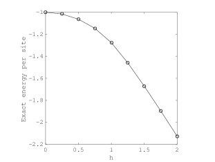
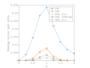
Figure 4.1: TFI model on periodic $12\times 1$ lattice. Approximate energies are computed via the two-cluster-marginal relaxation. Note that ‘p.c.’ indicates the inclusion of the periodicity constraints introduced in section 2.8.1, and ‘overlap’ indicates that the choice of overlapping $2\times 1$ clusters, i.e., $\{1,2\},\{2,3\},\{3,4\},\ldots,\{11,12\},\{12,1\}$.

In Figure 4.2 we test the same relaxations on the same model problem, except that we omit the global semidefinite constraints. Neglecting the global semidefinite constraints correspond to the use of belief propagation (BP) [32] in the classical setting, and its quantum generalization [22, 33, 2, 11]. Note that the omission of these constraints results in a significant degradation of the lower bound, even though the Hamiltonian is local.

Figure 4.2: Results for the same model and same relaxations as in Figure 4.1, with the modification that the global semidefinite constraints are omitted in all cases. In this experiment the curves for ‘$2\times 1$, p.c.’ and $2\times 1$, overlap’ coincide with that of ‘$2\times 1$.’ Note the change of scale of the vertical axis relative to the analogous plot of Figure 4.1. For clarity, we remark that the value of the ‘$3\times 1$, p.c.’ curve at $h=1$ is 0.0035, compared to the corresponding value (with global constraints active) of 0.0016 depicted in Figure 4.1.

Next we consider the TFI model on a periodic $4\times 3$ square lattice, comparing results of the two-cluster-marginal SDP for various cluster sizes. The results are shown in Figure 4.3. Here we are more limited by the preliminary implementation in what can be tested, though the observations are compatible with those preceding remarks which are applicable. In Figure 4.4, we once again test the effect of removing the global semidefinite constraints, and similar conclusions apply.

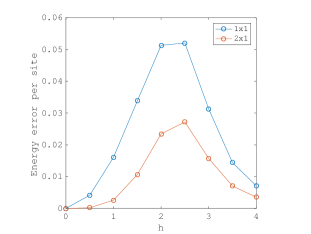
Figure 4.3: TFI model on periodic $4\times 3$ lattice. Approximate energies are computed via the two-cluster-marginal relaxation.

Figure 4.4: Results for the same model and same relaxations as in Figure 4.3, with the modification that the global semidefinite constraints are omitted in all cases. Note the change of scale of the vertical axis relative to the analogous plot of Figure 4.3.

4.2 Anti-ferromagnetic Heisenberg model

First we consider the anti-ferromagnetic Heisenberg model (2.2) on a periodic $12\times 1$ lattice, comparing results of the two-cluster-marginal SDP for various cluster sizes. We also test the periodicity constraints of section 2.8.1 and the case of overlapping clusters, as well as the effect of omitting the global semidefinite constraints. The results are shown in Table 1.

	$1\times 1$	$2\times 1$	$2\times 1$, p.c.	$2\times 1$, overlap	$3\times 1$, p.c.
With global constraints	0.6017	0.0634	0.0462	0.0159	0.0048
Without global constraints	1.2042	0.2042	0.2042	0.2042	0.0310

Table 1: Energy error by cluster specification for the AFH model on periodic $12\times 1$ lattice. For reference, the exact ground state energy is $-1.7958$. Approximate energies for the first line are computed via the two-cluster-marginal relaxation. Note that ‘p.c.’ indicates the inclusion of the periodicity constraints introduced in section 2.8.1, and ‘overlap’ indicates that the choice of overlapping $2\times 1$ clusters, i.e., $\{1,2\},\{2,3\},\{3,4\},\ldots,\{11,12\}$. For the results of the second line, the global semidefinite constraints were omitted.

In Table 2 we show results for the AFH model on a periodic $4\times 3$ lattice for various cluster sizes. For these experiments, the observations are qualitatively similar to those reported for the TFI model, though the relative energy errors are larger. In particular, the errors for $1\times 1$ clusters are quite large, though the error falls dramatically as the cluster size is increased. Moreover, the global constraints achieve significant error reduction even though the Hamiltonian is local.

	$1\times 1$ clusters	$2\times 1$ clusters	$1\times 3$ clusters
With global constraints	1.0439	0.3937	0.0410
Without global constraints	3.5439	2.1897	0.8773

Table 2: Energy error by cluster specification for the AFH model on periodic $4\times 3$ lattice. For reference, the exact ground state energy is $-2.4561$. Approximate energies for the first line are computed via the two-cluster-marginal relaxation. Approximate energies for the second line are obtained by omitting the global semidefinite constraints.

4.3 Hubbard model

Finally we consider the Hubbard model (3.1) on a non-periodic $8\times 1$ lattice with particle numbers $N=6,7,8,9,10$ and interaction strengths $U\in[0,12]$. In Figure 4.5, we plot results for the two-cluster-marginal relaxation with $1\times 1$ clusters $C_{i}:=\{(i,\uparrow),(i,\downarrow)\}$. Observe that for $U=0$, the system is non-interacting and the energy is exact, as guaranteed by the discussion in section 3.4. Furthermore, the error of the energy decreases with respect to $U$ (even without normalizing by $U$). We remark that the error of the energy per site is on par with that of DMET [17] when the same cluster sizes are used. In comparison to DMET, variational embedding is less accurate for intermediate $U$ (i.e., $U\approx 4$) but scales more gracefully in the regime of large $U$ (i.e., $U\gtrsim 8$). However, a thorough comparison of variational embedding with other embedding methods will be a matter for future work following more careful implementation.

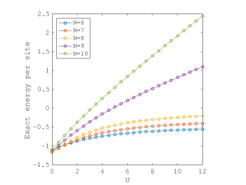
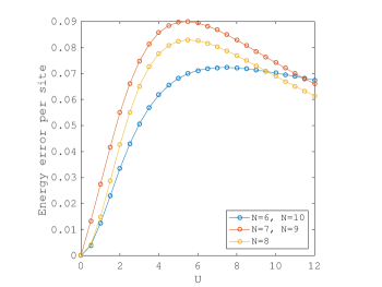
Figure 4.5: Hubbard model on non-periodic $8\times 1$ lattice. Approximate energies are computed via the two-cluster-marginal relaxation with $1\times 1$ clusters $C_{i}:=\{(i,\uparrow),(i,\downarrow)\}$. Note that the energy errors in the cases $N=6$ and $N=7$ coincide with the errors in the cases $N=10$ and $N=9$, respectively due to the particle-hole symmetry.

In Figure 4.6 we test the same relaxation on the same model problems, except that once again we omit the global semidefinite constraints. Once again we observe significant degradation of the lower bound. Note moreover that the omission of these constraints breaks the exactness of the relaxation energy for $U=0$.

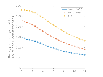
Figure 4.6: Results for the same model and same relaxation as in Figure 4.5, with the modification that the global semidefinite constraints are omitted in all cases. Note the change of scale of the vertical axis relative to the analogous plot of Figure 4.5.

5 Duality and the effective Hamiltonian perspective

In order to reduce the computational cost for solving the SDP in the variational embedding (called the primal problem), we may consider the associated dual problem. For simplicity, we consider duality only for the two-marginal SDP in the quantum spin setting, and it will be convenient to take the ‘abstract perspective’ of section 2.4, with possibly restricted operator sets as in Remark 2. Duality in other settings can be approached by similar means.

5.1 The quantum Kantorovich problem

In preparation for our discussion of the duality of the two-marginal SDP, we first introduce the notion of the quantum Kantorovich problem, which is a direct quantum analog (and in fact generalization) of the Kantorovich problem of optimal transport [41]. See also in [7, 13, 9, 47, 5] for related, though different, presentations.

The analogy to classical optimal transport is defined by replacing probability measures with density operators, a cost function with a cost operator $\hat{C}$, and classical marginalization with quantum marginalization (i.e., the partial trace). Given operators $\mu_{i}\in\mathrm{End}(Q_{i})$ for $i=1,2$ of unit trace, we may define the optimal quantum Kantorovich cost via the SDP

$$\mathbf{QK}[\hat{C}\,;\,\mu_{1},\,\mu_{2}]\ :=\ \underset{\pi\in\mathrm{End}(Q_{1}\otimes Q_{2})}{\mbox{minimize}}\quad \mathrm{Tr}[C\pi]$$

subject to $$\pi\succeq 0$$

$$\mu_{1}=\mathrm{Tr}_{\{2\}}[\pi],\ \mu_{2}=\mathrm{Tr}_{\{1\}}[\pi].$$

Note that if $\mu_{1}\not\succeq 0$ or $\mu_{2}\not\succeq 0$, then since $\pi\succeq 0$ implies that $\mathrm{Tr}_{\{i\}}[\pi]\succeq 0$, the problem is infeasible, i.e., $\mathbf{QK}[C\,;\,\mu_{1},\,\mu_{2}]=+\infty$. Hence without loss of generality one may assume that $\mu_{i}\succeq 0$, i.e., that the $\mu_{i}$ are indeed density operators on $Q_{i}$. Nonetheless, the slightly relaxed perspective will be of some use below. In fact, conversely, the program is feasible whenever $\mu_{1},\mu_{2}\succeq 0$ because in this case $\pi=\mu_{1}\otimes\mu_{2}$ is a feasible point.

There is a notion of quantum Kantorovich duality that analogizes the usual notion, as follows. Let the Hermitian operators $A\in\mathrm{End}(Q_{1})$ and $B\in\mathrm{End}(Q_{2})$ be dual variables for the first and second marginal constraints, respectively. These will be the ‘quantum Kantorovich potentials.’ Dualizing these constraints yields the Lagrangian

$$\mathcal{L}_{\mathrm{QK}}(\pi,A,B)=\mathrm{Tr}[C\pi]+\mathrm{Tr}[A(\mu_{1}-\mathrm{Tr}_{\{2\}}[\pi])]+\mathrm{Tr}[B(\mu_{2}-\mathrm{Tr}_{\{1\}}[\pi])]$$

still constrained by $\pi\succeq 0$. Using the fact that $\mathrm{Tr}[A\,\mathrm{Tr}_{\{2\}}[\pi]]=\mathrm{Tr}[(A\otimes\mathrm{Id})\pi]$ and $\mathrm{Tr}[B\,\mathrm{Tr}_{\{1\}}[\pi]]=\mathrm{Tr}[(\mathrm{Id}\otimes B)\pi]$, we obtain

$$\mathcal{L}_{\mathrm{QK}}(\pi,A,B)=\mathrm{Tr}[A\mu_{1}]+\mathrm{Tr}[B\mu_{2}]+\mathrm{Tr}[\left(C-A\otimes\mathrm{Id}-\mathrm{Id}\otimes B\right)\pi].$$

Now for fixed $A,B$, we have

$$\inf_{\pi\succeq 0}\mathrm{Tr}[\left(C-A\otimes\mathrm{Id}-\mathrm{Id}\otimes B\right)\pi]=\begin{cases}0,&C-A\otimes\mathrm{Id}-\mathrm{Id}\otimes B\succeq 0\\ -\infty,&\mathrm{otherwise}.\end{cases}$$

Hence we have derived the Kantorovich dual problem

$$\underset{A,B\ \mathrm{Hermitian}}{\mbox{maximize}}\quad \mathrm{Tr}[A\mu_{1}]+\mathrm{Tr}[B\mu_{2}]$$ (5.1)

subject to $$A\otimes\mathrm{Id}+\mathrm{Id}\otimes B\preceq C.$$

Strong duality holds by Sion’s minimax theorem [19] (together with the compactness of the feasible set of the primal problem).

Let $\pi$ be the minimizer for the primal problem, and suppose that the dual problem admits a maximizer $(A,B)$. Then let $M=C-A\otimes\mathrm{Id}-\mathrm{Id}\otimes B$, so

$$\mathrm{Tr}[M\pi]=\mathrm{Tr}[C\pi]-\mathrm{Tr}[(A\otimes\mathrm{Id})\pi]-\mathrm{Tr}[(\mathrm{Id}\otimes B)\pi]=\mathrm{Tr}[C\pi]-\mathrm{Tr}[A\mu_{1}]-\mathrm{Tr}[B\mu_{2}]=0,$$

by primal and dual optimality. But $\pi\succeq 0$, so we can write $\pi=\sum_{i=1}^{m}p_{i}\,\phi_{i}\phi_{i}^{*}$ where $p_{i}>0$, and $\mathrm{Tr}[M\pi]=\sum_{i=1}^{m}p_{i}\,\phi_{i}^{*}M\phi_{i}$. But also $M\succeq 0$, so $p_{i}\>\phi_{i}^{*}M\phi_{i}\geq 0$ for all $i=1,\ldots,m$. Then since $\mathrm{Tr}[M\pi]=0$ it follows that $\phi_{i}^{*}M\phi_{i}=0$ for all $i=1,\ldots,m$, and since $M\succeq 0$ this means that $M\phi_{i}=0$ for all $i=1,\ldots,m$.

Therefore $\pi$ is a convex combination of orthogonal projectors onto mutually-orthogonal, degenerate ground state eigenvectors of the Hamiltonian $C-A\otimes\mathrm{Id}-\mathrm{Id}\otimes B$. For the reader familiar with optimal transport, we remark that this observation generalizes the corresponding observation [41] in the classical setting on the support of the Kantorovich coupling, i.e., that $\pi_{ij}\geq 0$ only if $\phi_{i}+\psi_{j}=c_{ij}$, where $\pi=(\pi_{ij})$, $\phi=(\phi_{i})$ and $\psi=(\psi_{i})$ are the Kantorovich potentials, and $c=(c_{ij})$ is the cost matrix.

In fact, one can consider a regularization of the primal problem by a von Neumann entropy penalty (scaled by $\beta$), for which the solution can be shown to be of the form

$$\pi_{\beta}=\frac{1}{Z_{\beta}}\exp\left[-\beta(C-A_{\beta}\otimes\mathrm{Id}-\mathrm{Id}\otimes B_{\beta})\right],$$

where $A_{\beta}$ and $B_{\beta}$ are the unique operators chosen to yield the desired marginals $\mu_{1},\mu_{2}$. This is the quantum analogy of the entropic regularization of classical optimal transport [8]. In the ‘zero-temperature’ limit $\beta\rightarrow\infty$ one expects $\pi_{\beta}\rightarrow\pi$, $A_{\beta}\rightarrow A$, and $B_{\beta}\rightarrow B$.

5.2 Partial duality

Before any derivations, we comment that strong duality (i.e., the fact that there is zero gap between the optimal values of the primal and dual problems for the two-marginal SDP) can be understood as follows. In the original primal problem (2.5), the feasible domain for $\{\rho_{i}\},\,\{\rho_{ij}\}_{i<j}$ in this problem is compact, so strong duality holds simply by Sion’s minimax theorem [19]. The question of whether the dual optimizer is attained is more subtle and will be deferred to future work, though see [15] for the discussion of strong duality in a similar setting.

Now we turn to the derivation of the partial dual problem. We adopt the ‘abstract’ perspective on the global semidefinite constraints introduced in section 2.4, as well as the notation of that section. Referring to (2.5), we first consider a partial Lagrangian obtained by dualizing only the constraint (2.9):

$$\mathcal{L}_{\mathrm{part}}\left(\{\rho_{i}\},\{\rho_{ij}\},X\right)=\sum_{i}\mathrm{Tr}\left[H_{i}\rho_{i}\right]+\sum_{i<j}\mathrm{Tr}\left[H_{ij}\rho_{ij}\right]-\mathrm{Tr}\left(G[\{\rho_{ij}\}]\,X\right),$$

whose domain is defined by $X\in\mathbb{C}^{\left(\sum_{i}m_{i}^{2}\right)\times\left(\sum_{i}m_{i}^{2}\right)}$ Hermitian positive semidefinite and $\{\rho_{i}\},\{\rho_{ij}\}$ satisfying constraints (2.9), (2.9), and (2.9).

Now

$$\mathrm{Tr}\left(G[\{\rho_{ij}\}]\,X\right) = \sum_{ij}\mathrm{Tr}\left(G_{ij}[\rho_{ij}]\,X_{ji}\right)$$

$$= \sum_{i}\sum_{\alpha\beta}\mathrm{Tr}\left[\rho_{i}O_{i,\alpha}^{\dagger}O_{i,\beta}\right](X_{ii})_{\beta\alpha}+\sum_{i\neq j}\sum_{\alpha\beta}\mathrm{Tr}\left[\rho_{ij}\left(O_{i,\alpha}^{\dagger}\otimes O_{j,\beta}\right)\right](X_{ji})_{\beta\alpha}$$

$$= \sum_{i}\sum_{\alpha\beta}\mathrm{Tr}\left[\rho_{i}O_{i,\alpha}^{\dagger}O_{i,\beta}\right](X_{ii})_{\beta\alpha}$$

$$\ \ +\ \sum_{i<j}\sum_{\alpha\beta}\left\{\mathrm{Tr}\left[\rho_{ij}\left(O_{i,\alpha}^{\dagger}\otimes O_{j,\beta}\right)\right](X_{ji})_{\beta\alpha}+\mathrm{Tr}\left[\rho_{ji}\left(O_{j,\beta}^{\dagger}\otimes O_{i,\alpha}\right)\right](X_{ij})_{\alpha\beta}\right\}.$$

Now by the hermiticity of $X$ we have $(X_{ji})_{\beta\alpha}=\overline{(X_{ij})_{\alpha\beta}}$, and we also have the identity

$$\mathrm{Tr}\left[\rho_{ji}\left(O_{j,\beta}^{\dagger}\otimes O_{i,\alpha}\right)\right]=\mathrm{Tr}\left[\rho_{ij}\left(O_{i,\alpha}\otimes O_{j,\beta}^{\dagger}\right)\right].$$

Therefore

$$\mathrm{Tr}\left(G[\{\rho_{ij}\}]\,X\right)=\sum_{i}\mathrm{Tr}\left[Y_{i}(X_{ii})\,\rho_{i}\right]+\sum_{i<j}\mathrm{Tr}\left[Y_{ij}(X_{ij})\,\rho_{ij}\right],$$

where we have defined the functions $Y_{i}:\mathbb{C}^{|\mathcal{I}_{i}|\times|\mathcal{I}_{i}|}\rightarrow\mathrm{End}(Q_{i})$ and $Y_{ij}:\mathbb{C}^{|\mathcal{I}_{i}|\times|\mathcal{I}_{j}|}\rightarrow\mathrm{End}(Q_{i}\otimes Q_{j})$ by

$$Y_{i}(M)=\sum_{\alpha\beta}\overline{M}_{\alpha\beta}\,O_{i,\alpha}^{\dagger}O_{i,\beta},\quad Y_{ij}(M)=\left[\sum_{\alpha\beta}\overline{M}_{\alpha\beta}\,\left(O_{i,\alpha}^{\dagger}\otimes O_{j,\beta}\right)\right]+\mathrm{h.c.},$$

where ‘h.c.’ denotes the Hermitian conjugate. Note that if $M$ is Hermitian, then $Y_{i}(M)$ is Hermitian as well, hence $Y_{i}(X_{ii})$ and $Y_{ij}(X_{ij})$ are Hermitian operators.

By applying Sion’s minimax theorem [19] and then separating the infimum over $\{\rho_{i}\},\{\rho_{ij}\}$ into an outer infimum over $\{\rho_{i}\}$ (subject to constraint (2.9)) and an inner infimum over $\{\rho_{ij}\}$ (subject to constraints (2.9) and (2.9)), we may rewrite the two-marginal SDP energy as

$$E_{0}^{(2)}=\sup_{X\succeq 0}\ \ \underset{\{\rho_{i}\}\,:\,\mathrm{Tr}[\rho_{i}]=1,\forall i}{\inf}\ \ \mathcal{F}\left(X,\{\rho_{i}\}\right),$$ (5.2)

where

$$\mathcal{F}\left(X,\{\rho_{i}\}\right):=\sum_{i}\mathrm{Tr}\left[(H_{i}-Y_{i}(X_{ii}))\rho_{i}\right]+\sum_{i<j}\mathbf{QK}[H_{ij}-Y_{ij}(X_{ij})\,;\,\rho_{i},\,\rho_{j}].$$ (5.3)

This is the form of a concave-convex maxmin problem. The effective domain of the minimization over $\{\rho_{i}\}$ is in fact specified by the constraints $\mathrm{Tr}[\rho_{i}]=1,\ \rho_{i}\succeq 0$ for all $i$, because if $\rho_{i}\not\succeq 0$ for some $i$, then at least one of the quantum Kantorovich problems in the expression for $\mathcal{F}\left(X,\{\rho_{i}\}\right)$ is infeasible, i.e., of infinite optimal cost. The significance of this form is that for fixed $X,\{\rho_{i}\}$, the two-marginals $\rho_{ij}$ have been entirely decoupled from one another in the evaluation of $\mathcal{F}\left(X,\{\rho_{i}\}\right)$. Moreover, for each pair $i<j$, we see the emergence of the effective Hamiltonians $H_{i}^{\mathrm{eff}}(X_{ii}):=H_{i}-Y_{i}(X_{ii})$ and $H_{ij}^{\mathrm{eff}}(X_{ij}):=H_{ij}-Y_{ij}(X_{ij})$ on $Q_{i}$ and $Q_{i}\otimes Q_{j}$, respectively. Notice that the new contributions to these effective Hamiltonians are linear combinations of operators of the form $O_{i,\alpha}^{\dagger}O_{i,\beta}$ and $O_{i,\alpha}^{\dagger}\otimes O_{i,\beta}$, respectively. Thus we see how our choice of effective operator lists is reflected in the richness of our class of possible effective Hamiltonians.

5.3 Computational perspective

From the computational point of view, the partial dual formulation can be much more efficient to solve than the primal formulation. Although general results guarantee that the complexity of solving the two-marginal SDP (2.5) is only polynomial in $M$, direct solution of the primal problem (by, e.g., interior-point methods) may still scale quite poorly in practice. One might hope that the complexity should be limited only by $O(M^{3})$ per iteration, i.e., the cost of diagonalizing a matrix of size proportional to $M$, since the SDP constraint (2.9) concerns a matrix of size proportional to $M$. However, since the semidefinite matrix $G$ is entangled with further equality constraints, the best guarantees for interior-point methods are far more pessimistic. One can interpret our discussion of duality thus far as revealing a special structure of these equality constraints that allows us in principle to design methods achieving a cost of $O(M^{3})$ per iteration. (We remark that similar considerations could be expected to achieve a cost of $O(M)$ per iteration for the quasi-local two-marginal SDP with fixed $d_{\max}$, as described in Remark 3, though we omit details for simplicity.)

Now we describe how to compute gradients of $\mathcal{F}\left(X,\{\rho_{i}\}\right)$, in order to apply, e.g., gradient ascent-descent methods. For fixed $X,\{\rho_{i}\}$, let $(A_{ij}^{\star},B_{ij}^{\star})$ be the unique dual optimizer (assuming that it exists) for the Kantorovich dual formulation of $\mathbf{QK}[H_{ij}-Y_{ij}(X_{ij})\,;\,\rho_{i},\,\rho_{j}]$. Then it follows that

$$\frac{\partial\mathcal{F}}{\partial\rho_{k}}(X,\{\rho_{i}\})=H_{k}-Y_{k}(X_{kk})+\sum_{j>k}A_{kj}^{\star}+\sum_{i<k}B_{ik}^{\star}$$

(Note that if the dual optimizer is not unique, one only gets a supergradient.) One may take a gradient descent step for $\rho_{k}$ in the direction of the traceless part of $\frac{\partial\mathcal{F}}{\partial\rho_{k}}$, adjusting the step size if necessary to guarantee that $\rho_{k}\succeq 0$. Moreover, letting $\rho_{ij}^{\star}$ be the primal solution of the Kantorovich problem indicated by $\mathbf{QK}[H_{ij}-Y_{ij}(X_{ij})\,;\,\rho_{i},\,\rho_{j}]$, we have

$$\frac{\partial\mathcal{F}}{\partial(\overline{X}_{ii})_{\alpha\beta}}(X,\{\rho_{i}\})=-\mathrm{Tr}[O_{i,\alpha}^{\dagger}O_{i,\beta}\,\rho_{i}],\quad\frac{\partial\mathcal{F}}{\partial(\overline{X}_{ij})_{\alpha\beta}}(X,\{\rho_{i}\})=-\mathrm{Tr}\left[\left(O_{i,\alpha}^{\dagger}\otimes O_{j,\beta}\right)\rho_{ij}^{\star}\right].$$

(If the primal optimizer is not unique, one only gets a subgradient.) After taking a gradient ascent step in $X$, one may project onto the feasible domain $\{X\succeq 0\}$ by diagonalizing $X$ and zeroing all negative eigenvalues.

Efficient methods for solving the primal and dual quantum Kantorovich problems (beyond black-box SDP solvers) will be explored in future work. In particular, preliminary results indicate promise for a quantum analog of the classical Sinkhorn scaling algorithm [8], for which the computational cost per iteration is roughly given by the cost of diagonalizing certain operators on $Q_{i}\otimes Q_{j}$.

5.4 Full duality

For completeness we also derive the full dual problem to the original two-marginal SDP. We first introduce dual variables $\lambda_{i}\in\mathbb{R}$ for the constraints $\mathrm{Tr}[\rho_{i}]=1$ appearing in the minimization within (5.2), and then exchange the resulting internal supremum over $\lambda$ with the infimum over $\{\rho_{i}\}$ to obtain the problem:

$$\sup_{X\succeq 0,\,\lambda}\ \ \underset{\{\rho_{i}\}}{\inf}\ \left\{\sum_{i}\lambda_{i}(1-\mathrm{Tr}[\rho_{i}])+\mathcal{F}\left(X,\{\rho_{i}\}\right)\right\}$$

$$= \sup_{X\succeq 0,\,\lambda}\ \left\{\sum_{i}\lambda_{i}+\underset{\{\rho_{i}\}}{\inf}\ \left\{\sum_{i}\mathrm{Tr}\left[(H_{i}-Y_{i}(X_{ii})-\lambda_{i})\rho_{i}\right]+\sum_{i<j}\mathbf{QK}[H_{ij}-Y_{ij}(X_{ij})\,;\,\rho_{i},\,\rho_{j}]\right\}\right\}.$$

Now by substituting the Kantorovich dual expression (5.1) for $\mathbf{QK}$ and then exchanging maximization and minimization, we obtain the problem:

$$\underset{X\succeq 0,\,\lambda\in\mathbb{R}^{M},\,\{A_{ij}\},\,\{B_{ij}\}}{\mbox{maximize}}\quad \sum_{i}\lambda_{i}+\underset{\{\rho_{i}\}}{\inf}\ \left\{\sum_{i}\mathrm{Tr}\left[(H_{i}-Y_{i}(X_{ii})-\lambda_{i})\rho_{i}\right]+\sum_{i<j}\mathrm{Tr}\left[A_{ij}\rho_{i}\right]+\sum_{i<j}\mathrm{Tr}\left[B_{ij}\rho_{j}\right]\right\}$$

subject to $$A_{ij}\otimes\mathrm{Id}+\mathrm{Id}\otimes B_{ij}\preceq H_{ij}-Y_{ij}(X_{ij}),\quad i<j,$$

$$X\succeq 0.$$

Now the expression within the infimum in the objective function can be rewritten

$$\sum_{i}\mathrm{Tr}\left[\left(H_{i}-Y_{i}(X_{ii})-\lambda_{i}+\sum_{j>i}A_{ij}+\sum_{j<i}B_{ji}\right)\rho_{i}\right],$$

so carrying out the infimum within the objective function, we arrive at the full dual:

$$\underset{X\succeq 0,\,\lambda\in\mathbb{R}^{M},\,\{A_{ij}\},\,\{B_{ij}\}}{\mbox{maximize}}\quad \mathbf{1}^{\top}\lambda$$

subject to $$H_{i}-Y_{i}(X_{ii})-\lambda_{i}+\sum_{j>i}A_{ij}+\sum_{j<i}B_{ji}=0,\quad i=1,\ldots,M,$$

$$A_{ij}\otimes\mathrm{Id}+\mathrm{Id}\otimes B_{ij}\preceq H_{ij}-Y_{ij}(X_{ij}),\quad 1\leq i<j\leq M,$$

$$X\succeq 0,$$

where the optimization variables $A_{ij}\in\mathrm{End}(Q_{i})$ and $B_{ij}\in\mathrm{End}(Q_{j})$ are understood to be Hermitian.

References

- [1] J. S. Anderson, M. Nakata, R. Igarashi, K. Fujisawa, and M. Yamashita, The second-order reduced density matrix method and the two-dimensional hubbard model, Comput. Theor. Chem., 1003 (2013), pp. 22–27.
- [2] T. Barthel and R. Hübener, Solving condensed-matter ground-state problems by semidefinite relaxations, Phys. Rev. Lett., 108 (2012), p. 200404.
- [3] G. Biroli, O. Parcollet, and G. Kotliar, Cluster dynamical mean-field theories: Causality and classical limit, Phys. Rev. B, 69 (2004), p. 205108.
- [4] O. Bratteli and D. W. Robinson, Operator algebras and quantum statistical mechanics 1, Springer, 1987.
- [5] E. Caglioti, F. Golse, and T. Paul, Toward optimal transport for quantum densities, hal-01963667, (2018).
- [6] E. Cances, G. Stoltz, and M. Lewin, The electronic ground-state energy problem: A new reduced density matrix approach, J. Chem. Phys., 125 (2006), p. 064101.
- [7] Y. Chen, W. Gangbo, T. Georgiou, and A. Tannenbaum, On the matrix Monge-Kantorovich problem, Eur. J. Appl. Math, (2019).
- [8] M. Cuturi, Sinkhorn distances: Lightspeed computation of optimal transport, Advances in Neural Information Processing Systems, 26 (2013), pp. 2292–2300.
- [9] N. Datta and C. Rouzé, Concentration of quantum states from quantum functional and transportation cost inequalities, J. Math. Phys., 60 (2019), p. 012202.
- [10] A. E. DePrince and D. A. Mazziotti, Exploiting the spatial locality of electron correlation within the parametric two-electron reduced-density-matrix method, J. Chem. Phys., 132 (2010), p. 034110.
- [11] A. J. Ferris and D. Poulin, Algorithms for the Markov entropy decomposition, Phys. Rev. B, 87 (2013), p. 205126.
- [12] A. Georges, G. Kotliar, W. Krauth, and M. J. Rozenberg, Dynamical mean-field theory of strongly correlated fermion systems and the limit of infinite dimensions, Rev. Mod. Phys., 68 (1996), p. 13.
- [13] F. Golse, C. Mouhot, and T. Paul, On the mean field and classical limits of quantum mechanics, Commun. Math. Phys., 343 (2016), pp. 165–205.
- [14] M. Grant and S. Boyd, CVX: Matlab software for disciplined convex programming, 2013.
- [15] Y. Khoo, L. Lin, M. Lindsey, and L. Ying, Semidefinite relaxation of multi-marginal optimal transport for strictly correlated electrons in second quantization, arXiv:1905.08322.
- [16] A. A. Klyachko, Quantum marginal problem and n-representability, J. Phys.: Conf. Ser., 36 (2006), p. 72.
- [17] G. Knizia and G. Chan, Density matrix embedding: A simple alternative to dynamical mean-field theory, Phys. Rev. Lett., 109 (2012), p. 186404.
- [18] G. Knizia and G. K.-L. Chan, Density matrix embedding: A strong-coupling quantum embedding theory, J. Chem. Theory Comput., 9 (2013), pp. 1428–1432.
- [19] H. Komiya, Elementary proof for Sion’s minimax theorem, Kodai Math. J., 11 (1988), pp. 5–7.
- [20] G. Kotliar, S. Y. Savrasov, K. Haule, V. S. Oudovenko, O. Parcollet, and C. A. Marianetti, Electronic structure calculations with dynamical mean-field theory, Rev. Mod. Phys., 78 (2006), p. 865.
- [21] J. B. Lasserre, Moments, Positive Polynomials and Their Applications, Imperial College Press, 2009.
- [22] M. S. Leifer and D. Poulin, Quantum graphical models and belief propagation, Ann. Phys., 323 (2008), p. 1899.
- [23] Y. Li, Z. Wen, C. Yang, and Y.-x. Yuan, A semismooth newton method for semidefinite programs and its applications in electronic structure calculations, SIAM J. Sci. Comput., 40 (2018), pp. A4131–A4157.
- [24] N. Mardirossian, J. D. McClain, and G. Chan, Lowering of the complexity of quantum chemistry methods by choice of representation, J. Chem. Phys., 148 (2018), p. 044106.
- [25] D. Mazziotti, Realization of quantum chemistry without wave functions through first-order semidefinite programming, Phys. Rev. Lett., 93 (2004), p. 213001.
- [26] , Structure of fermionic density matrices: Complete N-representability conditions, Phys. Rev. Lett., 108 (2012), p. 263002.
- [27] D. A. Mazziotti, Contracted Schrödinger equation: Determining quantum energies and two-particle density matrices without wave functions, Phys. Rev. A, 57 (1998), p. 4219.
- [28] M. Nakata, H. Nakatsuji, M. Ehara, M. Fukuda, K. Nakata, and K. Fujisawa, Variational calculations of fermion second-order reduced density matrices by semidefinite programming algorithm, J. Chem. Phys., 114 (2001), pp. 8282–8292.
- [29] J. W. Negele and H. Orland, Quantum many-particle systems, Westview, 1988.
- [30] R. Orús, A practical introduction to tensor networks: Matrix product states and projected entangled pair states, Ann. Phys., 349 (2014), pp. 117–158.
- [31] I. V. Oseledets and E. E. Tyrtyshnikov, Breaking the curse of dimensionality, or how to use svd in many dimensions, SIAM J. Sci. Comput., 31 (2009), pp. 3744–3759.
- [32] J. Pearl, Reverend Bayes on inference engines: a distributed hierarchical approach, Proceedings of the Second National Conference on Artificial Intelligence, (1982), pp. 133–136.
- [33] D. Poulin and M. B. Hastings, Markov entropy decomposition: A variational dual for quantum belief propagation, Phys. Rev. Lett., 106 (2011), p. 080403.
- [34] S. Raghu, S. Kivelson, and D. Scalapino, Superconductivity in the repulsive hubbard model: An asymptotically exact weak-coupling solution, Phy. Rev. B, 81 (2010), p. 224505.
- [35] C. Schilling, The quantum marginal problem, Math. Results Quantum Mech., (2013), pp. 165–176.
- [36] M. Seidl, P. Gori-Giorgi, and A. Savin, Strictly correlated electrons in density-functional theory: A general formulation with applications to spherical densities, Phys. Rev. A, 75 (2007), p. 042511.
- [37] M. Seidl, J. P. Perdew, and M. Levy, Strictly correlated electrons in density-functional theory, Phys. Rev. A, 59 (1999), p. 51.
- [38] Q. Sun and G. K.-L. Chan, Quantum embedding theories, Acc. Chem. Res., 49 (2016), pp. 2705–2712.
- [39] A. Szabo and N. Ostlund, Modern Quantum Chemistry: Introduction to Advanced Electronic Structure Theory, McGraw-Hill, New York, 1989.
- [40] F. Verstraete and J. I. Cirac, Renormalization algorithms for quantum-many body systems in two and higher dimensions, arXiv preprint cond-mat/0407066, (2004).
- [41] C. Villani, Optimal transport: old and new, Springer, 2009.
- [42] M. J. Wainwright and M. I. Jordan, Graphical models, exponential families, and variational inference, Foundations and Trends in Machine Learning, 1-2 (2008), pp. 1–305.
- [43] S. R. White, Density matrix formulation for quantum renormalization groups, Phys. Rev. Lett., 69 (1992), p. 2863.
- [44] S. R. White and E. M. Stoudenmire, Multisliced gausslet basis sets for electronic structure, Phys. Rev. B, 99 (2019), p. 081110.
- [45] H.-Z. Ye, N. D. Ricke, H. K. Tran, and T. Van Voorhis, Bootstrap embedding for molecules, J. Chem. Theory Comput., 15 (2019), pp. 4497–4506.
- [46] Z. Zhao, B. J. Braams, M. Fukuda, M. L. Overton, and J. K. Percus, The reduced density matrix method for electronic structure calculations and the role of three-index representability conditions, J. Chem. Phys., 120 (2004), pp. 2095–2104.
- [47] L. Zhou, S. Ying, N. Yu, and M. Ying, Strassen’s theorem for quantum couplings, Theor. Comput. Sci., (2019).