;

A Relativistic One Dimensional Band Model

with Position Dependent Mass

M. L. Glasser

Department of Physics, Clarkson University

Potsdam, NY 13699-5820 (USA)

laryg@clarkson.edu

Departamento de Física Teórica, Atómica y Óptica and IMUVA,

,

Universidad de Valladolid, 47011 Valladolid, Spain

Abstract

In ths note a one-dimensional band model is proposed based on a periodic Dirac comb having an identical mass distribution $m(x)$ . in each unit cell. The mass function is represented as a Hermitian, non-local separable operator. Two specific cases–a constant mass model and a sinusoidal mass model–are examined. The lowest electron and positron bands for the constant mass case are similar to those for the standard relativistic Kronig-Penney model, suggesting that non-locality has little influence. The results for the sinusoidal case are consistent with the expectation that at low wavenumber an electron “feels” it has am average constant mass, but at high wave number, the particle ”sees” the periodic mass variation and the band is distorted.

Keywords:Relativistic Dirac comb, Kronig-Penney model, enery band structure, position-dependent mass.

PACS No.: 03.65.Fd, 03.65.Pm, 03.65.GePACS No.: 03.65.Fd, 03.65.Pm, 03.65.Ge

Introduction

The desire for considering spatially dependent electron masses in solid state systems was expressed as long ago as the early 1940’s[1] and was made explicit through the work of Wannier, Slater, Luttinger and Kohn [2] with the development of effective mass theory in the early post-war years. Gora and Williams[3] were, it seems, the first to adapt the kinetic energy operator to this situation, but after noting that their original expression was not Hermitian, they proposed the non-relativistic kinetic energy operator

$${\cal K}=-\frac{1}{4\hbar^{2}}[m(\vec{r})^{-1/2}\nabla+\nabla m(\vec{r})^{-1/2}]$$

which was then derived by others from various physical perspectives[4]. O.Von Roos[4] subsequently pointed out that (1) was not unique, being just a special case of

$${\cal K}=-\frac{\hbar^{2}}{4}[m^{a}\nabla m^{b}\nabla m^{c}+m^{c}\nabla m^{b}\nabla m^{a}],\quad a+b+c=-1,$$

On the basis of Bargmann’s theorem[5] he also argued that (2) was unphysical and proved explicitly that the ambiguity was related to a lack of Galilean invariance, i.e. observers in different inertial frames would measure different results for physical properties of such a system. Thus, Von Roos maintained that the very concept of position dependent mass should be avoided as was possible by returning to more fundamental principles. Nevertheless the position dependent mass (PDM) concept has been popular and (2) (usually with $c=a$) has been the basis of a plethora of calculations over the last 30 years. A representative set of papers where PDM is applied to various simple quantum systems is given in[6-12].

In the relativistic case, though Bargmann’s theorem, that physical wave packets cannot be constructed from components corresponding to different masses, still cannot be avoided, at least it can be argued that non-uniqueness is less of a problem since the mass in the Dirac equation occurs simply as a linear operator, similar to the potential[13-15]. The aim here is to take advantage of this by introducing a class of exactly solvable relativistic Kronig-Penney models (i.e. where the lattice potential is a periodic Dirac comb with amplitude $v_{0}$) relative to a fixed frame where the mass is replaced by the non-local separable linear operator

$$m(x)\psi(x)=m_{0}\sum_{l=-N}^{N}\mu(x-la)\int_{-\infty}^{\infty}dx^{\prime}\mu(x^{\prime}-la)\psi(x^{\prime}),$$

( $a$ is the lattice spacing, $N\rightarrow\infty$ the number of unit cells). As will be seen, to construct a particular model one need only specify the Fourier coefficients of $\mu(x)$, the mass profile in a unit cell. This note examines the case

$$\mu(x)=\frac{1}{2}[(1+b)+(1-b)\cos(2\pi x/a)],\quad(0<b<1)$$

illustrated in Fig.1 for $b=.1$

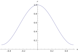
Figure 1: Unit cell mass profile for $b=.1,a=5$.

The Fourier coefficients for (4) are

$$\hat{\mu}_{n}=2\frac{2\pi^{2}(b+1)-a^{2}bk_{n}^{2}}{k_{n}(4\pi^{2}-a^{2}k_{n}^{2})}\sin(k_{n}a/2)$$

$k_{n}=k+K_{n}$ and $K_{n}=2\pi n/a$ is the n-th reciprocal lattice vector.. The constant mass case corresponds to $b=1$.

We present the details of the calculation in the next section, followed by the numerical examination of the specific case (4); the results are discussed in the concluding section.

Calculation

The one-dimensional Dirac equation can be written

$$i\hbar c\phi_{1}^{\prime}=[E-m(x)c^{2}-V(x)]\phi_{2}(x)$$

$$i\hbar c\phi_{2}^{\prime}=[E+m(x)c^{2}-V(x)]\phi_{1}(x)$$

and after inserting the Bloch form of the wave function components,

$$\phi_{j}(x)=\sum_{n}C^{j}_{n}e^{ik_{n}x},$$

where $k$ is the crystal momentum (for simplicity we write $k_{n}=k+K_{n}$) one has

$$\sum_{n}[\hbar ck_{n}C^{1}_{n}+EC^{2}_{n}]e^{ik_{n}x}=\sum_{l,n}C_{n}^{2}e^{ik_{n}la}\{v_{0}\delta(x-la)+u_{0}\mu(x-la)\hat{\mu}_{n}\}$$

$$\sum_{n}[\hbar ck_{n}C^{2}_{n}+EC^{1}_{n}]e^{ik_{n}x}=\sum_{l,n}C_{n}^{1}e^{ik_{n}la}\{v_{0}\delta(x-la)-u_{0}\mu(x-la)\hat{\mu}_{n}\}$$

where we write $u_{0}=m_{0}c^{2}$. For any integrable function $g(x)$ define

$$\hat{g}_{n}=\int_{-\infty}^{\infty}dx^{\prime}e^{ik_{n}x^{\prime}}g(x^{\prime}).$$

Next, we multiply each of (6a,b) by $\exp[-ik_{m}x]$ and integrate over $x$, noting that

$$\int_{-\infty}^{\infty}dxe^{i(k_{n}-k_{m})x}=Na\delta_{n,m}$$

$$\sum_{l}e^{ik_{n}-k_{m})la}=N$$

to find

$$\hbar ck_{m}C^{1}_{m}+EC^{2}_{m}=\frac{1}{a}\sum_{n}[C^{2}_{n}[v_{0}+u_{0}\hat{\mu}_{n}\hat{\mu}_{m}^{*}]$$

$$\hbar ck_{m}C^{2}_{m}+EC^{1}_{m}=\frac{1}{a}\sum_{n}[C^{1}_{n}[v_{0}-u_{0}\hat{\mu}_{n}\hat{\mu}_{m}^{*}]$$

These can be written

$${\cal{M}}{\cal{C}}=\left(\begin{array}[]{c}v_{0}D_{2}+u_{0}d_{2}\hat{\mu}_{m}^{*}\\ v_{0}D_{1}-u_{0}d_{1}\hat{\mu}_{m}^{*}\end{array}\right)$$

with

$$D_{j}=\frac{1}{a}\sum_{n}C^{j}_{n},\quad d_{j}=\frac{1}{a}\sum_{n}C^{j}_{n}\hat{\mu}_{n},$$

$${\cal{M}}=\left(\begin{array}[]{cc}\hbar ck_{m}&E\\ E&\hbar ck_{m}\end{array}\right),\quad{\cal{C}}=\left(\begin{array}[]{c}C^{1}_{m}\\ C^{2}_{m}\end{array}\right).$$

Therefore, by matrix inversion

$$C_{m}^{1}=\frac{1}{\Delta_{m}(k)}\{\hbar ck_{m}[v_{0}D_{2}+u_{0}d_{2}\hat{\mu}_{m}^{*}]-E[v_{0}D_{1}-u_{0}d_{1}\hat{\mu}_{m}^{*}]\}$$

$$C_{m}^{2}=\frac{1}{\Delta_{m}(k)}\{\hbar ck_{m}[v_{0}D_{1}-u_{0}d_{1}\hat{\mu}_{m}^{*}]-E[v_{0}D_{2}+u_{0}d_{2}\hat{\mu}_{m}^{*}]\}$$

where $\Delta_{m}(k)=\hbar^{2}c^{2}k_{m}^{2}-E^{2}.$ So, in terms of the quantities

$$A_{1}^{r}=\sum_{m}\frac{k_{m}^{r}}{\Delta_{m}(k)},\quad A_{2}^{r}=\sum_{m}\frac{k_{m}^{r}|\hat{\mu}_{m}|^{2}}{\Delta_{m}(k)},\quad A_{3}^{r}=\sum_{m}\frac{k_{m}^{r}\hat{\mu}^{*}_{m}}{\Delta_{m}(k)}$$

one has

$$(1+Ev_{0}A_{1}^{0})D_{1}-\hbar cv_{0}A_{1}^{1}D_{2}-Eu_{0}A_{3}^{0}d_{1}-\hbar cu_{0}A_{3}^{1}d_{2}=0$$

$$\hbar cv_{0}A_{1}^{1}D_{1}-(1+Ev_{0}A_{1}^{0})D_{2}-\hbar cu_{0}A_{3}^{1}d_{1}-Eu_{0}A_{3}^{0}d_{2}=0$$

$$Ev_{0}A_{3}^{0}D_{1}+\hbar cv_{0}A_{3}^{1}D_{2}-(1-Eu_{0}A_{3}^{0})d_{1}+\hbar cu_{0}A_{2}^{1}d_{2}=0$$

$$\hbar cv_{0}A_{3}^{1}D_{1}-Ev_{0}A_{3}^{0}D_{2}+\hbar cu_{0}A_{2}^{1}d_{1}-(1+Eu_{0}A_{2}^{0})d_{2}=0$$

Consequently, the band structure is given by the roots $E(k)$ of the $4\times 4$ determinant

$${\cal{D}}(k,\eta)=\left|\begin{array}[]{cccc}1+Ev_{0}A_{1}^{0}&-\hbar cv_{0}A_{1}^{1}&-Eu_{0}A_{3}^{0}&-\hbar cu_{0}A_{3}^{1}\\ -\hbar cv_{0}A_{1}^{1}&1+Ev_{0}A_{1}^{0}&\hbar cu_{0}A_{3}^{1}&Eu_{0}A_{3}^{0}\\ -Ev_{0}A_{3}^{0}&-\hbar cv_{0}A_{3}^{1}&1-Eu_{0}A_{3}^{0}&-\hbar cu_{0}A_{2}^{1}\\ -\hbar cv_{0}A_{3}^{1}&Ev_{0}A_{3}^{0}&-\hbar cu_{0}A_{2}^{1}&1+Eu_{0}A_{2}^{0}\end{array}\right|$$

A word about units is appropriate here. Lengths are given in Bohr radii, $a_{0}$ and we set $\hbar c=1$ so $\eta=E/\hbar c$, $v_{0}$ and $u_{0}$ are all reciprocal lengths.

The six series $A_{i}^{r}$ can be evaluated analytically; for example:

$$A_{1}^{0}=\frac{a}{2\hbar^{2}c^{2}a\eta}\left[\frac{\sin(a\eta)}{\cos(a\eta)-\cos(ka)}\right]$$

$$A_{1}^{1}=\frac{a}{2\hbar^{2}c^{2}}\left[\frac{\sin(ka)}{\cos(a\eta)-\cos(ka)}\right]$$

Numerical Example

As a test case, we set: $a=1,$, $v_{0}=2$,$u_{0}=1000$ and $b=0.1$. Since the ratio $u_{0}/v_{0}=500$ is relatively small, this model may be considered mildly relativistic. The choice $a=1$, which was selected for convenience, means that the lattice is rather dense and may emphasize anomalies. For comparison, we also examine the constant mass version: $b=1$.

The energy levels for the lowest electron band in each case, were found found by plotting the determinant (16), with $k$ specified, as a function of $\eta$ and recording the lowest positive zero. We note that there may be zeros corresponding to vanishing energy denominators $\Delta_{m}(k)=0$, i.e. free, zero-mass bands, which are spurious. Lengths are measured in Bohr radii and we have set $\hbar c=1$, so that energies have units of reciprocal length. For model (3) with $b=1,0.1$, the lowest band $E_{0}(k)$, is shown in Fig. 2, Both bands are continuous and roughly parabolic.

In Fig.(3) we show the next higher band for the two cases. Here again, that for $b=1$ lies above the one for $b=0.1$

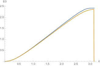
Figure 2: Lowest particle band: $a=1$, $b=.1$(lower curve), $b=1$(upper curve) $v_{0}=2$, $u_{0}=1000$.

Discussion

Since in the constant mass case $b=1$ the lowest band resembles that for the ordinary relativistic Kronig-Penney model [16,17], it appears that the non-local nature of the mass produces no anomalies. However, at the edge of the BZ, $k=\pi/a$, the energy is driven toward zero, as indicated by a vertical line. The relative nature of the two band structures in Fig.2 can be heuristically explained as follows: At low wave vector $k$, for the sinusoidal case the particle has long wave length and ”senses” only tan average mass, so the bands nearly merge, but separate at higher $k$ value where the particle wave length is small enough that the mass variation is detectable. In. which case the energy is depressed. At the zone boundary the particle and mass wavelengths are in resonance and the particle velocity is reduced.

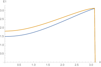
Figure 3: First excited particle band: $a=1$, $b=.1$(initially upper curve), $b=1$( lower curve) $v_{0}=2$, $u_{0}=1000$.

As pointed out in [18] the upper and lower components of the two-component spinor here are particle and anti-particle wave functions, resp. Hence the negative roots of (16) correspond to positron energies. The fundamental bands of the two cases considered here are shown in Fig.4.

In conclusion, a version of the relativistic Kronig-Penney model has been constructed which may be suitable for exploring the effects of variation of effective masses in semiconductor structures. It incorporates the unusual replacement of the mass as a non-local operator, but this does not appear to introduce anomalies in the band structure where the mass has purely sinusoidal variation. In a future report we hope to consider the more usual case where the mass is constant but its value varies from cell to unit cell. Finally, it is worth pointing out that the model is easily extended to two and three dimensions.

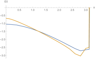
Figure 4: Antiparticle band: $a=1$, $b=.1$(initially upper curve), $b=1$(initially lower curve) $v_{0}=2$, $u_{0}=1000$.

AcknowledgementsThe author thanks Profs. L.M. Nieto and M. Gadella for introducing him to this problem and many helpful suggestions. He also acknowledges the financial support of MINECO (Project MTM2014-57129-C2-1-P) and Junta de Castilla y Leon (VA057U16)).

References

[1] L. Pekar,, J. Phys.(USSR)10, 431 (1946).

[2] G.H. Wannier, Phys.Rev.52,192(1937); J.C. Slater,Phys.Rev.76, 1592(1949); J.M. Luttinger and W. Kohn, Phys.Rev.97,869(1955).

[3] T. Gora and F. Williams, Phys. Rev.177,1179(1969).

[4] O. Von Roos, Position Dependent Effective Masses in Semi-conductor Theory, Phys. Rev.B27,7547-7552(1985); A. Trabelsi, F. Madouri and A. Matar, Classification Scheme for Kinetic Energy Operators with PDM, ArXiv:1302.3763v1(2013).

[5] F.A. Kaempffer,Concepts in Quantum Mechanics,[Academic Press. New York (1965); Appendix 7]

[6] J-M. Levy-Leblonde, Elementary Quantum Models with PDM, Eur. J. Phys. 13,316-318)1992)

[7] R. Koc and H. Tütüncülen, Exact Solution of the PDM Schroedinger Equation by Supersymmetric Quantum Mechanics, ArXiv:quant-phys-0410088v1(2004).

[8] S. Cruz y Cruz, J. Negro and L.M. Nieto,On PDM Harmonic Oscillators ,J. Phys. Conference Series 128, 012053 (2008).

[9] S. Cruz y Cruz and O. Rosas-Ortiz,PDM Oscillators and Coherent States,ArXiv:0902.2029v1(2009).

[10] Ju Guo-Xing, CAI Chang-Ying and REN Zhang-Zhou,Generalized Harmonic Oscillators and the Schroedinger Equation with PDM, Comm. Theor. Phys.(Beijing)51, 797-802(2009).

[11] H. Panahi and Z. Bakhshi,Solvable Potentials with PDM and Constant Mass, Acta Physica Polobica B41,1-21(2010)

[12] S. Cunha and H.R. Christiansen,Analytic Results in the PDM Schroedinger Equation, ArXiv:1306.0933v1(2013).

[13] A.D. Alhaidari, Solution of the Dirac Equation with PDM in the Coulomb Field,Phys. Lett.A322,72-77(2004)

[14] O. Panella, S. Biondini and A. Andra, New Exact Solution of the One-Dimensional Dirac Equation for the Woods-Saxon Potential with the Effective Mass Case, J. Phys, A Math. Theor.43 325902(2010).

[15] M. Eshghi and H. Mehraban,Dirac Poschl-Teller Problem with PDMm Eur.J. Sci. Res.54, 22-28(2011).

[16] F. Dominguez Adame, Amer. J. Phys.55, 1004 (1987)

[17] P. Strange,Relativistic Quantum Mechanics[Cambridge Univ. Press., (1998)] Chap. 9.

[18] M.L. Glasser, A class of one-dimensional relativistic band models, Amer. J. Physics 51, 938 (1983).