Excessive Transverse Coordinates for Orbital Stabilization of (Underactuated) Mechanical Systems

Christian Fredrik Sรฆtre1, Anton Shiriaev1, Stepan Pchelkin1, Ahmed Chemori2 1Department of Engineering Cybernetics, NTNU, Trondheim, Norway. {christian.f.satre,anton.shiriaev,stepan.pchelkin }@ntnu.no2LIRMM, University of Montpellier, CNRS, Montpellier, France. chemori@lirmm.fr
Abstract

Transverse linearization-based approaches have become among the most prominent methods for orbitally stabilizing feedback design in regards to (periodic) motions of underactuated mechanical systems. Yet, in an $n$-dimensional state-space, this requires knowledge of a set of $(n-1)$ independent transverse coordinates, which can be nontrivial to find and whose definitions might vary for different motions (trajectories). In this paper, we consider instead a generic set of excessive transverse coordinates which are defined in terms of a particular parameterization of the motion and a projection operator recovering the โ€œpositionโ€ along the orbit. We present a constructive procedure for obtaining the corresponding transverse linearization, as well as state a sufficient condition for the existence of a feedback controller rendering the desired trajectory (locally) asymptotically orbitally stable. The presented approach is applied to stabilizing oscillations of the underactuated cart-pendulum system about its unstable upright position, in which a novel motion planning approach based on virtual constraints is utilized for trajectory generation.

Index Terms:
Underactuated mechanical systems, orbital stabilization, transverse coordinates, transverse linearization.

I Introduction

We consider the task of generating feedback controllers that orbitally stabilize periodic trajectories of underactuated Euler-Lagrange systems, defined by

$$\mathbf{M}({\mathbf{q}}){\ddot{\mathbf{q}}}+\mathbf{C}({\mathbf{q}},{\dot{\mathbf{q}}}){\dot{\mathbf{q}}}+\mathbf{F}({\mathbf{q}}){\dot{\mathbf{q}}}+\mathbf{G}({\mathbf{q}})=\mathbf{B}{\mathbf{u}}.$$ (1)

Here ${\mathbf{q}}\in\mathbb{R}^{n_{q}}$ and ${\dot{\mathbf{q}}}=\frac{d}{dt}{\mathbf{q}}$ are the generalized coordinates and velocities; ${\mathbf{u}}\in\mathbb{R}^{n_{u}}$ is a vector of $n_{u}(<n_{q})$ control inputs; $\mathbf{M}:\mathbb{R}^{n_{q}}\to\mathbb{R}^{n_{q}\times n_{q}}$ is the symmetric, positive definite inertia matrix; $\mathbf{C}:\mathbb{R}^{n_{q}}\times\mathbb{R}^{n_{q}}\to\mathbb{R}^{n_{q}\times n_{q}}$ is the matrix of Coriolis and centrifugal terms that satisfies $\mathbf{C}({\mathbf{q}},X)Y=\mathbf{C}({\mathbf{q}},Y)X$ for any $X,Y\in\mathbb{R}^{n_{q}}$; $\mathbf{F}:\mathbb{R}^{n_{q}}\to\mathbb{R}^{n_{q}\times n_{q}}$ is a continuously differentiable matrix function of damping and friction terms; $\mathbf{G}:\mathbb{R}^{n_{q}}\to\mathbb{R}^{n_{q}}$ is the gradient of the systemโ€™s potential energy; while $\mathbf{B}\in\mathbb{R}^{n_{q}\times n_{u}}$ is a constant matrix of full rank, i.e. ${\text{rank}~{}{\mathbf{B}}}=\min(n_{q},n_{u})$.

The general problem of stabilizing a predetermined motion (trajectory) of such systems can be highly challenging due to both the nonlinear dynamics and the underactuation. For instance, this prohibits the use of simplifying strategies such feedback linearization, while alternative techniques such as partial feedback linearization [1] will result in some remaining internal dynamics, which can be (made) unstable (non-minimum phase), and consequently must be considered in any control design.

Linearization of the dynamics along a nontrivial solution is also of limited use for the purpose of control design. Indeed, unlike an equilibrium point whose (in-)stability can be determined simply from the stability of the corresponding linearized (first approximation) system, the linear variational system of an autonomous (closed-loop) system evaluated along a periodic solution can never be asymptotically stable, even though the periodic orbit is [2]. This well-known fact can for instance be derived from the Andronov-Vitt theorem, which states that the linear periodic system corresponding to the linearization along a periodic trajectory always will have a non-vanishing, zero-characteristic exponent solution [3].

For such solutions, it can therefore be beneficial to instead consider the stability of the corresponding orbit (the set of all states along the solution). This is the notion of orbital (Poincarรฉ) stability [3, 4], in which asymptotic orbital stability simply means asymptotic convergence to the orbit itself, and not to a specific point in time (moving) along it.

It is well known that a periodic orbit is exponentially stable in the orbital sense if, and only if, the linearization of the dynamics transverse to the orbit is exponentially stable [5]. Indeed, this is true for any orbit if the corresponding linearized system is regular [3, 6]. Thus, if one can find $(2n_{q}-1)$ independent transverse coordinates, which vanish on the nominal orbit, and then exponentially stabilize the origin of the corresponding linearized transverse dynamics (the first approximation system), then one simultaneously asymptotically stabilizes the trajectory in the orbital sense.

Finding a set of $(2n_{q}-1)$ independent transverse coordinates for a particular motion can be nontrivial though. That is, finding a set of coordinates ${\mathbf{x}_{\perp}}\in\mathbb{R}^{2n_{q}-1}$ together with a scalar variable, s๐‘ s, parameterizing the trajectory, such that there exists a (local) diffeomorphism (๐ช,๐ชห™)โ†ฆ(s,๐ฑโŸ‚)maps-to๐ชห™๐ช๐‘ subscript๐ฑperpendicular-to({\mathbf{q}},{\dot{\mathbf{q}}})\mapsto(s,{\mathbf{x}_{\perp}}). However, as we will see, there exists a generic choice of $2n_{q}$ excessive transverse coordinates. Since these excessive coordinates, by definition, are dependent on a minimal set of coordinates, the stability of their origin implies the stability of the origin of the minimal coordinates, and consequently the orbital stability of the desired trajectory.

The same set of excessive coordinates we consider in this paper, together with the linearization of their dynamics, has previously been considered in [7] for stabilizing periodic motions of a fully-actuated robot manipulator. Moreover, they were utilized in [8] for the stabilization of a hybrid walking cycle of a three-link biped robot with two degrees of underactuation, where a particular choice of the parameterizing variable allowed for one coordinate to be trivially omitted in order to obtain a minimal set of transverse coordinates.

In this paper, we build upon and extend the aforementioned works by presenting several original contributions which provide new insights into excessive transverse coordinates and the linearization of their dynamics.

The main contributions of the present paper are:

  • โ€ข

    Providing analytical expressions for the transverse linearization of the excessive transverse coordinates without the need to numerically solve a matrix equation as was required in [7];

  • โ€ข

    Allowing for the projection operator, which recovers the parameterizing variable of the nominal orbit, to be implicitly defined, and which can depend on all of the systemโ€™s states, not only its configuration as in [7];

  • โ€ข

    Illustrating that transverse coordinates need only to be locally transverse to the flow of the nominal orbit rather than restricted to being locally orthogonal as in [5, 9];

  • โ€ข

    Providing an explicit procedure for obtaining an asymptotically orbitally stabilizing feedback controller.

It is also worth noting that the proposed method is not sensitive to singularities in the reduced dynamics (see e.g. [10]). Thus it can be utilized for the stabilization of a richer set of trajectories than the method in [11, 12], such as trajectories whose generating equations have singularities [13] (see also Sec.ย VI) and even certain non-periodic trajectories (assuming the linearization is regular). The method is also easily applicable to systems of any degree of underactuation, as well fully- and redundantly actuated systems, and has the added benefit that any change in actuation will require minor changes in the presented procedure.

A brief outline of the paper follows. We begin by defining a set of excessive transverse coordinates for a given trajectory in Sec.ย II and then derive the linearization of their dynamics in Sec.ย III. We then state the main result of this paper in Sec.ย IV on the form of Theoremย 1, which gives sufficient conditions for attaining an orbitally stabilizing controller. In Sec.ย V we provide conditions that allows for the construction of projection operators. While lastly, in Sec.ย VI, we illustrate the proposed procedure by stabilizing upright oscillations of the underactuated cart-pendulum system.

II Excessive transverse Coordinates

Let ${\mathbf{x}}=[{\mathbf{q}}^{\mathsf{T}},{\dot{\mathbf{q}}}^{\mathsf{T}}]^{\mathsf{T}}\in\mathbb{R}^{2n_{q}}$ denote the state vector of (1), and suppose a non-trivial (non-vanishing), $T$-periodic trajectory

$${\mathbf{x}}_{*}(t,{\mathbf{x}}_{0})={\mathbf{x}}_{*}(t+T,{\mathbf{x}}_{0}),\ {\mathbf{x}}_{*}(0,{\mathbf{x}}_{0})={\mathbf{x}}_{0},\ T>0,$$

is known, as well as the corresponding nominal control input ${\mathbf{u}}_{*}(t,{\mathbf{x}}_{0})$. Further suppose that the corresponding orbit (the set of all states along the trajectory), denoted $\eta_{*}$, admits a reparametrization in terms of a (strictly) monotonically increasing scalar variable sโˆˆ๐’ฎ๐‘ ๐’ฎs\in\mathcal{S}. We will refer to the parameterizing variable, s๐‘ s, as the the motion generator (MG) of the reparameterized trajectory, defined by

๐ฑsโ€‹(s)=[๐ชโˆ—โ€‹(s)๐ชห™โˆ—โ€‹(s)]=[๐šฝโ€‹(s)๐šฝโ€ฒโ€‹(s)โ€‹ฯโ€‹(s)].subscript๐ฑ๐‘ ๐‘ matrixsubscript๐ช๐‘ subscriptห™๐ช๐‘ matrix๐šฝ๐‘ superscript๐šฝโ€ฒ๐‘ ๐œŒ๐‘ \mathbf{x}_{s}(s)=\begin{bmatrix}{\mathbf{q}}_{*}(s)\\ {\dot{\mathbf{q}}}_{*}(s)\end{bmatrix}=\begin{bmatrix}{\mathbf{\Phi}}(s)\\ {\mathbf{\Phi}}^{\prime}(s){\rho}(s)\end{bmatrix}. (2)

Here ๐šฝโ€ฒโ€‹(s)=ddโ€‹sโ€‹๐šฝโ€‹(s)superscript๐šฝโ€ฒ๐‘ ๐‘‘๐‘‘๐‘ ๐šฝ๐‘ {\mathbf{\Phi}}^{\prime}(s)=\frac{d}{ds}{\mathbf{\Phi}}(s) with ${\mathbf{\Phi}}:\mathcal{S}\to\mathbb{R}^{n_{q}}$ at least thrice continuously differentiable, while ${\rho}:\mathcal{S}\to\mathbb{R}$ is a $\mathcal{C}^{2}$-function that recovers the nominal velocity of the MG along the orbit, i.e. sห™โˆ—โ€‹(t)=ฯโ€‹(sโ€‹(t))>0subscriptห™๐‘ ๐‘ก๐œŒ๐‘ ๐‘ก0\dot{s}_{*}(t)={\rho}(s(t))>0, and whose existence is guaranteed by the monotonicity of s๐‘ s and the existence of the orbit $\eta_{*}$, defined by ฮทโˆ—:={๐ฑโˆˆโ„2โ€‹nq:๐ฑ=๐ฑsโ€‹(s),sโˆˆ๐’ฎ}assignsubscript๐œ‚conditional-set๐ฑsuperscriptโ„2subscript๐‘›๐‘žformulae-sequence๐ฑsubscript๐ฑ๐‘ ๐‘ ๐‘ ๐’ฎ\eta_{*}:=\{{\mathbf{x}}\in\mathbb{R}^{2n_{q}}:\ {\mathbf{x}}=\mathbf{x}_{s}(s),\ s\in\mathcal{S}\}.

Note that we will use the subscript-notation โ€œs๐‘ sโ€ throughout this paper to denote that a function is evaluated along the trajectory parameterized by the MG, e.g. hsโ€‹(s):=hโ€‹(๐ฑsโ€‹(s))assignsubscriptโ„Ž๐‘ ๐‘ โ„Žsubscript๐ฑ๐‘ ๐‘ h_{s}(s):=h(\mathbf{x}_{s}(s)) for any $h:\mathbb{R}^{2n_{q}}\to H$ and an arbitrary space $H$. Moreover, we use hsโ€ฒโ€‹(s)=dโ€‹hsdโ€‹sโ€‹(s)superscriptsubscriptโ„Ž๐‘ โ€ฒ๐‘ ๐‘‘subscriptโ„Ž๐‘ ๐‘‘๐‘ ๐‘ h_{s}^{\prime}(s)=\frac{dh_{s}}{ds}(s) for any smooth function hs:๐’ฎโ†’H:subscriptโ„Ž๐‘ โ†’๐’ฎ๐ปh_{s}:\mathcal{S}\to H.

Suppose that within some tubular neighbourhood $\mathcal{X}\subset\mathbb{R}^{2n_{q}}$ of the orbit $\mathbf{\eta}_{*}$, the MG, s๐‘ s, can be found from a projection of the system states upon the orbit by an operator

$$P:\mathbb{R}^{2n_{q}}\to\mathcal{S},\quad{\mathbf{x}}\mapsto P({\mathbf{x}}),\quad\forall{\mathbf{x}}\in\mathcal{X},$$ (3)

which is twice continuously differentiable in $\mathcal{X}$ and satisfies s=Pโ€‹(๐ฑsโ€‹(s))๐‘ ๐‘ƒsubscript๐ฑ๐‘ ๐‘ s=P(\mathbf{x}_{s}(s)) for all sโˆˆ๐’ฎ๐‘ ๐’ฎs\in\mathcal{S}. We will denote by $\mathbf{D}P(\cdot)=\Big{[}\frac{\partial P}{\partial{\mathbf{q}}}(\cdot),\frac{\partial P}{\partial{\dot{\mathbf{q}}}}(\cdot)\Big{]}$ the Jacobian of the mapping $P(\cdot)$ and by $\mathbf{D}^{2}P(\cdot)=\frac{\partial^{2}P}{\partial{\mathbf{x}}^{2}}(\cdot)$ its $2n_{q}\times 2n_{q}$ symmetric Hessian matrix.

The idea behind this projection operator is simply that it allows one to project the current state, at least within some tubular neighbourhood, down upon the nominal orbit to recover the โ€œpositionโ€ along it. This then allows one to define some measure of the distance to this orbit, which, unlike regular reference tracking, will only depend on the current state of the system and not on some time-varying reference, thus giving rise to a completely state-dependent feedback and consequently an autonomous closed-loop system. More specifically, consider

๐ฑโŸ‚:=๐ฑโˆ’๐ฑsโ€‹(s),assignsubscript๐ฑperpendicular-to๐ฑsubscript๐ฑ๐‘ ๐‘ {\mathbf{x}_{\perp}}:={\mathbf{x}}-\mathbf{x}_{s}(s), (4)

which for a particular mapping $P(\cdot)$ are well defined for all ${\mathbf{x}}\in\mathcal{X}$. Differentiating (4) with respect to time leads to

$${\dot{\mathbf{x}}_{\perp}}=\left({{\bf I}}_{2n_{q}}-\mathbf{x}_{s}^{\prime}(s)\mathbf{D}P({\mathbf{x}})\right){\dot{\mathbf{x}}}=:\mathbf{\Omega}({\mathbf{x}}){\dot{\mathbf{x}}},$$ (5)

where ${{\bf I}}_{m}$ is the $m\times m$ identity matrix. It follows that sufficiently close to the orbit, a small variation in the states, $\delta{\mathbf{x}}$, relates to a small variation of the coordinates (4) through

ฮดโ€‹๐ฑโŸ‚=๐›€sโ€‹(s)โ€‹ฮดโ€‹๐ฑ.๐›ฟsubscript๐ฑperpendicular-tosubscript๐›€๐‘ ๐‘ ๐›ฟ๐ฑ\delta{\mathbf{x}_{\perp}}=\mathbf{\Omega}_{s}(s)\delta{\mathbf{x}}. (6)

Here the (Jacobian) matrix function ๐›€sโ€‹(s)subscript๐›€๐‘ ๐‘ \mathbf{\Omega}_{s}(s) is of particular interest. We therefore state some of its key properties next.

Lemma 1

Let $P(\cdot)$ be defined as in (3) and the curve xs:๐’ฎโ†’ฮทโˆ—:subscript๐‘ฅ๐‘ โ†’๐’ฎsubscript๐œ‚x_{s}:\mathcal{S}\to\eta_{*} by (2). Then for all sโˆˆ๐’ฎ๐‘ ๐’ฎs\in\mathcal{S}, the matrix function

๐›€sโ€‹(s):=๐ˆ2โ€‹nqโˆ’๐ฑsโ€ฒโ€‹(s)โ€‹๐ƒโ€‹Psโ€‹(s)assignsubscript๐›€๐‘ ๐‘ subscript๐ˆ2subscript๐‘›๐‘žsuperscriptsubscript๐ฑ๐‘ โ€ฒ๐‘ ๐ƒsubscript๐‘ƒ๐‘ ๐‘ \mathbf{\Omega}_{s}(s):={{\bf I}}_{2n_{q}}-\mathbf{x}_{s}^{\prime}(s)\mathbf{D}P_{s}(s) (7)

is a projection matrix, that is ๐›€s2โ€‹(s)=๐›€sโ€‹(s)superscriptsubscript๐›€๐‘ 2๐‘ subscript๐›€๐‘ ๐‘ \mathbf{\Omega}_{s}^{2}(s)=\mathbf{\Omega}_{s}(s), and its rank is always $(2n_{q}-1)$. Moreover, ๐ƒโ€‹Psโ€‹(s)๐ƒsubscript๐‘ƒ๐‘ ๐‘ \mathbf{D}P_{s}(s) and ๐ฑsโ€ฒโ€‹(s)superscriptsubscript๐ฑ๐‘ โ€ฒ๐‘ \mathbf{x}_{s}^{\prime}(s) are its left- and right annihilators, respectively. โˆŽ

All the properties of ๐›€sโ€‹(โ‹…)subscript๐›€๐‘ โ‹…\mathbf{\Omega}_{s}(\cdot) in the above statement are just straightforward consequences of the relation s=Pโ€‹(๐ฑsโ€‹(s))๐‘ ๐‘ƒsubscript๐ฑ๐‘ ๐‘ s=P(\mathbf{x}_{s}(s)), or equivalently ฯโ€‹(s)=๐ƒโ€‹Psโ€‹(s)โ€‹๐ฑsโ€ฒโ€‹(s)โ€‹ฯโ€‹(s)๐œŒ๐‘ ๐ƒsubscript๐‘ƒ๐‘ ๐‘ superscriptsubscript๐ฑ๐‘ โ€ฒ๐‘ ๐œŒ๐‘ {\rho}(s)=\mathbf{D}P_{s}(s)\mathbf{x}_{s}^{\prime}(s){\rho}(s), and hence

๐ƒโ€‹Psโ€‹(s)โ€‹๐ฑsโ€ฒโ€‹(s)โ‰ก1,โˆ€sโˆˆ๐’ฎ.formulae-sequence๐ƒsubscript๐‘ƒ๐‘ ๐‘ superscriptsubscript๐ฑ๐‘ โ€ฒ๐‘ 1for-all๐‘ ๐’ฎ\mathbf{D}P_{s}(s)\mathbf{x}_{s}^{\prime}(s)\equiv 1,\quad\forall s\in\mathcal{S}. (8)

Here ๐ฑsโ€ฒโ€‹(s)=[๐šฝโ€ฒ๐–ณโ€‹(s),๐šฒ๐–ณโ€‹(s)]๐–ณsuperscriptsubscript๐ฑ๐‘ โ€ฒ๐‘ superscriptsuperscriptsuperscript๐šฝโ€ฒ๐–ณ๐‘ superscript๐šฒ๐–ณ๐‘ ๐–ณ\mathbf{x}_{s}^{\prime}(s)=[{{\mathbf{\Phi}}^{\prime}}^{\mathsf{T}}(s),{\mathbf{\Lambda}}^{\mathsf{T}}(s)]^{\mathsf{T}} with ${\mathbf{\Lambda}}(\cdot)$ defined as

๐šฒโ€‹(s):=๐šฝโ€ฒโ€‹(s)โ€‹ฯโ€ฒโ€‹(s)+๐šฝโ€ฒโ€ฒโ€‹(s)โ€‹ฯโ€‹(s).assign๐šฒ๐‘ superscript๐šฝโ€ฒ๐‘ superscript๐œŒโ€ฒ๐‘ superscript๐šฝโ€ฒโ€ฒ๐‘ ๐œŒ๐‘ {\mathbf{\Lambda}}(s):={\mathbf{\Phi}}^{\prime}(s){\rho}^{\prime}(s)+{\mathbf{\Phi}}^{\prime\prime}(s){\rho}(s). (9)

Note, however, that (8) does not necessarily imply that ๐ƒโ€‹Psโ€‹(s)=๐ฑsโ€ฒ๐–ณโ€‹(s)/โ€–๐ฑsโ€ฒโ€‹(s)โ€–22๐ƒsubscript๐‘ƒ๐‘ ๐‘ superscriptsuperscriptsubscript๐ฑ๐‘ โ€ฒ๐–ณ๐‘ subscriptsuperscriptnormsuperscriptsubscript๐ฑ๐‘ โ€ฒ๐‘ 22\mathbf{D}P_{s}(s)={\mathbf{x}_{s}^{\prime}}^{\mathsf{T}}(s)/\|\mathbf{x}_{s}^{\prime}(s)\|^{2}_{2} in general. Rather, let ฮธโ€‹(s)โˆˆ(โˆ’ฯ€2,ฯ€2)๐œƒ๐‘ ๐œ‹2๐œ‹2\theta(s)\in(-\frac{\pi}{2},\frac{\pi}{2}) denote the angle between ๐ƒโ€‹Psโ€‹(s)๐ƒsubscript๐‘ƒ๐‘ ๐‘ \mathbf{D}P_{s}(s) and ๐ฑsโ€ฒ๐–ณโ€‹(s)superscriptsuperscriptsubscript๐ฑ๐‘ โ€ฒ๐–ณ๐‘ {\mathbf{x}_{s}^{\prime}}^{\mathsf{T}}(s) in their common plane. Then there exists a $\mathcal{C}^{1}$ vector function $\mathbf{n}_{\perp}:\mathcal{S}\to\mathbb{R}^{2n_{q}}$ of unit length within the span of the kernel of ๐ฑsโ€ฒ๐–ณโ€‹(s)superscriptsuperscriptsubscript๐ฑ๐‘ โ€ฒ๐–ณ๐‘ {\mathbf{x}_{s}^{\prime}}^{\mathsf{T}}(s), such that by (8) and the definition of the inner product, we have

๐ƒโ€‹Psโ€‹(s)=๐ฑsโ€ฒโ€‹(s)๐–ณโ€–๐ฑsโ€ฒโ€‹(s)โ€–22+tanโก(ฮธโ€‹(s))โ€‹๐งโŸ‚โ€‹(s)๐–ณโ€–๐ฑsโ€ฒโ€‹(s)โ€–2.๐ƒsubscript๐‘ƒ๐‘ ๐‘ superscriptsubscript๐ฑ๐‘ โ€ฒsuperscript๐‘ ๐–ณsubscriptsuperscriptnormsuperscriptsubscript๐ฑ๐‘ โ€ฒ๐‘ 22๐œƒ๐‘ subscript๐งperpendicular-tosuperscript๐‘ ๐–ณsubscriptnormsuperscriptsubscript๐ฑ๐‘ โ€ฒ๐‘ 2\mathbf{D}P_{s}(s)=\frac{\mathbf{x}_{s}^{\prime}(s)^{\mathsf{T}}}{\|\mathbf{x}_{s}^{\prime}(s)\|^{2}_{2}}+\tan(\theta(s))\frac{\mathbf{n}_{\perp}(s)^{\mathsf{T}}}{\|\mathbf{x}_{s}^{\prime}(s)\|_{2}}. (10)

This simple observation is important, as by Lemmaย 1 and (6) we can infer that ๐›€sโ€‹(s)โ€‹ฮดโ€‹๐ฑโŸ‚=ฮดโ€‹๐ฑโŸ‚subscript๐›€๐‘ ๐‘ ๐›ฟsubscript๐ฑperpendicular-to๐›ฟsubscript๐ฑperpendicular-to\mathbf{\Omega}_{s}(s)\delta{\mathbf{x}_{\perp}}=\delta{\mathbf{x}_{\perp}}, and hence

๐ƒโ€‹Psโ€‹(s)โ€‹ฮดโ€‹๐ฑโŸ‚=๐ƒโ€‹Psโ€‹(s)โ€‹๐›€sโ€‹(s)โ€‹ฮดโ€‹๐ฑโŸ‚โ‰ก0๐ƒsubscript๐‘ƒ๐‘ ๐‘ ๐›ฟsubscript๐ฑperpendicular-to๐ƒsubscript๐‘ƒ๐‘ ๐‘ subscript๐›€๐‘ ๐‘ ๐›ฟsubscript๐ฑperpendicular-to0\mathbf{D}P_{s}(s)\delta{\mathbf{x}_{\perp}}=\mathbf{D}P_{s}(s)\mathbf{\Omega}_{s}(s)\delta{\mathbf{x}_{\perp}}\equiv 0

must hold for all sโˆˆ๐’ฎ๐‘ ๐’ฎs\in\mathcal{S}. This, together with (10), thus allows us to conclude that, sufficiently close to the orbit, the coordinates ${\mathbf{x}_{\perp}}$ are orthogonal to ๐ƒโ€‹Psโ€‹(s)๐ƒsubscript๐‘ƒ๐‘ ๐‘ \mathbf{D}P_{s}(s) and thus transverse to the flow of the orbit; however, they are not necessarily strictly orthogonal to it. Consequently, they constitute a valid set of transverse coordinates, but as the matrix function ๐›€sโ€‹(s)subscript๐›€๐‘ ๐‘ \mathbf{\Omega}_{s}(s) is not invertible (its rank is always $(2n_{q}-1)$), they are an excessive set of transverse coordinates. Nevertheless, as is implied by the following statement (see also [7, Theorem 3]), if the origin of these coordinates is asymptotically stable, then so is also the nominal periodic orbit.

Lemma 2

Let ${\mathbf{y}_{\perp}}:\mathcal{S}\times\mathbb{R}^{2n_{q}}\to\mathbb{R}^{2n_{q}-1}$ be a valid minimal set of transverse coordinates together with a projection operator $P(\cdot)$ as defined in (3). That is, ๐ฑโ†ฆ(s,๐ฒโŸ‚)maps-to๐ฑ๐‘ subscript๐ฒperpendicular-to{\mathbf{x}}\mapsto(s,{\mathbf{y}_{\perp}}) is a local diffeomorphism and ${\mathbf{y}_{\perp}}$ vanishes on $\eta_{*}$. Then the origin of ${\mathbf{y}_{\perp}}$ is asymptotically stable if, and only if, the origin of the excessive coordinates ${\mathbf{x}_{\perp}}$ is asymptotically stable. โˆŽ

The proof of Lemmaย 2 is stated in Appendix A.

The value of these excessive transverse coordinates should therefore be evident: given a known solution to (1), they are a valid set of transverse coordinates for any parameterization of the form (2) and any projection operator (3). They also allow one to easily change between different sets of coordinates by simply changing either (or both) the parameterization or the projection operator.

Thus, with the aim of asymptotically stabilizing the origin of these coordinates, and consequently stabilizing the orbit, we will show next how one can derive the linearization (first approximation) of their dynamics along the target motion.

III Deriving the transverse linearization

Let ๐โ€ โˆˆโ„nuร—nqsuperscript๐โ€ superscriptโ„subscript๐‘›๐‘ขsubscript๐‘›๐‘ž\mathbf{B}^{\dagger}\in\mathbb{R}^{n_{u}\times n_{q}} denote a left-inverse of $\mathbf{B}$, that is ๐โ€ โ€‹๐=๐ˆnusuperscript๐โ€ ๐subscript๐ˆsubscript๐‘›๐‘ข\mathbf{B}^{\dagger}\mathbf{B}={{\bf I}}_{n_{u}}, and define the following matrix function:

๐”โ€‹(๐ช,๐ชห™,s):=๐Œโ€‹(๐ช)โ€‹๐šฒโ€‹(s)โ€‹ฯโ€‹(s)+๐‚โ€‹(๐ช,๐ชห™)โ€‹๐ชห™+๐…โ€‹(๐ช)โ€‹๐ชห™+๐†โ€‹(๐ช).assign๐”๐ชห™๐ช๐‘ ๐Œ๐ช๐šฒ๐‘ ๐œŒ๐‘ ๐‚๐ชห™๐ชห™๐ช๐…๐ชห™๐ช๐†๐ช\mathbf{U}({\mathbf{q}},{\dot{\mathbf{q}}},s):=\mathbf{M}({\mathbf{q}}){\mathbf{\Lambda}}(s){\rho}(s)+\mathbf{C}({\mathbf{q}},{\dot{\mathbf{q}}}){\dot{\mathbf{q}}}+\mathbf{F}({\mathbf{q}}){\dot{\mathbf{q}}}+\mathbf{G}({\mathbf{q}}).

It is not difficult to see that ๐โ€ โ€‹๐”โ€‹(๐ช,๐šฝโ€ฒโ€‹(s)โ€‹ฯโ€‹(s),s)superscript๐โ€ ๐”๐ชsuperscript๐šฝโ€ฒ๐‘ ๐œŒ๐‘ ๐‘ \mathbf{B}^{\dagger}\mathbf{U}({\mathbf{q}},{\mathbf{\Phi}}^{\prime}(s){\rho}(s),s) corresponds to the nominal control input ${\mathbf{u}}_{*}$ when on the nominal orbit. Thus, consider the feedback transformation

๐ฎ=๐โ€ โ€‹๐”^โ€‹(๐ฑ,s)+๐ฏ๐ฎsuperscript๐โ€ ^๐”๐ฑ๐‘ ๐ฏ{\mathbf{u}}=\mathbf{B}^{\dagger}\hat{\mathbf{U}}({\mathbf{x}},s)+{\mathbf{v}} (11)

where $\hat{\mathbf{U}}:\mathbb{R}^{2n_{q}}\times\mathcal{S}\to\mathbb{R}^{n_{q}}$ is a smooth function satisfying ๐”^โ€‹(๐ฑsโ€‹(s),s)โ‰ก๐”โ€‹(๐šฝโ€‹(s),๐šฝโ€ฒโ€‹(s)โ€‹ฯโ€‹(s),s)^๐”subscript๐ฑ๐‘ ๐‘ ๐‘ ๐”๐šฝ๐‘ superscript๐šฝโ€ฒ๐‘ ๐œŒ๐‘ ๐‘ \hat{\mathbf{U}}(\mathbf{x}_{s}(s),s)\equiv\mathbf{U}({\mathbf{\Phi}}(s),{\mathbf{\Phi}}^{\prime}(s){\rho}(s),s) for all sโˆˆ๐’ฎ๐‘ ๐’ฎs\in\mathcal{S}, while ${\mathbf{v}}\in\mathbb{R}^{n_{u}}$ is some stabilizing control input to be defined.111Some natural choices for the function $\hat{\mathbf{U}}$ are ๐”โ€‹(๐šฝโ€‹(s),๐šฝโ€ฒโ€‹(s)โ€‹ฯโ€‹(s),s)๐”๐šฝ๐‘ superscript๐šฝโ€ฒ๐‘ ๐œŒ๐‘ ๐‘ \mathbf{U}({\mathbf{\Phi}}(s),{\mathbf{\Phi}}^{\prime}(s){\rho}(s),s), ๐”โ€‹(๐ช,๐šฝโ€ฒโ€‹(s)โ€‹ฯโ€‹(s),s)๐”๐ชsuperscript๐šฝโ€ฒ๐‘ ๐œŒ๐‘ ๐‘ \mathbf{U}({\mathbf{q}},{\mathbf{\Phi}}^{\prime}(s){\rho}(s),s) or simply ๐”โ€‹(๐ช,๐ชห™,s)๐”๐ชห™๐ช๐‘ \mathbf{U}({\mathbf{q}},{\dot{\mathbf{q}}},s).

Proposition 1 (Excessive transverse linearization)

With the control law (11), the first approximation (linearization) of the dynamics of the transverse coordinates (4) along the trajectory (2) can be written as the constrained (differential-algebraic) linear periodic system

$\displaystyle\frac{d}{dt}\delta{\mathbf{x}_{\perp}}$ =๐€โŸ‚โ€‹(s)โ€‹ฮดโ€‹๐ฑโŸ‚+๐โŸ‚โ€‹(s)โ€‹๐ฏabsentsubscript๐€perpendicular-to๐‘ ๐›ฟsubscript๐ฑperpendicular-tosubscript๐perpendicular-to๐‘ ๐ฏ\displaystyle=\mathbf{A}_{\perp}(s)\delta{\mathbf{x}_{\perp}}+\mathbf{B}_{\perp}(s){\mathbf{v}} (12)
$\displaystyle 0$ =๐ƒโ€‹Psโ€‹(s)โ€‹ฮดโ€‹๐ฑโŸ‚absent๐ƒsubscript๐‘ƒ๐‘ ๐‘ ๐›ฟsubscript๐ฑperpendicular-to\displaystyle=\mathbf{D}P_{s}(s)\delta{\mathbf{x}_{\perp}}

where

๐€โŸ‚โ€‹(s):=๐›€sโ€‹(s)โ€‹๐€โ€‹(s)โˆ’๐ฑsโ€ฒโ€‹(s)โ€‹๐ฑsโ€ฒ๐–ณโ€‹(s)โ€‹๐ƒ2โ€‹Psโ€‹(s)โ€‹ฯโ€‹(s),assignsubscript๐€perpendicular-to๐‘ subscript๐›€๐‘ ๐‘ ๐€๐‘ superscriptsubscript๐ฑ๐‘ โ€ฒ๐‘ superscriptsuperscriptsubscript๐ฑ๐‘ โ€ฒ๐–ณ๐‘ superscript๐ƒ2subscript๐‘ƒ๐‘ ๐‘ ๐œŒ๐‘ \displaystyle\mathbf{A}_{\perp}(s):=\mathbf{\Omega}_{s}(s)\mathbf{A}(s)-\mathbf{x}_{s}^{\prime}(s){\mathbf{x}_{s}^{\prime}}^{\mathsf{T}}(s)\mathbf{D}^{2}P_{s}(s){\rho}(s),
$\displaystyle\mathbf{A}(s)\left.:=\begin{bmatrix}{{\bf 0}}_{n_{q}}&{{\bf I}}_{n_{q}}\\ {\mathbf{M}({\mathbf{q}})}^{-1}\frac{\partial\tilde{\mathbf{U}}}{\partial{\mathbf{q}}}({\mathbf{x}},s)&{\mathbf{M}({\mathbf{q}})}^{-1}\frac{\partial\tilde{\mathbf{U}}}{\partial{\dot{\mathbf{q}}}}({\mathbf{x}},s)\end{bmatrix}\right\lvert_{{\mathbf{x}}=\mathbf{x}_{s}(s)},$
$\displaystyle\mathbf{B}_{\perp}(s):=\left.\mathbf{\Omega}_{s}(s)\begin{bmatrix}{{\bf 0}}_{n_{q}\times n_{u}}\\ \mathbf{M}({\mathbf{q}})^{-1}\mathbf{B}\end{bmatrix}\right\lvert_{{\mathbf{x}}=\mathbf{x}_{s}(s)},$

and ๐”~โ€‹(๐ฑ,s):=๐๐โ€ โ€‹๐”^โ€‹(๐ฑ,s)โˆ’๐”โ€‹(๐ช,๐ชห™,s)assign~๐”๐ฑ๐‘ superscript๐๐โ€ ^๐”๐ฑ๐‘ ๐”๐ชห™๐ช๐‘ \tilde{\mathbf{U}}({\mathbf{x}},s):=\mathbf{B}\mathbf{B}^{\dagger}\hat{\mathbf{U}}({\mathbf{x}},s)-\mathbf{U}({\mathbf{q}},{\dot{\mathbf{q}}},s). โˆŽ

The proof of Propositionย 1 is given in Appendix B.

Remark 1

The matrix function ๐€โŸ‚โ€‹(s)subscript๐€perpendicular-to๐‘ \mathbf{A}_{\perp}(s) in (12) is not unique. That is to say, as ฮดโ€‹๐ฑโŸ‚=๐›€sโ€‹(s)โ€‹ฮดโ€‹๐ฑโŸ‚๐›ฟsubscript๐ฑperpendicular-tosubscript๐›€๐‘ ๐‘ ๐›ฟsubscript๐ฑperpendicular-to\delta{\mathbf{x}_{\perp}}=\mathbf{\Omega}_{s}(s)\delta{\mathbf{x}_{\perp}} and ๐ƒโ€‹Psโ€‹(s)โ€‹ฮดโ€‹๐ฑโŸ‚โ‰ก0๐ƒsubscript๐‘ƒ๐‘ ๐‘ ๐›ฟsubscript๐ฑperpendicular-to0\mathbf{D}P_{s}(s)\delta{\mathbf{x}_{\perp}}\equiv 0, the matrix function ๐€โŸ‚โ€‹(s)โ€‹๐›€sโ€‹(s)+๐—โ€‹(s)โ€‹๐ƒโ€‹Psโ€‹(s)subscript๐€perpendicular-to๐‘ subscript๐›€๐‘ ๐‘ ๐—๐‘ ๐ƒsubscript๐‘ƒ๐‘ ๐‘ \mathbf{A}_{\perp}(s)\mathbf{\Omega}_{s}(s)+\mathbf{X}(s)\mathbf{D}P_{s}(s) would also be a valid choice for any smooth, bounded, vector function $\mathbf{X}:\mathcal{S}\to\mathbb{R}^{2n_{q}}$. โˆŽ

Remark 2

For computing $\mathbf{A}(\cdot)$, it can be useful to note that, by defining ๐ณโŸ‚:=๐ชห™โˆ’๐šฝโ€ฒโ€‹(s)โ€‹ฯโ€‹(s)assignsubscript๐ณperpendicular-toห™๐ชsuperscript๐šฝโ€ฒ๐‘ ๐œŒ๐‘ {\mathbf{z}_{\perp}}:={\dot{\mathbf{q}}}-{\mathbf{\Phi}}^{\prime}(s){\rho}(s), one has

๐”โ€‹(๐ช,๐ชห™,s)=๐”๐ชห™๐ช๐‘ absent\displaystyle\mathbf{U}({\mathbf{q}},{\dot{\mathbf{q}}},s)= ๐”โ€‹(๐ช,๐šฝโ€ฒโ€‹(s)โ€‹ฯโ€‹(s),s)+๐‚โ€‹(๐ช,๐ณโŸ‚)โ€‹๐ณโŸ‚+2โ€‹๐‚โ€‹(๐ช,๐šฝโ€ฒโ€‹(s)โ€‹ฯโ€‹(s))โ€‹๐ณโŸ‚+๐…โ€‹(๐ช)โ€‹๐ณโŸ‚๐”๐ชsuperscript๐šฝโ€ฒ๐‘ ๐œŒ๐‘ ๐‘ ๐‚๐ชsubscript๐ณperpendicular-tosubscript๐ณperpendicular-to2๐‚๐ชsuperscript๐šฝโ€ฒ๐‘ ๐œŒ๐‘ subscript๐ณperpendicular-to๐…๐ชsubscript๐ณperpendicular-to\displaystyle\mathbf{U}({\mathbf{q}},{\mathbf{\Phi}}^{\prime}(s){\rho}(s),s)+\mathbf{C}({\mathbf{q}},{\mathbf{z}_{\perp}}){\mathbf{z}_{\perp}}+2\mathbf{C}({\mathbf{q}},{\mathbf{\Phi}}^{\prime}(s){\rho}(s)){\mathbf{z}_{\perp}}+\mathbf{F}({\mathbf{q}}){\mathbf{z}_{\perp}}

due to $\mathbf{C}({\mathbf{q}},X)Y=\mathbf{C}({\mathbf{q}},Y)X$ for any $X,Y\in\mathbb{R}^{n_{q}}$. โˆŽ

The importance of Propositionย 1 is simply that, by utilizing the structure of the mechanical system (1), it provides explicit expressions for the linearized transverse dynamics of the excessive coordinates (4) which are valid for any trajectory of the form (2), any feedforward-like input $\hat{\mathbf{U}}$, and any projection operator (3). The statement is of course also true for fully actuated systems ($n_{u}\equiv n_{q}$), in which, as then ๐๐โ€ =๐ˆnqsuperscript๐๐โ€ subscript๐ˆsubscript๐‘›๐‘ž\mathbf{B}\mathbf{B}^{\dagger}={{\bf I}}_{n_{q}}, one has the option of using the (partial-) feedback linearizing-like controller ๐”^=๐”โ€‹(๐ช,๐ชห™,s)^๐”๐”๐ชห™๐ช๐‘ \hat{\mathbf{U}}=\mathbf{U}({\mathbf{q}},{\dot{\mathbf{q}}},s), thus resulting in $\tilde{\mathbf{U}}\equiv{{\bf 0}}$.

While it is known [7] that the system (12) can be successfully stabilized in the fully actuated case by a linear feedback of the form ${\mathbf{v}}=\mathbf{K}\delta{\mathbf{x}_{\perp}}$ for some constant $\mathbf{K}\in\mathbb{R}^{n_{q}\times 2n_{q}}$, this will in general not be possible for underactuated systems. Instead, one must find a smooth matrix function $\mathbf{K}:\mathcal{S}\to\mathbb{R}^{n_{u}\times 2n_{q}}$ which varies along the trajectory. We therefore address the issue of how to find such a feedback next.

IV Stabilization of the transverse dynamics

Since we consider periodic orbits, for which it is well known that the (asymptotic) stability of the first approximation implies (asymptotic) stability of the nonlinear system (see e.g. [3]), the following statement naturally holds.

Lemma 3

Suppose that there exists a continuously differentiable matrix function $\mathbf{K}:\mathcal{S}\to\mathbb{R}^{n_{u}\times 2n_{q}}$ such ๐ฏ=๐Šโ€‹(s)โ€‹ฮดโ€‹๐ฑโŸ‚๐ฏ๐Š๐‘ ๐›ฟsubscript๐ฑperpendicular-to{\mathbf{v}}=\mathbf{K}(s)\delta{\mathbf{x}_{\perp}} asymptotically stabilizes the origin of (12). Then the control law (11) with ${\mathbf{v}}=\mathbf{K}(P({\mathbf{x}})){\mathbf{x}_{\perp}}$ renders the nominal orbit $\eta_{*}$ asymptotically stable, and consequently the desired solution ${\mathbf{x}}_{*}(t,{\mathbf{x}}_{0})$ asymptotically orbitally stable. โˆŽ

The question then arises as to how one can find such a matrix function $\mathbf{K}(\cdot)$. If, for instance, the pair $\left(\mathbf{A}_{\perp}(\cdot),\mathbf{B}_{\perp}(\cdot)\right)$ were stabilizable, then it is known (see e.g. [14]) that an exponentially stabilizing controller would be given by

๐ฏ=โˆ’๐šชโˆ’1โ€‹๐โŸ‚๐–ณโ€‹(s)โ€‹๐‘โ€‹(s)โ€‹๐ฑโŸ‚,๐ฏsuperscript๐šช1superscriptsubscript๐perpendicular-to๐–ณ๐‘ ๐‘๐‘ subscript๐ฑperpendicular-to{\mathbf{v}}=-\mathbf{\Gamma}^{-1}\mathbf{B}_{\perp}^{\mathsf{T}}(s)\mathbf{R}(s){\mathbf{x}_{\perp}}, (13)

where the matrix function $\mathbf{R}(\cdot)$ is the symmetric, positive semi-definite solution of the differential Riccati equation

๐‘ห™โ€‹(s)+๐€โŸ‚๐–ณโ€‹(s)โ€‹๐‘โ€‹(s)+๐‘โ€‹(s)โ€‹๐€โŸ‚โ€‹(s)+๐+ฮบโ€‹๐‘โ€‹(s)โˆ’๐‘โ€‹(s)โ€‹๐โŸ‚โ€‹(s)โ€‹๐šชโˆ’1โ€‹๐โŸ‚๐–ณโ€‹(s)โ€‹๐‘โ€‹(s)=0,ห™๐‘๐‘ superscriptsubscript๐€perpendicular-to๐–ณ๐‘ ๐‘๐‘ ๐‘๐‘ subscript๐€perpendicular-to๐‘ ๐๐œ…๐‘๐‘ ๐‘๐‘ subscript๐perpendicular-to๐‘ superscript๐šช1superscriptsubscript๐perpendicular-to๐–ณ๐‘ ๐‘๐‘ 0\displaystyle\dot{\mathbf{R}}(s)+\mathbf{A}_{\perp}^{\mathsf{T}}(s)\mathbf{R}(s)+\mathbf{R}(s)\mathbf{A}_{\perp}(s)+\mathbf{Q}+\kappa\mathbf{R}(s)-\mathbf{R}(s)\mathbf{B}_{\perp}(s)\mathbf{\Gamma}^{-1}\mathbf{B}_{\perp}^{\mathsf{T}}(s)\mathbf{R}(s)=0,

for some $\mathbf{\Gamma}=\mathbf{\Gamma}^{\mathsf{T}}\succ 0$, $\mathbf{Q}=\mathbf{Q}^{\mathsf{T}}\succ 0$ and $\kappa\geq 0$.

Unfortunately, however, it can be shown [15, Proposition 9] (see also Sec. 4.2 in [2]) that the pair $\left(\mathbf{A}_{\perp}(\cdot),\mathbf{B}_{\perp}(\cdot)\right)$ can never be stabilizable even though the origin of the system (12) can be asymptotically (exponentially) stabilized. More precisely, the system ๐ฐห™=๐€โŸ‚โ€‹(s)โ€‹๐ฐ+๐โŸ‚โ€‹(s)โ€‹๐ฏห™๐ฐsubscript๐€perpendicular-to๐‘ ๐ฐsubscript๐perpendicular-to๐‘ ๐ฏ\dot{\mathbf{w}}=\mathbf{A}_{\perp}(s)\mathbf{w}+\mathbf{B}_{\perp}(s){\mathbf{v}}, corresponding to (12) without the transversality condition ๐ƒโ€‹Psโ€‹(s)โ€‹๐ฐ=0๐ƒsubscript๐‘ƒ๐‘ ๐‘ ๐ฐ0\mathbf{D}P_{s}(s)\mathbf{w}=0, always has a non-vanishing solution in the direction of ๐ฑsโ€ฒโ€‹(s)superscriptsubscript๐ฑ๐‘ โ€ฒ๐‘ \mathbf{x}_{s}^{\prime}(s), regardless of the control input ${\mathbf{v}}$.

Although this implies that no solution $\mathbf{R}(\cdot)$ to the above (periodic) differential Riccati equation can exist, we can instead try to find a solution of a modified Riccati equation, which, if found, allows for the generation of a stabilizing controller. This leads us to the main result of this paper.

Theorem 1

Suppose there exists a symmetric, positive semi-definite solution $\mathbf{R}_{\perp}(\cdot)$ to the following modified periodic differential Riccati equation:

๐›€s๐–ณโ€‹(s)โ€‹[๐‘โŸ‚โ€ฒโ€‹(s)โ€‹ฯโ€‹(s)+๐€โŸ‚๐–ณโ€‹(s)โ€‹๐‘โŸ‚โ€‹(s)+๐‘โŸ‚โ€‹(s)โ€‹๐€โŸ‚โ€‹(s)+๐+ฮบโ€‹๐‘โŸ‚โ€‹(s)โˆ’๐‘โŸ‚โ€‹(s)โ€‹๐โŸ‚โ€‹(s)โ€‹๐šชโˆ’1โ€‹๐โŸ‚๐–ณโ€‹(s)โ€‹๐‘โŸ‚โ€‹(s)]โ€‹๐›€sโ€‹(s)=0superscriptsubscript๐›€๐‘ ๐–ณ๐‘ delimited-[]superscriptsubscript๐‘perpendicular-toโ€ฒ๐‘ ๐œŒ๐‘ superscriptsubscript๐€perpendicular-to๐–ณ๐‘ subscript๐‘perpendicular-to๐‘ subscript๐‘perpendicular-to๐‘ subscript๐€perpendicular-to๐‘ ๐๐œ…subscript๐‘perpendicular-to๐‘ subscript๐‘perpendicular-to๐‘ subscript๐perpendicular-to๐‘ superscript๐šช1superscriptsubscript๐perpendicular-to๐–ณ๐‘ subscript๐‘perpendicular-to๐‘ subscript๐›€๐‘ ๐‘ 0\displaystyle\mathbf{\Omega}_{s}^{\mathsf{T}}(s)\Big{[}{\mathbf{R}}_{\perp}^{\prime}(s){\rho}(s)+\mathbf{A}_{\perp}^{\mathsf{T}}(s)\mathbf{R}_{\perp}(s)+\mathbf{R}_{\perp}(s)\mathbf{A}_{\perp}(s)+\mathbf{Q}+\kappa\mathbf{R}_{\perp}(s)-\mathbf{R}_{\perp}(s)\mathbf{B}_{\perp}(s)\mathbf{\Gamma}^{-1}\mathbf{B}_{\perp}^{\mathsf{T}}(s)\mathbf{R}_{\perp}(s)\Big{]}\mathbf{\Omega}_{s}(s)=0 (14)

with ๐‘โŸ‚โ€ฒโ€‹(s)=ddโ€‹sโ€‹๐‘โŸ‚โ€‹(s)superscriptsubscript๐‘perpendicular-toโ€ฒ๐‘ ๐‘‘๐‘‘๐‘ subscript๐‘perpendicular-to๐‘ {\mathbf{R}}_{\perp}^{\prime}(s)=\frac{d}{ds}{\mathbf{R}}_{\perp}(s) and for some $\mathbf{\Gamma}=\mathbf{\Gamma}^{\mathsf{T}}\succ 0$, $\mathbf{Q}=\mathbf{Q}^{\mathsf{T}}\succ 0$ and $\kappa\geq 0$. Then taking

๐ฏ=โˆ’๐šชโˆ’1โ€‹๐โŸ‚๐–ณโ€‹(s)โ€‹๐‘โŸ‚โ€‹(s)โ€‹๐ฑโŸ‚withs=Pโ€‹(๐ฑ)formulae-sequence๐ฏsuperscript๐šช1superscriptsubscript๐perpendicular-to๐–ณ๐‘ subscript๐‘perpendicular-to๐‘ subscript๐ฑperpendicular-towith๐‘ ๐‘ƒ๐ฑ{\mathbf{v}}=-\mathbf{\Gamma}^{-1}\mathbf{B}_{\perp}^{\mathsf{T}}(s)\mathbf{R}_{\perp}(s){\mathbf{x}_{\perp}}\quad\text{with}\quad s=P({\mathbf{x}})

in (11) renders the periodic orbit of the mechanical system (1) corresponding to (2) locally asymptotically stable. โˆŽ

The proof of Theoremย 1 is given in Appendix C.

Naturally, a solution to the projected periodic differential Riccati equation (14) can only exist if the pair (๐€โŸ‚โ€‹(s),๐โŸ‚โ€‹(s))subscript๐€perpendicular-to๐‘ subscript๐perpendicular-to๐‘ (\mathbf{A}_{\perp}(s),\mathbf{B}_{\perp}(s)) is stabilizable on the set of solutions satisfying the condition ๐ƒโ€‹Psโ€‹(s)โ€‹ฮดโ€‹๐ฑโŸ‚โ‰ก0๐ƒsubscript๐‘ƒ๐‘ ๐‘ ๐›ฟsubscript๐ฑperpendicular-to0\mathbf{D}P_{s}(s)\delta{\mathbf{x}_{\perp}}\equiv 0. However, the question of the existence of solutions of this equation is, to our best knowledge, unknown. Although should a solution exist, it is likely not to be unique as the example considered in [15] demonstrates. Nevertheless, as we will see in the example of Sec.ย VI, we have been able to find accurate approximate solutions using numerical methods.

V On Obtaining a Projection operator

So far, we have assumed that a projection operator of the form s=Pโ€‹(๐ฑ)๐‘ ๐‘ƒ๐ฑs=P({\mathbf{x}}), with the mapping $P(\cdot)$ as defined in (3), is known and given as an explicit equation which is well defined within some neighbourhood of the orbit. Yet, this might not necessarily always be the case. That is to say, if one has found a feasible trajectory of the system (1) parameterized on the form (2), the corresponding motion generator might only be known as a function of time, i.e. s=sโ€‹(t)๐‘ ๐‘ ๐‘กs=s(t); indeed, s=t๐‘ ๐‘กs=t is of course the most commonly used parameterization of trajectories. Therefore, we will briefly show next how one can generate projection operators given only knowledge of the nominal trajectory and the time evolution of its parameterizing variable.

In this regard, the following statement follows directly from the implicit function theorem.

Proposition 2

Assume that on a given subarc of the trajectory (2), denoted $\mathcal{S}_{k}\subseteq\mathcal{S}$, there exists a smooth function $h_{k}:\mathbb{R}^{2n_{q}}\times\mathcal{S}_{k}\to\mathbb{R}$ satisfying

hkโ€‹(๐ฑsโ€‹(s),s)โ‰ก0andโˆ‚hkโˆ‚sโ€‹(๐ฑsโ€‹(s),s)โ‰ 0,โˆ€sโˆˆ๐’ฎk.formulae-sequencesubscriptโ„Ž๐‘˜subscript๐ฑ๐‘ ๐‘ ๐‘ 0andformulae-sequencesubscriptโ„Ž๐‘˜๐‘ subscript๐ฑ๐‘ ๐‘ ๐‘ 0for-all๐‘ subscript๐’ฎ๐‘˜h_{k}({\mathbf{x}}_{s}(s),s)\equiv 0\ \ \text{and}\ \ \frac{\partial h_{k}}{\partial s}({\mathbf{x}}_{s}(s),s)\neq 0,\ \ \forall s\in\mathcal{S}_{k}. (15)

Then, in some nonzero, tubular neighbourhood $\mathcal{X}_{k}\subset\mathbb{R}^{2n_{q}}$ of the orbit $\eta_{*}$, there exists a function $P_{k}:\mathcal{X}_{k}\to\mathcal{S}_{k}$ such that for all ${\mathbf{x}}\in\mathcal{X}_{k}$, we have $h_{k}({\mathbf{x}},P_{k}({\mathbf{x}}))=0$ as well as

๐ƒโ€‹Pkโ€‹(๐ฑ)=โˆ’(โˆ‚hkโˆ‚sโ€‹(๐ฑ,Pkโ€‹(๐ฑ)))โˆ’1โ€‹โˆ‚hkโˆ‚๐ฑโ€‹(๐ฑ,Pkโ€‹(๐ฑ)).โˆŽ๐ƒsubscript๐‘ƒ๐‘˜๐ฑsuperscriptsubscriptโ„Ž๐‘˜๐‘ ๐ฑsubscript๐‘ƒ๐‘˜๐ฑ1subscriptโ„Ž๐‘˜๐ฑ๐ฑsubscript๐‘ƒ๐‘˜๐ฑ\mathbf{D}P_{k}({\mathbf{x}})=-{\left(\frac{\partial h_{k}}{\partial s}({\mathbf{x}},P_{k}({\mathbf{x}}))\right)}^{-1}\frac{\partial h_{k}}{\partial{\mathbf{x}}}({\mathbf{x}},P_{k}({\mathbf{x}})).\quad\IEEEQEDclosed

It follows that if a function $h_{k}(\cdot)$ satisfying the conditions of Propositionย 2 for ${\mathbf{x}}(t)\in\mathcal{X}_{k}$ is found, then one can take

s=Pkโ€‹(๐ฑโ€‹(t))๐‘ subscript๐‘ƒ๐‘˜๐ฑ๐‘กs=P_{k}({\mathbf{x}}(t))

as the projection of the states at time $t$ onto the $\mathcal{S}_{k}$ subarc of the orbit (2). Such a function $h(\cdot)$ can often be found satisfying (15) on the whole trajectory. For example, the solution to the following implicit equation

$$s=\operatorname*{arg\,min}_{s\in\mathcal{S}}\left({\mathbf{x}}(t)-{\mathbf{x}}_{s}(s)\right)^{\mathsf{T}}\mathbf{V}(s)\left({\mathbf{x}}(t)-{\mathbf{x}}_{s}(s)\right)$$

with $\mathbf{V}:\mathcal{S}\to\mathbb{R}^{2n_{q}\times 2n_{q}}$ a continuous, symmetric, positive semi-definite matrix functions satisfying ๐ฑsโ€ฒ๐–ณโ€‹(s)โ€‹๐•โ€‹(s)โ€‹๐ฑsโ€ฒโ€‹(s)>0superscriptsuperscriptsubscript๐ฑ๐‘ โ€ฒ๐–ณ๐‘ ๐•๐‘ superscriptsubscript๐ฑ๐‘ โ€ฒ๐‘ 0{\mathbf{x}_{s}^{\prime}}^{\mathsf{T}}(s)\mathbf{V}(s)\mathbf{x}_{s}^{\prime}(s)>0 for all sโˆˆ๐’ฎ๐‘ ๐’ฎs\in\mathcal{S}, is a generic choice for any trajectory of the form (2). Indeed, with $\mathbf{V}={{\bf I}}_{2n_{q}}$, this choice, which has been considered several times before in relation to stability analysis of autonomous dynamical systems (see e.g. [3, 16, 17, 5]), results in the condition ๐ฑsโ€ฒโ€‹(s)๐–ณโ€‹๐ฑโŸ‚โ‰ก0superscriptsubscript๐ฑ๐‘ โ€ฒsuperscript๐‘ ๐–ณsubscript๐ฑperpendicular-to0\mathbf{x}_{s}^{\prime}(s)^{\mathsf{T}}{\mathbf{x}_{\perp}}\equiv 0, and hence

๐ƒโ€‹Pโ€‹(๐ฑ)=๐ฑsโ€ฒ๐–ณโ€‹(s)โ€–๐ฑsโ€ฒโ€‹(s)โ€–22โˆ’๐ฑsโ€ฒโ€ฒโ€‹(s)โ€‹๐ฑโŸ‚.๐ƒ๐‘ƒ๐ฑsuperscriptsuperscriptsubscript๐ฑ๐‘ โ€ฒ๐–ณ๐‘ subscriptsuperscriptnormsuperscriptsubscript๐ฑ๐‘ โ€ฒ๐‘ 22superscriptsubscript๐ฑ๐‘ โ€ฒโ€ฒ๐‘ subscript๐ฑperpendicular-to\mathbf{D}P({\mathbf{x}})=\frac{{\mathbf{x}_{s}^{\prime}}^{\mathsf{T}}(s)}{\|\mathbf{x}_{s}^{\prime}(s)\|^{2}_{2}-\mathbf{x}_{s}^{\prime\prime}(s){\mathbf{x}_{\perp}}}.

Consequently, the projection (3) can be found numerically by, for instance, a few iterations of Newtonโ€™s method.

VI Example: Upright Oscillations of the Cart-Pendulum System

We will now illustrate the procedure outlined in Sec.ย III-IV by stabilizing oscillations around the unstable upright equilibrium of the cart-pendulum system. To keep the derivation short, we consider unit masses, and consider the pendulum bob to be a point mass, while its rod is considered to be massless and of unit length. With the generalized coordinates ${\mathbf{q}}=[x,\theta]^{\mathsf{T}}$ as defined according to Fig.ย 1, the equations of motion of the system are

$\displaystyle 2\ddot{x}+\cos(\theta)\ddot{\theta}-\sin(\theta)\dot{\theta}^{2}$ $\displaystyle=u,$ (16a)
$\displaystyle\ddot{\theta}+\cos(\theta)\ddot{x}-g\sin(\theta)$ $\displaystyle=0,$ (16b)

where g=9.81ย mย sโˆ’2๐‘”times9.81timesmetersecond2g=$9.81\text{\,}\mathrm{m}\text{\,}{\mathrm{s}}^{-2}$ is the gravitational acceleration.

$x$ $\theta$ $g$ $u$
Figure 1: Schematic of the cart-pendulum system, which consists of an unactuated pendulum attached to an actuated cart driven along the horizontal by an external force $u$.

This task has previously been considered in [11] utilizing the virtual constraints approach, where a feasible trajectory of the nonlinear system (16) was generated in the following way. Under the assumption that along a nominal trajectory of the system a set of relations of the form (xโˆ—,ฮธโˆ—)๐–ณ=๐šฝโ€‹(s)=[ฯ•1โ€‹(s),ฯ•2โ€‹(s)]๐–ณsuperscriptsubscript๐‘ฅsubscript๐œƒ๐–ณ๐šฝ๐‘ superscriptsubscriptitalic-ฯ•1๐‘ subscriptitalic-ฯ•2๐‘ ๐–ณ(x_{*},\theta_{*})^{\mathsf{T}}={\mathbf{\Phi}}(s)=[\phi_{1}(s),\phi_{2}(s)]^{\mathsf{T}} are kept invariant, one can write (16b) as

(ฯ•2โ€ฒ+ฯ•1โ€ฒโ€‹cosโก(ฯ•2))โŸฮฑโ€‹(s)โ€‹sยจ+(ฯ•2โ€ฒโ€ฒ+ฯ•1โ€ฒโ€ฒโ€‹cosโก(ฯ•2))โŸฮฒโ€‹(s)โ€‹sห™2โ€‹โˆ’gโ€‹sinโก(ฯ•2)โŸฮณโ€‹(s)=0.subscriptโŸsuperscriptsubscriptitalic-ฯ•2โ€ฒsuperscriptsubscriptitalic-ฯ•1โ€ฒsubscriptitalic-ฯ•2๐›ผ๐‘ ยจ๐‘ subscriptโŸsuperscriptsubscriptitalic-ฯ•2โ€ฒโ€ฒsuperscriptsubscriptitalic-ฯ•1โ€ฒโ€ฒsubscriptitalic-ฯ•2๐›ฝ๐‘ superscriptห™๐‘ 2subscriptโŸ๐‘”subscriptitalic-ฯ•2๐›พ๐‘ 0\underbrace{\left(\phi_{2}^{\prime}+\phi_{1}^{\prime}\cos(\phi_{2})\right)}_{\alpha(s)}\ddot{s}+\underbrace{\left(\phi_{2}^{\prime\prime}+\phi_{1}^{\prime\prime}\cos(\phi_{2})\right)}_{\beta(s)}\dot{s}^{2}\underbrace{-g\sin(\phi_{2})}_{\gamma(s)}=0. (17)

This constrains the time-evolution of the motion generator, s๐‘ s, for the particular choice of ๐šฝโ€‹(s)๐šฝ๐‘ {\mathbf{\Phi}}(s) and its initial velocity sห™0=sห™โ€‹(0)subscriptห™๐‘ 0ห™๐‘ 0\dot{s}_{0}=\dot{s}(0). Moreover, the nominal velocity ฯโ€‹(sโˆ—โ€‹(t))=sห™โˆ—โ€‹(t)๐œŒsubscript๐‘ ๐‘กsubscriptห™๐‘ ๐‘ก{\rho}(s_{*}(t))=\dot{s}_{*}(t) can be found as (17) is integrable [11]; indeed, the equality

$\displaystyle\frac{1}{2}$ expโ€‹{โˆซs0s2โ€‹ฮดโ€‹(ฯƒ)ฮฑโ€‹(ฯƒ)โ€‹๐‘‘ฯƒ}โ€‹ฮฑ2โ€‹(s)โ€‹ฯ2โ€‹(s)โˆ’12โ€‹ฮฑ2โ€‹(s0)โ€‹ฯ2โ€‹(s0)+โˆซs0sexpโ€‹{โˆซs0ฯ„2โ€‹ฮดโ€‹(ฯƒ)ฮฑโ€‹(ฯƒ)โ€‹๐‘‘ฯƒ}โ€‹ฮฑโ€‹(ฯ„)โ€‹ฮณโ€‹(ฯ„)โ€‹๐‘‘ฯ„โ‰ก0expsuperscriptsubscriptsubscript๐‘ 0๐‘ 2๐›ฟ๐œŽ๐›ผ๐œŽdifferential-d๐œŽsuperscript๐›ผ2๐‘ superscript๐œŒ2๐‘ 12superscript๐›ผ2subscript๐‘ 0superscript๐œŒ2subscript๐‘ 0superscriptsubscriptsubscript๐‘ 0๐‘ expsuperscriptsubscriptsubscript๐‘ 0๐œ2๐›ฟ๐œŽ๐›ผ๐œŽdifferential-d๐œŽ๐›ผ๐œ๐›พ๐œdifferential-d๐œ0\displaystyle\text{exp}\left\{\int_{s_{0}}^{s}\frac{2\delta(\sigma)}{\alpha(\sigma)}d\sigma\right\}{\alpha^{2}(s)}{\rho}^{2}(s)-\frac{1}{2}{\alpha^{2}(s_{0})}{\rho}^{2}(s_{0})+\int_{s_{0}}^{s}\text{exp}\left\{\int_{s_{0}}^{\tau}\frac{2\delta(\sigma)}{\alpha(\sigma)}d\sigma\right\}\alpha(\tau)\gamma(\tau)d\tau\equiv 0 (18)

must hold, where ฮดโ€‹(s):=ฮฒโ€‹(s)โˆ’ddโ€‹sโ€‹ฮฑโ€‹(s)assign๐›ฟ๐‘ ๐›ฝ๐‘ ๐‘‘๐‘‘๐‘ ๐›ผ๐‘ \delta(s):=\beta(s)-\frac{d}{ds}\alpha(s). Consequently, the nominal control input uโˆ—=uโˆ—โ€‹(s)subscript๐‘ขsubscript๐‘ข๐‘ u_{*}=u_{*}(s) can be found from (16a).

In [11], the holonomic relations ${\mathbf{\Phi}}(\theta)=[-1.5\sin(\theta),\theta]^{\mathsf{T}}$ were utilized, i.e. the motion generator is simply s=ฮธ๐‘ ๐œƒs=\theta, which results in a center at the equilibrium $\theta=\dot{\theta}=0$.

While s=ฮธ๐‘ ๐œƒs=\theta is clearly a convenient choice in this case, it is not consistent with our parameterization (2) as we require sห™โˆ—>0subscriptห™๐‘ 0\dot{s}_{*}>0. Thus, with sโˆˆ[0,2โ€‹ฯ€)๐‘ 02๐œ‹s\in[0,2\pi) and sห™โˆ—=ฯโ€‹(s)>0subscriptห™๐‘ ๐œŒ๐‘ 0\dot{s}_{*}={\rho}(s)>0, let us instead consider

๐šฝโ€‹(s)=[โˆ’1.5โ€‹sinโก(a2โ€‹cosโก(s)),a2โ€‹cosโก(s)]๐–ณ,๐šฝ๐‘ superscript1.5subscript๐‘Ž2๐‘ subscript๐‘Ž2๐‘ ๐–ณ{\mathbf{\Phi}}(s)=\big{[}-1.5\sin\big{(}a_{2}\cos(s)\big{)},a_{2}\cos(s)\big{]}^{\mathsf{T}}, (19)

which, as we will see, is not holonomic as the projection Pโ€‹(โ‹…)๐‘ƒโ‹…P(\cdot) will depend on (some of) the generalized velocities.
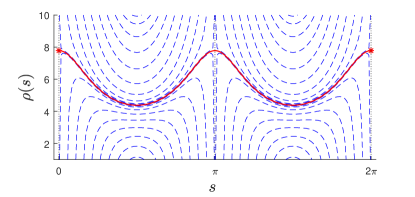
 Hence, we can pick a2subscript๐‘Ž2a_{2} to get the appropriate amplitude of the oscillations of the pendulum, compared to [11] in which the amplitude was determined by the initial conditions (ฮธ0,ฮธห™0)subscript๐œƒ0subscriptห™๐œƒ0(\theta_{0},\dot{\theta}_{0}). Furthermore, while the parameterization in [11] results in a family of periodic solutions around the equilibrium, there exists a unique function ฯโ€‹(s)๐œŒ๐‘ {\rho}(s) for each choice of a2subscript๐‘Ž2a_{2} in the parameterization (19). For example, the unique (positive) solution for the case of a2=0.5subscript๐‘Ž20.5a_{2}=0.5 is the red curve highlighted in Fig.ย 2.

Refer to caption
Figure 2: Solutions of (18) with the parameterization (19). The red curve represents the unique (positive) solution over the interval $[0,2\pi)$ for the case of $a_{2}=0.5$.

It is here worth to note that, even though ฮฑโ€‹(ss)โ‰ก0๐›ผsubscript๐‘ ๐‘ 0\alpha(s_{s})\equiv 0 for ssโˆˆ{0,ฯ€,2โ€‹ฯ€}subscript๐‘ ๐‘ 0๐œ‹2๐œ‹s_{s}\in\{0,\pi,2\pi\}, i.e. sssubscript๐‘ ๐‘ s_{s} are singular points222Note here that the type of (simple) singularities presented here are just a product of the choice of parameterization and not due to the non-uniqueness of (phase-space) solutions as in [13]. of the equation (17), the solution ฯโ€‹(s)๐œŒ๐‘ {\rho}(s) of (18) is well defined over the interval $[0,2\pi)$ if we take ฯโ€‹(s0)๐œŒsubscript๐‘ 0{\rho}(s_{0}) satisfying ฮฒโ€‹(ss)โ€‹ฯ2โ€‹(ss)+ฮณโ€‹(ss)=0๐›ฝsubscript๐‘ ๐‘ superscript๐œŒ2subscript๐‘ ๐‘ ๐›พsubscript๐‘ ๐‘ 0\beta(s_{s}){\rho}^{2}(s_{s})+\gamma(s_{s})=0. Therefore, unlike most existing methods (see, e.g. [11]) which require ฮฑโ€‹(s)โ‰ 0๐›ผ๐‘ 0\alpha(s)\neq 0 for all sโˆˆ๐’ฎ๐‘ ๐’ฎs\in\mathcal{S}, the existence of such singularities is irrelevant for our method.

Now, with the parameterization (19), it is clear that we get ฮธห™โˆ—โ€‹(s)=ฯ•2โ€ฒโ€‹(s)โ€‹ฯโ€‹(s)=โˆ’a2โ€‹sinโก(s)โ€‹ฯโ€‹(s)subscriptห™๐œƒ๐‘ superscriptsubscriptitalic-ฯ•2โ€ฒ๐‘ ๐œŒ๐‘ subscript๐‘Ž2๐‘ ๐œŒ๐‘ \dot{\theta}_{*}(s)=\phi_{2}^{\prime}(s){\rho}(s)=-a_{2}\sin(s){\rho}(s). Hence we can simply find s๐‘ s as the root of the implicit equation

hโ€‹(๐ฑ,s)=sโˆ’arctan2โ€‹(ฮธห™/(โˆ’ฮธโ€‹ฯโ€‹(s)))=0,โ„Ž๐ฑ๐‘ ๐‘ arctan2ห™๐œƒ๐œƒ๐œŒ๐‘ 0h({\mathbf{x}},s)=s-\text{arctan2}\left({\dot{\theta}}/{(-\theta{\rho}(s))}\right)=0,

with $\text{arctan2}(\cdot)$ denoting the four-quadrant arctangent function, thus letting us utilize the method outlined in Sectionย V.

In order to demonstrate the proposed control scheme, we found that taking a2=0.1129subscript๐‘Ž20.1129a_{2}=0.1129 resulted in a periodic orbit very close to the one considered in [11].
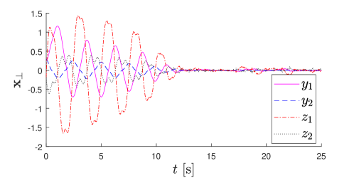
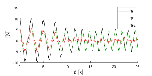
 Figureย 3 shows the results from simulating the system with the initial conditions (x0,ฮธ0,xห™0,ฮธห™0)=(0.1,0.4,โˆ’0.1,โˆ’0.2)x_{0},\theta_{0},\dot{x}_{0},\dot{\theta}_{0})=(0.1,0.4,-0.1,-0.2) and with white noise added to the measurements. The system is seen to converge to the orbit after approximately 13ย stimes13second13\text{\,}\mathrm{s}. Here a feedback LQR-controller of the form (13) was used, which was generated by solving (14) with ๐=๐ˆ4๐subscript๐ˆ4\mathbf{Q}={{\bf I}}_{4}, ฮ“=ฮบ=0.1ฮ“๐œ…0.1\Gamma=\kappa=0.1. This was achieved using the semi-definite programming method of [18] with a trigonometric polynomial of order 40 and utilizing the YALMIP toolbox [19] and the SDPT3 solver [20]. The resulting solution satisfied (14) within a maximum error norm of less than 2ร—10โˆ’42superscript1042\times 10^{-4} for all sโˆˆ[0,2โ€‹ฯ€)๐‘ 02๐œ‹s\in[0,2\pi).

Refer to caption
(a) Phase portraits of the cart (โ€“) and the pendulum (-$\cdot$-).
Refer to caption
(b) Evolution of the transverse coordinates versus time.
Refer to caption
(c) Evolution of the control input signals versus time.
Figure 3: Results from simulating the cart-pendulum system with perturbed initial conditions and noisy measurements.

VII Concluding remarks and future work

In this paper, we have introduced a generic set of excessive transverse coordinates for the purpose of asymptotically orbitally stabilizing periodic trajectories of underactuated Euler-Lagrange systems. We have provided analytical expressions for the corresponding transverse linearization of these coordinates, which are valid regardless of the choice of parameterization of the trajectory, of the choice of the feedforward-like control input, as well as regardless of the choice of projection operator. In addition, we have derived a sufficient condition for the existence of a stabilizing controller for this constrained linear system, allowing for the construction of a feedback controller rendering the desired periodic motion asymptotically (exponentially) stable in the orbital sense. The proposed scheme was applied to the task of stabilizing oscillations of the cart-pendulum system around its unstable upright position and was successfully tested in simulation. This example also illustrated that the proposed methodology can, unlike most other methods, be used to stabilize trajectories for which the reduced dynamics have singular points. Experimental validation of the proposed scheme is currently being pursued.

APPENDIX

Appendix A. proof of Lemmaย 2

It here suffices to show that the asymptotic stability of the variation $\delta{\mathbf{x}_{\perp}}$ is equivalent to that of $\delta{\mathbf{y}_{\perp}}$. Tho this end, we note that by the hypothesis that the mapping (s,๐ฒโŸ‚)โ†ฆ๐ฑmaps-to๐‘ subscript๐ฒperpendicular-to๐ฑ(s,{\mathbf{y}_{\perp}})\mapsto{\mathbf{x}} is a diffeomorphism in a neighbourhood of $\eta_{*}$, it follows that the Jacobian of ${\mathbf{y}_{\perp}}$ evaluated along ๐ฑsโ€‹(s)subscript๐ฑ๐‘ ๐‘ \mathbf{x}_{s}(s), that is

๐ƒ๐ฒโŸ‚โ€‹(s,๐ฑsโ€‹(s))=โˆ‚๐ฒโŸ‚โˆ‚๐ฑโ€‹(s,๐ฑsโ€‹(s))+โˆ‚๐ฒโŸ‚โˆ‚sโ€‹(s,๐ฑsโ€‹(s))โ€‹๐ƒโ€‹Psโ€‹(s),subscript๐ƒ๐ฒperpendicular-to๐‘ subscript๐ฑ๐‘ ๐‘ subscript๐ฒperpendicular-to๐ฑ๐‘ subscript๐ฑ๐‘ ๐‘ subscript๐ฒperpendicular-to๐‘ ๐‘ subscript๐ฑ๐‘ ๐‘ ๐ƒsubscript๐‘ƒ๐‘ ๐‘ \mathbf{D}{\mathbf{y}_{\perp}}(s,\mathbf{x}_{s}(s))=\frac{\partial{\mathbf{y}_{\perp}}}{\partial{\mathbf{x}}}(s,\mathbf{x}_{s}(s))+\frac{\partial{\mathbf{y}_{\perp}}}{\partial s}(s,\mathbf{x}_{s}(s))\mathbf{D}P_{s}(s),

has full (row) rank for all sโˆˆ๐’ฎ๐‘ ๐’ฎs\in\mathcal{S}. But as ๐ฒโŸ‚โ€‹(s,๐ฑsโ€‹(s))โ‰ก0subscript๐ฒperpendicular-to๐‘ subscript๐ฑ๐‘ ๐‘ 0{\mathbf{y}_{\perp}}(s,\mathbf{x}_{s}(s))\equiv 0, we have dโ€‹๐ฒโŸ‚dโ€‹๐ฑโ€‹(s,๐ฑsโ€‹(s))โ€‹๐ฑsโ€ฒโ€‹(s)โ‰ก๐ŸŽ๐‘‘subscript๐ฒperpendicular-to๐‘‘๐ฑ๐‘ subscript๐ฑ๐‘ ๐‘ superscriptsubscript๐ฑ๐‘ โ€ฒ๐‘ 0\frac{d{\mathbf{y}_{\perp}}}{d{\mathbf{x}}}(s,\mathbf{x}_{s}(s))\mathbf{x}_{s}^{\prime}(s)\equiv{{\bf 0}}, such that by (8) and by defining ๐šทsโ€‹(s):=โˆ‚๐ฒโŸ‚โˆ‚๐ฑโ€‹(s,๐ฑsโ€‹(s))assignsubscript๐šท๐‘ ๐‘ subscript๐ฒperpendicular-to๐ฑ๐‘ subscript๐ฑ๐‘ ๐‘ \mathbf{\Pi}_{s}(s):=\frac{\partial{\mathbf{y}_{\perp}}}{\partial{\mathbf{x}}}(s,\mathbf{x}_{s}(s)), we obtain the relation

๐šทsโ€‹(s)โ€‹๐ฑsโ€ฒโ€‹(s)=โˆ’โˆ‚๐ฒโŸ‚โˆ‚sโ€‹(s,๐ฑsโ€‹(s)).subscript๐šท๐‘ ๐‘ superscriptsubscript๐ฑ๐‘ โ€ฒ๐‘ subscript๐ฒperpendicular-to๐‘ ๐‘ subscript๐ฑ๐‘ ๐‘ \mathbf{\Pi}_{s}(s)\mathbf{x}_{s}^{\prime}(s)=-\frac{\partial{\mathbf{y}_{\perp}}}{\partial s}(s,\mathbf{x}_{s}(s)).

This further implies that

ฮดโ€‹๐ฒโŸ‚=๐ƒ๐ฒโŸ‚โ€‹(s,๐ฑsโ€‹(s))โ€‹ฮดโ€‹๐ฑ=๐šทsโ€‹(s)โ€‹๐›€sโ€‹(s)โ€‹ฮดโ€‹๐ฑ,๐›ฟsubscript๐ฒperpendicular-tosubscript๐ƒ๐ฒperpendicular-to๐‘ subscript๐ฑ๐‘ ๐‘ ๐›ฟ๐ฑsubscript๐šท๐‘ ๐‘ subscript๐›€๐‘ ๐‘ ๐›ฟ๐ฑ\delta{\mathbf{y}_{\perp}}=\mathbf{D}{\mathbf{y}_{\perp}}(s,\mathbf{x}_{s}(s))\delta{\mathbf{x}}=\mathbf{\Pi}_{s}(s)\mathbf{\Omega}_{s}(s)\delta{\mathbf{x}},

such that from (6), i.e. ฮดโ€‹๐ฑโŸ‚=๐›€sโ€‹(s)โ€‹ฮดโ€‹๐ฑ๐›ฟsubscript๐ฑperpendicular-tosubscript๐›€๐‘ ๐‘ ๐›ฟ๐ฑ\delta{\mathbf{x}_{\perp}}=\mathbf{\Omega}_{s}(s)\delta{\mathbf{x}}, we obtain

ฮดโ€‹๐ฒโŸ‚=๐šทsโ€‹(s)โ€‹ฮดโ€‹๐ฑโŸ‚.๐›ฟsubscript๐ฒperpendicular-tosubscript๐šท๐‘ ๐‘ ๐›ฟsubscript๐ฑperpendicular-to\delta{\mathbf{y}_{\perp}}=\mathbf{\Pi}_{s}(s)\delta{\mathbf{x}_{\perp}}. (20)

Therefore, from Lemmaย 1 and the fact that ๐šทsโ€‹(s)โ€‹๐›€sโ€‹(s)subscript๐šท๐‘ ๐‘ subscript๐›€๐‘ ๐‘ \mathbf{\Pi}_{s}(s)\mathbf{\Omega}_{s}(s) is of full rank ($2n_{q}-1$), it follows from (20) that $\|\delta{\mathbf{y}_{\perp}}\|\to 0$ as $t\to\infty$ only if $\|\delta{\mathbf{x}_{\perp}}\|\to 0$. Thus it just remains to show that the converse is true as well, namely that $\|\delta{\mathbf{x}_{\perp}}\|\to 0$ as $t\to\infty$ only if $\|\delta{\mathbf{y}_{\perp}}\|\to 0$.

Towards this end, take $\mathbf{p}_{\perp}:\mathcal{S}\to\mathbb{R}^{2n_{q}\times(2n_{q}-1)}$ to be some differentiable basis of the the kernel of ๐ƒโ€‹Psโ€‹(s)๐ƒsubscript๐‘ƒ๐‘ ๐‘ \mathbf{D}P_{s}(s). As then ๐ฉโŸ‚โ€‹(s)=๐›€sโ€‹(s)โ€‹๐ฉโŸ‚โ€‹(s)subscript๐ฉperpendicular-to๐‘ subscript๐›€๐‘ ๐‘ subscript๐ฉperpendicular-to๐‘ \mathbf{p}_{\perp}(s)=\mathbf{\Omega}_{s}(s)\mathbf{p}_{\perp}(s) and rankโ€‹[๐šทsโ€‹(s)โ€‹๐›€sโ€‹(s)]=2โ€‹nqโˆ’1rankdelimited-[]subscript๐šท๐‘ ๐‘ subscript๐›€๐‘ ๐‘ 2subscript๐‘›๐‘ž1{\text{rank}~{}{[}}\mathbf{\Pi}_{s}(s)\mathbf{\Omega}_{s}(s)]=2n_{q}-1, it follows that ๐šทsโ€‹(s)โ€‹๐ฉโŸ‚โ€‹(s)subscript๐šท๐‘ ๐‘ subscript๐ฉperpendicular-to๐‘ \mathbf{\Pi}_{s}(s)\mathbf{p}_{\perp}(s) is invertible for all sโˆˆ๐’ฎ๐‘ ๐’ฎs\in\mathcal{S}. Hence

[๐ƒโ€‹Psโ€‹(s)๐šทsโ€‹(s)โ€‹๐›€sโ€‹(s)]โ€‹[๐ฑsโ€ฒโ€‹(s)๐ฉโŸ‚โ€‹(s)โ€‹(๐šทsโ€‹(s)โ€‹๐ฉโŸ‚โ€‹(s))โˆ’1]=๐ˆ2โ€‹nqโˆ’1,matrix๐ƒsubscript๐‘ƒ๐‘ ๐‘ subscript๐šท๐‘ ๐‘ subscript๐›€๐‘ ๐‘ matrixsuperscriptsubscript๐ฑ๐‘ โ€ฒ๐‘ subscript๐ฉperpendicular-to๐‘ superscriptsubscript๐šท๐‘ ๐‘ subscript๐ฉperpendicular-to๐‘ 1subscript๐ˆ2subscript๐‘›๐‘ž1\begin{bmatrix}\mathbf{D}P_{s}(s)\\ \mathbf{\Pi}_{s}(s)\mathbf{\Omega}_{s}(s)\end{bmatrix}\begin{bmatrix}\mathbf{x}_{s}^{\prime}(s)&\mathbf{p}_{\perp}(s)\left(\mathbf{\Pi}_{s}(s)\mathbf{p}_{\perp}(s)\right)^{-1}\end{bmatrix}={{\bf I}}_{2n_{q}-1},

which implies that

ฮดโ€‹๐ฑ=๐ฉโŸ‚โ€‹(s)โ€‹(๐šทsโ€‹(s)โ€‹๐ฉโŸ‚โ€‹(s))โˆ’1โ€‹ฮดโ€‹๐ฒโŸ‚+๐ฑsโ€ฒโ€‹(s)โ€‹ฮดโ€‹s.๐›ฟ๐ฑsubscript๐ฉperpendicular-to๐‘ superscriptsubscript๐šท๐‘ ๐‘ subscript๐ฉperpendicular-to๐‘ 1๐›ฟsubscript๐ฒperpendicular-tosuperscriptsubscript๐ฑ๐‘ โ€ฒ๐‘ ๐›ฟ๐‘ \delta{\mathbf{x}}=\mathbf{p}_{\perp}(s)\left(\mathbf{\Pi}_{s}(s)\mathbf{p}_{\perp}(s)\right)^{-1}\delta{\mathbf{y}_{\perp}}+\mathbf{x}_{s}^{\prime}(s)\delta s.

Left-multiplying the above equation by ๐›€sโ€‹(s)subscript๐›€๐‘ ๐‘ \mathbf{\Omega}_{s}(s), we obtain

ฮดโ€‹๐ฑโŸ‚=๐ฉโŸ‚โ€‹(s)โ€‹(๐šทsโ€‹(s)โ€‹๐ฉโŸ‚โ€‹(s))โˆ’1โ€‹ฮดโ€‹๐ฒโŸ‚.๐›ฟsubscript๐ฑperpendicular-tosubscript๐ฉperpendicular-to๐‘ superscriptsubscript๐šท๐‘ ๐‘ subscript๐ฉperpendicular-to๐‘ 1๐›ฟsubscript๐ฒperpendicular-to\delta{\mathbf{x}_{\perp}}=\mathbf{p}_{\perp}(s)\left(\mathbf{\Pi}_{s}(s)\mathbf{p}_{\perp}(s)\right)^{-1}\delta{\mathbf{y}_{\perp}}.

It follows that $\|\delta{\mathbf{x}_{\perp}}\|\to 0$ only if $\|\delta{\mathbf{y}_{\perp}}\|\to 0$. โˆŽ

Appendix B. Proof of Propositionย 1

Let ๐ณโŸ‚:=๐ชห™โˆ’๐šฝโ€ฒโ€‹(s)โ€‹ฯโ€‹(s)assignsubscript๐ณperpendicular-toห™๐ชsuperscript๐šฝโ€ฒ๐‘ ๐œŒ๐‘ {\mathbf{z}_{\perp}}:={\dot{\mathbf{q}}}-{\mathbf{\Phi}}^{\prime}(s){\rho}(s) and note that the dynamics of the system (1) then can be rewritten on the form

๐ฑห™=๐ฑsโ€ฒโ€‹(s)โ€‹ฯโ€‹(s)+[๐ณโŸ‚โˆ’๐Œโ€‹(๐ช)โˆ’1โ€‹๐”โ€‹(๐ช,๐ชห™,s)]+[๐ŸŽnqร—nu๐Œโ€‹(๐ช)โˆ’1โ€‹๐]โ€‹๐ฎ.ห™๐ฑsuperscriptsubscript๐ฑ๐‘ โ€ฒ๐‘ ๐œŒ๐‘ matrixsubscript๐ณperpendicular-to๐Œsuperscript๐ช1๐”๐ชห™๐ช๐‘ matrixsubscript0subscript๐‘›๐‘žsubscript๐‘›๐‘ข๐Œsuperscript๐ช1๐๐ฎ{\dot{\mathbf{x}}}=\mathbf{x}_{s}^{\prime}(s){\rho}(s)+\begin{bmatrix}{\mathbf{z}_{\perp}}\\ -\mathbf{M}({\mathbf{q}})^{-1}\mathbf{U}({\mathbf{q}},{\dot{\mathbf{q}}},s)\end{bmatrix}+\begin{bmatrix}{{\bf 0}}_{n_{q}\times n_{u}}\\ \mathbf{M}({\mathbf{q}})^{-1}\mathbf{B}\end{bmatrix}{\mathbf{u}}.

If the controller is taken as in (11), we obtain

๐ฑห™=๐ฑsโ€ฒโ€‹(s)โ€‹ฯโ€‹(s)+๐ŸU~โ€‹(๐ฑ,s)+[๐ŸŽnqร—nu๐Œโ€‹(๐ช)โˆ’1โ€‹๐]โ€‹๐ฏ,ห™๐ฑsuperscriptsubscript๐ฑ๐‘ โ€ฒ๐‘ ๐œŒ๐‘ subscript๐Ÿ~๐‘ˆ๐ฑ๐‘ matrixsubscript0subscript๐‘›๐‘žsubscript๐‘›๐‘ข๐Œsuperscript๐ช1๐๐ฏ{\dot{\mathbf{x}}}=\mathbf{x}_{s}^{\prime}(s){\rho}(s)+\mathbf{f}_{\tilde{U}}({\mathbf{x}},s)+\begin{bmatrix}{{\bf 0}}_{n_{q}\times n_{u}}\\ \mathbf{M}({\mathbf{q}})^{-1}\mathbf{B}\end{bmatrix}{\mathbf{v}},

where

๐ŸU~โ€‹(๐ฑ,s):=[๐ŸŽnq๐Œโ€‹(๐ช)โˆ’1โ€‹[๐๐โ€ โ€‹๐”^โ€‹(๐ฑ,s)โˆ’๐”โ€‹(๐ช,๐ชห™,s)]].assignsubscript๐Ÿ~๐‘ˆ๐ฑ๐‘ matrixsubscript0subscript๐‘›๐‘ž๐Œsuperscript๐ช1delimited-[]superscript๐๐โ€ ^๐”๐ฑ๐‘ ๐”๐ชห™๐ช๐‘ \displaystyle\mathbf{f}_{\tilde{U}}({\mathbf{x}},s):=\begin{bmatrix}{{\bf 0}}_{n_{q}}\\ \mathbf{M}({\mathbf{q}})^{-1}\left[\mathbf{B}\mathbf{B}^{\dagger}\hat{\mathbf{U}}({\mathbf{x}},s)-\mathbf{U}({\mathbf{q}},{\dot{\mathbf{q}}},s)\right]\end{bmatrix}.

Note here that ๐๐โ€ โ€‹๐”^โ€‹(๐ฑsโ€‹(s),s)โˆ’๐”โ€‹(๐šฝโ€‹(s),๐šฝโ€ฒโ€‹(s)โ€‹ฯโ€‹(s),s)โ‰ก0superscript๐๐โ€ ^๐”subscript๐ฑ๐‘ ๐‘ ๐‘ ๐”๐šฝ๐‘ superscript๐šฝโ€ฒ๐‘ ๐œŒ๐‘ ๐‘ 0\mathbf{B}\mathbf{B}^{\dagger}\hat{\mathbf{U}}({\mathbf{x}}_{s}(s),s)-\mathbf{U}({\mathbf{\Phi}}(s),{\mathbf{\Phi}}^{\prime}(s){\rho}(s),s)\equiv 0.

Consider now (5); that is ${\dot{\mathbf{x}}_{\perp}}=\mathbf{\Omega}({\mathbf{x}}){\dot{\mathbf{x}}}$. In order to linearize this system along the orbit, we note that for a differentiable function $\mathbf{h}:\mathbb{R}^{2n_{q}}\to\mathbb{R}^{2n_{q}}$ which, for all sโˆˆ๐’ฎ๐‘ ๐’ฎs\in\mathcal{S} satisfies ๐กโ€‹(๐ฑsโ€‹(s))โ‰ก๐ŸŽ2โ€‹nqร—1๐กsubscript๐ฑ๐‘ ๐‘ subscript02subscript๐‘›๐‘ž1\mathbf{h}(\mathbf{x}_{s}(s))\equiv{{\bf 0}}_{2n_{q}\times 1}, then the relations

โˆ‚๐กโˆ‚sโ€‹(๐ฑsโ€‹(s))โ‰ก0andโˆ‚๐กโˆ‚๐ฑโŸ‚โ€‹(๐ฑsโ€‹(s))โ€‹๐›€sโ€‹(s)=โˆ‚๐กโˆ‚๐ฑโ€‹(๐ฑsโ€‹(s))formulae-sequence๐ก๐‘ subscript๐ฑ๐‘ ๐‘ 0and๐กsubscript๐ฑperpendicular-tosubscript๐ฑ๐‘ ๐‘ subscript๐›€๐‘ ๐‘ ๐ก๐ฑsubscript๐ฑ๐‘ ๐‘ \displaystyle\frac{\partial\mathbf{h}}{\partial s}(\mathbf{x}_{s}(s))\equiv 0\quad\text{and}\quad\frac{\partial\mathbf{h}}{\partial{\mathbf{x}_{\perp}}}(\mathbf{x}_{s}(s))\mathbf{\Omega}_{s}(s)=\frac{\partial\mathbf{h}}{\partial{\mathbf{x}}}(\mathbf{x}_{s}(s))

always hold [7]. Thus, if we write ๐ฑห™=๐Ÿโ€‹(๐ฑ)+๐ โ€‹(๐ฑ)โ€‹๐ฏห™๐ฑ๐Ÿ๐ฑ๐ ๐ฑ๐ฏ{\dot{\mathbf{x}}}=\mathbf{f}({\mathbf{x}})+\mathbf{g}({\mathbf{x}}){\mathbf{v}}, then the matrix ๐โŸ‚โ€‹(s)=๐›€sโ€‹(s)โ€‹๐ โ€‹(๐ฑsโ€‹(s))subscript๐perpendicular-to๐‘ subscript๐›€๐‘ ๐‘ ๐ subscript๐ฑ๐‘ ๐‘ \mathbf{B}_{\perp}(s)=\mathbf{\Omega}_{s}(s)\mathbf{g}(\mathbf{x}_{s}(s)) follows from the fact that ${\dot{\mathbf{x}}_{\perp}}$ is affine in the control input ${\mathbf{v}}$; whereas the matrix ๐€โŸ‚โ€‹(s)subscript๐€perpendicular-to๐‘ \mathbf{A}_{\perp}(s) must be a solution of the matrix equation

๐€โŸ‚โ€‹(s)โ€‹๐›€sโ€‹(s)=๐›€sโ€‹(s)โ€‹โˆ‚๐Ÿโˆ‚๐ฑโ€‹(๐ฑsโ€‹(s))โˆ’ฮžโ€‹(s)โ€‹ฯโ€‹(s)subscript๐€perpendicular-to๐‘ subscript๐›€๐‘ ๐‘ subscript๐›€๐‘ ๐‘ ๐Ÿ๐ฑsubscript๐ฑ๐‘ ๐‘ ฮž๐‘ ๐œŒ๐‘ \mathbf{A}_{\perp}(s)\mathbf{\Omega}_{s}(s)=\mathbf{\Omega}_{s}(s)\frac{\partial\mathbf{f}}{\partial{\mathbf{x}}}(\mathbf{x}_{s}(s))-\Xi(s){\rho}(s)

with ฮžโ€‹(s):=๐ฑsโ€ฒโ€‹(s)โ€‹๐ฑsโ€ฒโ€‹(s)๐–ณโ€‹๐ƒ2โ€‹Psโ€‹(s)+๐ฑsโ€ฒโ€ฒโ€‹(s)โ€‹๐ƒโ€‹Psโ€‹(s)assignฮž๐‘ superscriptsubscript๐ฑ๐‘ โ€ฒ๐‘ superscriptsubscript๐ฑ๐‘ โ€ฒsuperscript๐‘ ๐–ณsuperscript๐ƒ2subscript๐‘ƒ๐‘ ๐‘ superscriptsubscript๐ฑ๐‘ โ€ฒโ€ฒ๐‘ ๐ƒsubscript๐‘ƒ๐‘ ๐‘ \Xi(s):=\mathbf{x}_{s}^{\prime}(s)\mathbf{x}_{s}^{\prime}(s)^{\mathsf{T}}\mathbf{D}^{2}P_{s}(s)+\mathbf{x}_{s}^{\prime\prime}(s)\mathbf{D}P_{s}(s). However, as ๐›€sโ€‹(s)โ€‹ฮดโ€‹๐ฑโŸ‚=ฮดโ€‹๐ฑโŸ‚subscript๐›€๐‘ ๐‘ ๐›ฟsubscript๐ฑperpendicular-to๐›ฟsubscript๐ฑperpendicular-to\mathbf{\Omega}_{s}(s)\delta{\mathbf{x}_{\perp}}=\delta{\mathbf{x}_{\perp}} and ๐ƒโ€‹Psโ€‹(s)โ€‹ฮดโ€‹๐ฑโŸ‚โ‰ก0๐ƒsubscript๐‘ƒ๐‘ ๐‘ ๐›ฟsubscript๐ฑperpendicular-to0\mathbf{D}P_{s}(s)\delta{\mathbf{x}_{\perp}}\equiv 0, we must have ๐€โŸ‚โ€‹(s)โ€‹ฮดโ€‹๐ฑโŸ‚=๐€โŸ‚โ€‹(s)โ€‹๐›€sโ€‹(s)โ€‹ฮดโ€‹๐ฑโŸ‚subscript๐€perpendicular-to๐‘ ๐›ฟsubscript๐ฑperpendicular-tosubscript๐€perpendicular-to๐‘ subscript๐›€๐‘ ๐‘ ๐›ฟsubscript๐ฑperpendicular-to\mathbf{A}_{\perp}(s)\delta{\mathbf{x}_{\perp}}=\mathbf{A}_{\perp}(s)\mathbf{\Omega}_{s}(s)\delta{\mathbf{x}_{\perp}}; hence, one can simply take ๐€โŸ‚โ€‹(s)=๐›€sโ€‹(s)โ€‹โˆ‚๐Ÿโˆ‚๐ฑโ€‹(๐ฑsโ€‹(s))โˆ’ฮžโ€‹(s)โ€‹ฯโ€‹(s)subscript๐€perpendicular-to๐‘ subscript๐›€๐‘ ๐‘ ๐Ÿ๐ฑsubscript๐ฑ๐‘ ๐‘ ฮž๐‘ ๐œŒ๐‘ \mathbf{A}_{\perp}(s)=\mathbf{\Omega}_{s}(s)\frac{\partial\mathbf{f}}{\partial{\mathbf{x}}}(\mathbf{x}_{s}(s))-\Xi(s){\rho}(s). Lastly, using that โˆ‚hsโ€‹(s)โˆ‚๐ฑโ€‹ฮดโ€‹๐ฑโŸ‚=โˆ‚hsโ€‹(s)โˆ‚sโ€‹๐ƒโ€‹Psโ€‹(s)โ€‹ฮดโ€‹๐ฑโŸ‚โ‰ก0subscriptโ„Ž๐‘ ๐‘ ๐ฑ๐›ฟsubscript๐ฑperpendicular-tosubscriptโ„Ž๐‘ ๐‘ ๐‘ ๐ƒsubscript๐‘ƒ๐‘ ๐‘ ๐›ฟsubscript๐ฑperpendicular-to0\frac{\partial h_{s}(s)}{\partial{\mathbf{x}}}\delta{\mathbf{x}_{\perp}}=\frac{\partial h_{s}(s)}{\partial s}\mathbf{D}P_{s}(s)\delta{\mathbf{x}_{\perp}}\equiv 0 for any hsโ€‹(s):=hโ€‹(๐ฑsโ€‹(s))assignsubscriptโ„Ž๐‘ ๐‘ โ„Žsubscript๐ฑ๐‘ ๐‘ h_{s}(s):=h(\mathbf{x}_{s}(s)), we see that ๐€โŸ‚โ€‹(s)subscript๐€perpendicular-to๐‘ \mathbf{A}_{\perp}(s) in (12) is a solution to this matrix equation. โˆŽ

Appendix C. Proof of Theoremย 1

We will show that if a solution to (14) exists, then the system (12) is rendered asymptotically stable by controller

๐ฏ=โˆ’๐šชโˆ’1โ€‹๐โŸ‚๐–ณโ€‹(s)โ€‹๐‘โŸ‚โ€‹(s)โ€‹ฮดโ€‹๐ฑโŸ‚,๐ฏsuperscript๐šช1superscriptsubscript๐perpendicular-to๐–ณ๐‘ subscript๐‘perpendicular-to๐‘ ๐›ฟsubscript๐ฑperpendicular-to{\mathbf{v}}=-\mathbf{\Gamma}^{-1}\mathbf{B}_{\perp}^{\mathsf{T}}(s)\mathbf{R}_{\perp}(s)\delta{\mathbf{x}_{\perp}},

letting us utilize Lemmaย 3. Towards this end, consider the following Lyapunov function candidate:

V=ฮดโ€‹๐ฑโŸ‚๐–ณโ€‹๐‘โŸ‚โ€‹(s)โ€‹ฮดโ€‹๐ฑโŸ‚.๐‘‰๐›ฟsuperscriptsubscript๐ฑperpendicular-to๐–ณsubscript๐‘perpendicular-to๐‘ ๐›ฟsubscript๐ฑperpendicular-toV=\delta{\mathbf{x}}_{\perp}^{\mathsf{T}}\mathbf{R}_{\perp}(s)\delta{\mathbf{x}_{\perp}}.

Due to the condition ๐ƒโ€‹Psโ€‹(s)โ€‹ฮดโ€‹๐ฑโŸ‚โ‰ก0๐ƒsubscript๐‘ƒ๐‘ ๐‘ ๐›ฟsubscript๐ฑperpendicular-to0\mathbf{D}P_{s}(s)\delta{\mathbf{x}_{\perp}}\equiv 0, and consequently ฮดโ€‹๐ฑโŸ‚=๐›€sโ€‹(s)โ€‹ฮดโ€‹๐ฑโŸ‚๐›ฟsubscript๐ฑperpendicular-tosubscript๐›€๐‘ ๐‘ ๐›ฟsubscript๐ฑperpendicular-to\delta{\mathbf{x}_{\perp}}=\mathbf{\Omega}_{s}(s)\delta{\mathbf{x}_{\perp}}, it can be equivalently rewritten as

V=ฮดโ€‹๐ฑโŸ‚๐–ณโ€‹๐›€s๐–ณโ€‹(s)โ€‹๐‘โŸ‚โ€‹(s)โ€‹๐›€sโ€‹(s)โ€‹ฮดโ€‹๐ฑโŸ‚.๐‘‰๐›ฟsuperscriptsubscript๐ฑperpendicular-to๐–ณsuperscriptsubscript๐›€๐‘ ๐–ณ๐‘ subscript๐‘perpendicular-to๐‘ subscript๐›€๐‘ ๐‘ ๐›ฟsubscript๐ฑperpendicular-toV=\delta{\mathbf{x}}_{\perp}^{\mathsf{T}}\mathbf{\Omega}_{s}^{\mathsf{T}}(s)\mathbf{R}_{\perp}(s)\mathbf{\Omega}_{s}(s)\delta{\mathbf{x}_{\perp}}.

Now note that

๐›€ห™sโ€‹(s)=โˆ’[๐ฑsโ€ฒโ€ฒโ€‹(s)โ€‹๐ƒโ€‹Psโ€‹(s)+๐ฑsโ€ฒโ€‹(s)โ€‹๐ฑsโ€ฒโ€‹(s)๐–ณโ€‹๐ƒ2โ€‹Psโ€‹(s)]โ€‹ฯโ€‹(s).subscriptห™๐›€๐‘ ๐‘ delimited-[]superscriptsubscript๐ฑ๐‘ โ€ฒโ€ฒ๐‘ ๐ƒsubscript๐‘ƒ๐‘ ๐‘ superscriptsubscript๐ฑ๐‘ โ€ฒ๐‘ superscriptsubscript๐ฑ๐‘ โ€ฒsuperscript๐‘ ๐–ณsuperscript๐ƒ2subscript๐‘ƒ๐‘ ๐‘ ๐œŒ๐‘ \dot{\mathbf{\Omega}}_{s}(s)=-[\mathbf{x}_{s}^{\prime\prime}(s)\mathbf{D}P_{s}(s)+\mathbf{x}_{s}^{\prime}(s){\mathbf{x}_{s}^{\prime}(s)}^{\mathsf{T}}\mathbf{D}^{2}P_{s}(s)]{\rho}(s).

Hence

Vห™=โˆ’2โ€‹ฮดโ€‹๐ฑโŸ‚๐–ณโ€‹[๐›€s๐–ณโ€‹๐‘โŸ‚โ€‹๐ฑsโ€ฒโ€ฒโ€‹๐ƒโ€‹Psโ€‹ฯ]โ€‹ฮดโ€‹๐ฑโŸ‚+ฮดโ€‹๐ฑโŸ‚๐–ณโ€‹[๐›€s๐–ณโ€‹๐‘ห™โŸ‚โ€‹๐›€s+๐€โŸ‚๐–ณโ€‹๐‘โŸ‚โ€‹๐›€s+๐›€s๐–ณโ€‹๐‘โŸ‚โ€‹๐€โŸ‚โˆ’2โ€‹๐›€s๐–ณโ€‹๐‘โŸ‚โ€‹๐โŸ‚โ€‹๐šชโˆ’1โ€‹๐โŸ‚๐–ณโ€‹๐‘โŸ‚โ€‹๐›€s]โ€‹ฮดโ€‹๐ฑโŸ‚ห™๐‘‰2๐›ฟsuperscriptsubscript๐ฑperpendicular-to๐–ณdelimited-[]superscriptsubscript๐›€๐‘ ๐–ณsubscript๐‘perpendicular-tosuperscriptsubscript๐ฑ๐‘ โ€ฒโ€ฒ๐ƒsubscript๐‘ƒ๐‘ ๐œŒ๐›ฟsubscript๐ฑperpendicular-to๐›ฟsuperscriptsubscript๐ฑperpendicular-to๐–ณdelimited-[]superscriptsubscript๐›€๐‘ ๐–ณsubscriptห™๐‘perpendicular-tosubscript๐›€๐‘ superscriptsubscript๐€perpendicular-to๐–ณsubscript๐‘perpendicular-tosubscript๐›€๐‘ superscriptsubscript๐›€๐‘ ๐–ณsubscript๐‘perpendicular-tosubscript๐€perpendicular-to2superscriptsubscript๐›€๐‘ ๐–ณsubscript๐‘perpendicular-tosubscript๐perpendicular-tosuperscript๐šช1superscriptsubscript๐perpendicular-to๐–ณsubscript๐‘perpendicular-tosubscript๐›€๐‘ ๐›ฟsubscript๐ฑperpendicular-to\displaystyle\dot{V}=-2\delta{\mathbf{x}}_{\perp}^{\mathsf{T}}\Big{[}\mathbf{\Omega}_{s}^{\mathsf{T}}\mathbf{R}_{\perp}\mathbf{x}_{s}^{\prime\prime}\mathbf{D}P_{s}{\rho}\Big{]}\delta{\mathbf{x}_{\perp}}+\delta{\mathbf{x}}_{\perp}^{\mathsf{T}}\Big{[}\mathbf{\Omega}_{s}^{\mathsf{T}}\dot{\mathbf{R}}_{\perp}\mathbf{\Omega}_{s}+\mathbf{A}_{\perp}^{\mathsf{T}}\mathbf{R}_{\perp}\mathbf{\Omega}_{s}+\mathbf{\Omega}_{s}^{\mathsf{T}}\mathbf{R}_{\perp}\mathbf{A}_{\perp}-2\mathbf{\Omega}_{s}^{\mathsf{T}}\mathbf{R}_{\perp}\mathbf{B}_{\perp}\mathbf{\Gamma}^{-1}\mathbf{B}_{\perp}^{\mathsf{T}}\mathbf{R}_{\perp}\mathbf{\Omega}_{s}\big{]}\delta{\mathbf{x}_{\perp}}

which, by the fact that ๐›€s2โ€‹(s)=๐›€sโ€‹(s)superscriptsubscript๐›€๐‘ 2๐‘ subscript๐›€๐‘ ๐‘ \mathbf{\Omega}_{s}^{2}(s)=\mathbf{\Omega}_{s}(s), is equivalent to

$\displaystyle\dot{V}=\delta{\mathbf{x}}_{\perp}^{\mathsf{T}}\mathbf{\Omega}_{s}^{\mathsf{T}}\Big{[}\dot{\mathbf{R}}_{\perp}$ $\displaystyle+\mathbf{A}_{\perp}^{\mathsf{T}}\mathbf{R}_{\perp}+\mathbf{R}_{\perp}\mathbf{A}_{\perp}-2\mathbf{R}_{\perp}\mathbf{B}_{\perp}\mathbf{\Gamma}^{-1}\mathbf{B}_{\perp}^{\mathsf{T}}\mathbf{R}_{\perp}\big{]}\mathbf{\Omega}_{s}\delta{\mathbf{x}_{\perp}},$

where ๐‘ห™โŸ‚โ€‹(s)=๐‘โŸ‚โ€ฒโ€‹(s)โ€‹ฯโ€‹(s)subscriptห™๐‘perpendicular-to๐‘ superscriptsubscript๐‘perpendicular-toโ€ฒ๐‘ ๐œŒ๐‘ \dot{\mathbf{R}}_{\perp}(s)={\mathbf{R}}_{\perp}^{\prime}(s){\rho}(s). Thus by (14), we obtain

$\displaystyle\dot{V}=$ ฮดโ€‹๐ฑโŸ‚๐–ณโ€‹๐›€s๐–ณโ€‹[โˆ’๐โˆ’ฮบโ€‹๐‘โŸ‚โˆ’๐‘โŸ‚โ€‹๐โŸ‚โ€‹(s)โ€‹๐šชโˆ’1โ€‹๐โŸ‚๐–ณโ€‹๐‘โŸ‚]โ€‹๐›€sโ€‹ฮดโ€‹๐ฑโŸ‚๐›ฟsuperscriptsubscript๐ฑperpendicular-to๐–ณsuperscriptsubscript๐›€๐‘ ๐–ณdelimited-[]๐๐œ…subscript๐‘perpendicular-tosubscript๐‘perpendicular-tosubscript๐perpendicular-to๐‘ superscript๐šช1superscriptsubscript๐perpendicular-to๐–ณsubscript๐‘perpendicular-tosubscript๐›€๐‘ ๐›ฟsubscript๐ฑperpendicular-to\displaystyle\delta{\mathbf{x}}_{\perp}^{\mathsf{T}}\mathbf{\Omega}_{s}^{\mathsf{T}}\Big{[}-\mathbf{Q}-\kappa\mathbf{R}_{\perp}-\mathbf{R}_{\perp}\mathbf{B}_{\perp}(s)\mathbf{\Gamma}^{-1}\mathbf{B}_{\perp}^{\mathsf{T}}\mathbf{R}_{\perp}\big{]}\mathbf{\Omega}_{s}\delta{\mathbf{x}_{\perp}}
=ฮดโ€‹๐ฑโŸ‚๐–ณโ€‹[โˆ’๐โˆ’ฮบโ€‹๐‘โŸ‚โˆ’๐‘โŸ‚โ€‹๐โŸ‚โ€‹(s)โ€‹๐šชโˆ’1โ€‹๐โŸ‚๐–ณโ€‹๐‘โŸ‚]โ€‹ฮดโ€‹๐ฑโŸ‚.absent๐›ฟsuperscriptsubscript๐ฑperpendicular-to๐–ณdelimited-[]๐๐œ…subscript๐‘perpendicular-tosubscript๐‘perpendicular-tosubscript๐perpendicular-to๐‘ superscript๐šช1superscriptsubscript๐perpendicular-to๐–ณsubscript๐‘perpendicular-to๐›ฟsubscript๐ฑperpendicular-to\displaystyle=\delta{\mathbf{x}}_{\perp}^{\mathsf{T}}\Big{[}-\mathbf{Q}-\kappa\mathbf{R}_{\perp}-\mathbf{R}_{\perp}\mathbf{B}_{\perp}(s)\mathbf{\Gamma}^{-1}\mathbf{B}_{\perp}^{\mathsf{T}}\mathbf{R}_{\perp}\big{]}\delta{\mathbf{x}_{\perp}}.

Consequently, for all โ€–ฮดโ€‹๐ฑโŸ‚โ€–โ‰ 0norm๐›ฟsubscript๐ฑperpendicular-to0\|\delta{\mathbf{x}_{\perp}}\|\neq 0 satisfying ๐ƒโ€‹Psโ€‹(s)โ€‹ฮดโ€‹๐ฑโŸ‚โ‰ก0๐ƒsubscript๐‘ƒ๐‘ ๐‘ ๐›ฟsubscript๐ฑperpendicular-to0\mathbf{D}P_{s}(s)\delta{\mathbf{x}_{\perp}}\equiv 0, we have $\dot{V}<0$, which implies asymptotic stability of the origin of (12). โˆŽ

ACKNOWLEDGMENT

This work was supported by the Research Council of Norway, project numbers 262363/294538 and MEAE/MESRI French ministries within PHC AURORA Program.

References

  • [1] M.ย W. Spong, โ€œPartial feedback linearization of underactuated mechanical systems,โ€ in Proceedings of IEEE/RSJ Int. Conf. on Intelligent Robots and Systems (IROSโ€™94), vol.ย 1.ย ย ย IEEE, 1994, pp. 314โ€“321.
  • [2] A.ย Demir, โ€œFloquet theory and non-linear perturbation analysis for oscillators with differential-algebraic equations,โ€ Int. J. of circuit theory and applications, vol.ย 28, no.ย 2, pp. 163โ€“185, 2000.
  • [3] G.ย A. Leonov, โ€œGeneralization of the Andronov-Vitt theorem,โ€ Regular and chaotic dynamics, vol.ย 11, no.ย 2, pp. 281โ€“289, 2006.
  • [4] M.ย Urabe, Nonlinear autonomous oscillations: Analytical theory.ย ย ย Elsevier, 1967, vol.ย 34.
  • [5] J.ย Hauser and C.ย Chung, โ€œConverse Lyapunov functions for exponentially stable periodic orbits,โ€ Sys. & Contr. Letters, vol.ย 23, no.ย 1, pp. 27โ€“34, 1994.
  • [6] G.ย A. Leonov and N.ย V. Kuznetsov, โ€œTime-varying linearization and the Perron effects,โ€ Int. J. of bifurcation and chaos, vol.ย 17, no.ย 04, pp. 1079โ€“1107, 2007.
  • [7] S.ย S. Pchelkin, A.ย Shiriaev, A.ย Robertsson, L.ย B. Freidovich, S.ย A. Kolyubin, L.ย V. Paramonov, and S.ย V. Gusev, โ€œOn orbital stabilization for industrial manipulators: Case study in evaluating performances of modified PD+ and inverse dynamics controllers,โ€ IEEE Trans. on Contr. Systems Technology, vol.ย 25, no.ย 1, pp. 101โ€“117, 2016.
  • [8] C.ย F. Sรฆtre, A.ย Shiriaev, and T.ย Anstensrud, โ€œTrajectory Optimization and Orbital Stabilization of Underactuated Euler-Lagrange Systems with Impacts,โ€ in 18th European Contr. Conf. (ECC).ย ย ย IEEE, 2019, pp. 758โ€“763.
  • [9] A.ย Mohammadi, M.ย Maggiore, and L.ย Consolini, โ€œDynamic virtual holonomic constraints for stabilization of closed orbits in underactuated mechanical systems,โ€ Automatica, vol.ย 94, pp. 112โ€“124, 2018.
  • [10] A.ย Shiriaev, L.ย B. Freidovich, and I.ย R. Manchester, โ€œCan we make a robot ballerina perform a pirouette? orbital stabilization of periodic motions of underactuated mechanical systems,โ€ Annual Reviews in Contr., vol.ย 32, no.ย 2, pp. 200โ€“211, 2008.
  • [11] A.ย Shiriaev, J.ย W. Perram, and C.ย Canudas-de Wit, โ€œConstructive tool for orbital stabilization of underactuated nonlinear systems: Virtual constraints approach,โ€ IEEE Trans. Automat. Contr., vol.ย 50, no.ย 8, pp. 1164โ€“1176, 2005.
  • [12] A.ย Shiriaev, L.ย B. Freidovich, and S.ย V. Gusev, โ€œTransverse linearization for controlled mechanical systems with several passive degrees of freedom,โ€ IEEE Trans. Automat. Contr., vol.ย 55, no.ย 4, pp. 893โ€“906, 2010.
  • [13] M.ย O. Surov, S.ย V. Gusev, and A.ย Shiriaev, โ€œNew results on trajectory planning for underactuated mechanical systems with singularities in dynamics of a motion generator,โ€ in 2018 IEEE Conf. on Decision and Contr. (CDC).ย ย ย IEEE, 2018, pp. 6900โ€“6905.
  • [14] V.ย Yakubovich, โ€œA linear-quadratic optimization problem and the frequency theorem for nonperiodic systems. i,โ€ Siberian Mathematical Journal, vol.ย 27, no.ย 4, pp. 614โ€“630, 1986.
  • [15] C.ย F. Sรฆtre and A.ย Shiriaev, โ€œOn (excessive) transverse coordinates for orbital stabilization of periodic motions,โ€ arXiv preprint arXiv:1911.06232, 2019.
  • [16] P.ย Hartman and C.ย Olech, โ€œOn global asymptotic stability of solutions of differential equations,โ€ Trans. of the American Mathematical Society, vol. 104, no.ย 1, pp. 154โ€“178, 1962.
  • [17] G.ย Borg, A condition for the existence of orbitally stable solutions of dynamical systems.ย ย ย Elander, 1960.
  • [18] S.ย V. Gusev, A.ย Shiriaev, and L.ย B. Freidovich, โ€œSDP-based approximation of stabilising solutions for periodic matrix Riccati differential equations,โ€ Int. J. of Contr., vol.ย 89, no.ย 7, pp. 1396โ€“1405, 2016.
  • [19] J.ย Lรถfberg, โ€œYALMIP: A toolbox for modeling and optimization in MATLAB,โ€ in Proc. of the CACSD Conf., vol.ย 3.ย ย ย Taiwan, 2004.
  • [20] R.ย H. Tรผtรผncรผ, K.-C. Toh, and M.ย J. Todd, โ€œSolving semidefinite-quadratic-linear programs using SDPT3,โ€ Mathematical programming, vol.ย 95, no.ย 2, pp. 189โ€“217, 2003.