A new angle on an old problem: Helicity approach to neutron beta decay
in the Standard Model

Abstract

We elaborate on the dichotomy between the description of the semileptonic decays of heavy hadrons on the one hand and the semileptonic decays of light hadrons such as neutron $\beta$ decays on the other hand. For example, almost without exception the semileptonic decays of heavy baryons are described in cascade fashion as a sequence of two two-body decays $B_{1}\to B_{2}+W_{\rm off-shell}$ and $W_{\rm off-shell}\to\ell+\nu_{\ell}$ whereas neutron $\beta$ decays are analyzed as true three-body decays $n\to p+e^{-}+\bar{\nu}_{e}$. Within the cascade approach it is possible to define a set of seven angular observables for polarized neutron $\beta$ decays as well as the longitudinal, transverse and normal polarization of the decay electron. We determine the dependence of the observables on the usual vector and axial vector form factors. In order to be able to assess the importance of recoil corrections we expand the rate and the $q^{2}$ averages of the observables up to NLO and NNLO in the recoil parameter $\delta=(M_{n}-M_{p})/(M_{n}+M_{p})=0.689\cdot 10^{-3}$. Remarkably, we find that the rate and three of the four parity conserving polarization observables that we analyze are protected from NLO recoil corrections when the second class current contributions are set to zero.

I   Introduction

In the last few years there has been an extraordinary amount of activity on the analysis of heavy baryon and heavy meson semileptonic decays $B_{1}(M_{1})\to B_{2}(M_{2})+\ell+\nu$ and rare decays $B_{1}(M_{1})\to B_{2}(M_{2})+\ell^{+}+\ell^{-}$ where $\ell=e,\mu,\tau$. This ever-increasing activity has been fuelled by possible signals of lepton flavour violation in these semileptonic or rare decay processes. Almost without exception the analysis of the semileptonic and rare heavy hadron decays was done in cascade fashion where the decays were treated as a sequence of two two-body decays Frampton:1971sj ; Korner:1987kd ; Korner:1989ve ; Korner:1989qb ; Hagiwara:1989zt ; Hagiwara:1989cu ; Hagiwara:1989gza ; Bialas:1992ny ; Kadeer:2005aq ; Faessler:2002ut ; Feldmann:2011xf ; Fajfer:2012vx ; Gutsche:2013pp ; Gutsche:2015mxa ; Fischer:2018lme ; Becirevic:2019tpx ; Descotes-Genon:2019dbw ; Penalva:2019rgt ; Ferrillo:2019owd ; Das:2019omf ; Cohen:2019zev ; Mu:2019bin . For example, the semileptonic meson decay $M_{1}\to M_{2}+\ell+\nu$ is described by the first stage two-body decay $M_{1}\to M_{2}+W_{\rm off-shell}$ followed by the second stage two-body decay $W_{\rm off-shell}\to\ell+\nu$. In contrast to this, neutron $\beta$ decays and semileptonic hyperon decays have traditionally been analyzed in terms of the basic three-body decay process $B_{1}\to B_{2}+\ell+\nu$ Lee:1956qn ; Jackson:1957zz ; Jackson:1957auh ; Wilkinson:1982hu ; Abele:2008zz ; Nico:2009zua ; Dubbers:2011ns ; Vos:2015eba . In this paper we wish to demonstrate that there are many advantages in also treating neutron $\beta$ decays as a cascade decay process $n\to p+W^{-}_{\rm off-shell}$ followed by $W^{-}_{\rm off-shell}\to e^{-}+\bar{\nu}_{e}$. In the first two-body decay $n\to p+W^{-}_{\rm off-shell}$ the $W^{-}_{\rm off-shell}$ emerges polarized, the polarization of which is subsequently analyzed by the second stage decay $W^{-}_{\rm off-shell}\to e^{-}+\bar{\nu}_{e}$.

The advantage of the cascade approach to polarized neutron decays is that one can define a larger number of unpolarized and neutron spin-related polarization observables than is possible in the three-body decay approach. One can count the number of independent hadronic helicity structure functions that describe the quasi-two-body process $n(\lambda_{1})\to p(\lambda_{2})+W^{-}_{\rm off-shell}(\lambda_{W})$ by looking at the independent elements of the hermitian double spin density matrix ${\cal H}_{\lambda_{W}\,\lambda^{\prime}_{W}}^{\,\lambda^{\phantom{x}}_{1}\,\lambda^{\prime}_{1}}$. We denote the helicities of the three particles involved in the quasi-two-body decay by $\lambda_{1},\lambda_{2},\lambda_{W}$ such that $\lambda_{1}=\lambda_{2}-\lambda_{W}$. One has to keep in mind that $\lambda_{1}+\lambda_{W}=\lambda_{1}^{\prime}+\lambda_{W}^{\prime}$ since one is not observing the spin of the final state proton. Further one has $|\lambda_{1}+\lambda_{W}|=|\lambda_{1}^{\prime}+\lambda_{W}^{\prime}|=1/2$ since the helicity of the proton can only take the values $\lambda_{2}=\pm 1/2$. The helicity of the off-shell $W$ boson can assume the four values $\lambda_{W}=t,+1,0,-1$ where $t$ denotes the time component of the off-shell $W$ boson. There are thus altogether sixteen independent double spin density matrix elements

$${\cal H}_{--}^{++},\,{\cal H}_{++}^{--},\,{\cal H}_{00}^{++},\,{\cal H}_{00}^{--},\,\mathop{\rm Re}\nolimits{\cal H}_{-0}^{+-},\,\mathop{\rm Im}\nolimits{\cal H}_{-0}^{+-},\,\mathop{\rm Re}\nolimits{\cal H}_{+0}^{-+},\,\mathop{\rm Im}\nolimits{\cal H}_{+0}^{-+}$$

$${\cal H}_{tt}^{++},\,{\cal H}_{t0}^{++},\,{\cal H}_{tt}^{--},\,{\cal H}_{t0}^{--},\,\mathop{\rm Re}\nolimits{\cal H}_{-t}^{+-},\,\mathop{\rm Im}\nolimits{\cal H}_{-t}^{+-},\,\mathop{\rm Re}\nolimits{\cal H}_{+t}^{-+},\,\mathop{\rm Im}\nolimits{\cal H}_{+t}^{-+}.$$ (1)

We employ a concise notation for the double spin density matrix elements in that we write $(\pm=\pm 1/2)$ for the upper indices $(\lambda_{1}\,\lambda_{1}^{\prime})$ and $(\pm=\pm 1)$ for the lower indices $(\lambda_{W}\,\lambda_{W}^{\prime})$. The set of sixteen double spin density matrix elements in Eq. (I) contains twelve $T$-even and four $T$-odd structure functions. When counting the number of polarization observables one has to subtract the trace of the double density matrix since polarization observables correspond to normalized double spin density matrix elements. This leaves one with eleven $T$-even and four $T$-odd observables. In this paper we discuss a subset of seven angular and three electron spin observables which are contributed to by linear combinations of the above set of double spin density matrix elements. We are not exhausting the full set of possible spin measurements which explains why the number of our observables is smaller than the number of double spin density matrix elements. For example, we do not consider the polarization of the final state proton which would be very difficult to measure.

Compare this to the four independent single spin density matrix elements

$${\cal H}^{++},\,{\cal H}^{--},\,\mathop{\rm Re}\nolimits{\cal H}^{+-},\,\mathop{\rm Im}\nolimits{\cal H}^{+-}$$ (2)

of the polarized decay $n(\uparrow)\to p+e^{-}+\bar{\nu}_{e}$ where there are three $T$-even and one $T$-odd structure functions. The relevant angular decay distribution reads (see e.g. Ref. Fischer:2018lme )

$$\frac{d\Gamma_{\rm tot}}{d\cos\theta_{P}d\chi}\sim A+B\,P_{n}\cos\theta_{P}+C\,P_{n}\sin\theta_{P}\cos\chi+D\,P_{n}\sin\theta_{P}\sin\chi$$ (3)

where $A\sim{\cal H}^{++}+{\cal H}^{--}$, $B\sim{\cal H}^{++}-{\cal H}^{--}$, $C\sim\mathop{\rm Re}\nolimits{\cal H}^{+-}$ and $D\sim\mathop{\rm Im}\nolimits{\cal H}^{+-}$, and $P_{n}=|\vec{P}_{n}|$ is the magnitude of the polarization of the neutron. This leaves one with the three independent normalized observables given by $B/A$, $C/A$ and $D/A$ compared to the 15 observables in the helicity approach. The angles $\theta_{P}$ and $\chi$ describe the orientation of the polarization vector $\vec{P}_{n}$ of the neutron relative to the decay plane formed by the three final state particles $(p,\,e^{-},\,\bar{\nu})$. The correlation angles and thereby the correlation coefficients $B,\,C,\,D$ depend on the choice of the $z$ axis to be in the decay plane or perpendicular to the plane (see e.g. Ref. Fischer:2018lme ).

It must be clear that the physical content of the cascade approach and the direct decay approach are the same but the physics appears in different guises in the two approaches. By applying appropiate boosts, one can always convert the results of one approach into the results of the other approach either analytically or with the help of a Monte Carlo event generation program as e.g. described in Ref. Kadeer:2005aq .

II   Helicity and invariant amplitudes

We define the usual set of three parity conserving (p.c.) and three parity violating (p.v.) invariant form factors for the current-induced transition $n\to p$. One has ($\sigma_{\mu\nu}=i/2(\gamma_{\mu}\gamma_{\nu}-\gamma_{\nu}\gamma_{\mu}))$

$$M_{\mu}^{V} = \langle B_{2}|J_{\mu}^{V}|B_{1}\rangle\ =\ \bar{u}_{p}(p_{2})\bigg{[}F_{1}^{V}(q^{2})\gamma_{\mu}-i\frac{F_{2}^{V}(q^{2})}{M_{n}}\sigma_{\mu\nu}q^{\nu}+\frac{F_{3}^{V}(q^{2})}{M_{n}}q_{\mu}\bigg{]}u_{n}(p_{1}),$$

$$M_{\mu}^{A} = \langle B_{2}|J_{\mu}^{A}|B_{1}\rangle\ =\ \bar{u}_{p}(p_{2})\bigg{[}F_{1}^{A}(q^{2})\gamma_{\mu}-i\frac{F_{2}^{A}(q^{2})}{M_{n}}\sigma_{\mu\nu}q^{\nu}+\frac{F_{3}^{A}(q^{2})}{M_{n}}q_{\mu}\bigg{]}\gamma_{5}u_{n}(p_{1}),$$ (4)

where, differing from Ref. Kadeer:2005aq , we use the conventions of Bjorken-Drell for the $\gamma$ matrices. In particular, we use

$$\gamma_{5}=\left(\begin{array}[]{cc}0&1\\ 1&0\end{array}\right).$$ (5)

Next we linearly relate the six invariant form factors to six helicity amplitudes $H^{V/A}_{\lambda_{2}\,\lambda_{W}}$ for the quasi-two-body process $n(p_{1},\lambda_{1})\to p(p_{2},\lambda_{2})+W^{-}_{\rm off-shell}(q;\lambda_{W})$ where $\lambda_{1}=\lambda_{2}-\lambda_{W}$. One obtains (see e.g. Ref. Kadeer:2005aq )

$$H_{\frac{1}{2}1}^{V/A} = \sqrt{2Q_{\mp}}\bigg{(}-F_{1}^{V/A}(q^{2})\mp\frac{M_{\pm}}{M_{n}}F_{2}^{V/A}(q^{2})\bigg{)},$$

$$H_{\frac{1}{2}0}^{V/A} = \frac{\sqrt{Q_{\mp}}}{\sqrt{q^{2}}}\bigg{(}M_{\pm}F_{1}^{V/A}(q^{2})\pm\frac{q^{2}}{M_{n}}F_{2}^{V/A}(q^{2})\bigg{)},$$

$$H_{\frac{1}{2}t}^{V/A} = \frac{\sqrt{Q_{\pm}}}{\sqrt{q^{2}}}\bigg{(}M_{\mp}F_{1}^{V/A}(q^{2})\pm\frac{q^{2}}{M_{n}}F_{3}^{V/A}(q^{2})\bigg{)}.$$ (6)

We use the abbreviations $M_{\pm}=(M_{n}\pm M_{p})$ and $Q_{\pm}=(M_{n}\pm M_{p})^{2}-q^{2}$. The remaining helicity amplitudes are obtained from the parity relations $H_{-\lambda_{2},-\lambda_{W}}^{V/A}=\pm H_{\lambda_{2},\lambda_{W}}^{V/A}$.

At the zero-recoil point $q^{2}=(M_{n}-M_{p})^{2}$ only the $s$-wave transitions survive. These are conventionally called allowed Fermi and allowed Gamow–Teller transitions, respectively. The surviving helicity amplitudes are

$$H^{V}_{\frac{1}{2}t} = H^{V}_{-\frac{1}{2}t}\ =\ 2\sqrt{M_{1}M_{2}}\,(F_{1}^{V}+\frac{M_{-}}{M_{1}}F_{3}^{V})\qquad\qquad\qquad\qquad\qquad\qquad\qquad\mbox{allowed Fermi,}$$ (7)

$$H^{A}_{\frac{1}{2}1}/\sqrt{2} = -H^{A}_{-\frac{1}{2}-1}/\sqrt{2}\ =\ H^{A}_{\frac{1}{2}0}=-H^{A}_{-\frac{1}{2}0}=2\,\sqrt{M_{1}M_{2}}\,(F_{1}^{A}-\frac{M_{-}}{M_{1}}F_{2}^{A})\qquad\mbox{allowed Gamow--Teller.}$$ (8)

When one converts the helicity amplitudes to $(LS)$ amplitudes, one can see that the above recoil relations project onto the $(LS)$ amplitudes $(L=0,S=1/2)$ in both cases.

The ultimate goal in neutron $\beta$-decay experiments would be to measure the complete set of six form factors $F_{i}^{V/A}\,(i=1,2,3)$ independent of any theoretical input and then to confront the measurements with theoretical expectations. This goal is difficult to realize because the contributions of some of the form factors to the rate and to the polarization observables are quite small and difficult to measure. In practise one concentrates on the measurement of the axial form factor $F_{1}^{A}$ and, in that order, on the weak magnetism form factor $F_{2}^{V}$.

Let us briefly list the theoretical expectations for five of the six form factors that are based on i) the conserved vector current (CVC) hypothesis determining the vector form factor $F_{1}^{V}(0)$ and the weak magnetism form factor $F_{2}^{V}(0)$, ii) partial conservation of the axial vector current (PCAC) specifying the induced pseudoscalar scalar form factor $F_{3}^{A}(0)$, and iii) the absence of second class currents leading to the vanishing of the induced scalar form factor $F_{3}^{V}(0)$ and the tensor form factor $F_{2}^{A}(0)$ as e.g. described in Ref. Marshak1969 . One has

$$F_{1}^{V}(0) = 1,\qquad\qquad F_{2}^{V}(0)=\tfrac{1}{2}(\kappa_{p}-\kappa_{n})=1.853,\qquad F_{3}^{V}(0)=0,$$ (9)

$$\qquad\quad\qquad F_{2}^{A}(0)=0,\qquad F_{3}^{A}(0)\,=\,2\,\frac{M_{n}^{2}}{m_{\pi}^{2}}F_{1}^{A}(0)\,=\,118.02,\quad\mbox{\cite[cite]{\@@bibref{Authors Phrase1YearPhrase2}{Marshak1969}{\@@citephrase{(}}{\@@citephrase{)}}}}$$

$$\hskip 119.50148ptF_{3}^{A}(0)\,=175,\quad\mbox{\cite[cite]{\@@bibref{Authors Phrase1YearPhrase2}{Gonzalez-Alonso:2013ura}{\@@citephrase{(}}{\@@citephrase{)}}}}$$

where we have included a second theoretical estimate of the induced scalar form factor using some lattice data given in Ref. Gonzalez-Alonso:2013ura .

The value of the axial form factor $F_{1}^{A}(0)$ is not determined by any general theoretical argument. The PDG presents the measured value of $F_{1}^{A}(0)$ in terms of the ratio $\lambda=F_{1}^{A}(0)/F_{1}^{V}(0)=1.2724(23)$ Tanabashi:2018oca . However, since the CVC value of $F_{1}^{V}(0)=1$ is protected from first order symmetry breaking by the Ademollo–Gatto theorem Ademollo:1964sr , we shall use the PDG value for $F_{1}^{A}(0)/F_{1}^{V}(0)$ directly for $F_{1}^{A}(0)$. In our numerical analysis we thus take the PDG-based value

$$F_{1}^{A}(0)=1.2724(23).$$ (10)

The errors of the lattice calculations of the values of $F_{1}^{A}(0)$ have been considerably reduced over the last few years and have reached the $1\,\%$ level. Berkowitz et al. quote $F_{1}^{A}(0)=1.278(21)(26)$ Berkowitz:2017gql or from later papers by the same lattice collaboration $F_{1}^{A}(0)=1.271(13)$ Chang:2017oll ; Chang:2018uxx . Ottnad et al. quote $F_{1}^{A}(0)=1.251(24)$ Ottnad:2018fri . The present situation concerning lattice calculations of the neutron $\beta$-decay form factor values is nicely summarized in Ref. Aoki:2019cca . In a non-lattice calculation the authors of Ref. Faessler:2008ix have used a covariant constituent quark model that incorporates chiral effects through a chiral expansion to calculate $F_{2}^{V}(0)=1.853$, $F_{1}^{A}(0)=1.2695$ and $F_{3}^{A}(0)=112.270$. In an explicit calculation the authors verified that the model satisfies the Ademollo–Gatto theorem.

As we shall see in Sec. IV, the $q^{2}$ dependence of the form factors sets in only at NNLO or even at higher order in the recoil expansion. To the accuracy we are aiming at one can therefore use $F_{i}^{V/A}(q^{2})=F_{i}^{V/A}(0)$. For the sake of brevity we shall always drop the argument in the form factors and set $F_{i}^{V/A}$ for $F_{i}^{V/A}(0)$ everywhere.

The experimental measurement of the axial form factor $F_{1}^{A}$ is based on life-time measurements for which there are two differing results from either beam measurements or from trap measurements of ultracold neutrons which differ from each other by $4\,\sigma$ (see e.g. Ref. Czarnecki:2018okw ). In addition, there is a recent claim that the size of the radiative corrections to neutron $\beta$ decay needed in the evaluation of $F_{1}^{A}$ was underestimated in previous analysis’ Seng:2018yzq ; Seng:2018qru calling into question the previously determined values of $F_{1}^{A}$. The present situation thus calls for an independent measurement of $F_{1}^{A}$ which, in addition, does not depend on the value of $V_{ud}$. In Sec. VI we therefore analyze the sensitivity of our set of observables to variations in the input value of $F_{1}^{A}$.

Table 1: Definition of helicity structure functions and their parity properties

parity-conserving (p.c.)	parity-violating (p.v.)
${\cal H}_{U}={\cal H}_{F_{-}}=|H_{+\frac{1}{2}+1}|^{2}+|H_{-\frac{1}{2}-1}|^{2}$	${\cal H}_{F}={\cal H}_{U_{-}}=|H_{+\frac{1}{2}+1}|^{2}-|H_{-\frac{1}{2}-1}|^{2}$
${\cal H}_{L}=|H_{+\frac{1}{2}\,0}|^{2}+|H_{-\frac{1}{2}\,0}|^{2}$	${\cal H}_{L_{-}}=|H_{+\frac{1}{2}\,0}|^{2}-|H_{-\frac{1}{2}\,0}|^{2}$
${\cal H}_{S}=|H_{+\frac{1}{2}\,t}|^{2}+|H_{-\frac{1}{2}\,t}|^{2}$	${\cal H}_{S_{-}}=|H_{+\frac{1}{2}\,t}|^{2}-|H_{-\frac{1}{2}\,t}|^{2}$
${\cal H}_{SL_{-}}=\mathop{\rm Re}\nolimits\left(H_{+\frac{1}{2}\,0}H_{+\frac{1}{2}\,t}^{\dagger}-H_{-\frac{1}{2}\,0}H_{-\frac{1}{2}\,t}^{\dagger}\right)$	${\cal H}_{SL_{+}}=\mathop{\rm Re}\nolimits\left(H_{+\frac{1}{2}\,0}H_{+\frac{1}{2}\,t}^{\dagger}+H_{-\frac{1}{2}\,0}H_{-\frac{1}{2}\,t}^{\dagger}\right)$
	${\cal H}_{ISL_{+}}=\mathop{\rm Im}\nolimits\left(H_{+\frac{1}{2}\,0}H_{+\frac{1}{2}\,t}^{\dagger}+H_{-\frac{1}{2}\,0}H_{-\frac{1}{2}\,t}^{\dagger}\right)$
${\cal H}_{LT_{+}}=\mathop{\rm Re}\nolimits\left(H_{+\frac{1}{2}\,+1}H_{+\frac{1}{2}\,0}^{\dagger}+H_{-\frac{1}{2}\,-1}H_{-\frac{1}{2}\,0}^{\dagger}\right)$	${\cal H}_{LT_{-}}=\mathop{\rm Re}\nolimits\left(H_{+\frac{1}{2}\,+1}H_{+\frac{1}{2}\,0}^{\dagger}-H_{-\frac{1}{2}\,-1}H_{-\frac{1}{2}\,0}^{\dagger}\right)$
${\cal H}_{ILT_{+}}=\mathop{\rm Im}\nolimits\left(H_{+\frac{1}{2}\,+1}H_{+\frac{1}{2}\,0}^{\dagger}+H_{-\frac{1}{2}\,-1}H_{-\frac{1}{2}\,0}^{\dagger}\right)$	${\cal H}_{ILT_{-}}=\mathop{\rm Im}\nolimits\left(H_{+\frac{1}{2}\,+1}H_{+\frac{1}{2}\,0}^{\dagger}-H_{-\frac{1}{2}\,-1}H_{-\frac{1}{2}\,0}^{\dagger}\right)$
${\cal H}_{ST_{-}}=\mathop{\rm Re}\nolimits\left(H_{+\frac{1}{2}\,+1}H_{+\frac{1}{2}\,t}^{\dagger}-H_{-\frac{1}{2}\,-1}H_{-\frac{1}{2}\,t}^{\dagger}\right)$	${\cal H}_{IST_{+}}=\mathop{\rm Im}\nolimits\left(H_{+\frac{1}{2}\,+1}H_{+\frac{1}{2}\,t}^{\dagger}+H_{-\frac{1}{2}\,-1}H_{-\frac{1}{2}\,t}^{\dagger}\right)$
${\cal H}_{\rm tot}={\cal H}_{U}+{\cal H}_{L}+\delta_{e}\left(3{\cal H}_{S}+{\cal H}_{U}+{\cal H}_{L}\right)$

In Table 1 we list the bilinear forms of the helicity amplitudes that appear in the four-fold angular decay distribution to be discussed in the next section. The helicity amplitudes $H_{\lambda_{2}\,\lambda_{W}}$ appearing in Table 1 refer to the linear combination of the vector and axial vector helicity amplitudes given by

$$H_{\lambda_{2}\,\lambda_{W}}=H^{V}_{\lambda_{2}\,\lambda_{W}}-H^{A}_{\lambda_{2}\,\lambda_{W}}.$$ (11)

The parity properties of the helicity structure functions given in Table 1 follow from the parity transformation properties of the vector current $V^{\mu}\sim(0^{+},1^{-})$ and the axial vector current $A^{\mu}\sim(0^{-},1^{+})$ expressed as $J^{P}$ separately for the time and space components. For the diagonal spin 0 - spin 0 and spin 1 - spin 1 contributions the parity can be seen to be positive/negative for the sums/differences of helicity bilinears with helicity labels $\lambda_{2}\,\lambda_{W}$ and $-\lambda_{2}\,-\lambda_{W}$. For the nondiagonal spin 1 - spin 0 contributions there is an extra minus sign resulting from the parity properties of the currents.

The zero-recoil structure of the helicity amplitudes Eqs. (7) and (8) has implications for the helicity structure functions listed in Table 1. The eight p.v. helicity structure functions vanish at zero recoil, i.e.

$${\cal H}_{ILT_{-}},\,{\cal H}_{IST_{+}},\,{\cal H}_{SL_{+}},\,{\cal H}_{F},\,{\cal H}_{L_{-}},\,{\cal H}_{S_{-}},{\cal H}_{LT_{-}},{\cal H}_{ISL_{+}}=0.$$ (12)

Six of the seven p.c. helicity structure functions take the recoil values

$${\cal H}_{U} = 2\,{\cal H}_{L}\ =\ \sqrt{2}\,{\cal H}_{LT_{+}}\ =\ 4M_{n}M_{p}\,|F_{1}^{A}|^{2}\,,$$

$${\cal H}_{ST_{-}} = 2\,{\cal H}_{SL_{-}}\ =\ -8\sqrt{2}M_{n}M_{p}\,\mathop{\rm Re}\nolimits\left(F_{1}^{V}\,F_{1}^{A\ast}\right)$$

$${\cal H}_{S} = 8M_{n}M_{p}\,|F_{1}^{V}|^{2},\qquad{\cal H}_{ILT_{+}}=0\,,$$ (13)

while the p.c. helicity structure function ${\cal H}_{ILT_{+}}$ is zero. As in Eqs. (7) and (8) we have set the second class form factors $F_{3}^{V}$ and $F_{2}^{A}$ to zero. One can check that the p.v. helicity structure functions are proportional to $p$ when $F_{3}^{V}=F_{2}^{A}=0$ in agreement with Eq. (12). The zero-recoil relations can be used to quickly assess the limiting behavior of the polarization observables in the zero-recoil limit.

III   Four-fold angular decay distribution

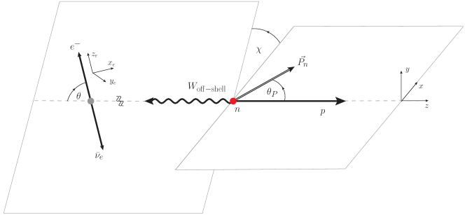
Figure 1: Definition of the polar angles $\theta$ and $\theta_{P}$, and the azimuthal angle $\chi$ describing the decay of a polarized neutron using the lepton pair as polarization analyzer. $\vec{P_{n}}$ denotes the polarization vector of the neutron which is chosen to lie in the $(x,z)$ plane. The components of the polarization vector of the electron $\vec{P}_{e}$ are defined in the right-handed $(x_{e},y_{e},z_{e})$ coordinate frame. The $y_{e}$–axis points into the page.

The angular decay distribution $W(\theta,\theta_{P},\chi)$ is determined by the master formula (see e.g. Ref. Kadeer:2005aq )

$$W(\theta,\theta_{P},\chi) \propto \sum_{\lambda_{e},\lambda_{W},\lambda^{\prime}_{W},J,J^{\prime},\lambda_{2}}\rho_{\lambda_{2}-\lambda_{W},\lambda_{2}-\lambda^{\prime}_{W}}(\theta_{P})(-1)^{J+J^{\prime}}|h_{\lambda_{e}\lambda_{\bar{\nu}}=1/2}|^{2}e^{-i(\lambda_{W}-\lambda^{\prime}_{W})\chi}$$ (14)

$$\times d^{J}_{\lambda_{W},\,\lambda_{e}-\lambda_{\bar{\nu}}}(\theta)d^{J^{\prime}}_{\lambda^{\prime}_{W},\,\lambda_{e}-\lambda_{\bar{\nu}}}(\theta)H_{\lambda_{2}\lambda_{W}}H^{*}_{\lambda_{2}\lambda^{\prime}_{W}},$$

where $\lambda_{\bar{\nu}}=1/2$ for the massless antineutrino and $\lambda_{e}=\pm 1/2$. In the configuration $\lambda_{e}=+1/2$ the electron helicity is flipped whereas the helicity is not flipped when $\lambda_{e}=-1/2$. The penalty factor for flipping the helicity of the electron is given by the ratio of the squares of the relevant leptonic flip and nonflip helicity amplitudes $|h_{\lambda_{e}=1/2\,\lambda_{\nu}=1/2}|^{2}/\,|h_{\lambda_{e}=-1/2\,\,\lambda_{\nu}=1/2}|^{2}=m_{e}^{2}/2q^{2}\,=:\,\delta_{e}$. The polarization of the neutron is described by the normalized density matrix

$$\rho_{\lambda_{1}\lambda_{1}^{{}^{\prime}}}(\theta_{P})=\frac{1}{2}\left(\begin{array}[]{cc}1+P_{n}\cos\theta_{P}&P_{n}\sin\theta_{P}\\ P_{n}\sin\theta_{P}&1-P_{n}\cos\theta_{P}\end{array}\right),$$ (15)

where $P_{n}$ denotes the magnitude of the polarization of the neutron. For completeness we list the Wigner small $d^{1}(\theta)$ function appearing in Eq. (14) which is given by

$$d^{1}_{mm^{\prime}}(\theta)=\left(\begin{array}[]{ccc}\frac{1}{2}(1+\cos\theta)&-\frac{1}{\sqrt{2}}\sin\theta&\frac{1}{2}(1-\cos\theta)\\ \frac{1}{\sqrt{2}}\sin\theta&\cos\theta&-\frac{1}{\sqrt{2}}\sin\theta\\ \frac{1}{2}(1-\cos\theta)&\frac{1}{\sqrt{2}}\sin\theta&\frac{1}{2}(1+\cos\theta)\end{array}\right)\vspace{0.1cm}$$ (16)

The rows and columns are labeled in the order of $(1,0,-1)$. The spin-0 Wigner function is simply $d^{0}_{00}(\theta)=1$.

The angles $\theta$, $\theta_{P}$ and $\chi$ are defined in Fig. 1. Fig. 1 provides a clear visualization of the two reference frames used in the cascade analysis. For once, there is the neutron rest frame which we will refer to as the $n$ frame, and second, one has the $W_{\rm off-shell}$ rest frame (or $(e^{-}\,\bar{\nu})$ center-of-mass frame) which will be referred to as the $q$ frame.

We mention that we have checked the correctness of the leptonic part of the angular decay distribution (14) given by

$${\cal L}_{\lambda_{W}\,\lambda^{\prime}_{W}}^{J\,J^{\prime}}(\lambda_{e})=|h_{\lambda_{e}\lambda_{\bar{\nu}}=1/2}|^{2}e^{-i(\lambda_{W}-\lambda^{\prime}_{W})\chi}d^{J}_{\lambda_{W},\,\lambda_{e}-\lambda_{\bar{\nu}}}(\theta)d^{J^{\prime}}_{\lambda^{\prime}_{W},\,\lambda_{e}-\lambda_{\bar{\nu}},}(\theta)$$ (17)

by an independent covariant calculation.

Putting in the correct normalization one obtains the four-fold decay distribution which we write as

$$\frac{d\Gamma_{\rm tot}}{dq^{2}d\cos\theta d\chi d\cos\theta_{P}}=\frac{1}{4\pi}\frac{\Gamma_{0}(q^{2}-m_{e}^{2})^{2}p}{M_{n}^{7}q^{2}}\Big{(}W(\theta)+P_{n}\cdot W^{P}(\theta,\theta_{P},\chi)\Big{)}\,,$$ (18)

where

$$\Gamma_{0}=\frac{G^{2}|V_{ud}|^{2}M_{n}^{5}}{192\pi^{3}}.$$ (19)

The momentum factor $p$ denotes the magnitude of the three-momentum of the proton or of the $W^{-}_{\rm off-shell}$ boson given by $p=\sqrt{Q_{+}Q_{-}}/2M_{n}$.

The $\cos\theta$-dependent unpolarized decay distribution $W(\theta)$ and the $(\theta,\theta_{P},\chi)$-dependent three-fold polarized angular decay distributions $W^{P}(\theta,\theta_{P},\chi)$ can be calculated from Eq. (14). One has

$$W(\theta) = \frac{3}{8}(1+\cos^{2}\theta)(|H_{\frac{1}{2}1}|^{2}+|H_{-\frac{1}{2}-1}|^{2})-\frac{3}{4}\cos\theta(|H_{\frac{1}{2}1}|^{2}-|H_{-\frac{1}{2}-1}|^{2})+\frac{3}{4}\sin^{2}\theta\Big{(}|H_{\frac{1}{2}0}|^{2}+|H_{-\frac{1}{2}0}|^{2}\Big{)}$$ (20)

$$+\frac{m_{e}^{2}}{2q^{2}}\bigg{\{}\frac{3}{2}(|H_{\frac{1}{2}t}|^{2}+|H_{-\frac{1}{2}t}|^{2})-3\cos\theta\,\mathop{\rm Re}\nolimits\left(H_{\frac{1}{2}t}H^{\ast}_{\frac{1}{2}0}+H_{-\frac{1}{2}t}H^{\ast}_{-\frac{1}{2}0}\right)$$

$$\qquad+\frac{3}{2}\cos^{2}\theta(|H_{\frac{1}{2}0}|^{2}+|H_{-\frac{1}{2}0}|^{2})+\frac{3}{4}\sin^{2}\theta(|H_{\frac{1}{2}1}|^{2}+|H_{-\frac{1}{2}-1}|^{2})\bigg{\}}$$

and

$$W^{P}(\theta,\theta_{P},\chi)\ =$$ (21)

$$\bigg{[}-\frac{3}{8}(1+\cos^{2}\theta)(|H_{\frac{1}{2}1}|^{2}-|H_{-\frac{1}{2}-1}|^{2})+\frac{3}{4}\cos\theta(|H_{\frac{1}{2}\,1}|^{2}+|H_{-\frac{1}{2}-1}|^{2})+\frac{3}{4}\sin^{2}\theta\Big{(}|H_{\frac{1}{2}0}|^{2}-|H_{-\frac{1}{2}0}|^{2}\Big{)}\bigg{]}\cos\theta_{P}$$

$$-\frac{3}{2\sqrt{2}}\sin\theta\sin\theta_{P}\bigg{[}\cos\chi\mathop{\rm Re}\nolimits\left(H_{\frac{1}{2}1}H^{*}_{\frac{1}{2}0}+H_{-\frac{1}{2}-1}H^{*}_{-\frac{1}{2}0}\right)+\sin\chi\mathop{\rm Im}\nolimits\left(H_{\frac{1}{2}1}H^{*}_{\frac{1}{2}0}-H_{-\frac{1}{2}-1}H^{*}_{-\frac{1}{2}0}\right)\bigg{]}$$

$$+\frac{3}{4\sqrt{2}}\sin 2\theta\sin\theta_{P}\bigg{[}\cos\chi\mathop{\rm Re}\nolimits\left(H_{\frac{1}{2}1}H^{*}_{\frac{1}{2}0}-H_{-\frac{1}{2}-1}H^{*}_{-\frac{1}{2}0}\right)+\sin\chi\mathop{\rm Im}\nolimits\left(H_{\frac{1}{2}1}H^{*}_{\frac{1}{2}0}+H_{-\frac{1}{2}-1}H^{*}_{-\frac{1}{2}0}\right)\bigg{]}$$

$$+\frac{m_{e}^{2}}{2q^{2}}\bigg{\{}\frac{3}{2}\cos\theta_{P}(|H_{\frac{1}{2}t}|^{2}-|H_{-\frac{1}{2}t}|^{2})-3\cos\theta\cos\theta_{P}\mathop{\rm Re}\nolimits\Big{(}H_{\frac{1}{2}t}H^{\ast}_{\frac{1}{2}0}-H_{-\frac{1}{2}t}H^{\ast}_{-\frac{1}{2}0}\Big{)}$$

$$\qquad+\frac{3}{2}\cos^{2}\theta\cos\theta_{P}\Big{(}|H_{\frac{1}{2}0}|^{2}-|H_{-\frac{1}{2}0}|^{2}\Big{)}-\frac{3}{4}\sin^{2}\theta\cos\theta_{P}(|H_{\frac{1}{2}1}|^{2}-|H_{-\frac{1}{2}-1}|^{2})$$

$$\qquad+\frac{3}{\sqrt{2}}\sin\theta\sin\theta_{P}\bigg{[}\cos\chi\,\mathop{\rm Re}\nolimits(H_{\frac{1}{2}1}H^{*}_{\frac{1}{2}t}-H_{-\frac{1}{2}-1}H^{*}_{-\frac{1}{2}t})+\sin\chi\,\mathop{\rm Im}\nolimits(H_{\frac{1}{2}1}H^{*}_{\frac{1}{2}t}+H_{-\frac{1}{2}-1}H^{*}_{-\frac{1}{2}t})\bigg{]}$$

$$\qquad-\frac{3}{2\sqrt{2}}\sin 2\theta\sin\theta_{P}\bigg{[}\cos\chi\,\mathop{\rm Re}\nolimits(H_{\frac{1}{2}1}H^{*}_{\frac{1}{2}0}-H_{-\frac{1}{2}-1}H^{*}_{-\frac{1}{2}0})+\sin\chi\,\mathop{\rm Im}\nolimits(H_{\frac{1}{2}1}H^{*}_{\frac{1}{2}0}+H_{-\frac{1}{2}-1}H^{*}_{-\frac{1}{2}0})\bigg{]}\bigg{\}},\qquad$$

where one has to remember to take the extra minus sign into account for the spin 0 - spin 1 interference contributions in Eq. (21) according to the factor $(-1)^{J+J^{\prime}}$. This factor arises from having used the Minkowski metric in the contraction of the lepton and hadron tensors (see e.g. Ref. Korner:1989ve ).

Figure 2: $q^{2}$ dependence of the partial flip and non-flip rates and the total rate

Let us briefly pause to discuss some kinematical aspects of the problem. The angle $\theta$ can be determined by measuring the energy $E_{e}$ of the electron in the neutron rest frame from the relation (see Sec. VII)

$$\cos\theta=\frac{1}{p(q^{2}-m_{e}^{2})}\Big{(}2q^{2}E_{e}-q_{0}(q^{2}+m_{e}^{2})\Big{)}.$$ (22)

This would require the knowledge of $q^{2}$, the value of which could be determined from a measurement of the energy or momentum of the recoiling proton. Barring hard photon emission from the neutron, proton or the $W_{\rm off-shell}$, the relevant relations are $E_{p}=(M_{n}^{2}+M_{p}^{2}-q^{2})/2M_{n}$ and $p=\sqrt{Q_{+}Q_{-}}/2M_{n}$. If the energy and/or the momentum of the proton cannot be measured, one can determine $q^{2}$ by inverting the relation $\cos\theta_{pe}=\cos\theta_{pe}(E_{e},q^{2})$ between the cosine of the opening angle of the proton and the electron in the $n$ frame and the kinematic variables $E_{e}$ and $q^{2}$ given by

$$\cos\theta_{pe}=M_{n}\frac{2E_{p}E_{e}-M_{n}(E_{p}+E_{e})+M_{p}^{2}+m_{e}^{2}}{\sqrt{Q_{+}Q_{-}}\,|\vec{p}_{e}|}.$$ (23)

In this case one would have to take care to properly treat the two solutions of the quadratic equation in $q^{2}$ that would result from inverting Eq. (23).

Returning to Eq. (21), one notes that the angular factors multiplying the imaginary parts of the helicity bilinears in Eq. (21) can be identified as $T$-odd triple momentum factors by writing

$$\sin\chi\sin\theta\sin\theta_{P} = -\hat{p}_{e}\cdot(\hat{s}_{n}\times\hat{p}_{p})$$

$$\sin\chi\sin 2\theta\sin\theta_{P} = -2\,\,\hat{p}_{e}\cdot(\hat{s}_{n}\times\hat{p}_{p})\,\hat{s}_{n}\cdot\hat{p}_{p}$$ (24)

where $\hat{s}_{n}$ is a unit vector in the direction of the polarization of the neutron and where the various unit three-vectors can be read-off from Fig. 1. In explicit form they read $\hat{p}_{p}=(0,0,1)$, $\hat{s}_{n}=(\sin\theta_{P},0,\cos\theta_{P})$ and $\hat{p}_{e}=-(\sin\theta\cos\chi,\sin\theta\sin\chi,\cos\theta)$. It is not difficult to see that the triple momentum product $\hat{p}_{e}\cdot(\hat{s}_{n}\times\hat{p}_{p})$ can be rewritten in the form $\hat{p}_{e}^{\prime}\cdot(\hat{s}_{n}\times\hat{p}_{\hat{\nu}}^{\prime})$ where the primed three-vectors refer to the corresponding three-vectors in the $n$ frame and where one has used three-momentum conservation in the $n$ frame $\hat{p}_{p}+\hat{p}_{e}^{\prime}+\hat{p}_{\hat{\nu}}^{\prime}=0$. The coefficient multiplying the triple product $\hat{p}_{e}^{\prime}\cdot(\hat{s}_{n}\times\hat{p}_{\hat{\nu}}^{\prime})$ is referred to as the $D$ term in the conventional three-body-decay approach. The associated $T$-odd observables can be fed by true $CP$-violating contributions or by $CP$-conserving electromagnetic rescattering corrections. In the Standard Model the $CP$-violating contributions in the $d\to u$ sector are of ${\cal O}(10^{-12})$ and are thus negligibly small Herczeg:1997se . The radiative rescattering corrections are also quite small. In the following we therefore assume that the form factors $F_{i}^{V/A}$ are relatively real and shall not further discuss the $T$-odd observables.

It is convenient and by now common practise to rewrite the angular decay distribution (18) in terms of the three Legendre polynomials $P_{0}(\cos\theta)=1$, $P_{1}(\cos\theta)=\cos\theta$ and $P_{2}(\cos\theta)=(3\cos^{2}\theta-1)/2$. One obtains

$$\frac{d\Gamma_{\rm tot}}{dq^{2}d\cos\theta d\cos\theta_{P}d\chi} = \frac{1}{8\pi}\Gamma_{0}\frac{(q^{2}-m_{e}^{2})^{2}p}{M_{n}^{7}q^{2}}\bigg{\{}{\cal H}_{\rm tot}(q^{2})+{\cal H}_{1}(q^{2})P_{1}(\cos\theta)+{\cal H}_{2}(q^{2})P_{2}(\cos\theta)$$ (25)

$$+P_{n}\,\cos\theta_{P}\Big{(}{\cal H}_{3}(q^{2})+{\cal H}_{4}(q^{2})P_{1}(\cos\theta)+{\cal H}_{5}(q^{2})P_{2}(\cos\theta)\Big{)}$$

$$+P_{n}\,\cos\chi\sin\theta_{P}\Big{(}\sin\theta\,{\cal H}_{6}(q^{2})+\sin 2\theta\,{\cal H}_{7}(q^{2})\Big{)}\,\bigg{\}},$$

where

$${\cal H}_{\rm tot}={\cal H}_{U}+{\cal H}_{L}+\delta_{e}(3{\cal H}_{S}+{\cal H}_{U}+{\cal H}_{L}).$$ (26)

The parity properties of the angular factors in Eq. (25) are determined by the parity transformations $\theta\to(\pi-\theta)$, $\theta_{P}\to(\pi-\theta_{P})$ and $\chi\to\chi+\pi$. The coefficients ${\cal H}_{i}(q^{2})$ multiplying the angular factors are linear superpositions of the helicity structure functions defined in Table 1. For the unpolarized case one has

$${\cal H}_{1}(q^{2}) = -\frac{3}{2}\Big{(}{\cal H}_{F}+4\,\delta_{e}{\cal H}_{SL_{+}}\Big{)},\qquad\quad\,\,\mbox{(p.v.)}$$

$${\cal H}_{2}(q^{2}) = \frac{1}{2}\left(1-2\,\delta_{e}\right)\Big{(}{\cal H}_{U}-2{\cal H}_{L}\Big{)},\qquad\mbox{(p.c.)}$$ (27)

and for the polarized case

$${\cal H}_{3}(q^{2}) = -\left(1+\,\delta_{e}\right)\left({\cal H}_{F}-{\cal H}_{L_{-}}\right)+3\,\delta_{e}{\cal H}_{S_{-}},\qquad\mbox{(p.v.)}$$

$${\cal H}_{4}(q^{2}) = \frac{3}{2}\left({\cal H}_{U}-4\,\delta_{e}{\cal H}_{SL_{-}}\right),\hskip 82.51282pt\mbox{(p.c.)}$$

$${\cal H}_{5}(q^{2}) = -\frac{1}{2}\left(1-2\,\delta_{e}\right)\left({\cal H}_{F}+2{\cal H}_{L_{-}}\right),\hskip 48.36958pt\mbox{(p.v.)}$$

$${\cal H}_{6}(q^{2}) = -\frac{3}{\sqrt{2}}\left({\cal H}_{LT_{+}}-2\,\delta_{e}{\cal H}_{ST_{-}}\right),\hskip 56.9055pt\mbox{(p.c.)}$$

$${\cal H}_{7}(q^{2}) = \frac{3}{2\sqrt{2}}\left(1-2\,\delta_{e}\right){\cal H}_{LT_{-}}.\hskip 82.51282pt\mbox{(p.v.)}$$ (28)

The parity properties of the helicity structure functions indicated in round brackets follow from the parity properties of the bilinear forms listed in Table 1.

Integrating the distribution (25) over the three angles $\theta$, $\theta_{P}$, and $\chi$ one obtains the total differential rate given by

$$\frac{d\Gamma_{\rm tot}}{dq^{2}}=\frac{\Gamma_{0}(q^{2}-m_{e}^{2})^{2}p}{M_{n}^{7}q^{2}}\,{\cal H}_{\rm tot}(q^{2}).$$ (29)

In analogy to Eq. (29) we define partial differential rates according to

$$\frac{d\Gamma_{i}}{dq^{2}}=\frac{\Gamma_{0}(q^{2}-m_{e}^{2})^{2}p}{M_{n}^{7}q^{2}}\,{\cal H}_{i}(q^{2}).$$ (30)

This leads to our final form of the angular decay distribution where we factor out the total differential rate from the curly bracket in Eq. (25). One has

$$\frac{d\Gamma_{\rm tot}}{dq^{2}d\cos\theta d\cos\theta_{P}d\chi} = \frac{1}{8\pi}\frac{d\Gamma_{\rm tot}}{dq^{2}}\bigg{\{}1+{\cal O}_{1}(q^{2})P_{1}(\cos\theta)+{\cal O}_{2}(q^{2})P_{2}(\cos\theta)$$ (31)

$$+P_{n}\,\cos\theta_{P}\Big{(}{\cal O}_{3}(q^{2})+{\cal O}_{4}(q^{2})P_{1}(\cos\theta)+{\cal O}_{5}(q^{2})P_{2}(\cos\theta)\Big{)}$$

$$+P_{n}\,\cos\chi\sin\theta_{P}\Big{(}\sin\theta\,{\cal O}_{6}(q^{2})+\sin 2\theta\,{\cal O}_{7}(q^{2})\Big{)}\,\bigg{\}},$$

where the normalized observables ${\cal O}_{i}(q^{2})$ are given by

$${\cal O}_{i}(q^{2})=\frac{{\cal H}_{i}(q^{2})}{{\cal H}_{\rm tot}(q^{2})}=\frac{d\Gamma_{i}\big{/}\,dq^{2}}{d\Gamma_{\rm tot}\big{/}\,dq^{2}}.$$ (32)

Next we discuss how to isolate the individual angular observables from the full decay distribution (25). There are three principal ways to do so. The most straightforward way is by a fit to the experimental angular decay distribution. A second possibility is to project out the observables by taking moments of the angular decay distribution w.r.t. appropiately chosen trigonometric functions as in Refs. Ivanov:2016qtw ; Blake:2017une . For example, the $\cos\theta$ dependent terms can be projected out by folding with Legendre polynomials. We follow a third method where one divides the angular phase space into different sectors and takes piece-wise sums and differences of the different sectors. This definition naturally leads to the set of frequently discussed asymmetry parameters.

The first observable ${\cal O}_{1}(q^{2})$ can be projected out by the standard forward–backward projection

$$A_{\rm FB}(q^{2})\ =\ \frac{1}{2}{\cal O}_{1}(q^{2}) = \frac{1}{d\Gamma_{\rm tot}/dq^{2}}\cdot\,\left(\int_{0}^{1}-\int_{-1}^{0}\right)d\cos\theta\int_{-1}^{1}d\cos\theta_{P}\int_{0}^{2\pi}d\chi\frac{d\Gamma_{\rm tot}}{dq^{2}d\cos\theta d\cos\theta_{P}d\chi}$$ (33)

$$= I_{1}(p.w.)\bigg{[}\left(\int_{0}^{1}-\int_{-1}^{0}\right)d\cos\theta\bigg{]},$$

where in the second row we have introduced a symbolic notation for the piece-wise (p.w.) integration described in the first row. The symbolic notation implies that the angular variables that do not appear in the symbolic-integration symbol are integrated over their full range. Using the symbolic notation one can project out the remaining observables in the angular decay distribution (25). One has

$$A_{\rm conv}(q^{2})\ =\frac{3}{8}{\cal O}_{2}(q^{2}) = I_{2}(p.w.)\bigg{[}\left(\int_{1/2}^{1}-\int_{0}^{1/2}-\int_{-1/2}^{0}+\int_{-1}^{-1/2}\right)d\cos\theta\bigg{]},$$

$$A_{\rm PFB}(q^{2})\ =\ P_{n}\cdot\frac{1}{2}{\cal O}_{3}(q^{2}) = I_{3}(p.w.)\bigg{[}\left(\int_{0}^{1}-\int_{-1}^{0}\right)d\cos\theta_{P}\bigg{]},$$

$$A_{\rm DFB}(q^{2})\ =\ P_{n}\cdot\frac{1}{4}{\cal O}_{4}(q^{2}) = I_{4}(p.w.)\bigg{[}\left(\int_{0}^{1}-\int_{-1}^{0}\right)d\cos\theta\bigg{]}\bigg{[}\left(\int_{0}^{1}-\int_{-1}^{0}\right)d\cos\theta_{P}\bigg{]},$$

$$A_{\rm Pconv}(q^{2})\ =\ P_{n}\cdot\frac{3}{16}{\cal O}_{5}(q^{2}) = I_{5}(p.w.)\bigg{[}\left(\int_{1/2}^{1}-\int_{0}^{1/2}-\int_{-1/2}^{0}+\int_{-1}^{-1/2}\right)d\cos\theta\bigg{]}\bigg{[}\left(\int_{0}^{1}-\int_{-1}^{0}\right)d\cos\theta_{P}\bigg{]},$$

$$A_{\chi_{1}(q^{2})}\ =\ P_{n}\cdot\frac{\pi}{8}{\cal O}_{6}(q^{2}) = I_{6}(p.w.)\bigg{[}2\left(\int_{0}^{\pi/2}-\int_{\pi/2}^{\pi}\right)d\chi\bigg{]},$$

$$A_{\chi_{2}}(q^{2})\ =\ P_{n}\cdot\frac{1}{3}{\cal O}_{7}(q^{2}) = I_{7}(p.w.)\bigg{[}\left(\int_{0}^{1}-\int_{-1}^{0}\right)d\cos\theta\bigg{]}\bigg{[}2\left(\int_{0}^{\pi/2}-\int_{\pi/2}^{\pi}\right)d\chi\bigg{]}.$$ (34)

We denote the two asymmetries $A_{\rm con}$ and $A_{\rm Pcon}$ associated with the square of $\cos\theta$ as the unpolarized and polarized convexity asymmetries because the respective angular decay distributions are described by a tilted upward or downward paraboloid depending on the sign of the corresponding coefficients ${\cal O}_{2}$ and ${\cal O}_{5}$. The convexity coefficients could also be isolated by taking the second derivative of the angular decay distribution w.r.t. $\cos\theta$.

Corresponding to the total and partial differential rates (29) and (30) we define integrated total and partial rates according to

$$\Gamma_{\rm tot}=\int_{m_{e}^{2}}^{(M_{n}^{2}-M_{p}^{2})}dq^{2}\frac{d\Gamma_{\rm tot}}{dq^{2}},\qquad\qquad\qquad\Gamma_{i}=\int_{m_{e}^{2}}^{(M_{n}^{2}-M_{p}^{2})}dq^{2}\frac{d\Gamma_{i}}{dq^{2}}.$$ (35)

This leads us to the definition of the average values of the observables $\langle{\cal O}_{i}\rangle$ which are the focus of the analysis in our paper. One has

$$\langle{\cal O}_{i}\rangle=\frac{\Gamma_{i}}{\Gamma_{\rm tot}}=\frac{\int_{m_{e}^{2}}^{(M_{n}^{2}-M_{p}^{2})}dq^{2}\,F(q^{2}){\cal H}_{i}(q^{2})}{\int_{m_{e}^{2}}^{(M_{n}^{2}-M_{p}^{2})}dq^{2}F(q^{2}){\cal H}_{\rm tot}(q^{2})},$$ (36)

where $F(q^{2})$ is a $q^{2}$-dependent phase-space factor given by $F(q^{2})=(q^{2}-m_{e}^{2})^{2}p/q^{2}$.

IV   Unpolarized neutron decays

We begin our discussion with the total differential rate given by

$$\frac{d\Gamma_{\rm tot}}{dq^{2}} = \frac{\Gamma_{0}(q^{2}-m_{e}^{2})^{2}p}{M_{n}^{7}q^{2}}\;\Bigg{[}{\cal H}_{U}+{\cal H}_{L}+\;\delta_{e}\;\Big{\{}3{\cal H}_{S}+{\cal H}_{U}+{\cal H}_{L}\Big{\}}\;\Bigg{]}\;.$$ (37)

As mentioned before the squared momentum transfer can be determined from the energy or momentum of the decay proton in the neutron rest frame. Note that ultracold neutrons (UCN) are practically at rest when they decay. They have typical velocities of 5 ms^-1 which corresponds to a kinetic energy of the neutron of $E_{e}^{\rm kin}=E_{e}-m_{n}=1.31\times 10^{-4}\mathop{\rm MeV}\nolimits$.

In Eq. (37) we have separated the helicity nonflip and helicity flip contributions where the last three terms in Eq. (37) muliplied by the helicity flip factor $\delta_{e}=m_{e}^{2}/(2q^{2})$ represent the helicity flip contribution. In Fig. 2 we present a plot of the $q^{2}$ dependence of the partial differential helicity nonflip rate $d\Gamma_{\rm nf}/dq^{2}$ and helicity flip rate $d\Gamma_{\rm hf}/dq^{2}$ as well as the sum of the two which is nothing but the total differential rate. The helicity flip contributions are negligibly small for $\ell=e,\mu$ in semileptonic bottom hadron decays and quite small (${\cal O}(1\,\%)$) for $\ell=\mu$ in semileptonic charm hadron decays. Contrary to this, the helicity flip contribution can obviously not be neglected in neutron $\beta$ decay. The helicity flip factor $\delta_{e}=m_{e}^{2}/(2q^{2})$ can become quite large close to threshold $q^{2}=m_{e}^{2}$. Numerically one has  $0.5\geq\delta_{e}\geq 0.07805$ and $0.7071\geq\sqrt{\delta_{e}}\geq 0.2794$. We have also listed the corresponding range of $\sqrt{\delta_{e}}$ which determines the flip suppression for the transverse polarization of the electron to be discussed later on. The total rate as well as the partial rates vanish at threshold $q^{2}=m_{e}^{2}$ (maximal recoil) and at zero recoil $q^{2}=(M_{n}-M_{p})^{2}$ due to the overall kinematical factors $(q^{2}-m^{2}_{e})^{2}$ and $p\sim((M_{n}-M_{p})^{2}-q^{2})^{1/2}$ in the rate expression (18). At zero recoil one has $d\Gamma_{\rm hf}/d\Gamma_{\rm nf}=(1+(F_{1}^{V}/F_{1}^{A})^{2})\delta_{e}(\rm z.r.)$ where the zero-recoil value of $\delta_{e}$ is $\delta_{e}(\rm z.r.)=0.078$ (see above). The total differential rate can be seen to be almost symmetrically distributed w.r.t. to its peak position at around $q^{2}=1\mathop{\rm MeV}\nolimits^{2}$.

The separation into helicity nonflip and flip contributions allows one to immediately conclude for the average longitudinal polarization of the electron in the $q$ frame along the electron’s momentum direction when one has integrated over the the three correlation angles $(\theta,\,\theta_{P},\,\chi)$. One has

$$P_{e}^{\ell}=\frac{d\Gamma_{\rm hf}-d\Gamma_{\rm nf}}{d\Gamma_{\rm hf}+d\Gamma_{\rm nf}},$$ (38)

since the helicity nonflip and flip rates correspond to the electron’s helicity values of $\lambda_{e}=-1/2$ and $\lambda_{e}=+1/2$, respectively. Close to threshold $q^{2}=m_{e}^{2}$ where the differential rates are small, the flip contribution is larger than the nonflip contribution in a narrow range of $q^{2}$ implying a small positive value of the longitudinal polarization of the electron, as can be seen in Fig. 3 where we plot the $q^{2}$ dependence of the longitudinal polarization of the electron. Starting at around $q^{2}=0.5\,{\rm MeV^{2}}$ the differential rate is dominated by the nonflip contribution such that the longitudinal polarization of the electron is negative in the remaining $q^{2}$ range as again evidenced in Fig. 3. The longitudinal polarization at zero recoil is determined by the flip/nonflip ratio at zero recoil calculated above which results in $P_{e}^{\ell}=-0.776$ at zero recoil in agreement with Fig. 3. The average value of the longitudinal polarization $\langle P_{e}^{\ell}\rangle\approx 0.50$ is close to the value of the polarization $P_{e}^{\ell}(q^{2})$ at the peak position of the differential rate at around $q^{2}\approx 1\mathop{\rm GeV}\nolimits^{2}$.

Figure 3: $q^{2}$ dependence of the longitudinal polarisation $P_{e}^{\ell}(q^{2})$ for two different sets of form factors (solid and dashed lines). The straight lines represent the longitudinal polarisation integrated over $q^{2}\in[m_{\ell}^{2},(M_{n}-M_{p})^{2}]$.

In Sec. VI we shall also present results on the transverse polarization of the decay electron.

Figure 4: Forward–backward asymmetry $A_{\rm FB}(q^{2})$ as a function of $q^{2}$ for two different sets of form factors (solid and dashed lines). The straight lines represent the average value forward–backward asymmetry integrated over $q^{2}\in[m_{\ell}^{2},(M_{n}-M_{p})^{2}]$.

In Fig. 4 we present a plot of the $q^{2}$ dependence of the forward–backward asymmetry $A_{\rm FB}(q^{2})$ where, according to Eq. (33), $A_{\rm FB}(q^{2})$ is given by

$$A_{\rm FB}(q^{2})=\frac{1}{2}\frac{{\cal H}_{1}(q^{2})}{{\cal H}_{\rm tot}(q^{2})}.$$ (39)

The forward–backward asymmetry starts with a rather large negative value $A_{\rm FB}(m_{e}^{2})=-0.46$ at threshold and goes to zero at zero recoil. The vanishing of the forward–backward asymmetry at zero recoil can be understood from the fact that ${\cal H}_{1}$ is proportional to $({\cal H}_{F}+4\delta_{e}{\cal H}_{SL_{+}})$. Both of these components vanish in the zero-recoil limit (see Eq. (13)).

If there is enough data and if the energy of the recoiling proton can be measured, it would certainly be interesting to take a detailed look at the $q^{2}$ dependence of the rate and the various polarization observables. In a more inclusive analysis one can also consider $q^{2}$-integrated quantities such as the total rate and the $q^{2}$ averages of the various polarization observables. It turns out that the $q^{2}$ integration of the rate and the polarization observables can be done analytically even including possible $q^{2}$ dependencies of the form factors. However, the resulting analytical expressions become quite long and unwieldy. A much more transparent and discerning representation of the integrated quantities can be obtained by performing a recoil expansion of the analytical results in terms of powers of the small parameter

$$\delta=(M_{n}-M_{p})/(M_{n}+M_{p})=0.689\cdot 10^{-3}.$$ (40)

In the recoil expansion it is convenient to split off an overall factor of $1/(1+\delta)^{8}$. We thus write

$$\Gamma_{i}=\frac{1}{(1+\delta)^{8}}\left(\Gamma_{i}^{(5)}\delta^{5}+\Gamma_{i}^{(6)}\delta^{6}+\ldots\right)$$ (41)

and formally call $\Gamma_{i}^{(5)}$, $\Gamma_{i}^{(6)}$ or common constant fractions of them the LO, NLO contributions in the recoil expansion.

In order to exhibit form factor effects and the linear contributions of the form factor $F^{A}_{3}$, the recoil expansion has to be done up to NNLO order, namely up to the order ${\cal O}(\delta^{7})$, where these contributions first appear. For the recoil expansion of the total rate one obtains

$$\Gamma\ =\ \frac{512\Gamma_{0}}{5(1+\delta)^{8}}\times\Big{[}\Big{\{}\left(3(F_{1}^{A})^{2}+(F_{1}^{V})^{2}\right)\,r(x)\Big{\}}\,\delta^{5}$$ (42)

$$\kern-12.0pt+\Big{\{}5F_{1}^{V}F_{3}^{V}x^{2}\left((2+13x^{2})\sqrt{1-x^{2}}+3x^{2}(4+x^{2})L_{2}\right)$$

$$-F_{1}^{A}F_{2}^{A}\left((8-26x^{2}+33x^{4})\sqrt{1-x^{2}}+15x^{6}L(x)\right)\Big{\}}\delta^{6}$$

$$\kern-12.0pt+\Big{\{}\frac{48}{7}(F_{2}^{A})^{2}(1-x^{2})^{7/2}$$

$$+2(F_{3}^{V})^{2}x^{2}\left((2-9x^{2}-8x^{4})\sqrt{1-x^{2}}-15x^{4}L(x)\right)$$

$$+F_{1}^{A}F_{2}^{A}\left((8-26x^{2}+33x^{4})\sqrt{1-x^{2}}+15x^{6}L(x)\right)$$

$$+\frac{1}{7}(3F_{1}^{V}+2F_{2}^{V})F_{2}^{V}\left((8-38x^{2}+87x^{4}+48x^{6})\sqrt{1-x^{2}}+105x^{6}L(x)\right)$$

$$-5F_{1}^{V}F_{3}^{V}x^{2}\left((2+13x^{2})\sqrt{1-x^{2}}+3x^{2}(4+x^{2})L(x)\right)$$

$$-F_{1}^{A}F_{3}^{A}x^{2}\left((6+83x^{2}+16x^{4})\sqrt{1-x^{2}}+15x^{2}(4+3x^{2})L(x)\right)$$

$$-\frac{1}{14}(F_{1}^{A})^{2}\left((30-69x^{2}+188x^{4}-44x^{6})\sqrt{1-x^{2}}+105x^{4}L(x)\right)$$

$$+\frac{3}{14}(F_{1}^{V})^{2}\left((2-27x^{2}-92x^{4}+12x^{6})\sqrt{1-x^{2}}-105x^{4}L(x)\right)$$

$$+\frac{2}{21}(F_{1}^{A})^{2}M_{n}^{2}\left((20-32x^{2}+319x^{4}+8x^{6})\sqrt{1-x^{2}}+105x^{4}(2+x^{2})L(x)\right)\langle(r_{1}^{A})^{2}\rangle$$

$$+\frac{2}{21}(F_{1}^{V})^{2}M_{n}^{2}\left((4+16x^{2}+271x^{4}+24x^{6})\sqrt{1-x^{2}}+105x^{4}(2+x^{2})L(x)\right)\langle(r_{1}^{V})^{2}\rangle\Big{\}}\,\delta^{7}+\ldots\Big{]}.\qquad$$

Since we assume the form factors to be relatively real, we use a simplified notation and write $(F_{1}^{A})^{2}=|F_{1}^{A}|^{2}$, $F_{1}^{A}\,F_{2}^{A}=\mathop{\rm Re}\nolimits(F_{1}^{A}F_{2}^{A\dagger})$ etc. in Eq. (42) and elsewhere. The LO ${\cal O}(\delta^{5})$ contribution has the familiar form proportional to $\left(3(F_{1}^{A})^{2}+(F_{1}^{V})^{2}\right)r(x)$ where ($r(0)=1$)

$$r(x)=\frac{1}{2}\left((2-9x^{2}-8x^{4})\sqrt{1-x^{2}}-15x^{4}\ln\left(\frac{1-\sqrt{1-x^{2}}}{x}\right)\right)=0.4726,$$ (43)

and where

$$x=m_{e}/(M_{n}-M_{p})=0.395\,.$$ (44)

It is quite remarkable that the electron mass dependence factors out in the LO term. If the second class form factor contributions are set to zero, the NLO contribution in the formal recoil expansion can be seen to vanish. This has been noted before in Refs. Kadeer:2005aq ; Chang:2014iba . The NLO contribution is again proportional to $\left(3(F_{1}^{A})^{2}+(F_{1}^{V})^{2}\right)r(x)$ in a formal sense if one expands $1/(1+\delta)^{8}=1-8\delta+\ldots$ .

As Eq. (42) shows, the factorization of the electron mass dependence is no longer true for the higher order terms in the recoil expansion. The higher order terms in Eq. (42) contain the logarithmic factor

$$L(x):=\ln\left(\frac{1-\sqrt{1-x^{2}}}{x}\right)=-1.580$$ (45)

which is always multiplied by powers of $x$ such that the $L(x)$ contribution vanishes in the zero electron mass limit.

In the literature the phase space factor needed for the total rate is usually obtained by first integrating over $E_{\nu}$ to obtain the $E_{e}$ spectrum followed by the integration over the $E_{e}$ spectrum. One obtains the well-known simple expressions only if one introduces zero recoil approximations in the integrand from the very beginning. Without zero recoil approximations the integration over $(E_{\nu},E_{e})$ phase space becomes quite complicated even in the unpolarized case (see Ref. Bender:1968zz and Ref. Wilkinson:1982hu Sec. 15.1) and is best done numerically. Compare this to our integration over the $(\cos\theta,q^{2})$ phase space which is quite straightforward because the phase-space integrations factorize. In addition, the first $\cos\theta$ integration is trivial. The $(\cos\theta,q^{2})$ integration route allows one to obtain compact expressions for the coefficients of the recoil expansion, as Eq. (42) shows. We emphasize that we do the zero recoil expansion after having done the full integration whereas in the $(E_{\nu},E_{e})$ phase space calculations the recoil expansion is frequently done prior to the last $E_{e}$ integration Wilkinson:1982hu which may lead to inaccurate results.

The contribution of the large induced pseudoscalar form factor $F_{3}^{A}$ sets in only at NNLO in the recoil expansion where it enters linearly. It is multiplied by the $x$-dependent factor

$$x^{2}\left((6+83x^{2}+16x^{4})\sqrt{1-x^{2}}+15x^{2}(4+3x^{2})L(x)\right)=0.193.$$ (46)

The accompanying relative recoil factor $\delta^{2}=0.475\cdot 10^{-6}$ reduces the linear ${\cal O}(\delta^{7})$ rate contribution of $F_{3}^{A}$ to an insignificant level. As it turns out, the same observation is true for the contribution of $F_{3}^{A}$ to all other partial rates.

In order to check on the sensitivity of the recoil expansion to the $q^{2}$ dependence of the form factors we have made a linear Ansatz for the form factors in terms of the isovector radii, i.e. we write

$$F_{i}^{X}(q^{2})=F_{i}^{X}(0)\left(1+\langle(r_{i}^{X})^{2}\rangle\frac{q^{2}}{6}\right)$$ (47)

for $i=1,2,3$; $X=V,A$. Eq. (42) shows that the form factor dependence of the form factors $F_{1}^{V/A}(q^{2})$ sets in only at NNLO while the form factor dependence of $F_{2,3}^{V/A}(q^{2})$ contributes only to higher orders in the recoil expansion. For the radii of the $F_{1}^{V}(q^{2})$ and $F_{1}^{A}(q^{2})$ form factors we take $\langle(r_{1}^{V})^{2}\rangle=0.66\,{\rm fm^{2}}=1.695\times 10^{-5}{\rm MeV^{-2}}$ and $\langle(r_{1}^{A})^{2}\rangle=0.45\,{\rm fm^{2}}=1.156\times 10^{-5}{\rm MeV^{-2}}$ Bourquin:1981ba ; Faessler:2008ix .

In order to be able to assess the importance of the $q^{2}$ dependence of the form factors in the ${\cal O}(\delta^{7})$ terms we take a closer numerical look at the first LO term and the last four ${\cal O}(\delta^{7})$ terms in Eq. (42). One has

$$\Gamma_{\rm tot} = \frac{512\Gamma_{0}\,\delta^{5}}{5(1+\delta)^{8}}\Big{[}\Big{\{}\Big{(}3(F_{1}^{A})^{2}+(F_{1}^{V})^{2}\Big{)}0.47\Big{\}}\ldots$$ (48)

$$-\Big{\{}\frac{1}{14}(F_{1}^{A})^{2}\Big{(}9.245-166.423\Big{)}+\frac{3}{14}(F_{1}^{V})^{2}\Big{(}12.782-22.623\Big{)}\Big{\}}\,\delta^{2}\,+\dots\Big{]},$$

where the numbers $166.423$ and $22.623$ refer to the $\langle(r_{1}^{A})^{2}\rangle$ and $\langle(r_{1}^{V})^{2}\rangle$ contributions. Eq. (48) shows that the $q^{2}$-dependent NNLO form factor contributions can become quite large compared to their $q^{2}$-independent NNLO counterparts. However, when multiplied by $\delta^{2}=0.475\cdot 10^{-6}$ the overall contribution of the $q^{2}$-dependent NNLO form factor contributions is insignificant. We have checked that this is true for all partial rates treated in this paper.

Returning to Eq. (42) one notes the remarkable result that the ${\cal O}(\delta^{6})$ term in the rate expansion vanishes altogether when the second class current contributions are set to zero, i.e. for $F_{3}^{V}=F_{2}^{A}=0$. The second class currents can be expected to be at most of ${\cal O}(\delta^{1})$, and thus the initial NLO ${\cal O}(\delta^{6})$ contribution of the second class form factors would be shifted up to the order ${\cal O}(\delta^{7})$. In fact, in a $SU(6)_{W}$ quark model calculation one finds $F_{3}^{V}\approx(M_{n}-M_{p})$ and $F_{2}^{A}=0$ Hussain:1990ai . The absence of NLO contributions in the recoil expansion of the rate implies that the NLO corrections to the $q^{2}$ average of an observable are entirely determined by the NLO correction to the partial rate associated with the observable.

This can be seen as follows. Consider the $q^{2}$ average $\langle{\cal O}_{i}\rangle$ of a given observable ${\cal O}_{i}$. In the recoil expansion one has

$$\langle{\cal O}_{i}\rangle=\frac{(\Gamma_{i}^{(5)}\,\delta^{5}+\Gamma_{i}^{(6)}\,\delta^{6}+\ldots)}{(\Gamma_{\rm tot}^{(5)}\,\delta^{5}+\Gamma_{\rm tot}^{(7)}\,\delta^{7}+\ldots)}=\frac{\Gamma_{i}^{(5)}}{\Gamma_{\rm tot}^{(5)}}\,\,\bigg{(}1+\Gamma_{i}^{(6)}/\Gamma_{i}^{(5)}\,\delta+\Big{(}\Gamma_{i}^{(7)}/\Gamma_{i}^{(5)}-\Gamma_{\rm tot}^{(7)}/\Gamma_{\rm tot}^{(5)}\Big{)}\,\delta^{2}+\ldots\bigg{)},$$ (49)

which shows that the NLO correction to $\langle{\cal O}_{i}\rangle$ is solely determined by the ratio $\Gamma_{i}^{(6)}/\Gamma_{i}^{(5)}$ when the contributions of the second class currents are set to zero. In Sec. VII we provide numerical results on the LO ratios $\Gamma_{i}^{(5)}/\Gamma_{\rm tot}^{(5)}$ as well as the NLO corrections $\Gamma_{i}^{(6)}/\Gamma_{i}^{(5)}$ for the various observables.

We now list the recoil expansion for the two unpolarized partial rates $\Gamma_{\rm FB}$ and $\Gamma_{\rm conv}$. One has

• p.v. partial forward–backward rate $\Gamma_{\rm FB}$  (${\cal H}_{\rm FB}=\frac{1}{2}\,{\cal H}_{1}=-\frac{3}{4}\,({\cal H}_{F}+4\delta_{e}{\cal H}_{SL_{+}}$)

  $$\Gamma_{\rm FB} = \frac{1}{2}\,\,\Gamma_{1}\ =\ \frac{64\Gamma_{0}}{(1+\delta)^{8}}\Big{[}3x^{2}((F_{1}^{V})^{2}+(F_{1}^{A})^{2})\left((1-x^{2})(5+x^{2})+4(1+2x^{2})\ln x\right)\delta^{5}$$ (50)

  $$+2\Big{(}(1-x^{2})\left((F_{1}^{V}+2F_{2}^{V})F_{1}^{A}(1-5x^{2}-2x^{4})-3(F_{1}^{V}F_{3}^{V}-F_{1}^{A}F_{2}^{A})x^{2}(1+5x^{2})\right)$$

  $$\qquad-12x^{4}\left((F_{1}^{V}+2F_{2}^{V})F_{1}^{A}+(F_{1}^{V}F_{3}^{V}-F_{1}^{A}F_{2}^{A})(2+x^{2})\right)\ln x\Big{)}\delta^{6}+O(\delta^{7})\Big{]}.$$

  The LO term in the recoil expansion can be seen to be entirely given by the longitudinal–scalar interference term $\delta_{e}{\cal H}_{SL_{+}}$ with the characteristic overall factor $x^{2}\sim m_{e}^{2}$. The parity-violating structure function ${\cal H}_{F}$ comes in only at NLO and is proportional to $(F_{1}^{V}+2F_{2}^{V})F_{1}^{A}$ when $F_{3}^{V}=F_{2}^{A}=0$.

• p.c. partial convexity rate $\Gamma_{\rm conv}$  (${\cal H}_{\rm conv}=\frac{3}{8}\,{\cal H}_{2}=\frac{3}{16}(1-2\delta_{e})({\cal H}_{U}-2{\cal H}_{L}$))
  For the integrated partial rate $\Gamma_{\rm conv}$ associated with the $\cos^{2}\theta$ contribution one obtains the recoil expansion

  $$\Gamma_{\rm conv} = \frac{3}{8}\Gamma_{2}\ =\ -\frac{24\Gamma_{0}}{5(1+\delta)^{8}}\Bigg{[}7\left((F_{1}^{V})^{2}+(F_{1}^{A})^{2}\right)\Bigg{(}(8+194x^{2}+113x^{4})\sqrt{1-x^{2}}$$ (51)

  $$\kern-24.0pt+15x^{2}(8+12x^{2}+x^{4})\,L(x)\Bigg{)}\delta^{5}-2\left(3(F_{1}^{V})^{2}+3(F_{1}^{A})^{2}+8(F_{2}^{V})^{2}+8(F_{2}^{A})^{2}\right)\times\kern-4.0pt$$

  $$\kern-12.0pt\times\Bigg{(}(4-40x^{2}-247x^{4}-32x^{6})\sqrt{1-x^{2}}-105x^{4}(2+x^{2})\,L(x)\Bigg{)}\delta^{7}+O(\delta^{8})\Bigg{]}.$$

  One notes that their are no NLO contributions to the p.c. partial rate $\Gamma_{\rm conv}$ when $F_{3}^{V}=F_{2}^{A}=0$.

V   Polarized neutron decays

With the availability of polarized neutron sources the number of possible correlation measurements in neutron $\beta$ decays is increased from two to seven as Eq. (25) shows. The neutron spin correlation measurements are proportional to the magnitude of the polarization of the neutron $P_{n}$, the value of which needs to be known to a high accuracy. Fortunately, one can presently avail of neutron beams with a very high degree of polarization close to 100$\%$ Surkau:1997 ; Kreuz:2005 ; Brown:2017mhw .

We now list the partial rates needed for the numerators of the five polarized obserables $\langle{\cal O}_{3}\rangle$ to $\langle{\cal O}_{7}\rangle$ where we include the respective projection factors from Eq. (III). The recoil expansion is carried out up to NLO. One obtains

• p.v. polarized forward–backward asymmetry $\Gamma_{\rm PFB}$  (${\cal H}_{\rm PFB}(q^{2})=\frac{1}{2}{\cal H}_{3}(q^{2})=-\frac{1}{2}(1+\delta_{e})({\cal H}_{F}-{\cal H}_{L_{-}})+\frac{3}{2}\delta_{e}{\cal H}_{S_{-}}$)

  $$\Gamma_{\rm PFB} = \frac{128\Gamma_{0}}{3(1+\delta)^{8}}\Big{[}3F_{1}^{V}F_{1}^{A}\left((1-x^{2})(1-5x^{2}-2x^{4})-12x^{4}\ln x\right)\delta^{5}$$ (52)

  $$-\Big{(}(1-x^{2})\left((2-7x^{2}+11x^{4})\left((F_{1}^{V}+2F_{2}^{V})F_{1}^{A}+F_{1}^{V}F_{2}^{A}\right)-9x^{2}(1+5x^{2})F_{3}^{V}F_{1}^{A}\right)$$

  $$\qquad+12x^{4}\left(x^{2}\left((F_{1}^{V}+2F_{2}^{V})F_{1}^{A}+F_{1}^{V}F_{2}^{A}\right)-3(2+x^{2})F_{1}^{A}F_{3}^{V}\right)\ln x\Big{)}\delta^{6}+O(\delta^{7})\Big{]}.$$

  For $F_{3}^{V}=F_{2}^{A}=0$ the axial form factor $F_{1}^{A}$ factors out and one arrives at the simple form

  $$\Gamma_{\rm PFB} = \frac{128\Gamma_{0}}{15(1+\delta)^{8}}\,F_{1}^{A}\Big{[}3F_{1}^{V}\left((1-x^{2})(1-5x^{2}-2x^{4})-12x^{4}\ln x\right)\delta^{5}$$ (53)

  $$+(F_{1}^{V}+2F_{2}^{V})\Big{(}2-9x^{2}+18x^{4}+x^{6}\Big{)}\delta^{6}+O(\delta^{7})\Big{]}$$

  The LO contribution agrees with the corresponding result of Ref. Gudkov:2008pf .

• p.c. double forward–backward asymmetry  (${\cal H}_{\rm DFB}(q^{2})=\frac{1}{4}{\cal H}_{4}(q^{2})=\frac{3}{8}({\cal H}_{U}-4\delta_{e}{\cal H}_{SL_{-}})$)

  $$\Gamma_{\rm DFB} = \frac{32\Gamma_{0}}{5(1+\delta)^{8}}\Bigg{[}F_{1}^{A}\Bigg{(}\left(5x^{2}(46+29x^{2})F_{1}^{V}-4(2-9x^{2}-8x^{4})F_{1}^{A}\right)\sqrt{1-x^{2}}$$ (54)

  $$\qquad+15x^{2}\left((8+16x^{2}+x^{4})F_{1}^{V}+4x^{2}F_{1}^{A}\right)\,L(x)\Bigg{)}\delta^{5}$$

  $$+4\Bigg{(}\left(5x^{2}(2+13x^{2})(F_{1}^{V}F_{2}^{A}-F_{3}^{V}F_{1}^{A})+4(2-9x^{2}-8x^{4})F_{1}^{A}F_{2}^{A}\right)\sqrt{1-x^{2}}$$

  $$\qquad+15x^{4}\left((4+x^{2})(F_{1}^{V}F_{2}^{A}-F_{3}^{V}F_{1}^{A})-4F_{1}^{A}F_{2}^{A}\right)L(x)\Bigg{)}\delta^{6}+O(\delta^{7})\Bigg{]}\,.$$

  The NLO contribution can be seen to vanish for $F_{3}^{V}=F_{2}^{A}=0$.

• p.v. polarized convexity parameter  (${\cal H}_{\rm Pconv}(q^{2})=\frac{3}{16}{\cal H}_{5}(q^{2})=-\frac{3}{32}(1-2\delta_{e})({\cal H}_{F}+2{\cal H}_{L_{-}})$)

  $$\Gamma_{\rm Pconv} = \frac{-16\Gamma_{0}}{(1+\delta)^{8}}\Big{[}3F_{1}^{V}F_{1}^{A}\left((1-x^{2})(1+10x^{2}+x^{4})+12x^{2}(1+x^{2})\ln x\right)\delta^{5}$$ (55)

  $$+\left((F_{1}^{V}+2F_{2}^{V})F_{1}^{A}-2F_{1}^{V}F_{2}^{A}\right)\Big{(}(1-x^{2})(1-8x^{2}-17x^{4})$$

  $$\qquad-12x^{4}(3+x^{2})\ln x\Big{)}\delta^{6}+O(\delta^{7})\Big{]}\,,$$

• p.c. azimuthal asymmetry 1  (${\cal H}_{\chi_{1}}(q^{2})=\frac{\pi}{8}{\cal H}_{6}(q^{2})=-\frac{3\pi}{8\sqrt{2}}({\cal H}_{LT_{+}}-2\delta_{e}{\cal H}_{ST_{-}})$)

  $$\Gamma_{\chi_{1}} = \frac{-4\pi\Gamma_{0}}{(1+\delta)^{8}}\bigg{[}2F_{1}^{A}\Big{(}x\sqrt{1-x^{2}}\left(4x^{2}(13+2x^{2})F_{1}^{V}-3(1+14x^{2})F_{1}^{A}\right)$$ (56)

  $$\qquad-3\left(4x^{2}(1+4x^{2})F_{1}^{V}+(1-8x^{2}-8x^{4})F_{1}^{A}\right)\arccos(x)\Big{)}\delta^{5}$$

  $$-\bigg{(}x\sqrt{1-x^{2}}\Big{(}(3+94x^{2}+8x^{4})F_{1}^{V}(F_{1}^{V}+2F_{2}^{V})-10x^{2}(11+10x^{2})(F_{1}^{V}+2F_{2}^{V})F_{1}^{A}$$

  $$\qquad\quad-2(9+74x^{2}-8x^{4})F_{1}^{A}F_{2}^{A}+16x^{2}(13+2x^{2})F_{1}^{V}F_{2}^{A}+12x^{2}(1+14x^{2})F_{3}^{V}F_{1}^{A}\Big{)}$$

  $$\qquad+3\Big{(}(1-12x^{2}-24x^{4})F_{1}^{V}(F_{1}^{V}+2F_{2}^{V})+2x^{2}(3+24x^{2}+8x^{4})(F_{1}^{V}+2F_{2}^{V})F_{1}^{A}$$

  $$\qquad\qquad-2(3-20x^{2}-8x^{4})F_{1}^{A}F_{2}^{A}-16x^{2}(1+4x^{2})F_{1}^{V}F_{2}^{A}$$

  $$\qquad\qquad+4x^{2}(1-8x^{2}-8x^{4})F_{3}^{V}F_{1}^{A}\Big{)}\arccos(x)\bigg{)}\delta^{6}+O(\delta^{7})\bigg{]},$$

• p.v. azimuthal asymmetry 2  (${\cal H}_{\chi_{2}}(q^{2})=\frac{1}{3}{\cal H}_{7}(q^{2})=\frac{1}{2\sqrt{2}}(1-2\delta_{e}){\cal H}_{LT_{-}}$)

  $$\Gamma_{\chi_{2}} = \frac{512\Gamma_{0}}{15(1+\delta)^{8}}(1-x)^{5}(1+5x)\Big{[}F_{1}^{V}F_{1}^{A}\delta^{5}$$

  $$+\left((F_{1}^{V}+2F_{2}^{V})F_{1}^{A}-2F_{1}^{V}F_{2}^{A}\right)\delta^{6}+O(\delta^{7})\Big{]}.$$

VI   Polarization of the decay electron

In Sec. IV we have already discussed some aspects of the longitudinal polarization of the decay electron. In this section we provide explicit LO and NLO expressions needed for the calculation of the average of the longitudinal polarization $\langle P_{e}^{\ell}\rangle$. We also extend the discussion to the transverse component of the decay electron. In all generality the two polarization components depend on the correlation angles $(\theta,\theta_{P},\chi)$. In this work we consider only averages of the two polarization components where the averaging is done w.r.t. the three correlation angles $(\theta,\theta_{P},\chi)$. This implies that we do not consider the correlation of the electron polarization with the neutron polarization as has been done e.g. in Ref. Nico:2009zua .

Using a slightly modified version of the master formula (14) one can calculate the differential $q^{2}$ distributions of the numerators of the relevant polarization expressions. One has

$$\frac{d\Gamma(P_{e}^{\ell})}{dq^{2}} = \frac{d\Gamma_{\rm hf}}{dq^{2}}-\frac{d\Gamma_{\rm nf}}{dq^{2}}\ =\ \frac{\Gamma_{0}(q^{2}-m_{e}^{2})^{2}p}{M_{n}^{7}q^{2}}\bigg{(}\delta_{e}\Big{(}3{\cal H}_{S}+{\cal H}_{U}+{\cal H}_{L}\Big{)}-\Big{(}{\cal H}_{U}+{\cal H}_{L}\Big{)}\bigg{)},\qquad\mbox{(p.c.)}$$ (58)

$$\frac{d\Gamma(P_{e}^{t})}{dq^{2}} = 2\frac{d\Gamma(\lambda_{e}=\tfrac{1}{2},\lambda^{\prime}_{e}=-\tfrac{1}{2})}{dq^{2}}\ =\ -\frac{3\pi}{4}\frac{\Gamma_{0}(q^{2}-m_{e}^{2})^{2}p}{M_{n}^{7}q^{2}}\sqrt{\frac{\delta_{e}}{2}}\Big{(}{\cal H}_{F}-2{\cal H}_{SL_{+}}\Big{)}.\qquad\qquad\mbox{(p.v.)}$$ (59)

The transverse polarization is proportional to the interference of the nonflip and flip helicity amplitudes and is thus proportional to the square root $\sqrt{\delta_{e}}$ of the helicity flip penalty factor. One needs to know the sign of the interference contribution which is given by

$$h_{\lambda_{e}=1/2\,\lambda_{\nu}=1/2}/\,h_{\lambda_{e}=-1/2\,\,\lambda_{\nu}=1/2}=\sqrt{m_{e}^{2}/2q^{2}}=\sqrt{\delta_{e}}.$$ (60)

The corresponding expressions for the two components of the polarization are given by

$$P_{e}^{\ell}=\frac{d\Gamma(P_{e}^{\ell})}{dq^{2}}\Big{/}\frac{d\Gamma_{\rm tot}}{dq^{2}}\qquad P_{e}^{t}=\frac{d\Gamma(P_{e}^{t})}{dq^{2}}\Big{/}\frac{d\Gamma_{\rm tot}}{dq^{2}}$$ (61)

As expected, the electron can be seen to be $100\,\%$ longitudinally polarized $P_{e}^{\ell}=-1$ in the limit of a vanishing electron mass, i.e. when setting $\delta_{e}=0$ in Eq. (58). In the same limit the transverse component vanishes as can again be seen by setting $\sqrt{\delta_{e}}=0$ in Eq. (59). In Fig. 5 we show a plot of the transverse polarization of the electron. The transverse polarization starts with a rather large positive value at threshold and then drops to zero at zero recoil. The vanishing at zero-recoil results from the fact that both ${\cal H}_{F}$ and ${\cal H}_{SL_{+}}$ vanish at zero recoil (see Eq. (13)). As in the case of the longitudinal polarization of the electron, the average value $\langle P_{e}^{t}\rangle\approx 0.45$ of the transverse polarization is close to the value of $P_{e}^{t}(q^{2})$ at the peak position of the differential total rate.

Next we integrate the numerators of the two polarization components in Eq. (61) over $q^{2}$ and expand the resulting expressions up to NLO in the recoil parameter $\delta$. One has

$$\Gamma(P_{e}^{\ell}) = -\frac{256\Gamma_{0}}{15(1+\delta)^{8}}\Bigg{\{}\Bigg{[}\left((F_{1}^{V})^{2}r(x)+(F_{1}^{A})^{2}r(x)\right)\Bigg{]}\delta^{5}$$ (62)

$$-6\Bigg{[}\left(5x^{2}(2+13x^{2})F_{1}^{V}F_{3}^{V}+(8-46x^{2}-97x^{4})F_{1}^{A}F_{2}^{A}\right)\sqrt{1-x^{2}}$$

$$\qquad+15x^{4}\left((4+x^{2})F_{1}^{V}F_{3}^{V}-(8+x^{2})F_{1}^{A}F_{2}^{A}\right)L(x)\Bigg{]}\delta^{6}+O(\delta^{7})\Bigg{\}},$$

$$\Gamma(P_{e}^{t}) = \frac{256\pi\Gamma_{0}}{(1+\delta)^{8}}x(1-x)^{4}\Bigg{\{}\left[(F_{1}^{V})^{2}+(F_{1}^{A})^{2}\right]\delta^{5}$$ (63)

$$+\frac{2}{5}(1+4x)\left[F_{1}^{V}F_{3}^{V}-F_{1}^{A}F_{2}^{A}+(F_{1}^{V}+2F_{2}^{V})F_{1}^{A}\right]\delta^{6}+O(\delta^{7})\Bigg{\}}.$$

It is important to realize that we define the two components of the polarization of the electron in the $q$ frame and not in the $n$ frame. The authors of Ref. Hagiwara:1989zt have shown how to convert the two polarization components from one frame to the other.

For completeness we present the numerator expression for the normal polarization of the electron which is given by

$$\frac{d\Gamma(P_{e}^{n})}{dq^{2}}=-\frac{3\pi}{2}\frac{\Gamma_{0}(q^{2}-m_{e}^{2})^{2}p}{M_{n}^{7}q^{2}}\sqrt{\frac{\delta_{e}}{2}}{\cal H}_{ISL_{+}}.$$ (64)

The normal polarization $P_{e}^{n}$ is a $T$-odd observable and is thus contributed to by the imaginary part of the bilinear helicity forms as shown in Eq. (64). The corresponding triple momentum product can be seen to be $(\hat{p}_{e}\times\hat{p}_{p})\cdot\hat{s}_{e}$.

Figure 5: Transverse polarisation of the electron as a function of $q^{2}$ for two different sets of form factors (solid and dashed lines). The straight lines represent the longitudinal polarisation integrated over $q^{2}\in[m_{\ell}^{2},(M_{n}-M_{p})^{2}]$.

VII   Electron energy distributions

One can turn the differential $\cos\theta$ distributions used in the cascade approach into differential $E_{e}$ distributions in the direct decay approach employing the relations

$$\cos\theta=\frac{2q^{2}E_{e}-q_{0}(q^{2}+m_{e}^{2})}{p(q^{2}-m_{e}^{2})}\,,\qquad\qquad d\cos\theta=dE_{e}\,\frac{2q^{2}}{p(q^{2}-m_{e}^{2})}$$ (65)

($q_{0}=(M_{n}^{2}-M_{p}^{2}+q^{2})/2M_{n}$), where $E_{e}$ is the energy of the electron in the $n$ frame ($m_{e}\leq E_{e}\leq(M_{n}^{2}-M_{p}^{2}+m_{e}^{2})/2M_{n}$). The first relation of Eq. (65) can be obtained by evaluating the scalar product $p_{n}\cdot p_{e}$ both in the $q$ frame and in the $n$ frame. The relevant four-vectors in the two frames read

$$\mbox{\rm$n$ frame}:\qquad p_{n}=(M_{n};0,0,0)\qquad\qquad\mbox{\rm$q$ frame}:\qquad p_{n}=M_{n}/\sqrt{q^{2}}\,(q_{0};0,0,p)$$ (66)

$$p_{e}=(E_{e};p_{e\,x},0,p_{e\,z})\qquad\qquad\qquad\qquad\ \ p_{e}=(\tilde{E}_{e};|\vec{\tilde{p}}_{e}|\sin\theta,-|\,\vec{\tilde{p}}_{e}|\cos\theta)$$

where $\tilde{E}_{e}=(q^{2}+m_{e}^{2})/2\sqrt{q^{2}}$ and $|\,\vec{\tilde{p}}_{e}|=(q^{2}-m_{e}^{2})/2\sqrt{q^{2}}$ are the energy and magnitude of the three-momentum of the electron in the $q$ frame. One then arrives at Eq. (65).

Next we consider the azimuthally integrated form of Eq. (25) and effect the change of variables given in Eq. (22). For the $(q^{2},E_{e})$ distribution one obtains

$$\frac{d\Gamma}{dq^{2}dE_{e}d\cos\theta_{P}} = \frac{\Gamma_{0}}{M_{n}^{7}}\Big{(}A_{0}(q^{2},m_{e})+A_{1}(q^{2},m_{e})E_{e}+A_{2}(q^{2})E_{e}^{2}$$ (67)

$$+P_{n}\cos\theta_{P}\left(A_{0}^{P}(q^{2},m_{e})+A_{1}^{P}(q^{2},m_{e})E_{e}+A_{2}^{P}(q^{2})E_{e}^{2}\right)\Big{)}\,.$$

Quite remarkably, the coefficients of the quadratic energy dependence $A_{2}(q^{2})$ and $A_{2}^{P}(q^{2})$ depend only on $q^{2}$ and not on the mass $m_{e}$ of the lepton Penalva:2019rgt . For these two coefficients one finds

$$A_{2}(q^{2}) = \,\frac{3q^{2}}{2p^{2}}({\cal H}_{U}-2{\cal H}_{L})\,,$$

$$A_{2}^{P}(q^{2}) = -\,\frac{3q^{2}}{2p^{2}}({\cal H}_{F}+2{\cal H}_{L_{-}})\,.$$ (68)

An explicit calculation shows that $({\cal H}_{F}+2{\cal H}_{L_{-}})\sim p^{2}$ which will compensate the $p^{2}$ factor in the denominator of the polarized term $A_{2}^{P}(q^{2})$ in Eq. (VII). The unpolarized term $A_{2}(q^{2})$ proportional to $({\cal H}_{U}-2{\cal H}_{L})\sim p^{3}$ even vanishes at the zero recoil point $q^{2}=(M_{n}-M_{p})^{2}$ and $E_{e}=((M_{n}-M_{p})^{2}+m_{e}^{2})/(2(M_{n}-M_{p}))$.

The remaining coefficients in (67) are given by

$$A_{0}(q^{2},m_{e}) = \frac{3}{8q^{2}p^{2}}\Big{(}q^{2}(q^{2}+m_{e}^{2})(2p^{2}+q^{2}+m_{e}^{2})\left({\cal H}_{U}-2{\cal H}_{L}\right)$$

$$+2p^{2}(q^{2}-m_{e}^{2})\left((2q^{2}+m_{e}^{2}){\cal H}_{L}+m_{e}^{2}{\cal H}_{S}\right)+2q_{0}p(q^{2}+m_{e}^{2})\left(q^{2}{\cal H}_{F}+2m_{e}^{2}{\cal H}_{SL+}\right)\Big{)}\,,$$

$$A_{1}(q^{2},m_{e}) = \frac{-3}{2p^{2}}\Big{(}q_{0}(q^{2}+m_{e}^{2})\left({\cal H}_{U}-2{\cal H}_{L}\right)+p\left(q^{2}{\cal H}_{F}+2m_{e}^{2}{\cal H}_{SL+}\right)\Big{)}\,,$$

$$A_{0}^{P}(q^{2},m_{e}) = \frac{-3}{8q^{2}p^{2}}\Big{(}q^{2}(q^{2}+m_{e}^{2})(2p^{2}+q^{2}+m_{e}^{2})\left({\cal H}_{F}+2{\cal H}_{L-}\right)$$

$$-2p^{2}(q^{2}-m_{e}^{2})\left((2q^{2}+m_{e}^{2}){\cal H}_{L-}+m_{e}^{2}{\cal H}_{S-}\right)+2q_{0}p(q^{2}+m_{e}^{2})\left(q^{2}{\cal H}_{U}-2m_{e}^{2}{\cal H}_{SL-}\right)\Big{)}\,,$$

$$A_{1}^{P}(q^{2},m_{e}) = \frac{3}{2p^{2}}\Big{(}q_{0}(q^{2}+m_{e}^{2})\left({\cal H}_{F}+2{\cal H}_{L-}\right)+p\left(q^{2}{\cal H}_{U}-2m_{e}^{2}{\cal H}_{SL-}\right)\Big{)}\,.\qquad$$ (69)

The two-fold distribution (67) can be further integrated over $q^{2}$ or $E_{e}$ where the respective limits of integration can be derived from Eq. (22) by setting $\cos\theta=\pm 1$. They read

$$E_{e}^{\pm}=\frac{1}{2q^{2}}\Big{(}q_{0}(q^{2}+m_{e}^{2})\pm p(q^{2}-m_{e}^{2})\Big{)}$$ (70)

and

$$q^{2}_{\pm} = \frac{M_{n}(M_{n}^{2}-M_{p}^{2}+m_{e}^{2}-2M_{n}E_{e})\Big{(}E_{e}\pm\sqrt{E_{e}^{2}-m_{e}^{2}}\Big{)}}{M_{n}^{2}+m_{e}^{2}-2M_{n}E_{e}}$$ (71)

$$= \frac{2M_{n}^{2}}{2M_{n}(E_{e}^{\rm max}-E_{e})+M_{p}^{2}}\left((E_{e}^{\rm max}-E_{e})\bigg{(}E_{e}\pm\sqrt{E_{e}^{2}-m_{e}^{2}}\,\,\bigg{)}+\frac{m_{e}^{2}M_{p}^{2}}{2M_{n}^{2}}\right)\,,$$

where $E_{e}^{\rm max}=(M_{n}^{2}-M_{p}^{2}+m_{e}^{2})/2M_{n}$. Integrating the distribution (67) over $E_{e}$ in the limits (70) one obtains the one-fold $q^{2}$ distribution discussed in Sec. III. On the other hand, integrating (67) over $q^{2}$ in the limits (71) one obtains the one-fold $E_{e}$ distribution discussed in Refs. Bender:1968zz ; Wilkinson:1982hu for the unpolarized case.

VIII   Numerical results

Observable	LO result	full result	LO value	$\delta_{i}$(NLO)	$\langle A_{i}\rangle^{\prime}/\langle A_{i}\rangle$ (LO)
$\langle A_{\rm FB}\rangle$	$\left(|F_{1}^{A}|^{2}+|F_{1}^{V}|^{2}\right)r_{1}(x)/R(x)$	$-0.1440$	$-0.1448$	$-5.35\,\text{\textperthousand}$	$-0.332$
$\langle A_{\rm conv}\rangle$	$\left((F_{1}^{A})^{2}+(F_{1}^{V})^{2}\right)r_{2}(x)/R(x)$	$-0.04771$	$-0.04771$	$0\,\text{\textperthousand}$	$-0.332$
$\langle A_{\rm PFB}\rangle/P_{n}$	$F_{1}^{V}F_{1}^{A}\,r_{3}(x)/R(x)$	$+0.2382$	$+0.2388$	$-2.47\,\text{\textperthousand}$	$-0.518$
$\langle A_{\rm DFB}\rangle/P_{n}$	$\left(|F_{1}^{A}|^{2}\,r_{4}(x)+F_{1}^{V}F_{1}^{A}\,r_{4^{\prime}}(x)\right)/R(x)$	$-0.2159$	$-0.2159$	$0\,\text{\textperthousand}$	$-0.145$
$\langle A_{\rm Pconv}\rangle/P_{n}$	$F_{1}^{V}F_{1}^{A}\,r_{5}(x)/R(x)$	$-0.03686$	$-0.03679$	$+1.88\,\text{\textperthousand}$	$-0.518$
$\langle A_{\chi_{1}}\rangle/P_{n}$	$\pi\left(|F_{1}^{A}|^{2}\,r_{6}(x)+F_{1}^{V}F_{1}^{A}\,r_{6}^{\prime}(x)\right)/R(x)$	$+0.3351$	$+0.3348$	$+0.85\,\text{\textperthousand}$	$+0.129$
$\langle{A}_{\chi_{2}}\rangle/P_{n}$	$F_{1}^{V}F_{1}^{A}\,r_{7}(x)/R(x)$	$+0.03705$	$+0.03693$	$+3.24\,\text{\textperthousand}$	$-0.518$
$\langle P_{e}^{\ell}\rangle$	$\left(|F_{1}^{A}|^{2}r_{8}(x)+|F_{1}^{V}|^{2}r_{8}^{\prime}(x)\right)/R(x)$	$-0.4964$	$-0.4964$	$0\,\text{\textperthousand}$	$+0.337$
$\langle P_{e}^{t}\rangle$	$\pi$ $(|F_{1}^{A}|^{2}+|F_{1}^{V}|^{2})r_{9}(x)/R(x)$	$+0.3937$	$+0.3931$	$+1.63\,\text{\textperthousand}$	$-0.332$

Table 2: Asymmetries in neutron $\beta$ decay. First column: Asymmetry; Second column: Analytical expression for LO result $\Gamma_{i}^{(5)}/\Gamma^{(5)}$; Third column: Full result; Fourth column: numerical value of the LO result; Fifth column: numerical value for the relative NLO correction; Sixth column: error propagation factor.

In Table 2 we list our analytical and numerical results for the nine average asymmetries calculated in this paper where we include the two polarization components of the electron in the list of the asymmetries since the polarization components are frequently referred to as polarization asymmetries in the literature. In order to simplify the discussion we set $P_{n}=1$ for the five polarization observables, i.e. we set $\langle A_{i}\rangle/P_{n}=\langle A_{i}\rangle$ for the five polarization observables $\langle A_{\rm PFB}\rangle$ to $\langle A_{\chi_{2}}\rangle$.

Column 2 contains our analytical LO results for the average asymmetries $\langle A_{i}\rangle=P_{i}\,\langle{\cal O}_{i}\rangle=P_{i}\,\Gamma_{i}^{(5)}/\Gamma^{(5)}$ where the factors $P_{i}$ are the same as in Eqs. (33) and (III), $P_{\ell}=P_{t}=1$. We have cancelled some numerical factors in the ratio expressions which are now normalized to the rate factor

$$R(x)=\left(3(F_{1}^{A})^{2}+(F_{1}^{V})^{2}\right)r(x),$$ (72)

where $r(x)$ is listed in Eq. (43). The LO contributions in column 2 are written in terms of a number of $x$-dependent functions $r_{1}(x)$ to $r_{9}(x)$ which are defined by

$$r_{1}(x) = \frac{15}{8}x^{2}\left[(1-x^{2})(5+x^{2})+4(1+2x^{2})\ln x\right]\ =\ -0.1531,$$

$$r_{2}(x) = -\frac{3}{64}\left[\sqrt{1-x^{2}}\left(8+194x^{2}+113x^{4}\right)+15x^{2}\left(8+12x^{2}+x^{4}\right)L(x)\right]\ =\ -0.05042,$$

$$r_{3}(x) = \frac{5}{4}\left[\left(1-x^{2}\right)\left(1-5x^{2}-2x^{4}\right)-12x^{4}\ln x\right]\ =\ 0.5196,$$

$$r_{4}(x) = -\frac{1}{2}r(x)\ =\ -0.2363,$$

$$r_{4}^{\prime}(x) = \frac{5}{16}x^{2}\left[\sqrt{1-x^{2}}\left(46+29x^{2}\right)+3\left(8+16x^{2}+x^{4}\right)L(x)\right]\ =\ -0.1691,$$

$$r_{5}(x) = -\frac{15}{32}\left[\left(1-x^{2}\right)\left(1+10x^{2}+x^{4}\right)+12x^{2}(1+x^{2})\ln x\right]\ =\ -0.08004,$$

$$r_{6}(x) = \frac{15}{64}\left[x\sqrt{1-x^{2}}\left(1+14x^{2}\right)+\left(1-8x^{2}-8x^{4}\right)\arccos x\right]\ =\ 0.1498,$$

$$r_{6}^{\prime}(x) = -\frac{5}{16}x^{2}\left[x\sqrt{1-x^{2}}\left(13+2x^{2}\right)-3\left(1+4x^{2}\right)\arccos x\right]\ =\ 0.04116,$$

$$r_{7}(x) = \frac{1}{3}(1-x)^{5}(1+5x)\ =\ 0.08033,$$

$$r_{8}(x) = -\frac{1}{6}\left[\sqrt{1-x^{2}}\left(18+139x^{2}+8x^{4}\right)+15x^{2}\left(8+3x^{2}\right)L(x)\right]\ =\ -0.8855,$$

$$r_{8}^{\prime}(x) = -\frac{1}{6}\left[\sqrt{1-x^{2}}\left(6+193x^{2}+56x^{4}\right)+15x^{2}\left(8+9x^{2}\right)L(x)\right]\ =\ 0.05966,$$

$$r_{9}(x) = \frac{5}{2}x(1-x)^{4}\ =\ 0.1322.$$ (73)

In column 3 we list numerical values for the full results using the form factor values specified in Eqs. (9) and (10). The full values are calculated prior to the expansion in $\delta$, not taking into account the $q^{2}$ dependence of the form factors. This $q^{2}$ dependence of the form factors effects the result far below the precision given in Tab. 2. The predicted values for the average asymmetries range from $\langle{A}_{\chi_{2}}\rangle=0.03705$ to $\langle{P}_{e}^{\ell}\rangle=-0.4964$. The small value of $\langle{A}_{\chi_{2}}\rangle=0.03705$ results in part from the smallness of the sector projection factor $P_{{A}_{\chi_{2}}}=1/3$. In column 4 we write down the LO numerical values of the analytical LO results in column 3. The LO values can be seen to be quite close to the full results.

In order to check on the magnitude of the NLO corrections we list the numerical values for the relative NLO corrections $\delta_{i}$(NLO) im column 4. According to Eq. (49) the NLO corrections are given by $\delta_{i}({\rm NLO})=\Gamma_{i}^{(6)}/\Gamma_{i}^{(5)}\,\delta$. The analytical expressions for the NLO corrections can be found in Eqs. (50–• ‣ V) and Eqs. (62–63) and have been evaluated with the form factor values listed in Eqs. (9) and (10). The NLO corrections to the LO results listed in column 5 are generally quite small or even zero. The largest NLO correction occurs for the forward–backward asymmetry $\langle F_{\rm FB}\rangle$ with $\delta_{\rm FB}({\rm NLO})=-5.35\,\text{\textperthousand}$. The NLO corrections move the LO values very close to the full result in column 3 which shows that one can safely truncate the recoil expansion at NLO.

Our results on the polarization observable $\langle A_{\rm PFB}\rangle$ can be directly compared to the experiment since the average asymmetry $\langle A_{\rm PFB}\rangle$ is identical to the so-called proton asymmetry parameter $C$ in the conventional approach. The parameter $C$ has been measured by the PERKEO II collaboration with the result $C=-0.2377(26)$ Schumann:2007hz . This value is quite compatible with our full result $\langle A_{\rm PFB}\rangle=C=-0.2382$. The relative NLO correction $\delta_{i}\,({\rm NLO})=-2.47\,\text{\textperthousand}$ shifts the LO result $\langle A_{\rm PFB}\rangle({\rm LO})=0.2328$ close to the central experimental value.

It is interesting to know how an error in the value of the axial form factor propagates to the average asymmetries. This bears on the question on how accurately can one determine the value of the axial form factor from a measurement of the average asymmetries discussed in this paper. We discuss this issue using the usual ratio $\lambda=F_{1}^{A}/F_{1}^{V}$. Expanding the asymmetry around the central value $\lambda=1.2724$ from Ref. Tanabashi:2018oca , one has

$$\langle A_{i}\rangle(\lambda+\Delta\lambda)=\langle A_{i}\rangle(\lambda)\Big{(}1+\frac{\langle A_{i}\rangle^{\prime}(\lambda)}{\langle A_{i}\rangle(\lambda)}\cdot\Delta\lambda\Big{)}.$$ (74)

The experimental value of $\Delta\lambda=0.0023$ Tanabashi:2018oca is small enough that we can terminate the Taylor expansion after the linear term. The relative error of the average asymmetry $\langle A_{i}\rangle$ is given by $\delta\langle A_{i}\rangle=\langle A_{i}\rangle^{\prime}(\lambda)/\langle A_{i}\rangle(\lambda)\cdot\Delta\lambda$. The ratio

$$\frac{\delta\langle A_{i}\rangle}{\Delta\lambda}=\frac{\langle A_{i}\rangle^{\prime}(\lambda)}{\langle A_{i}\rangle(\lambda)}$$ (75)

provides a measure of the error propagation from the absolute error of $\lambda$ to the relative error of the asymmetry $\langle A_{i}\rangle(\lambda)$. One wants the error propagation factor to be as large as possible. Of course, one can turn this argument around. The error propagation from the the relative error of the asymmetry $\langle A_{i}\rangle(\lambda)$ to the absolute error of $\lambda$ is given by the inverse of Eq. (75). A good asymmetry measurement is characterized by a small value of the inverse of Eq. (75). In column 6 we have listed the LO values of the ratio $\langle A_{i}\rangle^{\prime}(\lambda)/\langle A_{i}\rangle(\lambda)$ where we take the central PDG value $\lambda=1.2724$. The error propagation factor ranges from $0.129$ for $\langle A_{\chi_{1}}\rangle$ to $0.518$ for $\langle A_{\rm PFB}\rangle,\,\langle A_{\rm Pconv}\rangle$ and $\langle A_{\chi_{2}}\rangle$. The latter three asymmetries are thus the best candidates for an accurate measurement of the axial form factor $F_{1}^{A}$. These three asymmetries would have to be measured with an error less than $1.19\,\text{\textperthousand}$ to reduce the present PDG error on $\lambda$ given by $2.3\,\text{\textperthousand}$.

It is interesting to compare the error propagation of $\lambda$ into the total rate where one has $\Gamma^{\prime}(\lambda)/\Gamma(\lambda)=6\lambda/((1+3\lambda^{2})=1.303$. As concerns the error propagation, the rate measurement is $2.5$ times better than the best asymmetry measurement. However, the extraction of $\lambda$ from the rate measurement requires additional input in the form of the value of $V_{ud}$ and the size of the radiative corrections Czarnecki:2019mwq . In contrast to this the asymmetry measurements are independent of the value of $V_{ud}$. Furthermore, the bulk of the radiative corrections can be expected to cancel out in the asymmetry ratios.

IX   Summary and conclusion

We have presented the results of a detailed analysis of unpolarized and polarized neutron $\beta$ decays in the helicity framework. We have derived exact relativistic formulas for the $q^{2}$ distribution of the total rate and the partial correlation rates without employing any recoil approximations. The $q^{2}$ integration of the differential rates was done analytically, and the results were checked by numerical integration. After the $q^{2}$ integration we performed an expansion in the small recoil parameter $\delta=(M_{n}-M_{p})/(M_{n}+M_{p})=0.689\cdot 10^{-3}$, the series of which has very rapid convergence properties. Doing the recoil expansion after the integration spares one from having to guess to which order a given term will contribute to the final result before doing the final integration. We found that the NLO term in the recoil expansion vanish for three of the four p.c. observables analyzed in this paper. These are $\langle A_{\rm conv}\rangle$, $\langle A_{\rm DFB}\rangle$ and the average value of the longitudinal polarization $P_{e}^{\ell}$ of the electron.

At the LO of the recoil expansion one has contributions only from the form factors $F_{1}^{V}$ and $F_{1}^{A}$. This opens the opportunity for further measurements of the form factor $F_{1}^{A}$ from other observables on top of the usual determination of $F_{1}^{A}$ from the rate measurement (see the discussion in Ref. Czarnecki:2018okw ; Czarnecki:2019mwq ). Particularly well suited for such a measurement of $F_{1}^{A}$ would be the three observables $\langle A_{\rm PFB}\rangle$, $\langle A_{\rm Pconv}\rangle$ and $\langle A_{\chi_{2}}\rangle$ which are the most sensitive asymmetries for a determination of $F_{1}^{A}$. We find that there is no possibility to measure the value of the form factor $F_{3}^{A}$ nor the slope of the form factors $F_{1}^{V}(q^{2})$ or $F_{1}^{V}(q^{2})$ close to origin since both contribute only to higher orders in the recoil expansion.

Some of our results are directly applicable to results derived in the conventional three-body decay analysis done in the $n$ frame. Very obviously, this holds true for the total rate and the spin–momentum correlation between the spin of the neutron and the momentum of the proton conventionally called the spin–proton correlation parameter $C$. The spin–electron and spin–neutrino correlations defined in the conventional approach are not directly related to the corresponding correlations in the helicity approach. As concerns azimuthal correlations one can choose the momentum of the proton to define the $z$ axis in the direct decay approach (system 2 in Ref. Korner:1998nc ). For this choice the azimuthal correlations in the two approaches are simply related. As shown in Sec. III, the $T$-odd triple correlation parameter $D$ of the conventional approach is proportional to $(-1/2\,{\cal H}_{ILT_{-}}+\delta_{e}{\cal H}_{IST_{+}})$ in the helicity approach. The same holds true for the $T$-odd normal polarization $P_{e}^{n}$ of the electron discussed in Sec. VII.

As discussed in Sec. VII, one can turn the differential $\cos\theta$ distribution used in the helicity approach into a differential electron energy distribution in the conventional direct decay approach employing the relation (22),

$$\cos\theta=\frac{2q^{2}E_{e}-q_{0}(q^{2}+m_{e}^{2})}{p(q^{2}-m_{e}^{2})}\,,$$ (76)

where $E_{e}$ is the energy of the electron in the neutron rest frame.

Other results of the conventional three-body decay analysis such as opening angle distributions between pairs of the three final state particles $(p,\,e^{-},\,\bar{\nu})$ in the neutron rest frame are not part of the helicity analysis. These distributions can be obtained by applying the appropiate boosts to the helicity distributions either analytically or by Monte Carlo event generation methods as has been done in the analysis of polarized hyperon decays $\Xi^{0}\to\Sigma^{+}+\ell^{-}+\bar{\nu}_{\ell}\,\,(\ell^{-}=e^{-},\,\mu^{-})$ in Ref. Kadeer:2005aq .

One of the advantages of using normalized angular observables is that they do not depend on the value of $|V_{ud}|$ which is welcome even if the relative error on $|V_{ud}|$ is small ($\sim$ $0.1$‰ Tanabashi:2018oca ). Furthermore, the bulk of the radiative corrections can be expected to cancel when taking ratios of rates since large parts of the radiative corrections are proportional to the Born term rates.

In this paper we have restricted our discussion to the helicity analysis of free neutron $\beta$ decays. There is no obstacle to also apply the helicity method to nuclear $\beta$ decays.

The results of this paper can also be formulated in terms of an effective field theory (EFT) approach (see e.g. Ref. Gonzalez-Alonso:2018omy ). In addition, New Physics effects (see e.g. Ref. Cirgiliano:2019nyn ) are easily incorporated into the helicity framework. An EFT helicity approach to neutron $\beta$ decay including New Physics effects will be the subject of a sequel to this paper.

Acknowledgments

We would like to thank J. Erler, W. Heil, D. McKay, W. Shepherd for discussions and encouragement. B.M. has been supported by the European Union through the European Regional Development Fund – the Competitiveness and Cohesion Operational Programme (KK.01.1.1.06). B.M. would like to acknowledge the support of the Alexander von Humboldt foundation as well as the hospitality of the theory group THEP at the Institute of Physics at the Johannes Gutenberg University. The research of S.G. was supported by the European Regional Development Fund under Grant No. TK133. S.G. also acknowledges support from the PRISMA and PRISMA⁺ (project No. 2118 and ID 39083149) Clusters of Excellence at the University of Mainz and the hospitality of the Institute for Theoretical Physics at the University of Mainz.

References

(1)
P. H. Frampton and W. K. Tung,
“Hyperon beta decay,”
Phys. Rev. D 3 (1971) 1114
(2)
J. G. Körner and G. A. Schuler,
“Exclusive Semileptonic Decays of Bottom Mesons in the Spectator
Quark Model,”
Z. Phys. C 38 (1988) 511
Erratum: [Z. Phys. C 41 (1989) 690]
(3)
J. G. Körner and G. A. Schuler,
“Lepton Mass Effects in Semileptonic Meson Decays,”
Phys. Lett. B 231 (1989) 306
(4)
J. G. Körner and G. A. Schuler,
“Exclusive Semileptonic Heavy Meson Decays Including Lepton Mass Effects,”
Z. Phys. C 46 (1990) 93
(5)
K. Hagiwara, A. D. Martin and M. F. Wade,
“The Semileptonic Decays as a Probe of Hadron Dynamics,”
Z. Phys. C 46 (1990) 299
(6)
K. Hagiwara, A. D. Martin and M. F. Wade,
“Exclusive Semileptonic B Meson Decays,”
Nucl. Phys. B 327 (1989) 569
(7)
K. Hagiwara, A. D. Martin and M. F. Wade,
“Helicity Amplitude Analysis of Neutrino Decays,”
Phys. Lett. B 228 (1989) 144
(8)
P. Bialas, J. G. Körner, M. Krämer and K. Zalewski,
“Joint angular decay distributions in exclusive weak decays
of heavy mesons and baryons,”
Z. Phys. C 57 (1993) 115
(9)
A. Faessler, T. Gutsche, M. A. Ivanov, J. G. Körner and V. E. Lyubovitskij,
“The Exclusive rare decays and
in a relativistic quark model,”
Eur. Phys. J. direct 4 (2002) 18
(10)
A. Kadeer, J. G. Körner and U. Moosbrugger,
“Helicity analysis of semileptonic hyperon decays including
lepton mass effects,”
Eur. Phys. J. C 59 (2009) 27
(11)
T. Feldmann and M. W. Y. Yip,
“Form Factors for Transitions in SCET,”
Phys. Rev. D 85 (2012) 014035;
Erratum: [Phys. Rev. D 86 (2012) 079901]
(12)
S. Fajfer, J. F. Kamenik and I. Nisandzic,
“On the Sensitivity to New Physics,”
Phys. Rev. D 85 (2012) 094025
(13)
T. Gutsche, M. A. Ivanov, J. G. Körner, V. E. Lyubovitskij and
P. Santorelli,
“Rare baryon decays
and : differential and total rates, lepton-
and hadron-side forward–backward asymmetries,”
Phys. Rev. D 87 (2013) 074031
(14)
T. Gutsche, M. A. Ivanov, J. G. Körner, V. E. Lyubovitskij,
P. Santorelli and N. Habyl,
“Semileptonic decay
in the covariant confined quark model,”
Phys. Rev. D 91 (2015) no.7, 074001;
Erratum: [Phys. Rev. D 91 (2015) no.11, 119907]
(15)
M. Fischer, S. Groote and J. G. Körner,
“-odd correlations in polarized top quark decays in the sequential decay
and in the quasi three-body
decay ,”
Phys. Rev. D 97 (2018) no.9, 093001
(16)
D. Becirevic, M. Fedele, I. Nisandzic and A. Tayduganov,
“Lepton Flavor Universality tests through angular observables of
decay modes,”
arXiv:1907.02257 [hep-ph]
(17)
S. Descotes-Genon and M. Novoa Brunet,
“Angular analysis of the rare decay
,”
JHEP 1906 (2019) 136
(18)
N. Penalva, E. Hernández and J. Nieves,
“Further tests of lepton flavour universality from the charged lepton
energy distribution in semileptonic decays: The case of
,”
arXiv:1908.02328 [hep-ph]
(19)
M. Ferrillo, A. Mathad, P. Owen and N. Serra,
“Probing effects of new physics in
decays,”
arXiv:1909.04608 [hep-ph].
(20)
D. Das,
“Lepton flavor violating decay,”
arXiv:1909.08676 [hep-ph]
(21)
T. D. Cohen, H. Lamm and R. F. Lebed,
Form Factors,”
arXiv:1909.10691 [hep-ph]
(22)
X. L. Mu, Y. Li, Z. T. Zou and B. Zhu,
Decay,”
arXiv:1909.10769 [hep-ph]
(23)
T. D. Lee and C. N. Yang,
“Question of Parity Conservation in Weak Interactions,”
Phys. Rev. 104 (1956) 254
(24)
J. D. Jackson, S. B. Treiman and H. W. Wyld,
“Possible tests of time reversal invariance in Beta decay,”
Phys. Rev. 106 (1957) 517
(25)
J. D. Jackson, S. B. Treiman and H. W. Wyld,
“Coulomb corrections in allowed beta transitions,”
Nucl. Phys. 4 (1957) 206
(26)
I. Bender, V. Linke and H.J. Rothe,
Z. Phys. 212 (1968) 190
(28)
H. Abele,
“The neutron. Its properties and basic interactions,”
Prog. Part. Nucl. Phys. 60 (2008) 1
(29)
J. S. Nico,
“Neutron beta decay,”
J. Phys. G 36 (2009) 104001
(30)
D. Dubbers and M. G. Schmidt,
“The Neutron and Its Role in Cosmology and Particle Physics,”
Rev. Mod. Phys. 83 (2011) 1111
(31)
K. K. Vos, H. W. Wilschut and R. G. E. Timmermans,
“Symmetry violations in nuclear and neutron decay,”
Rev. Mod. Phys. 87 (2015) 1483
(32)
R. E. Marshak Riazuddin, C. P. Ryan,
“Theory of weak interactions in particle physics”,
New York Wiley Interscience (1969)
(33)
M. González-Alonso and J. Martin Camalich,
“Isospin breaking in the nucleon mass and the sensitivity of
decays to new physics,”
Phys. Rev. Lett. 112 (2014) 042501
(34)
M. Tanabashi et al. [Particle Data Group],
“Review of Particle Physics,”
Phys. Rev. D 98 (2018) 030001
(35)
M. Ademollo and R. Gatto,
“Nonrenormalization Theorem for the Strangeness Violating Vector Currents,”
Phys. Rev. Lett. 13 (1964) 264
(36)
E. Berkowitz et al.,
“An accurate calculation of the nucleon axial charge with lattice QCD,”
arXiv:1704.01114 [hep-lat]
(37)
C. C. Chang et al.,
“Nucleon axial coupling from Lattice QCD,”
EPJ Web Conf. 175 (2018) 01008
(38)
C. C. Chang et al.,
“A percent-level determination of the nucleon axial coupling
from quantum chromodynamics,”
Nature 558 (2018) 91
(39)
K. Ottnad, T. Harris, H. Meyer, G. von Hippel, J. Wilhelm and H. Wittig,
“Nucleon charges and quark momentum fraction with
Wilson fermions,”
arXiv:1809.10638 [hep-lat]
(40)
S. Aoki et al. [Flavour Lattice Averaging Group],
“FLAG Review 2019,”
arXiv:1902.08191 [hep-lat]
(41)
A. Faessler, T. Gutsche, B. R. Holstein, M. A. Ivanov,
J. G. Körner and V. E. Lyubovitskij,
“Semileptonic decays of the light ground state baryon octet,”
Phys. Rev. D 78 (2008) 094005
(42)
A. Czarnecki, W. J. Marciano and A. Sirlin,
“Neutron Lifetime and Axial Coupling Connection,”
Phys. Rev. Lett. 120 (2018) 202002
(43)
C. Y. Seng, M. Gorchtein, H. H. Patel and M. J. Ramsey-Musolf,
“Reduced Hadronic Uncertainty in the Determination of ,”
Phys. Rev. Lett. 121 (2018) 241804
(44)
C. Y. Seng, M. Gorchtein and M. J. Ramsey-Musolf,
“Dispersive Evaluation of the Inner Radiative Correction
in Neutron and Nuclear -decay,”
Phys. Rev. D 100 (2019) 013001
(45)
P. Herczeg and I. B. Khriplovich,
“Time reversal violation in Beta decay in the standard model,”
Phys. Rev. D 56 (1997) 80
(46)
M. Gonzalez-Alonso, O. Naviliat-Cuncic and N. Severijns,
“New physics searches in nuclear and neutron decay,”
Prog. Part. Nucl. Phys. 104 (2019) 165
(47)
H. M. Chang, M. González-Alonso and J. Martin Camalich,
“Nonstandard Semileptonic Hyperon Decays,”
Phys. Rev. Lett. 114 (2015) 161802
(48)
M. Bourquin et al.,
“Measurements of Hyperon Semileptonic Decays at the CERN Super Proton
Synchrotron. 1. The Anti-neutrino Decay Mode,”
Z. Phys. C 12 (1982) 307
(49)
F. Hussain and J. G. Körner,
“Semileptonic charm baryon decays in the relativistic spectator quark
model,”
Z. Phys. C51 (1991) 607
(50)
M. A. Ivanov, J. G. Körner and C. T. Tran,
“Analyzing new physics in the decays
with form factors obtained
from the covariant quark model,”
Phys. Rev. D 94 (2016) 094028
(51)
T. Blake and M. Kreps,
“Angular distribution of polarised baryons decaying to
,”
JHEP 1711 (2017) 138
(52)
R. Surkau et al.,
“Realization of a broad band neutro spin filter with
compressed, polarized 3He gas,”
Nucl. Instrum. Meth. A 384 (1997) 475
(53)
M. Kreuz et al.,
“Neutron polarizer/analyzer for cold neutrons (600 m/s):
super mirror polarizer,”
Nucl. Instrum. Meth. A 547 (2005) 583
(54)
M. A.-P. Brown et al. [UCNA Collaboration],
“New result for the neutron -asymmetry parameter from UCNA,”
Phys. Rev. C 97 (2018) 035505
(55)
V. P. Gudkov,
“Asymmetry of recoil protons in neutron beta-decay,”
Phys. Rev. C77 (2008) 045502
(56)
J. G. Körner and D. Pirjol,
“Spin momentum correlations in inclusive semileptonic decays
of polarized Lambda(b) baryons,”
Phys. Rev. D 60 (1999) 014021
(57)
M. Schumann et al.,
“Measurement of the Proton Asymmetry Parameter C in Neutron Beta Decay,”
Phys. Rev. Lett. 100 (2008) 151801
(58)
A. Czarnecki, W. J. Marciano and A. Sirlin,
“Radiative Corrections to Neutron and Nuclear Beta Decays Revisited,”
arXiv:1907.06737 [hep-ph]
(59)
V. Cirgiliano, A. Garcia, D. Gazit, O. Naviliat-Cuncic, G. Savard
and A. Young,
“Precision Beta Decay as a Probe of New Physics,”
arXiv:1907.02164 [nucl-ex]