Robust Learning with the Hilbert-Schmidt Independence Criterion

Abstract

We investigate the use of a non-parametric independence measure, the Hilbert-Schmidt Independence Criterion (HSIC), as a loss-function for learning robust regression and classification models. This loss-function encourages learning models where the distribution of the residuals between the label and the model prediction is statistically independent of the distribution of the instances themselves. This loss-function was first proposed by Mooij et al. (2009) in the context of learning causal graphs. We adapt it to the task of learning for unsupervised covariate shift: learning on a source domain without access to any instances or labels from the unknown target domain, but with the assumption that $p(y|x)$ (the conditional probability of labels given instances) remains the same in the target domain. We show that the proposed loss is expected to give rise to models that generalize well on a class of target domains characterised by the complexity of their description within a reproducing kernel Hilbert space. Experiments on unsupervised covariate shift tasks demonstrate that models learned with the proposed loss-function outperform models learned with standard loss functions, achieving state-of-the-art results on a challenging cell-microscopy unsupervised covariate shift task.

1 Introduction

In recent years there has been much interest in methods for learning robust models: models that are learned using certain data but perform well even on data drawn from a distribution which is different from the training distribution. This interest stems from demand for models which can perform under conditions of transfer learning and domain adaptation (Rosenfeld et al., 2018). This is especially relevant as training sets such as labeled image collections are often restricted to a certain setting, time or place, while the learned models are expected to generalize to cases which are beyond the specifics of how the training data was collected.

More specifically, we consider the following learning problem, called unsupervised covariate shift. Let $(X,Y)$ be a pair of random variables such that $X\in\mathcal{X}$ and $Y\in\mathcal{Y}\subset\mathbb{R}$, with a joint distribution $P_{\text{source}}(X,Y)$, such that $X$ are the instances and $Y$ the labels. Our goal is, given a training set drawn from $P_{\text{source}}(X,Y)$, to learn a model predicting $Y$ from $X$ that works well on a different, a-priori unknown target distribution $P_{\text{target}}(X,Y)$. In a covariate shift scenario, the assumption is that $P_{\text{target}}(Y\mid X)=P_{\text{source}}(Y\mid X)$ but the marginal distribution $P_{\text{target}}(X)$ can change between source and target. We focus on unsupervised covariate shift, where we have no access to samples $X$ or $Y$ from the target domain.

In this paper we propose using a loss function inspired by work in the causal inference community. We consider a model in which the relation between the instance $X$ and its label $Y$ is of the form:

$$Y=f^{\star}(X)+\varepsilon,\quad\varepsilon\mathbin{\mathchoice{\hbox to0.0pt{\hbox{\set@color$\displaystyle\perp$}\hss}\kern 3.46875pt{}\kern 3.46875pt\hbox{\set@color$\displaystyle\perp$}}{\hbox to0.0pt{\hbox{\set@color$\textstyle\perp$}\hss}\kern 3.46875pt{}\kern 3.46875pt\hbox{\set@color$\textstyle\perp$}}{\hbox to0.0pt{\hbox{\set@color$\scriptstyle\perp$}\hss}\kern 2.36812pt{}\kern 2.36812pt\hbox{\set@color$\scriptstyle\perp$}}{\hbox to0.0pt{\hbox{\set@color$\scriptscriptstyle\perp$}\hss}\kern 1.63437pt{}\kern 1.63437pt\hbox{\set@color$\scriptscriptstyle\perp$}}}X,$$ (1)

where the variable $\varepsilon$ denotes noise which is independent of the distribution of the random variable $X$.

Given a well-specified model family and enough samples, one can learn $f^{\star}$, in which case there is no need to worry about covariate shift. However, in many realistic cases we cannot expect to have the true model in our model class, nor can we expect to have enough samples to learn the true model even if it is in our model class. While traditional methods rely on unlabeld data from the target domain to reason about $P_{\text{target}}(X)$, throughout this work we do not assume that we have any samples from a test distribution, nor that the model is well-specified.

The basic idea presented in this paper is as follows: by Eq. (1) we have $Y-f^{\star}(X)\mathbin{\mathchoice{\hbox to0.0pt{\hbox{\set@color$\displaystyle\perp$}\hss}\kern 3.46875pt{}\kern 3.46875pt\hbox{\set@color$\displaystyle\perp$}}{\hbox to0.0pt{\hbox{\set@color$\textstyle\perp$}\hss}\kern 3.46875pt{}\kern 3.46875pt\hbox{\set@color$\textstyle\perp$}}{\hbox to0.0pt{\hbox{\set@color$\scriptstyle\perp$}\hss}\kern 2.36812pt{}\kern 2.36812pt\hbox{\set@color$\scriptstyle\perp$}}{\hbox to0.0pt{\hbox{\set@color$\scriptscriptstyle\perp$}\hss}\kern 1.63437pt{}\kern 1.63437pt\hbox{\set@color$\scriptscriptstyle\perp$}}}X$. Standard loss functions aim to learn a model $\hat{f}$ such that $\hat{f}(X)\approx Y$, or such that $\hat{p}(Y|X)$ is high. We follow a different approach: learning a model $\hat{f}$ such that $Y-\hat{f}(X)$ is approximately independent of the distribution of $X$. Specifically, we propose measuring independence using the Hilbert Schmidt Independence Criterion (HSIC): a non-parametric method that does not assume a specific noise distribution for $\varepsilon$ (Gretton et al., 2005a, 2008). This approach was first proposed by Mooij et al. (2009) in the context of causal inference. As Mooij et al. (2009) point out, this approach can be contrasted with learning with loss functions such as the squared-loss or absolute-loss, which implicitly assume that $\varepsilon$ has, respectively, a Gaussian or Laplacian distribution.

Intuitively, covariate shift is most harmful when the target distribution has more mass on areas of $\mathcal{X}$ on which the learned model performs badly. Thus, being robust against unsupervised covariate shift means having no certain sub-population (of positive measure) on which the model performs particularly badly. This of course might come at a certain cost to the performance on the known source distribution.

The following toy example showcases that standard loss functions do not necessarily incentivize such behaviour. Suppose $\mathcal{X}=\{0,1\}$, and $Y=X$. Let $P(X=0)=\varepsilon$, and consider the following hypothesis class: $\mathcal{H}=\{h_{1},h_{2}\}$, where $h_{1}(x)=1$ for all $x$, and $h_{2}(x)=x-0.01$. For small values of $\varepsilon$, an algorithm minimizing the mean squared error (or any standard loss) will output $h_{1}$. An algorithm relying on the independence criteria on the other hand will output $h_{2}$, since its residuals are independent of $X$. Which is preferable? That depends on the target (test) distribution. If it is the same as the training distribution, $h_{1}$ is indeed a better choice. However, if we do not know the target distribution, then $h_{2}$ might be the better choice since it will always incur relatively small loss, as opposed to $h_{1}$ which might have very poor performance, say if $P(X=0)$ and $P(X=1)$ are switched during test time. While pursuing robustness against any change in $P(X)$ is difficult, we will show below that learning with the HSIC-loss provides a natural trade-off between the generalization guarantees on the unknown target, and the complexity of the changes in the target relative to the source distribution.

Our contributions relative to the first proposal by Mooij et al. (2009) are as follows:

1. We prove that the HSIC objective is learnable for an hypothesis class of bounded Rademacher complexity.

2. We prove that minimizing the HSIC-loss minimizes a worst-case loss over a class of unsupervised covariate shift tasks.

3. We provide experimental validation using both linear models and deep networks, showing that learning with the HSIC-loss is competitive on a variety of unsupervised covariate shift benchmarks.

4. We provide code, including a PyTorch (Paszke et al., 2019) class for the HSIC-loss.

2 Background and Setup

The Hilbert-Schmidt independence criterion (HSIC), introduced by Gretton et al. (2005a, 2008), is a useful method for testing if two random variables are independent. We give its basics below.

The root of the idea is that while $\mathbb{C}\text{ov}(A,B)=0$ does not imply that two random variables $A$ and $B$ are independent, having $\mathbb{C}\text{ov}(s(A),t(B))=0$ for all bounded continuous functions $s$ and $t$ does actually imply independence (Rényi, 1959). Since going over all bounded continuous functions is not tractable, Gretton et al. (2005b) propose evaluating $\sup_{s\in\mathcal{F},t\in\mathcal{G}}\mathbb{C}\text{ov}\left[s(x),t(y)\right]$ where $\mathcal{F},\mathcal{G}$ are universal Reproducing Kernel Hilbert Spaces (RKHS). This allows for a tractable computation and is equivalent in terms of the independence property. Gretton et al. (2005a) then introduced HSIC as an upper bound to the measure introduced by Gretton et al. (2005b), showing it has superior performance and is easier to work with statistically and algorithmically.

2.1 RKHS Background

A reproducing kernel Hilbert space $\mathcal{F}$ is a Hilbert space of functions from $\mathcal{X}$ to $\mathbb{R}$ with the following (reproducing) property: there exist a positive definite kernel $K:\mathcal{X}\times\mathcal{X}\to\mathbb{R}$ and a mapping function $\phi$ from $\mathcal{X}$ to $\mathcal{F}$ s.t. $K(x_{1},x_{2})=\langle\phi(x_{1}),\phi(x_{2})\rangle_{\mathcal{F}}$. Given two separable (having a complete orthonormal basis) RKHSs $\mathcal{F}$ and $\mathcal{G}$ on metric spaces $\mathcal{X}$ and $\mathcal{Y}$, respectively, and a linear operator $C:\mathcal{F}\to\mathcal{G}$, the Hilbert-Schmidt norm of $C$ is defined as follows:

$$\|C\|_{\text{HS}}=\sum_{i,j}\langle Cu_{i},v_{j}\rangle_{\mathcal{G}}^{2},$$

where $\{u_{i}\}$ and $\{u_{i}\}$ are some orthonormal basis for $\mathcal{F}$ and $\mathcal{G}$ respectively. Here we consider two probability spaces $\mathcal{X}$ and $\mathcal{Y}$ and their corresponding RKHSs $\mathcal{F}$ and $\mathcal{G}$. The mean elements $\mu_{x}$ and $\mu_{y}$ are defined such that $\langle\mu_{x},s\rangle_{\mathcal{F}}:=\mathbb{E}[\langle\phi(x),s\rangle_{\mathcal{F}}]=\mathbb{E}[s(x)]$, and likewise $\langle\mu_{y},t\rangle_{\mathcal{G}}:=\mathbb{E}[\langle\psi(y),t\rangle_{\mathcal{G}}]=\mathbb{E}[t(y)]$, where $\psi$ is the embedding from $\mathcal{Y}$ to $\mathcal{G}$. Notice that we can compute the norms of those operators quite easily: $\|\mu_{x}\|_{\mathcal{F}}^{2}=\mathbb{E}[K(x_{1},x_{2})]$ where the expectation is done over i.i.d. samples of pairs from $\mathcal{X}$. For $s\in\mathcal{F}$ and $t\in\mathcal{G}$, their tensor product $s\otimes t:\mathcal{G}\to\mathcal{F}$ is defined as follows: $(s\otimes t)(h)=\langle t,h\rangle_{\mathcal{G}}\cdot s.$ The Hilbert-Schmidt norm of the tensor product can be shown to be given by $\|s\otimes t\|_{\text{HS}}^{2}=\|s\|_{\mathcal{F}}^{2}\cdot\|t\|_{\mathcal{G}}^{2}$. Equipped with these definitions, we are ready to define the cross covariance operator $C_{xy}:\mathcal{G}\to\mathcal{F}$:

$$C_{xy}=\mathbb{E}[\phi(x)\otimes\psi(y)]-\mu_{x}\otimes\mu_{y}.$$

2.2 HSIC

Consider two random variables $X$ and $Y$, residing in two metric spaces $\mathcal{X}$ and $\mathcal{Y}$ with a joint distribution on them, and two separable RKHSs $\mathcal{F}$ and $\mathcal{G}$ on $\mathcal{X}$ and $\mathcal{Y}$ respectively. HSIC is defined as the Hilbert Schmidt norm of the cross covariance operator:

$$\text{HSIC}(X,Y;\mathcal{F},\mathcal{G})\equiv\|C_{xy}\|_{\text{HS}}^{2}.$$

Gretton et al. (2005a) show that:

$$\text{HSIC}(X,Y;\mathcal{F},\mathcal{G})\geq\sup_{s\in\mathcal{F},t\in\mathcal{G}}\mathbb{C}\text{ov}\left[s(x),t(y)\right],$$ (2)

an inequality which we use extensively for our results.

We now state Theorem 4 of Gretton et al. (2005a)) which shows the properties of HSIC as an independence test:

Theorem 1 (Gretton et al. (2005a), Theorem 4).

Denote by $\mathcal{F}$ and $\mathcal{G}$ RKHSs both with universal kernels, $k,l$ respectively on compact domains $\mathcal{X}$ and $\mathcal{Y}$. Assume without loss of generality that $\|s\|_{\infty}\leq 1$ for all $s\in\mathcal{F}$ and likewise $\|t\|_{\infty}\leq 1$ for all $t\in\mathcal{G}$.

Then the following holds: $\|C_{xy}\|_{\text{HS}}^{2}=0\Leftrightarrow X\mathbin{\mathchoice{\hbox to0.0pt{\hbox{\set@color$\displaystyle\perp$}\hss}\kern 3.46875pt{}\kern 3.46875pt\hbox{\set@color$\displaystyle\perp$}}{\hbox to0.0pt{\hbox{\set@color$\textstyle\perp$}\hss}\kern 3.46875pt{}\kern 3.46875pt\hbox{\set@color$\textstyle\perp$}}{\hbox to0.0pt{\hbox{\set@color$\scriptstyle\perp$}\hss}\kern 2.36812pt{}\kern 2.36812pt\hbox{\set@color$\scriptstyle\perp$}}{\hbox to0.0pt{\hbox{\set@color$\scriptscriptstyle\perp$}\hss}\kern 1.63437pt{}\kern 1.63437pt\hbox{\set@color$\scriptscriptstyle\perp$}}}Y$.

Let $\{(x_{i},y_{i})\}_{i=1}^{n}$ be i.i.d. samples from the joint distribution on $\mathcal{X}\times\mathcal{Y}$. The empirical estimate of HSIC is given by:

$$\widehat{\text{HSIC}}\{(x_{i},y_{i})\}_{i=1}^{n};\mathcal{F},\mathcal{G})=\frac{1}{(n-1)^{2}}\textbf{tr}KHLH,$$ (3)

where $K_{i,j}=k(x_{i},x_{j})$, $L_{i,j}=l(y_{i},y_{j})$ are kernel matrices for the kernels $k$ and $l$ respectively, and $H_{i,j}=\delta_{i,j}-\frac{1}{n}$ is a centering matrix. The main result of Gretton et al. (2005a) is that the empirical estimate $\widehat{\text{HSIC}}$ converges to HSIC at a rate of $O\left(\frac{1}{n^{1/2}}\right)$, and its bias is of order $O(\frac{1}{n})$.

3 Proposed Method

Throughout this paper, we consider learning functions taking the form $Y=f^{\star}(X)+\varepsilon$, where $X$ and $\varepsilon$ are independent random variables drawn from a distribution $\mathcal{D}$. This presentation assumes the existence of a mechanism tying together $X$ and $Y$ through $f^{\star}$, up to independent noise factors. A typical learning approach is to set some hypothesis class $\mathcal{H}$, and attempt to solve the following problem:

$$\min_{h\in\mathcal{H}}\mathbb{E}_{X,\varepsilon\sim\mathcal{D}}[\ell(y,h(x))],$$

where $\ell$ is often the squared loss function in a regression setting, or the cross entropy loss in case of classification.

Here, following Mooij et al. (2009), we suggest using a loss function which penalizes hypotheses whose residual from $Y$ is not independent of the instance $X$. Concretely, we pose the following learning problem:

$$\min_{h\in\mathcal{H}}HSIC(X,Y-h(X);\mathcal{F},\mathcal{G}),$$ (4)

where we approximate the learning problem with empirical samples using $\widehat{HSIC}$ as shown in Eq. (3). Unlike typical loss functions, this loss does not decompose as a sum of losses over each individual sample. In Algorithm 1 we present a general gradient-based method for learning with this loss.

Algorithm 1 Learning with HSIC-loss

  Input: samples $\{(x_{i},y_{i})\}_{i=1}^{n}$, kernels $k$, $l$, a hypothesis $h_{\theta}$ parameterized by $\theta$, and a batch size $m>1$.

  repeat

     Sample mini-batch $\{(x_{i},y_{i})\}_{i=1}^{m}$

     Compute the residuals $r_{i}^{\theta}=y_{i}-h_{\theta}(x_{i})$

     Compute the kernel matrices $K_{i,j}=k(x_{i},x_{j})$, and $R_{i,j}^{\theta}=l(r_{i}^{\theta},r_{j}^{\theta})$

     Compute the HSIC-loss on the mini-batch: $\text{Loss}(\theta)=\textbf{tr}(KHR^{\theta}H)/(m-1)^{2}$ where $H_{i,j}=\delta_{i,j}-\frac{1}{m}$

     Update: $\theta\leftarrow\theta-\alpha\cdot\nabla\text{Loss}(\theta)$

  until convergence

  Compute the estimated source bias: $b\leftarrow\frac{1}{n}\sum_{i=1}^{n}y_{i}-\frac{1}{n}\sum_{i=1}^{n}h_{\theta}(x_{i})$

  Output: A bias-adjusted hypothesis $h(x)=h_{\theta}(x)+b$

As long as the kernel functions $k(\cdot,\cdot)$ and $l(\cdot,\cdot)$ are differentiable, taking the gradient of the HSIC-loss is simple with any automatic differentiation software (Paszke et al., 2019; Abadi et al., 2015). We note that $\text{HSIC}(X,Y-h(X);\mathcal{F},\mathcal{G})$ is exactly the same for any two functions $h_{1}(X),h_{2}(X)$ who differ only by a constant. This can be seen by the examining the role of the centering matrix $H$, or from the invariance of the covariance operator under constant shifts. Therefore, the predictor obtained from solving (4) is determined only up to a constant term. To determine the correct bias, one can infer it from the empirical mean of the observed $Y$ values. We note that it is possible to add a regularization term to the loss function. In our experiments we used standard regularization techniques such as L2 norm weight and early stopping, setting them by standard (source distribution only) cross-validation.

3.1 Understanding the HSIC-loss

Here we provide two additional views on the HSIC-loss, motivating its use in cases which go beyond additive noise.

The first is based on the observation that, up to a constant, the residual $Y-h(X)$ is the gradient of the squared error with respect to $h(X)$. Intuitively, this means that by optimizing for the residual to be independent of $X$, we ask that the direction and magnitude in which we need to update $h(X)$ to improve the loss is the same regardless of $X$. Put differently, the gradient of $h(X)$ would be the same for every subset of $X$. This is also true for classification tasks: consider the outputs of a classification network as logits $o$ which are then transformed by Sigmoid or Softmax operations into a probability vector $h$. The gradient of the standard cross-entropy loss with respect to $o$ is exactly the residual $Y-h(X)$. Thus, even when not assuming additive noise, requiring that the residual would be independent of $X$ encourages learning a model for which the gradients of the loss have no information about the instances $X$.

The second interpretation concerns the question of what does it mean for a model $h(X)$ to be optimal with respect to predicting $Y$ from $X$. One reasonable way to define optimality is when $h(X)$ captures all the available information that $X$ has about the label $Y$. That is, a classifier is optimal when:

$$Y\mathbin{\mathchoice{\hbox to0.0pt{\hbox{\set@color$\displaystyle\perp$}\hss}\kern 3.46875pt{}\kern 3.46875pt\hbox{\set@color$\displaystyle\perp$}}{\hbox to0.0pt{\hbox{\set@color$\textstyle\perp$}\hss}\kern 3.46875pt{}\kern 3.46875pt\hbox{\set@color$\textstyle\perp$}}{\hbox to0.0pt{\hbox{\set@color$\scriptstyle\perp$}\hss}\kern 2.36812pt{}\kern 2.36812pt\hbox{\set@color$\scriptstyle\perp$}}{\hbox to0.0pt{\hbox{\set@color$\scriptscriptstyle\perp$}\hss}\kern 1.63437pt{}\kern 1.63437pt\hbox{\set@color$\scriptscriptstyle\perp$}}}X\mid h(X).$$ (5)

This is also related to the condition implied by recent work on Invariant Risk Minimization (Arjovsky et al., 2019). Optimizing for the condition in equation 5 is difficult because of the conditioning on $h(X)$. We show in the supplemental that attaining the objective encouraged by the HSIC-loss, namely learning a function $h(X)$ such that $Y-h(X)\mathbin{\mathchoice{\hbox to0.0pt{\hbox{\set@color$\displaystyle\perp$}\hss}\kern 3.46875pt{}\kern 3.46875pt\hbox{\set@color$\displaystyle\perp$}}{\hbox to0.0pt{\hbox{\set@color$\textstyle\perp$}\hss}\kern 3.46875pt{}\kern 3.46875pt\hbox{\set@color$\textstyle\perp$}}{\hbox to0.0pt{\hbox{\set@color$\scriptstyle\perp$}\hss}\kern 2.36812pt{}\kern 2.36812pt\hbox{\set@color$\scriptstyle\perp$}}{\hbox to0.0pt{\hbox{\set@color$\scriptscriptstyle\perp$}\hss}\kern 1.63437pt{}\kern 1.63437pt\hbox{\set@color$\scriptscriptstyle\perp$}}}X$, implies the optimality condition 5.

4 Theoretical Results

We now prove several properties of the HSIC-loss, motivating its use as a loss function which emphasizes robustness against distribution shifts. We consider models of the form given in Eq. (1) such that $\varepsilon$ has zero mean. Assume that $X\in\mathcal{X}$ and $Y\in\mathcal{Y}$, where $\mathcal{X},\mathcal{Y}$ are compact metric spa ces. Denote by $\mathcal{F}$ and $\mathcal{G}$ reproducing kernel Hilbert spaces of functions from $\mathcal{X}$ and $\mathcal{Y}$ respectively, to $\mathbb{R}$ s.t. that $\|f\|_{\mathcal{F}}\leq M_{\mathcal{F}}$ for all $f\in\mathcal{F}$ and $\|g\|_{\mathcal{G}}\leq M_{\mathcal{G}}$ for all $g\in\mathcal{G}$. We will use $M_{\mathcal{G}}$ and $M_{\mathcal{F}}$ throughout this section. Omitted proofs can be found in the supplement. Denote by $\tilde{\mathcal{F}}$ and $\tilde{\mathcal{G}}$ the restriction of $\mathcal{F}$ and $\mathcal{G}$ to functions in the unit ball of the respective RKHS. Before we state the results, we give the following useful lemma:

Lemma 2.

Suppose $\mathcal{F}$ and $\mathcal{G}$ are RKHSs over $\mathcal{X}$ and $\mathcal{Y}$, s.t. $\|s\|_{\mathcal{F}}\leq M_{\mathcal{F}}$ for all $s\in\mathcal{F}$ and $\|t\|_{\mathcal{G}}\leq M_{\mathcal{G}}$ for all $t\in\mathcal{G}$. Then the following holds:

$$\sup_{s\in\mathcal{F},t\in\mathcal{G}}\mathbb{C}\text{ov}[s(X),t(Y)]=M_{\mathcal{F}}\cdot M_{\mathcal{G}}\sup_{s\in\tilde{\mathcal{F}},t\in\tilde{\mathcal{G}}}\mathbb{C}\text{ov}[s(X),t(Y)].$$

4.1 Lower Bound

We first relate HSIC-loss to standard notions of model performance: we show that under mild assumptions, the HSIC-loss is an upper bound to the variance of the residual $f^{\star}\left(X\right)-h\left(X\right)$. The additional assumption is that for all $h\in\mathcal{H}$, $f^{\star}-h$ is in the closure of $\mathcal{F}$, and that $\mathcal{G}$ contains the identity function from $\mathbb{R}$ to $\mathbb{R}$. This means that $M_{\mathcal{F}}$ acts as a measure of complexity of the true function $f^{\star}$ that we trying to learn. Note however this does not imply that $f^{\star}\in\mathcal{H}$, but rather this is an assumption on the kernel space used to calculate the HSIC term.

Theorem 3.

Under the conditions specified above:

$$\mathbb{V}\text{ar}(f^{\star}(X)-h(X))\leq M_{\mathcal{F}}\cdot M_{\mathcal{G}}\cdot\text{HSIC}(X,Y-h(X);\tilde{\mathcal{F}},\tilde{\mathcal{G}}).$$

Recalling the bias-variance decomposition:

$$\mathbb{E}\left[\left(Y-h\left(X\right)\right)^{2}\right]=$$

$$\mathbb{V}\text{ar}\left(f^{\star}\left(X\right)-h\left(X\right)\right)+\left(\mathbb{E}\left[f^{\star}\left(X\right)-h\left(X\right)\right]\right)^{2}+\mathbb{E}\left[\varepsilon^{2}\right],$$

we see that the HSIC-loss minimizes the variance part of the mean squared error (MSE). To minimize the entire MSE, the learned function should be adjusted by adding a constant which can be inferred from the empirical mean of $Y$.

4.1.1 The Realizable Case

If $h\in\mathcal{H}$ has HSIC-loss equal to zero, then up to a constant term, it is the correct function:

Corollary 4.

Under the assumptions of Theorem 3, we have the following:

$$\text{HSIC}\left(X,Y-h(X);\tilde{\mathcal{F}},\tilde{\mathcal{G}}\right)=0\Rightarrow h\left(X\right)=f^{\star}\left(X\right)+c,$$

almost everywhere.

Proof.

From Theorem 3, we have that

$$\text{HSIC}\left(X,Y-h(X);\tilde{\mathcal{F}},\tilde{\mathcal{G}}\right)=0\implies$$

$$\mathbb{V}\text{ar}\left(f^{\star}\left(X\right)-h\left(X\right)\right)=0,$$

therefore $f^{\star}\left(X\right)-h\left(X\right)$ must be a constant up to a zero-probability set of $X$. ∎

4.2 Robustness Against Covariate Shift

Due to its formulation as a supremum over a large set of functions, the HSIC-loss is an upper bound to a natural notion of robustness. This notion, which will be formalised below, captures the amount by which the performance of a model might change as a result of a covariate shift, where the performance is any that can be measured by some $\ell\in\mathcal{G}$ applied on the residuals $Y-h(X)$. In this subsection we denote the functions in $\mathcal{G}$ as $\ell$ instead of $t$, to emphasize that we now think of $\ell(r)$ as possible loss functions acting on the residuals.

We consider two different ways of describing a target distribution which is different from the source. The first is by specifying the density ratio between the target and source distributions. This is useful when the support of the distribution does not change but only the way it is distributed. A second type of covariate shift is due to restricting the support of the distribution to a certain subset. This can be described by an indicator function which states which parts of the source domain are included. The following shows how the HSIC-loss is an upper bound to the degradation in model performance in both covariate shift formulations.

We start with the latter case. For a subset $A\subset\mathcal{X}$ of positive measure, the quantity comparing a model’s performance in terms of the loss $\ell$ on the source distribution and the same model’s performance when the target distribution is restricted to $A$, is as follows:

$$\frac{1}{\mathbb{E}\left[1_{A}(x)\right]}\mathbb{E}\left[1_{A}(x)\ell\left(y-h\left(x\right)\right)\right]-\mathbb{E}\left[\ell\left(y-h\left(x\right)\right)\right]$$

For $\delta,c>0$ let $\mathcal{W}{c,\delta}$ denote the family of subsets $A$ with source probability at least $c>0$ s.t. there exists some $s\in\mathcal{F}$ which is $\delta$ close to $1_{A}$:

$$\mathcal{W}_{c,\delta}=\{A\subset\mathcal{X}|\exists s\in\mathcal{F}\text{ s.t. }\|1_{A}-s\|_{\infty}\leq\delta,\,\mathbb{E}\left[1_{A}(x)\right]\geq c\}.$$

All these subset can be approximately described by functions from $\mathcal{F}$. The complexity of such subsets is naturally controlled by $M_{\mathcal{F}}$.

Theorem 5.

Let $\ell\in\mathcal{G}$ be a non-negative loss function, and let $\delta,c>0$:

$$\sup_{A\in\mathcal{W}{c,\delta}}\frac{1}{\mathbb{E}\left[1_{A}(x)\right]}\mathbb{E}\left[1_{A}(x)\ell\left(y-h\left(x\right)\right)\right]\leq$$

$$\frac{M_{\mathcal{F}}M_{\mathcal{G}}HSIC(X,Y-h(X);\tilde{\mathcal{F}},\tilde{\mathcal{G}})}{c}$$

$$+\left(\frac{2\delta}{c}+1\right)\mathbb{E}\left[\ell\left(y-h\left(x\right)\right)\right].$$

Theorem 5 states that the degradation in performance due to restricting the support of the distribution to some subset is bounded by terms related to the size of the set and the ability to represent it by $\mathcal{F}$. Compare this to the following naive bound:

$$\sup_{A\in\mathcal{W}{c,\delta}}\frac{\mathbb{E}\left[1_{A}(x)\ell\left(y-h\left(x\right)\right)\right]}{\mathbb{E}\left[1_{A}(x)\right]}\leq\frac{\mathbb{E}\left[\ell\left(y-h\left(x\right)\right)\right]}{c}.$$

Failing to account how the loss is distributed across different subsets of $\mathcal{X}$, as done in the HSIC-loss, leads to poor generalization guarantees. Indeed, the naive bound will not be tight for the original function, i.e. $h=f^{\star}$, but the HSIC based bound will be tight whenever $\delta\ll c$.

Returning to the first way of describing covariate shifts, we denote by $P_{\text{source}}(X)$ the density function of the distribution on $\mathcal{X}$ from which the training samples are drawn, and $P_{\text{target}}(X)$ the density of an unknown target distribution over $\mathcal{X}$.

Theorem 6.

Let $\mathcal{Q}$ denote the set of density functions on $\mathcal{X}$ which are absolutely continuous w.r.t. $P_{\text{source}}(X)$, and their density ratio is in $\mathcal{F}$:

$$\mathcal{Q}=\bigg{\{} P_{\text{target}}:\mathcal{X}\rightarrow\mathbb{R}_{\geq 0}\quad\text{s.t. }\mathbb{E}_{x\sim P_{\text{target}}}\left[1\right]=1,$$

$$\mathbb{E}_{x\sim P_{\text{source}}}\left[\frac{P_{\text{target}}(x)}{P_{\text{source}}(x)}\right]=1,\frac{P_{\text{target}}}{P_{\text{source}}}\in\mathcal{F}\bigg{\}}.$$

Then,

$$\sup_{\begin{subarray}{c}P_{\text{target}}\in\mathcal{Q}\\ \ell\in\mathcal{G}\end{subarray}}\mathbb{E}_{x\sim P_{\text{target}}}[\ell(Y-h(X))]-\mathbb{E}_{x\sim P_{\text{source}}}[\ell(Y-h(X))]$$

$$\leq M_{\mathcal{F}}\cdot M_{\mathcal{G}}\cdot\text{HSIC}(X,Y-h(X);\tilde{\mathcal{F}},\tilde{\mathcal{G}}),$$

where HSIC is of course evaluated on the training distribution $P_{\text{source}}$.

Combining Theorem 6 and the lower bound of Theorem 3, we obtain the following result:

Corollary 7.

Under the same assumptions of Theorems 3 and 6, further assume that the square function $x\mapsto x^{2}$, belongs to $\mathcal{G}$ or its closure. Denote: $\delta_{\text{HSIC}}(h)=\text{HSIC}(X,Y-h(X);\tilde{\mathcal{F}},\tilde{\mathcal{G}})$, $\text{MSE}_{P_{\text{target}}}(h)=\mathbb{E}_{P_{\text{target}}}[(Y-h(X))^{2}]$,   $\text{bias}_{\text{source}}(h)=\mathbb{E}_{P_{\text{source}}}[f^{\star}(x)-h(x)]$, and $\sigma^{2}=\mathbb{E}[\varepsilon^{2}]$. Then:

$$\sup_{P_{\text{target}}\in\mathcal{Q}}\text{MSE}_{{P}_{\text{target}}}(h)$$

$$\leq 2M_{\mathcal{F}}\cdot M_{\mathcal{G}}\cdot\delta_{\text{HSIC}}(h)+\text{bias}_{\text{source}}(h)^{2}+\sigma^{2}.$$

Theorem 6 and Corollary 7 show that minimizing HSIC minimizes an upper bound on the worst case loss relative to a class of target distribution whose complexity is determined by the norm of the RKHS $M_{\mathcal{F}}$. Compared to a naive bound based on the infinity norm of the density ratio, this bound is much tighter when considering $f^{\star}$ for example, and by continuity for functions near it. Further discussion can be found in the supplementary material.

4.3 Learnability: Uniform Convergence

By formulating the HSIC learning problem as a learning problem over pairs of samples from $\mathcal{X}\times\mathcal{X}$ with specially constructed labels, we can reduce the question of HSIC learnability to a standard learning theory problem (Mohri et al. (2018), Ch 3). We use this reduction to prove that it is possible to minimize the HSIC objective on hypothesis classes $\mathcal{H}$ with bounded Rademacher complexity $\mathcal{R}_{n}(\mathcal{H})$ using a finite sample.

Theorem 8.

Suppose the residuals’ kernel $k$ is bounded in $[0,1]$ and satisfies the following condition: $k(r,r^{\prime})=\iota(h(x)-h(x^{\prime}),y-y^{\prime})$ where $\iota:\,\mathbb{R}\times\mathcal{Y}\to\mathbb{R}$ is s.t. $\iota(\cdot,y)$ is an $L_{\iota}-$Lipschitz function for all $y$. Let $C_{1}=\sup_{x,x^{\prime}}l(x,x^{\prime})$, $C_{2}=\sup_{r,r^{\prime}}k(r,r^{\prime})$. Then, with probability of at least $1-\delta$, the following holds for all $h\in\mathcal{H}$:

$$\left|\text{HSIC}\left(X,Y-h(X);\mathcal{F},\mathcal{G}\right)-\widehat{\text{HSIC}}\left(\{(x_{i},r_{i})\}_{i=1}^{n};\mathcal{F},\mathcal{G})\right)\right|$$

$$\leq 3C_{1}\left(4L_{\iota}\mathcal{R}_{n}(\mathcal{H})+O\left(\sqrt{\frac{\ln(1/\delta)}{n}}\right)\right)+3C_{2}C_{1}\sqrt{\frac{\ln(2/\delta)}{2n}}.$$

5 Related Work

As mentioned above, Mooij et al. (2009) were the first to propose using the HSIC loss as a means to learn a regression model. However, their work focused exclusively on learning the functions corresponding to edges in a causal graph, and leveraging that to learn causal directions and then the structure of the graph itself. They have not applied the method to domain adaptation or to robust learning, nor did they analyze the qualities of this objective as a loss function.

The literature on robust learning is rapidly growing in size and we cannot hope to cover it all here. Especially relevant papers on robust learning for unsupervised domain adaptation are Namkoong and Duchi (2017); Volpi et al. (2018b); Duchi and Namkoong (2018). Volpi et al. (2018b) propose an iterative process whereby the training set is augmented with adversarial examples that are close in some feature space, to obtain a perturbation of the distribution. Namkoong and Duchi (2017) suggest minimizing the variance of the loss in addition to its empirical mean, and employ techniques from learning distributionally robust models. Some recent papers have highlighted strong connections between causal inference and robust learning, see e.g. the works of Heinze-Deml and Meinshausen (2017) and Rothenhäusler et al. (2018). By having some knowledge on the corresponding data generating graph of the problem, Heinze-Deml and Meinshausen (2017) propose minimizing the variance under properties that are presupposed to have no impact on the prediction. A more general means of using the causal graph to learn robust models is given by Subbaswamy and Saria (2018); Subbaswamy et al. (2019), who propose a novel graph surgery estimator which specifically takes account of factors in the data which are known apriori to be vulnerable to changes in the distribution. These methods require detailed knowledge of the causal graph and are computationally heavy when the dimension of the problem grows. In (Rothenhäusler et al., 2018), the authors propose using anchors, which are covariates that are known to be exogenous to the prediction problem, to obtain robustness against distribution shifts induced by the anchors. Of course, a large body of work exist on covariate shift learning when there is access to unlabeled test data (see, e.g., Daume III and Marcu (2006); Saenko et al. (2010); Gretton et al. (2009); Tzeng et al. (2017); Volpi et al. (2018a)), however we stress that we do not require such access.

6 Experimental Results

To evaluate the performance of the HSIC loss function, we experiment with synthetic and real-world data. We focus on tasks of unsupervised transfer learning: we train on a one distribution, called the source distribution, and test on a different distribution, called the target distribution. We assume we have no samples from the target distribution during learning.

6.1 Synthetic Data

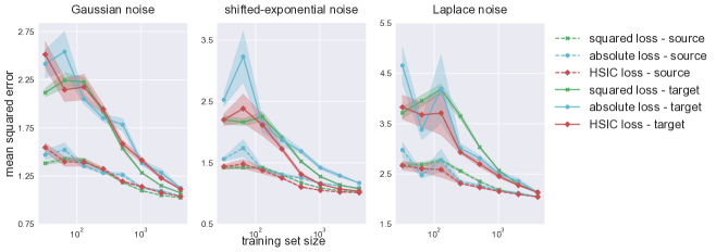
Figure 1: Comparison of models trained with squared-loss, absolute-loss and HSIC-loss. Each point on the graph is the MSE averaged over 20 experiments, and the shaded area represents one standard error from the mean. Dashed lines are the MSE evaluated over the source distribution, solid lines are the MSE evaluated over the target distribution.

As a first evaluation of the HSIC-loss, we experiment with fitting a linear model. We focus on small sample sizes as those often lead to difficulties in covariate shift scenarios. The underlying model in the experiments is $y=\beta^{\top}x+\varepsilon$ where $\beta\in\mathbb{R}^{100}$ is drawn for each experiment from a Gaussian distribution with $\sigma=0.1$. In the training phase, $x$ is drawn from a uniform distribution over $[-1,1]^{100}$. We experimented with $\varepsilon$ drawn from one of three distributions: Gaussian, Laplacian, or a shifted exponential: $\varepsilon=1-e$ where $e$ is drawn from an exponential distribution $\exp(1)$. In any case, $\varepsilon$ is drawn independently from $x$. In each experiment, we draw $n\in\{2^{i}\}_{i=5}^{13}$ training samples and train using either using squared-loss, absolute-loss, and HSIC-loss, all with an $l_{2}$ regularization term. The source test set is created in the same manner as the training set was created, while the target test set simulates a covariate shift scenario. This is done by changing the marginal distribution of $x$ from a uniform distribution to a Gaussian distribution over $\mathbb{R}^{100}$. In all cases the noise on the source and target is drawn from the same distribution. This process is repeated $20$ times for each $n$. When training the models with HSIC-loss, we used batch-size of 32, and optimized using Adam optimizer (Kingma and Ba, 2014). The kernels we chose were radial basis function kernels, with $\gamma=1$ for both covariates’ and residuals’ kernels.

Figure 1 presents the results of experiments with Gaussian, Laplacian, and shifted-exponential noise. With Gaussian noise, HSIC-loss performs similarly to squared-loss regression, and with Laplacian noise HSIC-loss performs similarly to absolute-loss regression, where squared-loss is the maximum-likelihood objective for Gaussian noise and absolute-loss is the maximum-likelihood objective for Laplacian noise. In both cases it is reassuring to see that HSIC-loss is on par with the maximum-likelihood objectives. In all cases we see that HSIC-loss is better on the target distribution compared to objectives which are not the maximum likelihood objective. This is true especially in small sample sizes. We believe this reinforces our result in Theorem 6 that the HSIC-loss is useful when we do not know in advance the loss or the exact target distribution.

6.2 Bike Sharing Dataset

In the bike sharing dataset by Fanaee-T and Gama (2014) from the UCI repository, the task is to predict the number of hourly bike rentals based on the following covariates: temperature, feeling temperature, wind speed and humidity. Consisting of 17,379 samples, the data was collected over two years, and can be partitioned by year and season. This dataset has been used to examine domain adaptation tasks by Subbaswamy et al. (2019) and Rothenhäusler et al. (2018). We adopt their setup, where the source distribution used for training is three seasons of a year, and the target distribution used for testing is the forth season of the same year, and where the model of choice is linear. We compare with least squares, anchor regression (AR) Rothenhäusler et al. (2018) and Surgery by Subbaswamy et al. (2019).

We ran 100 experiments, each of them was done by randomly sub-sampling $80\%$ of the source set and $80\%$ of the target set, thus obtaining a standard error estimate of the mean. When training the models with HSIC-loss, we used batch-size of 32, and optimized the loss with Adam (Kingma and Ba, 2014), with learning rate drawn from a uniform distribution over $[0.0008,0.001]$. The kernels we chose were radial basis function kernels, with $\gamma=2$ for the covariates’ kernel, and $\gamma=1$ for the residuals’ kernel.

We present the results in Table 1. Following the discussion in section 4, we report the variance of the residuals in the test set. We can see that training with HSIC-loss results in better performances in 6 out of 8 times. In addition, unlike AR and Surgery, training with HSIC-loss does not require knowledge of the specific causal graph of the problem, nor does it require the training to be gathered from different sources as in AR.

Table 1: Variance results on the bike sharing dataset. Each row corresponds to a training set consisting of three season of that year, and the variance of $Y-h(X)$ on the target set consisting of the forth season is reported. In bold are the best results in each experiment, taking into account one standard error.

Test data	OLS	AR	Surgery	HSIC
(Y1) Season 1	15.4$\pm$0.02	15.4$\pm$0.02	15.5$\pm$0.03	16.0$\pm$0.04
Season 2	23.1$\pm$0.03	23.1$\pm$0.03	23.7$\pm$0.04	22.9$\pm$0.03
Season 3	28.0$\pm$0.03	28.0$\pm$0.03	28.1$\pm$0.03	27.9$\pm$0.03
Season 4	23.7$\pm$0.03	23.7$\pm$0.03	25.6$\pm$0.04	23.6$\pm$0.04
(Y2) Season 1	29.8$\pm$0.05	29.8$\pm$0.05	30.7$\pm$0.06	30.7$\pm$0.07
Season 2	39.0$\pm$0.05	39.1$\pm$0.05	39.2$\pm$0.06	38.9$\pm$0.04
Season 3	41.7$\pm$0.05	41.5$\pm$0.05	41.8$\pm$0.05	40.8$\pm$0.05
Season 4	38.7$\pm$0.04	38.6$\pm$0.04	40.3$\pm$0.06	38.6$\pm$0.05

6.3 Rotating MNIST

In this experiment we test the performance of models trained on the MNIST dataset by LeCun et al. (1998) as the source distribution, and digits which are rotated by an angle $\theta$ sampled from a uniform distribution over $[-45,45]$ as the target distribution. Samples of the test data are depicted in the supplementary material. The standard approach to obtain robustness against such perturbations is to augment the training data with images with similar transformations, as in Schölkopf et al. (1996) for example. However, in practice it is not always possible to know in advance what kind of perturbations should be expected, and therefore it is valuable to develop methods for learning robust models even without such augmentations. We compared training with HSIC-loss to training with cross entropy loss, using three types of architectures. The first is a convolutional neural network (CNN):$\to$ input $\to$ conv(dim=32)$\to$ conv(dim=64) $\to$ fully-connected(dim=524)$\to$ dropout(p=0.5) $\to$ fully-connected(dim=10). The second is a multi-layered perceptron (MLP) with two hidden layers of size $256,524,1024$: input $\to$ fully-connected(dim=256,524,1024) $\to$ fully-connected(dim=256,524,1024)$\to$dropout(p=0.5) $\to$ fully-connected(dim=10). The third architecture was also an MLP, except there were four hidden layers instead of two. Each experiment was repeated 20 times, and in every experiment the number of training steps (7 epochs) remained constant for a fair comparison. Each time the training set consisted of 10K randomly chosen samples. The kernels we chose were radial basis function kernels with $\gamma=1$ for the residuals, and $\gamma=22$ for the images, chosen according to the heuristics suggested by Mooij et al. (2009). The results are depicted in Figure 2. We see that for all models, moving to the target distribution induces a large drop in accuracy. Yet for all architectures we see that using HSIC-loss gives better performance on the target set compared to using the standard cross-entropy loss.

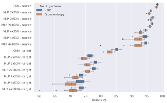
Figure 2: Accuracy on source and target test sets, with models trained with either cross entropy or HSIC-loss. Plotted are the median, 25th and 75th percentiles.

6.4 Cell Out of Sample Dataset

In the last experiment, we test our approach on the cell out of sample dataset introduced by Lu et al. (2019). This dataset was collected for the purpose of measuring robustness against covariate shift. It consists of $64\times 64$ microscopy images of mouse cells stained with one of seven possible fluorescent proteins (highlighting distinct parts of the cell), and the task is to predict the type of the fluorescent protein used to stain the cell. Learning systems trained on microscopy data are known to suffer from changes in plates, wells and instruments (Caicedo et al., 2017). Attempting to simulate these conditions, the dataset contains four test sets, with increasing degrees of change in the covariates’ distribution, as described in Table 2, adopted from Lu et al. (2019). Following (Lu et al., 2019), we trained an 11-layer CNN, DeepLoc, used in (Kraus et al., 2017) for protein subcellular localization. We followed the pre-processing, data augmentation, architecture choice, and training procedures described there, with the exception of using HSIC-loss and different learning rate when using HSIC. When computing HSIC, the kernel width was set to 1 for both kernels. Training was done for 50 epochs on 80% of the source dataset, and the final model was chosen according to the remaining 20% used as a validation set. The optimization was done with Adam (Kingma and Ba, 2014), with batch size of 128, and exponential decay of the learning rate was used when training with cross-entropy loss. Lu et al. (2019) used data augmentation during training (random cropping and random flips) and test time (prediction is averaged over 5 crops taken from the corners and center image), as this is a common procedure to encourage robustness. We compared HSIC-based models to cross-entropy based models both with and without test time augmentation. We note that (Lu et al., 2019) examined several deep net models and DeepLoc (with cross-entropy training) had the best results.

Table 2: Description of the source and target distributions in the cell out of sample dataset

Dataset	Description	Size
Source	Images from 4 independent plates for each class	41,456
Target1	Held out data	10,364
Target2	Same plates, but different wells	17,021
Target3	2 independent plates for each class, different days	32,596
Target4	1 plate for each class, different day and microscope	30,772

Table 3: Class balanced accuracy on each of the four target distributions. The last row depicts the results of training with cross-entropy as reported in (Lu et al., 2019). HSIC-aug and CE-aug refer to experiments done with test time augmentation.

Training loss	Target1	Target2	Target3	Target4
HSIC	99.2	98.8	93.4	95.3
CE	98.4	98.1	91.7	93.8
HSIC-aug	99.2	98.9	93.4	95.4
CE-aug-(Lu et al., 2019)	98.8	98.5	92.6	94.6

Table 3 depicts the results, showing a clear advantage of the HSIC-based model which is able to achieve new state-of-the-art results in the more difficult target distributions, while preserving the performance in target distributions closer to the source.

7 Conclusion

In this paper we propose learning models whose errors are independent of their inputs. This can be viewed as a non-parametric generalization of the way residuals are orthogonal to the instances in OLS regression. We prove that the HSIC-loss is learnable in terms of uniform convergence, and show that this loss naturally comes with a strong notion of robustness against changes in the input distribution when the change can be described in a bounded RKHS. The main theoretical limitations of our approach are the assumption that the changes are only in the marginal distribution of $X$, and that those changes are smooth in some sense. However, we show in our experiments that, in comparison to standard loss functions, the HSIC-loss produces models which perform just as well on the source distribution, and are significantly better on the target distribution, including state-of-the-art results on a challenging benchmark. An interesting future direction is to better understand the connection between this type of loss, originally proposed in the context of learning causal graph structure, and the idea of learning causal models that are expected to be robust against distributional changes (Meinshausen, 2018; Arjovsky et al., 2019).

8 Acknowledgments

The authors would like to thank David Lopez-Paz for helpful discussions. This research was partially supported by the Israel Science Foundation (grant No. 1950/19).

9 Appendix

9.1 Batch-size effect

Here we experiment with the effect of the batch-size on the performance of the HSIC-loss. The empirical HSIC value estimated on $m$ samples has bias of $O(1/m)$. This suggests that training with small batch-size might have a strong negative effect. However, in practice we have found that beyond the obvious computational cost of large batches (which scales as $m^{2}$), using larger mini-batches lead to worse performance in terms of accuracy. In the attached PDF we show that performance on the synthetic data setup using $m=64$ or 128 is considerably worse than $m=32$. We leave investigating the reasons for this interesting behavior, and the dynamics of gradients of HSIC in general, to future work.

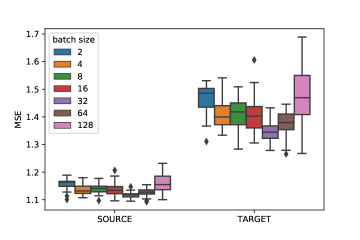
Figure 3: Effect of batch-size on performance on the linear regression experiment.

9.2 Theorems’ implications

In unsupervised covariate shift scenarios, there is always a tradeoff between how different do we allow the target distribution to be, versus the guarantees we can give for the target performance of a model trained on the source. In this work, we focus on specifying this tradeoff in terms of norms of RKHS spaces: the norm controls the complexity of the allowable target distribution set, and also multiplies components of the bounds. In the discussion of the theorems we argued that for $f^{\star}$ and functions near it, our bounds are much tighter compared to a bounds based on the infinity norm of the density ratio. Indeed, note that plugging $h=f^{\star}$ in Theorem 6 we get:

$$\sup_{\begin{subarray}{c}P_{\text{target}}\in\mathcal{Q}\\ \ell\in\mathcal{G}\end{subarray}}\mathbb{E}_{x\sim P_{\text{target}}}[\ell(Y-f^{\star}(X))]-\mathbb{E}_{x\sim P_{\text{source}}}[\ell(Y-f^{\star}(X))]$$

$$\leq 0,$$

which is a tight bound. When attempting to give a similar result using the infinity-norm of $\frac{P_{\text{target}}}{P_{\text{source}}}-1$, the bounds become far from tight:

$$\sup_{\begin{subarray}{c}P_{\text{target}}\in\mathcal{Q}\\ \ell\in\mathcal{G}\end{subarray}}\mathbb{E}_{x\sim P_{\text{target}}}[\ell(Y-f^{\star}(X))]-\mathbb{E}_{x\sim P_{\text{source}}}[\ell(Y-f^{\star}(X))]$$

$$=\sup_{\begin{subarray}{c}P_{\text{target}}\in\mathcal{Q}\\ \ell\in\mathcal{G}\end{subarray}}\mathbb{E}_{x\sim P_{\text{source}}}\left[\left(\frac{P_{\text{target}}}{P_{\text{source}}}-1\right)\ell(Y-f^{\star}(X))\right]$$

$$\leq C\cdot\sup_{\begin{subarray}{c}P_{\text{target}}\in\mathcal{Q}\\ \ell\in\mathcal{G}\end{subarray}}\mathbb{E}_{x\sim P_{\text{source}}}[\ell(Y-f^{\star}(X))],$$

where $C$ bounds the infinity norm of $\frac{P_{\text{target}}}{P_{\text{source}}}-1$. The fact that the HSIC bound is tighter justifies its use a loss function better suited for dealing with unsupervised covariate shift compared to simply minimizing a standard loss such as MSE. This tighter bound comes at a cost: there are many cases where the infinity-norm of $\frac{P_{\text{target}}}{P_{\text{source}}}-1$ is bounded but the Hilbert norm is unbounded, meaning that the density-ratio is not within the RKHS. Consider $p(k)=a/k^{2},q(k)=b/(k+1)^{2}$ for $k=1,2,...$ , where $a$ and $b$ are the normalizing constants and $k$ is all positive integers. In this case $||q/p-1||_{\infty}$ is bounded by roughly $1.55$, but the $l_{2}$ norm diverges to infinity. This means that our set of distributions $\mathcal{Q}$ is a strictly smaller subset of the set of infinity-norm bounded ratios, while our bounds are correspondingly more informative.

9.3 Proofs

Bellow we give the omitted proofs.

9.3.1 Optimality proof

We prove that $Y-h(X)\mathbin{\mathchoice{\hbox to0.0pt{\hbox{\set@color$\displaystyle\perp$}\hss}\kern 3.46875pt{}\kern 3.46875pt\hbox{\set@color$\displaystyle\perp$}}{\hbox to0.0pt{\hbox{\set@color$\textstyle\perp$}\hss}\kern 3.46875pt{}\kern 3.46875pt\hbox{\set@color$\textstyle\perp$}}{\hbox to0.0pt{\hbox{\set@color$\scriptstyle\perp$}\hss}\kern 2.36812pt{}\kern 2.36812pt\hbox{\set@color$\scriptstyle\perp$}}{\hbox to0.0pt{\hbox{\set@color$\scriptscriptstyle\perp$}\hss}\kern 1.63437pt{}\kern 1.63437pt\hbox{\set@color$\scriptscriptstyle\perp$}}}X$ implies that $Y\mathbin{\mathchoice{\hbox to0.0pt{\hbox{\set@color$\displaystyle\perp$}\hss}\kern 3.46875pt{}\kern 3.46875pt\hbox{\set@color$\displaystyle\perp$}}{\hbox to0.0pt{\hbox{\set@color$\textstyle\perp$}\hss}\kern 3.46875pt{}\kern 3.46875pt\hbox{\set@color$\textstyle\perp$}}{\hbox to0.0pt{\hbox{\set@color$\scriptstyle\perp$}\hss}\kern 2.36812pt{}\kern 2.36812pt\hbox{\set@color$\scriptstyle\perp$}}{\hbox to0.0pt{\hbox{\set@color$\scriptscriptstyle\perp$}\hss}\kern 1.63437pt{}\kern 1.63437pt\hbox{\set@color$\scriptscriptstyle\perp$}}}X\mid h(X)$.

Proof.

First, we note that this is equivalent to prove that $Y-h(X)\mathbin{\mathchoice{\hbox to0.0pt{\hbox{\set@color$\displaystyle\perp$}\hss}\kern 3.46875pt{}\kern 3.46875pt\hbox{\set@color$\displaystyle\perp$}}{\hbox to0.0pt{\hbox{\set@color$\textstyle\perp$}\hss}\kern 3.46875pt{}\kern 3.46875pt\hbox{\set@color$\textstyle\perp$}}{\hbox to0.0pt{\hbox{\set@color$\scriptstyle\perp$}\hss}\kern 2.36812pt{}\kern 2.36812pt\hbox{\set@color$\scriptstyle\perp$}}{\hbox to0.0pt{\hbox{\set@color$\scriptscriptstyle\perp$}\hss}\kern 1.63437pt{}\kern 1.63437pt\hbox{\set@color$\scriptscriptstyle\perp$}}}X\mid h(X)$, since the conditioning makes $h(X)$ just a constant. Now,

$$\begin{split}&P\left(Y-h(X)\mid X,h(X)\right)\\ &=P\left(Y-h(X)\mid X\right)\\ &=P\left(Y-h(X)\right)\\ &=P\left(Y-h(X)\mid h(X)\right),\end{split}$$

where the last equality is due to the fact that if the residual is independent of $X$, it is also independent of $h(X)$ ∎

9.3.2 Proof of lemma 2

Proof.

We prove that $\sup_{s\in\mathcal{F},t\in\mathcal{G}}\mathbb{C}\text{ov}[s(X),t(Y)]\leq M_{\mathcal{F}}\cdot M_{\mathcal{G}}\sup_{s\in\tilde{\mathcal{F}},t\in\tilde{\mathcal{G}}}\mathbb{C}\text{ov}[s(X),t(Y)]$. The other direction of the inequality is true by that same arguments.

Let $\{s_{i}\}_{i=1}^{\infty}\subset\mathcal{F}$ and $\{t_{i}\}_{i=1}^{\infty}\subset\mathcal{G}$ be such that

$$\lim_{n\to\infty}\mathbb{C}\text{ov}[s_{i}(X),t_{i}(Y)]=\sup_{s\in\mathcal{F},t\in\mathcal{G}}\mathbb{C}\text{ov}[s(X),t(Y)].$$

Since for all $i$, $\frac{1}{M_{\mathcal{F}}}\cdot s_{i}\in\tilde{\mathcal{F}}$ and likewise $\frac{1}{M_{\mathcal{G}}}\cdot t_{i}\in\tilde{\mathcal{G}}$, we have that

$$\sup_{s\in\mathcal{F},t\in\mathcal{G}}\mathbb{C}\text{ov}[s(X),t(Y)]$$

$$=\lim_{n\to\infty}\mathbb{C}\text{ov}[s_{i}(X),t_{i}(Y)]$$

$$=M_{\mathcal{F}}\cdot M_{\mathcal{G}}\lim_{n\to\infty}\mathbb{C}\text{ov}[\frac{1}{M_{\mathcal{F}}}s_{i}(X),\frac{1}{M_{\mathcal{G}}}t_{i}(Y)]$$

$$\leq M_{\mathcal{F}}\cdot M_{\mathcal{G}}\sup_{s\in\tilde{\mathcal{F}},t\in\tilde{\mathcal{G}}}\mathbb{C}\text{ov}[s(X),t(Y)].$$

∎

9.3.3 Proof of theorem 3

Proof.

Expanding the HSIC-loss:

$$\text{HSIC}(X,Y-h(X);\tilde{\mathcal{F}},\tilde{\mathcal{G}})$$

$$\geq \sup_{s\in\tilde{\mathcal{F}},t\in\tilde{\mathcal{G}}}\mathbb{C}\text{ov}\left(s\left(X\right),t\left(Y-h\left(X\right)\right)\right)$$

$$= \frac{1}{M_{\mathcal{F}}\cdot M_{\mathcal{G}}}\sup_{s\in\mathcal{F},t\in\mathcal{G}}\mathbb{C}\text{ov}\left(s\left(X\right),t\left(Y-h\left(X\right)\right)\right)$$

$$= \frac{1}{M_{\mathcal{F}}\cdot M_{\mathcal{G}}}\sup_{s\in\mathcal{F},t\in\mathcal{G}}\mathbb{C}\text{ov}\left(s\left(X\right),t\left(f^{\star}\left(X\right)-h\left(X\right)+\varepsilon\right)\right),$$

where the first inequality is due to Eq. (2), and the first equality by Lemma 2. Now, by the assumption that $f^{\star}-h$ is in the closure of $\mathcal{F}$, there exist $s_{n}\in\mathcal{F}$ s.t. $\left(s_{n}\right)_{n=1}^{\infty}$ converge to $f^{\star}-h$ under the infinity norm. Taking $t$ to be the identity function, we get that for all $n\in\mathbb{N}$:

$$\sup_{s\in\mathcal{F}}\mathbb{C}\text{ov}\left(s\left(X\right),f^{\star}\left(X\right)-h\left(X\right)+\varepsilon\right)$$

$$\geq\mathbb{C}\text{ov}\left(s_{n}\left(X\right),t\left(f^{\star}\left(X\right)-h\left(X\right)+\varepsilon\right)\right),$$

which implies that

$$\sup_{s\in\mathcal{F},t\in\mathcal{G}}\mathbb{C}\text{ov}\left(s\left(X\right),t\left(f^{\star}\left(X\right)-h\left(X\right)+\varepsilon\right)\right)$$

$$\geq \lim_{n\to\infty}\mathbb{C}\text{ov}\left(s_{n}\left(X\right),f^{\star}\left(X\right)-h\left(X\right)+\varepsilon\right)$$

$$= \mathbb{C}\text{ov}\left(f^{\star}\left(X\right)-h\left(X\right),f^{\star}\left(X\right)-h\left(X\right)+\varepsilon\right)$$

$$= \mathbb{V}\text{ar}\left(f^{\star}\left(X\right)-h\left(X\right)\right).$$

∎

9.3.4 Proof of theorem 5

Proof.

First, we note that

$$\begin{split}&\left|\mathbb{E}\left[s_{A}\left(x\right)\ell\left(y-h(x)\right)\right]-\mathbb{E}\left[1_{A}\left(x\right)\ell\left(y-h(x)\right)\right]\right|\\ &\leq\left|\mathbb{E}\left[\left(s_{A}\left(x\right)-1_{A}\left(x\right)\right)\ell\left(y-h(x)\right)\right]\right|\\ &\leq\mathbb{E}\left[\left|s_{A}\left(x\right)-1_{A}\left(x\right)\right|\ell\left(y-h(x)\right)\right]\\ &\leq\delta\mathbb{E}\left[\ell\left(y-h(x)\right)\right].\end{split}$$

And therefore

$$\begin{split}&\mathbb{E}\left[1_{A}\left(x\right)\ell\left(y-h(x)\right)\right]\\ &\leq\mathbb{E}\left[s_{A}\left(x\right)\ell\left(y-h(x)\right)\right]+\delta\mathbb{E}\left[\ell\left(y-h(x)\right)\right].\end{split}$$

Now, by definition,

$$\begin{split}&\mathbb{E}\left[s_{A}\left(x\right)\ell\left(y-h(x)\right)\right]\\ &\leq\mathbb{E}\left[s_{A}\left(x\right)\right]\mathbb{E}\left[\ell\left(y-h(x)\right)\right]\\ &+M_{\mathcal{F}}M_{\mathcal{G}}HSIC\left(x,y-h(x);\tilde{\mathcal{F}},\tilde{\mathcal{G}}\right).\end{split}$$

Similar to before,

$$\begin{split}&\left|\mathbb{E}\left[s_{A}\left(x\right)\right]\mathbb{E}\left[\ell\left(y-h(x)\right)\right]-\mathbb{E}\left[1_{A}\left(x\right)\right]\mathbb{E}\left[\ell\left(y-h(x)\right)\right]\right|\\ &\leq\delta\mathbb{E}\left[\ell\left(y-h(x)\right)\right],\end{split}$$

and therefore,

$$\begin{split}&\mathbb{E}\left[s_{A}\left(x\right)\right]\mathbb{E}\left[\ell\left(y-h(x)\right)\right]\\ &\leq\mathbb{E}\left[1_{A}\left(x\right)\right]\mathbb{E}\left[\ell\left(y-h(x)\right)\right]+\delta\mathbb{E}\left[\ell\left(y-h(x)\right)\right].\end{split}$$

Combining all the above:

$$\begin{split}&\frac{\mathbb{E}\left[1_{A}\left(x\right)\ell\left(y-h(x)\right)\right]}{\mathbb{E}\left[1_{A}\right]}\\ &\leq\frac{\mathbb{E}\left[s_{A}\left(x\right)\ell\left(y-h(x)\right)\right]+\delta\mathbb{E}\left[\ell\left(y-h(x)\right)\right]}{\mathbb{E}\left[1_{A}\right]}\\ &\leq\frac{\mathbb{E}\left[s_{A}\left(x\right)\right]\mathbb{E}\left[\ell\left(y-h(x)\right)\right]}{\mathbb{E}\left[1_{A}\right]}\\ &+\frac{M_{\mathcal{F}}M_{\mathcal{G}}HSIC\left(x,y-h(x);\tilde{\mathcal{F}},\tilde{\mathcal{G}}\right)+\delta\mathbb{E}\left[\ell\left(y-h(x)\right)\right]}{\mathbb{E}\left[1_{A}\right]}\\ &\leq\frac{\mathbb{E}\left[1_{A}\left(x\right)\right]\mathbb{E}\left[\ell\left(y-h(x)\right)\right]+\delta\mathbb{E}\left[\ell\left(y-h(x)\right)\right]}{\mathbb{E}\left[1_{A}\right]}\\ &+\frac{M_{\mathcal{F}}M_{\mathcal{G}}HSIC\left(x,y-h(x);\tilde{\mathcal{F}},\tilde{\mathcal{G}}\right)+\delta\mathbb{E}\left[\ell\left(y-h(x)\right)\right]}{\mathbb{E}\left[1_{A}\right]}\\ &=\frac{M_{\mathcal{F}}M_{\mathcal{G}}HSIC\left(x,y-h(x);\tilde{\mathcal{F}},\tilde{\mathcal{G}}\right)+2\delta\mathbb{E}\left[\ell\left(y-h(x)\right)\right]}{\mathbb{E}\left[1_{A}\right]}\\ &+\mathbb{E}\left[\ell\left(y-h(x)\right)\right]\\ &\leq\frac{M_{\mathcal{F}}M_{\mathcal{G}}HSIC\left(x,y-h(x);\tilde{\mathcal{F}},\tilde{\mathcal{G}}\right)+2\delta\mathbb{E}\left[\ell\left(y-h(x)\right)\right]}{c}\\ &+\mathbb{E}\left[\ell\left(y-h(x)\right)\right]\\ &=\frac{M_{\mathcal{F}}M_{\mathcal{G}}HSIC\left(x,y-h(x);\tilde{\mathcal{F}},\tilde{\mathcal{G}}\right)}{c}\\ &+\left(\frac{2\delta}{c}+1\right)\mathbb{E}\left[\ell\left(y-h(x)\right)\right]\end{split}$$

∎

9.3.5 Proof of theorem 6

Proof.

We have:

$$\begin{split}&\text{HSIC}(X,Y-h(X);\tilde{\mathcal{F}},\tilde{\mathcal{G}})\\ \geq&\sup_{s\in\tilde{\mathcal{F}},\ell\in\tilde{\mathcal{G}}}\bigg{(}\mathbb{E}_{x\sim\mathcal{P}}[s(X)\ell(Y-h(X))]\\ &-E_{x\sim\mathcal{P}_{\text{source}}}[s(X)]E_{x\sim\mathcal{P}_{\text{source}}}[\ell(Y-h(X))]\bigg{)}\\ =&\frac{1}{M_{\mathcal{F}}\cdot M_{\mathcal{G}}}\sup_{s\in\mathcal{F},\ell\in\mathcal{G}}\bigg{(}\mathbb{E}_{x\sim\mathcal{P}_{\text{source}}}[s(X)\ell(Y-h(X))]\\ &-\mathbb{E}_{x\sim\mathcal{P}_{\text{source}}}[s(X)]\mathbb{E}_{x\sim\mathcal{P}_{\text{source}}}[\ell(Y-h(X))]\bigg{)}\\ \geq&\frac{1}{M_{\mathcal{F}}\cdot M_{\mathcal{G}}}\sup_{s\in\mathcal{S},\ell\in\mathcal{G}}\bigg{(}\mathbb{E}_{x\sim\mathcal{P}_{\text{source}}}[s(X)\ell(Y-h(X))]\\ &-\mathbb{E}_{x\sim\mathcal{P}_{\text{source}}}[s(X)]\mathbb{E}_{x\sim\mathcal{P}_{\text{source}}}[\ell(Y-h(X))]\bigg{)}\\ =&\frac{1}{M_{\mathcal{F}}\cdot M_{\mathcal{G}}}\sup_{\mathcal{P}_{\text{target}}\in\mathcal{Q}}\sup_{\ell\in\mathcal{G}}\bigg{(}\mathbb{E}_{x\sim\mathcal{P}_{\text{target}}}[\ell(Y-h(X))]\\ &-\mathbb{E}_{x\sim\mathcal{P}_{\text{source}}}[\ell(Y-h(X))]\bigg{)}.\end{split}$$

The first equality is an immediate result of (2) and the identity $\mathbb{C}\text{ov}(A,B)=\mathbb{E}[AB]-\mathbb{E}[A]\mathbb{E}[B]$. The second inequality is by the restriction from $\mathcal{F}$ to $\mathcal{S}$. The final equality is by the assumption that for all $\mathcal{P}_{\text{target}}\in\mathcal{Q}$, $\mathbb{E}_{x\sim\mathcal{P}}\left[\frac{P_{\text{target}}}{P_{\text{source}}}(x)\right]=1$, i.e. that $\mathcal{P}_{\text{target}}$ is absolutely continuous with respect to $\mathcal{P}_{\text{source}}$. ∎

9.3.6 Proof of theorem 7

Proof.

By the lower bound of Theorem 3, we get $\mathbb{V}\text{ar}(f^{\star}(X)-h(X))\leq M_{\mathcal{F}}\cdot M_{\mathcal{G}}\cdot\delta_{\text{HSIC}}$. By Theorem 6 and the assumption we get that:

$$M_{\mathcal{F}}\cdot M_{\mathcal{G}}\cdot\delta_{\text{HSIC}}(h)$$

$$\geq \sup_{\mathcal{P}_{\text{target}}\in\mathcal{Q}}\mathbb{E}_{x\sim\mathcal{P}_{\text{target}}}[(Y-h(X))^{2}]-\mathbb{E}_{x\sim\mathcal{P}_{\text{source}}}[(Y-h(X))^{2}]$$

$$= \sup_{\mathcal{P}_{\text{target}}\in\mathcal{Q}}\bigg{(}\mathbb{E}_{x\sim\mathcal{P}_{\text{target}}}[(Y-h(X))^{2}]$$

$$-\mathbb{E}_{x\sim\mathcal{P}_{\text{source}}}[(f^{\star}(X)+\varepsilon-h(X))^{2}]\bigg{)}$$

$$= \sup_{\mathcal{P}_{\text{target}}\in\mathcal{Q}}\bigg{(}\mathbb{E}_{x\sim\mathcal{P}_{\text{target}}}[(Y-h(X))^{2}]-\mathbb{V}\text{ar}[f^{\star}(X)-h(X)]$$

$$-(\mathbb{E}_{x\sim\mathcal{P}_{\text{source}}}[f^{\star}(X)-h(X)])^{2}-\mathbb{E}[\varepsilon^{2}]\bigg{)}$$

$$= \sup_{\mathcal{P}_{\text{target}}\in\mathcal{Q}}\bigg{(}\textit{MSE}_{P_{\text{target}}}(h)-\mathbb{V}\text{ar}[f^{\star}(X)-h(X)]$$

$$-{\textit{bias}_{\text{source}}(h)}^{2}-\sigma^{2}\bigg{)}.$$

Together, these inequalities give the result. ∎

9.3.7 Proof of theorem 8

Bellow we give the proof of Theorem 8, showing uniform convergence for the HSIC-loss. The basic idea is to reduce the problem to a standard learning problem of the form $\sup_{h\in\mathcal{H}}\left|z(h)-\frac{1}{n}\sum_{i=1}^{n}z_{i}(h)\right|$, where $z$ is some statistic, and $z_{i}(h)$ are i.i.d. samples. To do so, we follow Gretton et al. [2005a], decomposing the HSIC-loss to three terms, and after some algebraic manipulations, and under some assumptions about the form of the kernel, we show that there is one term which we need to bound:

$$\sup_{h\in\mathcal{H}}\left|\mathbb{E}_{r,r^{\prime}}\left[k\left(r,r^{\prime}\right)\right]-\frac{1}{\left(n\right)_{2}}\sum_{i_{2}^{n}}k\left(r_{i_{1}},r_{i_{2}}\right)\right|.$$

We then show how we can treat this as a learning problem over pairs of instances, where the objective is to predict the difference in $y$, allowing us to use standard tools and concentration bounds.

Recall that the empirical estimation problem we pose is

$$\min_{\theta}\widehat{\text{HSIC}}\{(x_{i},r^{\theta}_{i})\}_{i=1}^{n};\mathcal{F},\mathcal{G})=\min_{\theta}\frac{1}{(m-1)^{2}}\textbf{tr}R^{\theta}HKH,$$ (6)

where $R^{\theta}_{i,j}=k(r_{i}^{\theta},r_{j}^{\theta}),\,r_{l}^{\theta}=y_{l}-h_{\theta}(x_{l}),$ and $K_{i,j}=l(x_{i},x_{j})$ and by the cyclic property of the trace we switched the positions of $R^{\theta}$ and $K$.

Lemma 9.

Let $C_{1}=\sup_{x,x^{\prime}}l(x,x^{\prime})$, $C_{2}=\sup_{r,r^{\prime}}k(r,r^{\prime})$. Then the following holds:

$$\sup_{h\in\mathcal{H}}\left|\text{HSIC}(X,Y-h(X);\mathcal{F},\mathcal{G})-\widehat{\text{HSIC}}\left(\{(x_{i},r_{i})\}_{i=1}^{n};\mathcal{F},\mathcal{G}\right)\right|$$

$$\leq 3C_{1}\cdot\sup_{h\in\mathcal{H}}\left|\mathbb{E}_{r,r^{\prime}}[k(r,r^{\prime})]-\frac{1}{(n)_{2}}\sum_{i_{2}^{n}}k(r_{i_{1}},r_{i_{2}})\right|$$

$$+3C_{2}\cdot\left|\mathbb{E}_{x,x^{\prime}}[l(x,x^{\prime}]-\frac{1}{(n)_{2}}\sum_{i_{2}^{n}}l(x_{i_{1}},x_{i_{2}})\right|$$

Proof.

Following [Gretton et al., 2005a], HSIC can be decomposed into a three part sum:

$$\begin{split}&HSIC\left(X,Y-h\left(X\right);\mathcal{F},\mathcal{G}\right)\\ =&\mathbb{E}_{x,x^{\prime},r,r^{\prime}}\left[k\left(r,r^{\prime}\right)l\left(x,x^{\prime}\right)\right]\\ &-2\mathbb{E}_{x,r}\left[\mathbb{E}_{x^{\prime}}\left[l\left(x,x^{\prime}\right)\right]\mathbb{E}_{r^{\prime}}\left[k\left(r,r^{\prime}\right)\right]\right]\\ &+\mathbb{E}_{r,r^{\prime}}\left[k\left(r,r^{\prime}\right)\right]\mathbb{E}_{x,x^{\prime}}\left[l\left(x,x^{\prime}\right)\right].\end{split}$$

And likewise, the empirical HSIC can be decomposed as follows:

$$\begin{split}&\widehat{HSIC}\left(\left\{\left(x_{i},r_{i}\right)\right\}_{i=1}^{n};\mathcal{F},\mathcal{G}\right)\\ =&\frac{1}{\left(n\right)_{2}}\sum_{i_{2}^{n}}k\left(r_{i_{1}},r_{i_{2}}\right)l\left(x_{i_{1}},x_{i_{2}}\right)\\ &-\frac{2}{\left(n\right)_{3}}\sum_{i_{3}^{n}}k\left(r_{i_{1}},r_{i_{2}}\right)l\left(x_{i_{2}},x_{i_{3}}\right)\\ &+\frac{1}{\left(n\right)_{4}}\sum_{i_{4}^{n}}k\left(r_{i_{1}},r_{i_{2}}\right)l\left(x_{i_{3}},x_{i_{4}}\right)+O\left(\frac{1}{n}\right).\end{split}$$

where $\left(n\right)_{m}=\frac{n!}{\left(n-m\right)!}$ and $i_{r}^{n}$ is the set of all $r-$tuples drawn without replacement from $[n]$. From this we can see that it is enough to bound the following three terms:

$$\sup_{h\in\mathcal{H}} \left|\vphantom{\sum_{i_{2}^{n}}}\mathbb{E}_{x,x^{\prime},r,r^{\prime}}\left[k\left(r,r^{\prime}\right)l\left(x,x^{\prime}\right)\right]\right.$$ (7)

$$\left.-\frac{1}{\left(n\right)_{2}}\sum_{i_{2}^{n}}k\left(r_{i_{1}},r_{i_{2}}\right)l\left(x_{i_{1}},x_{i_{2}}\right)\right|,$$ (8)

$$\begin{split}\sup_{h\in\mathcal{H}}&\left|\vphantom{\sum_{i_{2}^{n}}}\mathbb{E}_{x,r}\left[\mathbb{E}_{x^{\prime}}\left[l\left(x,x^{\prime}\right)\right]\mathbb{E}_{r^{\prime}}\left[k\left(r,r^{\prime}\right)\right]\right]\right.\\ &\left.-\frac{1}{\left(n\right)_{3}}\sum_{i_{3}^{n}}k\left(r_{i_{1}},r_{i_{2}}\right)l\left(x_{i_{2}},x_{i_{3}}\right)\right|,\end{split}$$ (9)

$$\begin{split}\sup_{h\in\mathcal{H}}&\left|\vphantom{\sum_{i_{2}^{n}}}\mathbb{E}_{r,r^{\prime}}\left[k\left(r,r^{\prime}\right)\right]\mathbb{E}_{x,x^{\prime}}\left[l\left(x,x^{\prime}\right)\right]\right.\\ &\left.-\frac{1}{\left(n\right)_{4}}\sum_{i_{4}^{n}}k\left(r_{i_{1}},r_{i_{2}}\right)l\left(x_{i_{3}},x_{i_{4}}\right)\right|.\end{split}$$ (10)

Using simple algebra, one can obtain the following bound for (7):

$$\begin{split}&\sup_{h\in\mathcal{H}}\left|\mathbb{E}_{x,x^{\prime},r,r^{\prime}}\left[k\left(r,r^{\prime}\right)l\left(x,x^{\prime}\right)\right]-\frac{1}{\left(n\right)_{2}}\sum_{i_{2}^{n}}k\left(r_{i_{1}},r_{i_{2}}\right)l\left(x_{i_{1}},x_{i_{2}}\right)\right|\\ =&\sup_{h\in\mathcal{H}}\left|\mathbb{E}_{x,x^{\prime},r,r^{\prime}}\left[k\left(r,r^{\prime}\right)l\left(x,x^{\prime}\right)\right]-\frac{1}{\left(n\right)_{2}}\sum_{i_{2}^{n}}k\left(r_{i_{1}},r_{i_{2}}\right)l\left(x_{i_{1}},x_{i_{2}}\right)\right.\\ &\left.+\frac{1}{\left(n\right)_{2}}\sum_{i_{2}^{n}}k\left(r_{i_{1}},r_{i_{2}}\right)\mathbb{E}\left[l\left(x,x^{\prime}\right)\right]-\frac{1}{\left(n\right)_{2}}\sum_{i_{2}^{n}}k\left(r_{i_{1}},r_{i_{2}}\right)\mathbb{E}\left[l\left(x,x^{\prime}\right)\right]\right|\\ =&\sup_{h\in\mathcal{H}}\left|\mathbb{E}_{x,x^{\prime},r,r^{\prime}}\left[\left(k\left(r,r^{\prime}\right)-\frac{1}{\left(n\right)_{2}}\sum_{i_{2}^{n}}k\left(r_{i_{1}},r_{i_{2}}\right)\right)l\left(x,x^{\prime}\right)\right]\right.\\ &\left.+\frac{1}{\left(n\right)_{2}}\sum_{i_{2}^{n}}k\left(r_{i_{1}},r_{i_{2}}\right)\left(\mathbb{E}\left[l\left(x,x^{\prime}\right)\right]-l\left(x_{i_{1}},x_{i_{2}}\right)\right)\right|\\ \leq&\sup_{h\in\mathcal{H}}\left|\mathbb{E}_{x,x^{\prime},r,r^{\prime}}\left[\left(k\left(r,r^{\prime}\right)-\frac{1}{\left(n\right)_{2}}\sum_{i_{2}^{n}}k\left(r_{i_{1}},r_{i_{2}}\right)\right)l\left(x,x^{\prime}\right)\right]\right|\\ &+\sup_{h\in\mathcal{H}}\left|\frac{1}{\left(n\right)_{2}}\sum_{i_{2}^{n}}k\left(r_{i_{1}},r_{i_{2}}\right)\left(\mathbb{E}\left[l\left(x,x^{\prime}\right)\right]-l\left(x_{i_{1}},x_{i_{2}}\right)\right)\right|\\ \leq&C_{1}\sup_{h\in\mathcal{H}}\left|\mathbb{E}_{x,x^{\prime},r,r^{\prime}}\left[k\left(r,r^{\prime}\right)-\frac{1}{\left(n\right)_{2}}\sum_{i_{2}^{n}}k\left(r_{i_{1}},r_{i_{2}}\right)\right]\right|\\ &+C_{2}\sup_{h\in\mathcal{H}}\left|\mathbb{E}\left[l\left(x,x^{\prime}\right)\right]-\frac{1}{\left(n\right)_{2}}\sum_{i_{2}^{n}}l\left(x_{i_{1}},x_{i_{2}}\right)\right|\\ =&C_{1}\sup_{h\in\mathcal{H}}\left|\mathbb{E}_{r,r^{\prime}}\left[k\left(r,r^{\prime}\right)\right]-\frac{1}{\left(n\right)_{2}}\sum_{i_{2}^{n}}k\left(r_{i_{1}},r_{i_{2}}\right)\right|\\ &+C_{2}\left|\mathbb{E}\left[l\left(x,x^{\prime}\right)\right]-\frac{1}{\left(n\right)_{2}}\sum_{i_{2}^{n}}l\left(x_{i_{1}},x_{i_{2}}\right)\right|.\end{split}$$

Where the first inequality follows from properties of $\sup$, the second inequality follows from the definitions of $C_{1}$ and $C_{2}$, and the last equality follows from the fact that the second term does not depend on $h$. Similarly, (9) can be bounded as follows:

$$\begin{split}&\sup_{h\in\mathcal{H}}\left|\vphantom{\sum_{i_{2}^{n}}}\mathbb{E}_{x,r}\left[\mathbb{E}_{x^{\prime}}\left[l\left(x,x^{\prime}\right)\right]\mathbb{E}_{r^{\prime}}\left[k\left(r,r^{\prime}\right)\right]\right]\right.\\ &\left.-\frac{1}{\left(n\right)_{3}}\sum_{i_{3}^{n}}k\left(r_{i_{1}},r_{i_{2}}\right)l\left(x_{i_{2}},x_{i_{3}}\right)\right|\\ =&\sup_{h\in\mathcal{H}}\left|\vphantom{\sum_{i_{2}^{n}}}\mathbb{E}_{x,r}\left[\mathbb{E}_{x^{\prime}}\left[l\left(x,x^{\prime}\right)\right]\mathbb{E}_{r^{\prime}}\left[k\left(r,r^{\prime}\right)\right]\right]\right.\\ &\left.-\frac{1}{\left(n\right)_{3}}\sum_{i_{3}^{n}}k\left(r_{i_{1}},r_{i_{2}}\right)l\left(x_{i_{2}},x_{i_{3}}\right)\right.\\ &+\left.{}\frac{1}{\left(n\right)_{3}}\sum_{i_{3}^{n}}k\left(r_{i_{1}},r_{i_{2}}\right)\mathbb{E}_{x,x^{\prime}}\left[l\left(x,x^{\prime}\right)\right]\right.\\ &\left.-\frac{1}{\left(n\right)_{3}}\sum_{i_{3}^{n}}k\left(r_{i_{1}},r_{i_{2}}\right)\mathbb{E}_{x,x^{\prime}}\left[l\left(x,x^{\prime}\right)\right]\right|\\ =&\sup_{h\in\mathcal{H}}\left|\vphantom{\sum_{i_{2}^{n}}}\mathbb{E}_{x,r}\left[\vphantom{\sum_{i_{2}^{n}}}\mathbb{E}_{x^{\prime}}\left[l\left(x,x^{\prime}\right)\right]\mathbb{E}_{r^{\prime}}\left[k\left(r,r^{\prime}\right)\right]\right.\right.\\ &\left.\left.-\frac{1}{\left(n\right)_{3}}\sum_{i_{3}^{n}}k\left(r_{i_{1}},r_{i_{2}}\right)\mathbb{E}_{x^{\prime}}\left[l\left(x,x^{\prime}\right)\right]\right]\right.\\ &\left.+\frac{1}{\left(n\right)_{3}}\sum_{i_{3}^{n}}k\left(r_{i_{1}},r_{i_{2}}\right)\left(\mathbb{E}_{x,x^{\prime}}\left[l\left(x,x^{\prime}\right)\right]-l\left(x_{i_{2}},x_{i_{3}}\right)\right)\right|\\ =&\sup_{h\in\mathcal{H}}\left|\mathbb{E}_{x,r}\left[\frac{1}{\left(n\right)_{3}}\sum_{i_{3}^{n}}\bigg{(}\mathbb{E}_{r^{\prime}}\left[k\left(r,r^{\prime}\right)\right]\right.\right.\\ &\left.\left.-k\left(r_{i_{1}},r_{i_{2}}\right)\bigg{)}\mathbb{E}_{x^{\prime}}\left[l\left(x,x^{\prime}\right)\right]\vphantom{\sum_{i_{2}^{n}}}\right]\right.\\ &\left.+\frac{1}{\left(n\right)_{3}}\sum_{i_{3}^{n}}k\left(r_{i_{1}},r_{i_{2}}\right)\bigg{(}\mathbb{E}_{x,x^{\prime}}\left[l\left(x,x^{\prime}\right)\right]-l\left(x_{i_{2}},x_{i_{3}}\right)\bigg{)}\right|\\ \leq&\sup_{h\in\mathcal{H}}\left|\mathbb{E}_{x,r}\left[\frac{1}{\left(n\right)_{3}}\sum_{i_{3}^{n}}\bigg{(}\mathbb{E}_{r^{\prime}}\left[k\left(r,r^{\prime}\right)\right]\right.\right.\\ &\left.\left.\vphantom{\sum_{i_{2}^{n}}}-k\left(r_{i_{1}},r_{i_{2}}\right)\bigg{)}\mathbb{E}_{x^{\prime}}\left[l\left(x,x^{\prime}\right)\right]\right]\right|\\ &+\sup_{h\in\mathcal{H}}\left|\frac{1}{\left(n\right)_{3}}\sum_{i_{3}^{n}}k\left(r_{i_{1}},r_{i_{2}}\right)\bigg{(}\mathbb{E}_{x,x^{\prime}}\left[l\left(x,x^{\prime}\right)\right]-l\left(x_{i_{2}},x_{i_{3}}\right)\bigg{)}\right|\\ \leq&\sup_{x}\mathbb{E}_{x^{\prime}}\left[l\left(x,x^{\prime}\right)\right]\sup_{h\in\mathcal{H}}\left|\mathbb{E}_{x,r}\left[\mathbb{E}_{r^{\prime}}\left[k\left(r,r^{\prime}\right)\right]\vphantom{\sum_{i_{2}^{n}}}\right.\right.\\ &\left.\left.-\frac{1}{\left(n\right)_{3}}\sum_{i_{3}^{n}}k\left(r_{i_{1}},r_{i_{2}}\right)\right]\right|\\ &+\sup_{r,r^{\prime}}k\left(r,r^{\prime}\right)\sup_{h\in\mathcal{H}}\left|\mathbb{E}_{x,x^{\prime}}\left[l\left(x,x^{\prime}\right)\right]-\frac{1}{\left(n\right)_{3}}\sum_{i_{3}^{n}}l\left(x_{i_{2}},x_{i_{3}}\right)\right|\\ \leq&C_{1}\sup_{h\in\mathcal{H}}\left|\mathbb{E}_{r,r^{\prime}}\left[k\left(r,r^{\prime}\right)\right]-\frac{1}{\left(n\right)_{2}}\sum_{i_{2}^{n}}k\left(r_{i_{1}},r_{i_{2}}\right)\right|\\ &+C_{2}\left|\mathbb{E}_{x,x^{\prime}}\left[l\left(x,x^{\prime}\right)\right]-\frac{1}{\left(n\right)_{2}}\sum_{i_{2}^{n}}l\left(x_{i_{1}},x_{i_{2}}\right)\right|,\end{split}$$

where the first inequality follows from properties of $\sup$, and the last inequality follows from the definition of $C_{1}$ and $C_{2}$, and the definitions of $(n)_{m}$. And finally, the same reasoning can be applied to bound (10):

$$\begin{split}&\sup_{h\in\mathcal{H}}\left|\vphantom{\sum_{i_{2}^{n}}}\mathbb{E}_{r,r^{\prime}}\left[k\left(r,r^{\prime}\right)\right]\mathbb{E}_{x,x^{\prime}}\left[l\left(x,x^{\prime}\right)\right]\right.\\ &\left.-\frac{1}{\left(n\right)_{4}}\sum_{i_{4}^{n}}k\left(r_{i_{1}},r_{i_{2}}\right)l\left(x_{i_{3}},x_{i_{4}}\right)\right|\\ =&\sup_{h\in\mathcal{H}}\left|\mathbb{E}_{r,r^{\prime}}\left[k\left(r,r^{\prime}\right)\right]\mathbb{E}_{x,x^{\prime}}\left[l\left(x,x^{\prime}\right)\right]\right.\\ &\left.-\frac{1}{\left(n\right)_{4}}\sum_{i_{4}^{n}}k\left(r_{i_{1}},r_{i_{2}}\right)l\left(x_{i_{3}},x_{i_{4}}\right)\right.\\ &+\left.{}\frac{1}{\left(n\right)_{4}}\sum_{i_{4}^{n}}k\left(r_{i_{1}},r_{i_{2}}\right)\mathbb{E}_{x,x^{\prime}}\left[l\left(x,x^{\prime}\right)\right]\right.\\ &\left.-\frac{1}{\left(n\right)_{4}}\sum_{i_{4}^{n}}k\left(r_{i_{1}},r_{i_{2}}\right)\mathbb{E}_{x,x^{\prime}}\left[l\left(x,x^{\prime}\right)\right]\right|\\ =&\sup_{h\in\mathcal{H}}\left|\left(\mathbb{E}_{r,r^{\prime}}\left[k\left(r,r^{\prime}\right)\right]-\frac{1}{\left(n\right)_{4}}\sum_{i_{4}^{n}}k\left(r_{i_{1}},r_{i_{2}}\right)\right)\mathbb{E}_{x,x^{\prime}}\left[l\left(x,x^{\prime}\right)\right]\right.\\ &\left.+\frac{1}{\left(n\right)_{4}}\sum_{i_{4}^{n}}k\left(r_{i_{1}},r_{i_{2}}\right)\left(\mathbb{E}_{x,x^{\prime}}\left[l\left(x,x^{\prime}\right)\right]-l\left(x_{i_{3}},x_{i_{4}}\right)\right)\right|\\ \leq&\sup_{h\in\mathcal{H}}\left|\left(\mathbb{E}_{r,r^{\prime}}\left[k\left(r,r^{\prime}\right)\right]-\frac{1}{\left(n\right)_{4}}\sum_{i_{4}^{n}}k\left(r_{i_{1}},r_{i_{2}}\right)\right)\mathbb{E}_{x,x^{\prime}}\left[l\left(x,x^{\prime}\right)\right]\right|\\ &+\sup_{h\in\mathcal{H}}\left|\frac{1}{\left(n\right)_{4}}\sum_{i_{4}^{n}}k\left(r_{i_{1}},r_{i_{2}}\right)\left(\mathbb{E}_{x,x^{\prime}}\left[l\left(x,x^{\prime}\right)\right]-l\left(x_{i_{3}},x_{i_{4}}\right)\right)\right|\\ \leq&C_{1}\sup_{h\in\mathcal{H}}\left|\left(\mathbb{E}_{r,r^{\prime}}\left[k\left(r,r^{\prime}\right)\right]-\frac{1}{\left(n\right)_{2}}\sum_{i_{2}^{n}}k\left(r_{i_{1}},r_{i_{2}}\right)\right)\right|\\ &+C_{2}\left|\mathbb{E}_{x,x^{\prime}}\left[l\left(x,x^{\prime}\right)\right]-\frac{1}{\left(n\right)_{2}}\sum_{i_{2}^{n}}l\left(x_{i_{1}},x_{i_{2}}\right)\right|.\end{split}$$

∎

Now, the second term of the RHS of the bound in Lemma 9 can be bounded using standard techniques such as Hoeffding’s inequality. We therefore shift our attention to the first term. This term can be bounded using Rademacher based techniques.

Let us first recall the definition of the Rademacher complexity of a function class.

Definition 10.

Let $\mathcal{D}$ be a distribution over $Z$, and let $S=\{z_{i}\}_{i=1}^{n}$ be $n$ i.i.d. samples. The empirical Rademacher complexity of a function class $\mathcal{F}$ is defined as:

$$\mathcal{R}_{n}(\mathcal{F})=\mathbb{E}_{\sigma}\left[\sup_{f\in\mathcal{F}}\frac{1}{n}\sum_{i=1}^{n}\sigma_{i}h(z_{i})\right].$$

We assume that $k\left(r,r^{\prime}\right)=s\left(r-r^{\prime}\right)$ for some function $s$ with Lipschitz constant $L_{s}$. Next, we define a distribution over $\mathcal{X}\times\mathcal{X}\times\mathcal{Y}$ by $p^{\prime}\left(\boldsymbol{x}\right)=p^{\prime}\left(\left(x,x^{\prime}\right)\right)=p\left(x\right)p\left(x^{\prime}\right)$, and we let $y\left(x,x^{\prime},\varepsilon,\varepsilon^{\prime}\right)=f\left(x\right)-f\left(x^{\prime}\right)+\varepsilon-\varepsilon^{\prime}$. Now, we can define a new function class

$$\mathcal{H}^{2}=\left\{\left(x_{1},x_{2}\right)\mapsto h\left(x_{1}\right)-h\left(x_{2}\right)\mid h\in\mathcal{H}\right\},$$

and consider

$$\sup_{h\in\mathcal{H}^{2}}\left|\mathbb{E}_{\boldsymbol{x},y}\ell\left(h\left(\boldsymbol{x}\right),y\right)-\sum_{i=1}^{n}\ell(h(\textbf{x}_{i}),y_{i})\right|$$

where $\ell\left(h\left(\boldsymbol{x}\right),y\right)=s\left(r_{1}-r_{2}\right)$. This is exactly the first term in the bound, which can be bounded using standard generalization bounds. The only missing pieces left are how to relate the Rademacher complexity of $\mathcal{H}^{2}$ to that of $\mathcal{H}$, and how the Lipschitz constant of the residuals’ kernel affects it.

Lemma 11.

$\mathcal{R}_{n}(\mathcal{H}^{2})\leq 2\mathcal{R}_{n}(\mathcal{H})$.

Proof.

Let $S=\left\{(z_{i_{1}},z_{i_{2}})\right\}_{i}=1^{n}$. Then,

$$\mathcal{R}_{n}(\mathcal{H}^{2})= \mathbb{E}_{\sigma}\left[\sup_{h\in\mathcal{H}^{2}}\frac{1}{n}\sum_{i=1}^{n}\sigma_{i}h(s_{i})\right]$$

$$= \mathbb{E}_{\sigma}\left[\sup_{h\in\mathcal{H}}\frac{1}{n}\sum_{i=1}^{n}\sigma_{i}\left(h(z_{i_{1}})-h(z_{i_{2}})\right)\right]$$

$$\leq \mathbb{E}_{\sigma}\left[\sup_{h\in\mathcal{H}}\frac{1}{n}\sum_{i=1}^{n}\sigma_{i}h(z_{i_{1}})+\sup_{h\in\mathcal{H}}\frac{1}{n}\sum_{i=1}^{n}\sigma_{i}h(z_{i_{2}})\right]$$

$$= 2\mathcal{R}_{n}(\mathcal{H}),$$

where the inequality is due to algebra of $\sup$ and sums. ∎

As for the Lipschitz constant, a known result relating the Rademacher complexity of a function class to the Rademacher complexity of the class composed with a Lipschitz loss is the following.

Theorem 12 (Sham Kakade ).

Let $\ell:\,\mathbb{R}\times\mathcal{Y}\to\mathbb{R}$ be s.t. $\ell(\cdot,y)$ is an $L-$Lipschitz function for all $y$. Denote $\ell\circ\mathcal{H}=\left\{(x,y)\to\ell(h(x),y)\mid h\in\mathcal{H}\right\}$. Then,

$$\mathcal{R}_{n}(\ell\circ\mathcal{H})\leq L\cdot\mathcal{R}_{n}(\mathcal{H}).$$

As an example, the following lemma proves the Lipschitz condition for RBF kernels.

Lemma 13.

Assume $\ell(z,y)=\exp(-\gamma(z-y)^{2})$, as is the case with RBF kernels, and suppose $|y|\leq\frac{M}{2}$ for some $M>0$ for all $y$. Then $\ell(\cdot,y)$ is $\gamma M-$Lipschitz for all $y$.

Proof.

Let $\ell(z,y)=\exp\left(-\gamma\|z-y\|^{2}\right)$ for some $\gamma>0$, and suppose $\|y\|\leq\frac{M}{2}$ for some $M>0$ for all $y\in\mathcal{Y}$. Then,

$$\exp\left(-\gamma\|y-z_{1}\|^{2}\right)-\exp\left(-\gamma\|y-z_{2}\|^{2}\right)$$

$$= \exp\left(-\gamma\|y-z_{1}\|^{2}\right)\left(1-\exp\left(\gamma\left(\|y-z_{1}\|^{2}-\|y-z_{2}\|^{2}\right)\right)\right)$$

$$\leq \exp\left(-\gamma\|y-z_{1}\|^{2}\right)\left(1-\left(1+\gamma\left(\|y-z_{1}\|^{2}-\|y-z_{2}\|^{2}\right)\right)\right)$$

$$= \exp\left(-\gamma\|y-z_{1}\|^{2}\right)\left(\gamma\left(\|y-z_{2}\|^{2}-\|y-z_{1}\|^{2}\right)\right)$$

$$\leq \gamma\left(\|y-z_{2}\|^{2}-\|y-z_{1}\|^{2}\right)$$

$$\leq \gamma\|z_{1}-z_{2}\|^{2}$$

$$\leq \gamma\cdot M\|z_{1}-z_{2}\|$$

where the first inequality is due to the fact that $1+x\leq e^{x}$, the second is due to the fact that $\exp(-c)\leq 1\,\forall c\geq 0$, the third is due to triangle inequality and the last is due to the definition of $M$. ∎

Before concluding, we state the uniform convergence result based on the Rademacher complexity of a class.

Theorem 14 (Mohri et al. [2018], Ch. 3).

Suppose $f(z)\in[0,1]$ for all $f\in\mathcal{F}$, and let $\delta\in(0,1)$. Then, with probability of at least $1-\delta$ over the choice of $S$, the following holds uniformly for all $f\in\mathcal{F}$:

$$\left|\mathbb{E}_{\mathcal{P}}[f(z)]-\frac{1}{n}\sum_{i=1}^{n}f(z_{i})\right|\leq 2\mathcal{R}_{n}(\mathcal{F})+O\left(\sqrt{\frac{\ln(1/\delta)}{n}}\right).$$

Equipped with those results, the learnability Theorem 8 immediately follows.

Proof of Theorem 8.

This is a direct application of the previous lemmas and Hoeffding’s inequality. ∎

9.4 Experiments’ details

9.4.1 Synthetic data

In order to find the $l_{2}$ regularization parameter, we perform cross validation on validation data created from $10\%$ of the training set, where the possible values are in $\{15,12,10,5,1,0.1,0.01,0.001,0.0001,0.00001,0.000001,0\}$, for absolute- and HSIC-losses, and $\{35,37,...,69\}$ for the squared-loss.

When training with absolute-loss, we used stochastic gradient descent, with initial learning rate determined by cross validation from $\{0.05,0.01,0.005,0.001,0.0005,0.0001,0.00005,0.00001\}$, and later decayed using inverse scaling. When training with HSIC-loss, the learning rate was drawn from a uniform distribution over $[0.0001,0.0002]$.

9.4.2 Rotated MNIST

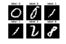
Figure 4: MNIST target images.

Both losses were optimized using Adam [Kingma2015AdamAM], and the learning rate was drawn each time from a uniform distribution over $[10^{-4},4\cdot 10^{-4}]$. Experimenting with different regimes of the learning rate gave similar results.

References

- Abadi et al. (2015) M. Abadi, A. Agarwal, P. Barham, E. Brevdo, Z. Chen, C. Citro, G. S. Corrado, A. Davis, J. Dean, M. Devin, S. Ghemawat, I. Goodfellow, A. Harp, G. Irving, M. Isard, Y. Jia, R. Jozefowicz, L. Kaiser, M. Kudlur, J. Levenberg, D. Mané, R. Monga, S. Moore, D. Murray, C. Olah, M. Schuster, J. Shlens, B. Steiner, I. Sutskever, K. Talwar, P. Tucker, V. Vanhoucke, V. Vasudevan, F. Viégas, O. Vinyals, P. Warden, M. Wattenberg, M. Wicke, Y. Yu, and X. Zheng. TensorFlow: Large-scale machine learning on heterogeneous systems, 2015. URL http://tensorflow.org/. Software available from tensorflow.org.
- Arjovsky et al. (2019) M. Arjovsky, L. Bottou, I. Gulrajani, and D. Lopez-Paz. Invariant risk minimization. arXiv preprint arXiv:1907.02893, 2019.
- Caicedo et al. (2017) J. C. Caicedo, S. Cooper, F. Heigwer, S. Warchal, P. Qiu, C. Molnar, A. S. Vasilevich, J. D. Barry, H. S. Bansal, O. Kraus, et al. Data-analysis strategies for image-based cell profiling. Nature methods, 14(9):849, 2017.
- Daume III and Marcu (2006) H. Daume III and D. Marcu. Domain adaptation for statistical classifiers. Journal of artificial Intelligence research, 26:101–126, 2006.
- Duchi and Namkoong (2018) J. Duchi and H. Namkoong. Learning models with uniform performance via distributionally robust optimization. arXiv preprint arXiv:1810.08750, 2018.
- Fanaee-T and Gama (2014) H. Fanaee-T and J. Gama. Event labeling combining ensemble detectors and background knowledge. Progress in Artificial Intelligence, 2(2-3):113–127, 2014.
- Gretton et al. (2005a) A. Gretton, O. Bousquet, A. Smola, and B. Schölkopf. Measuring statistical dependence with hilbert-schmidt norms. In International conference on algorithmic learning theory, pages 63–77. Springer, 2005a.
- Gretton et al. (2005b) A. Gretton, R. Herbrich, A. Smola, O. Bousquet, and B. Schölkopf. Kernel methods for measuring independence. Journal of Machine Learning Research, 6(Dec):2075–2129, 2005b.
- Gretton et al. (2008) A. Gretton, K. Fukumizu, C. H. Teo, L. Song, B. Schölkopf, and A. J. Smola. A kernel statistical test of independence. In Advances in neural information processing systems, pages 585–592, 2008.
- Gretton et al. (2009) A. Gretton, A. Smola, J. Huang, M. Schmittfull, K. Borgwardt, and B. Schölkopf. Covariate shift by kernel mean matching. Dataset shift in machine learning, 3(4):5, 2009.
- Heinze-Deml and Meinshausen (2017) C. Heinze-Deml and N. Meinshausen. Conditional variance penalties and domain shift robustness. arXiv preprint arXiv:1710.11469, 2017.
- Kingma and Ba (2014) D. P. Kingma and J. Ba. Adam: A method for stochastic optimization. arXiv preprint arXiv:1412.6980, 2014.
- Kraus et al. (2017) O. Z. Kraus, B. T. Grys, J. Ba, Y. Chong, B. J. Frey, C. Boone, and B. J. Andrews. Automated analysis of high-content microscopy data with deep learning. Molecular systems biology, 13(4), 2017.
- LeCun et al. (1998) Y. LeCun, L. Bottou, Y. Bengio, P. Haffner, et al. Gradient-based learning applied to document recognition. Proceedings of the IEEE, 86(11):2278–2324, 1998.
- Lu et al. (2019) A. Lu, A. Lu, W. Schormann, M. Ghassemi, D. Andrews, and A. Moses. The cells out of sample (coos) dataset and benchmarks for measuring out-of-sample generalization of image classifiers. In Advances in Neural Information Processing Systems, pages 1854–1862, 2019.
- Meinshausen (2018) N. Meinshausen. Causality from a distributional robustness point of view. In 2018 IEEE Data Science Workshop (DSW), pages 6–10. IEEE, 2018.
- Mohri et al. (2018) M. Mohri, A. Rostamizadeh, and A. Talwalkar. Foundations of machine learning. MIT press, 2018.
- Mooij et al. (2009) J. Mooij, D. Janzing, J. Peters, and B. Schölkopf. Regression by dependence minimization and its application to causal inference in additive noise models. In Proceedings of the 26th annual international conference on machine learning, pages 745–752. ACM, 2009.
- Namkoong and Duchi (2017) H. Namkoong and J. C. Duchi. Variance-based regularization with convex objectives. In Advances in Neural Information Processing Systems, pages 2971–2980, 2017.
- Paszke et al. (2019) A. Paszke, S. Gross, F. Massa, A. Lerer, J. Bradbury, G. Chanan, T. Killeen, Z. Lin, N. Gimelshein, L. Antiga, et al. Pytorch: An imperative style, high-performance deep learning library. In Advances in neural information processing systems, pages 8026–8037, 2019.
- Rényi (1959) A. Rényi. On measures of dependence. Acta mathematica hungarica, 10(3-4):441–451, 1959.
- Rosenfeld et al. (2018) A. Rosenfeld, R. Zemel, and J. K. Tsotsos. The elephant in the room. arXiv preprint arXiv:1808.03305, 2018.
- Rothenhäusler et al. (2018) D. Rothenhäusler, N. Meinshausen, P. Bühlmann, and J. Peters. Anchor regression: heterogeneous data meets causality. arXiv preprint arXiv:1801.06229, 2018.
- Saenko et al. (2010) K. Saenko, B. Kulis, M. Fritz, and T. Darrell. Adapting visual category models to new domains. In European conference on computer vision, pages 213–226. Springer, 2010.
- Schölkopf et al. (1996) B. Schölkopf, C. Burges, and V. Vapnik. Incorporating invariances in support vector learning machines. In Artificial Neural Networks: ICANN 96, LNCS vol. 1112, pages 47–52, Berlin, Germany, July 1996. Max-Planck-Gesellschaft, Springer. volume 1112 of Lecture Notes in Computer Science.
- (26) A. T. Sham Kakade. Rademacher composition and linear prediction. URL https://ttic.uchicago.edu/~tewari/lectures/lecture17.pdf.
- Subbaswamy and Saria (2018) A. Subbaswamy and S. Saria. Counterfactual normalization: Proactively addressing dataset shift using causal mechanisms. In 34th Conference on Uncertainty in Artificial Intelligence 2018, UAI 2018, pages 947–957. Association For Uncertainty in Artificial Intelligence (AUAI), 2018.
- Subbaswamy et al. (2019) A. Subbaswamy, P. Schulam, and S. Saria. Preventing failures due to dataset shift: Learning predictive models that transport. In The 22nd International Conference on Artificial Intelligence and Statistics, pages 3118–3127, 2019.
- Tzeng et al. (2017) E. Tzeng, J. Hoffman, K. Saenko, and T. Darrell. Adversarial discriminative domain adaptation. In Proceedings of the IEEE Conference on Computer Vision and Pattern Recognition, pages 7167–7176, 2017.
- Volpi et al. (2018a) R. Volpi, P. Morerio, S. Savarese, and V. Murino. Adversarial feature augmentation for unsupervised domain adaptation. In Proceedings of the IEEE Conference on Computer Vision and Pattern Recognition, pages 5495–5504, 2018a.
- Volpi et al. (2018b) R. Volpi, H. Namkoong, O. Sener, J. C. Duchi, V. Murino, and S. Savarese. Generalizing to unseen domains via adversarial data augmentation. In Advances in Neural Information Processing Systems, pages 5334–5344, 2018b.