Rapid escape of ultra-hot exoplanet atmospheres driven by hydrogen Balmer absorption

Abstract

Atmospheric escape is key to explaining the long-term evolution of planets in our Solar System and beyond, and in the interpretation of atmospheric measurements. Hydrodynamic escape is generally thought to be driven by the flux of extreme ultraviolet photons that the planet receives from its host star. Here, we show that the escape from planets orbiting hot stars proceeds through a different yet complementary process: drawing its energy from the intense near ultraviolet emission of the star that is deposited within an optically thin, high-altitude atmospheric layer of hydrogen excited into the lower state of the Balmer series. The ultra-hot exoplanet KELT-9b likely represents the first known instance of this Balmer-driven escape. In this regime of hydrodynamic escape, the near ultraviolet emission from the star is more important at determining the planet mass loss than the extreme ultraviolet emission, and uncertainties in the latter become less critical. Further, we predict that gas exoplanets around hot stars may experience catastrophic mass loss when they are less massive than 1–2 Jupiter masses and closer-in than KELT-9b, thereby challenging the paradigm that all large exoplanets are stable to atmospheric escape. We argue that extreme escape will affect the demographics of close-in exoplanets orbiting hot stars.

1 Introduction

Planet atmospheres subject to strong stellar irradiation undergo hydrodynamic escape that may affect the planets’ bulk properties if sustained over Gigayears, especially for the smaller, lower-mass planets (Lammer et al., 2008; Tian, 2015; Zahnle & Catling, 2017; Owen, 2019). This idea is supported by the statistics of the $>$4,000 exoplanets discovered to date, which show that specific combinations of planet size and stellar irradiation are underrepresented – a finding consistent with significant planet mass evolution (Lopez et al., 2012; Fulton et al., 2017; Jin & Mordasini, 2018). On the other hand, hydrodynamic escape is thought to affect minimally the evolution of Jupiter-mass and heavier planets. Also, in some instances atoms of suspected atmospheric origin have been detected at altitudes near or beyond the planets’ Roche lobe (Vidal-Madjar et al., 2003, 2004; Ben-Jaffel, 2007; Fossati et al., 2010; Lecavelier des Etangs et al., 2010; Linsky et al., 2010; Jensen et al., 2012; Kulow et al., 2014; Ballester & Ben-Jaffel, 2015; Ehrenreich et al., 2015; Bourrier et al., 2018; Salz et al., 2018; Spake et al., 2018; Sing et al., 2019), indicating that they are no longer gravitationally bound.

The generally accepted view of hydrodynamic escape in hydrogen-dominated atmospheres is that it is driven by stellar extreme ultraviolet (EUV; wavelengths $\lambda$$<$912 Å) photons deposited in the planet’s thermosphere (Lammer et al., 2003; Yelle, 2004; Tian et al., 2005; García Muñoz, 2007; Murray-Clay et al., 2009; Koskinen et al., 2013; Ionov et al., 2014; Guo & Ben-Jaffel, 2016; Salz et al., 2016). In that view, ground state hydrogen H(1) (principal quantum number $n$ in parentheses) plays the fundamental role of absorbing the incident photons in the Lyman continuum ($n$=1$\rightarrow$$\infty$) that ultimately heat the atmosphere. It is also tacitly assumed that no other gas competes with H(1) in terms of stellar energy absorption at these or other wavelengths in the thermosphere, even when absorption by metals at wavelengths longer than the Lyman continuum threshold is considered (García Muñoz, 2007; Koskinen et al., 2013). Our work challenges these ideas for, at least, the case of exoplanets orbiting hot stars.

The discovery of exoplanets around hot stars of effective temperatures $T_{\rm{eff}}$$>$7,500 K (Collier Cameron et al., 2010; Gaudi et al., 2017; Lund et al., 2017; Talens et al., 2018) and the detection of absorption by atomic gases in their atmospheres (Casasayas-Barris et al., 2018; Hoeijmakers et al., 2018; Yan & Henning, 2018; Cauley et al., 2019) has opened up new opportunities to test our understanding of hydrodynamic escape and in turn of exoplanet evolution. The hottest of these stars ($T_{\rm{eff}}$$>$8,200 K) present high levels of near-ultraviolet (NUV; for convenience loosely defined here as having $\lambda$$<$4,000 Å, although in strict terms that also includes the middle and far ultraviolet) emission but are not expected to be particularly strong EUV emitters (Fossati et al., 2018). The planets transiting two of such hot stars, KELT-9b and MASCARA-2b/KELT-20b, exhibit strong absorption in the H-$\alpha$ (6565 Å; $n$=2$\rightarrow$$n$=3) and -$\beta$ (4863 Å; $n$=2$\rightarrow$$n$=4) lines of the hydrogen Balmer series (Yan & Henning, 2018; Casasayas-Barris et al., 2018; Cauley et al., 2019). It is thus conceivable that Balmer continuum absorption ($n$=2$\rightarrow$$\infty$; $\lambda$$<$3646 Å), facilitated by large column abundances of thermospheric H(2), will tap into the enormous reservoir of energy in the stellar NUV emission. This represents a previously unconsidered source of energy to drive hydrodynamic escape that potentially outpaces the EUV-driven escape.

The condition for this to occur is $\tau_{\rm{BaC}}$$F^{\star}_{\rm{BaC}}$/$F^{\star}_{\rm{LyC}}$$\gtrsim$1, where $\tau_{\rm{BaC}}$ is the optical thickness at a representative Balmer continuum wavelength from the atmospheric top to the lower thermosphere, and $F^{\star}_{\rm{BaC}}$/$F^{\star}_{\rm{LyC}}$ is the ratio of wavelength-integrated stellar emission energies in the Balmer and Lyman continua. The condition derives from estimating the energy deposited at each wavelength range $\propto$$F^{\star}$$\left[1-\exp(-\tau)\right]$, and realizing that the thermosphere is optically thick at EUV wavelengths but thin in the NUV, i.e. $\tau_{\rm{LyC}}$$\gg$1 but $\tau_{\rm{BaC}}$$\ll$1. We estimate for the star KELT-9 (at 1 Astronomical Unit; see below), $F^{\star}_{\rm{LyC}}$=3.8 and $F^{\star}_{\rm{BaC}}$=2.9$\times$10⁷ erg s^-1 cm^-2, which results in the ratio $\sim$7.5$\times$10⁶. An optical thickness $\tau_{\rm{BaC}}$$\gtrsim$1.3$\times$10^-7 will turn the stellar NUV emission into the main source of energy deposited in KELT-9b’s thermosphere. For reference, typical values for the Sun ($T$_eff=5,800 K) are 4.4 and 7.1$\times$10⁴ erg s^-1 cm^-2, respectively, and $F^{\star}_{\rm{BaC}}$/$F^{\star}_{\rm{LyC}}$$\sim$1.6$\times$10⁴, as estimated from the ATLAS1/SOLSPEC solar irradiance spectrum of Thuillier et al. (2004) presented by Schöll et al. (2016) and available at http://projects.pmodwrc.ch/solid/.

2 Model

We built a model of KELT-9b’s hydrogen atmosphere to investigate whether the detected H-$\alpha$ and -$\beta$ lines are the smoking guns for significant stellar energy absorption in the hydrogen Balmer continuum that could result in a vigorous hydrodynamic escape. The model solves the conservation equations of the expanding thermosphere (García Muñoz, 2007), and incorporates a formulation for Non-Local Thermodynamic Equilibrium (NLTE) in an atomic hydrogen gas (Munafò et al., 2017), thus coupling the population of hydrogen states with the radiation field and the hydrodynamics. The importance of NLTE is well documented in stellar astrophysics but remains, save for a few exceptions (Christie et al., 2013; Menager et al., 2013; Huang et al., 2017), poorly explored for exoplanets.

The conservation equations are complemented with boundary conditions. The bottom boundary is placed at a pressure $p$$\sim$0.1 dyn cm^-2 (corresponding to one planet radius $R_{\rm{p}}$/$R_{\rm{J}}$=1.89; $R_{\rm{J}}$ is Jupiter’s radius), where we impose the temperature. We first tried with a temperature of 4,600 K, which is consistent with the occultation brightness measured for KELT-9b (Gaudi et al., 2017) and that probably arises from the planet’s lower atmosphere. Our full-model calculations revealed however that the temperature at pressures $p$$\leq$0.1 dyn cm^-2 is dictated by radiation from higher altitudes and that the choice of bottom temperature in the model is of minor importance. The simulations presented here were carried out with a bottom boundary temperature of 8,000 K that minimizes the overshoot in the first few points of the spatial grid. This choice has no bearing on the overall solution for the conditions that we explored (see Appendix). The velocity and volume mixing ratios at the bottom boundary are extrapolated from inside the model domain. This type of floating conditions for the abundances prevents strong gradients in composition. The top boundary is placed at a radial distance $r$/$R_{p}$=2.5, near the Lagrangian L1 point in the substellar direction ($r_{\rm{L1}}$/$R_{p}$=2.65), where we impose that the flow is supersonic. The atmosphere is irradiated from the top. The system of equations and boundary conditions is solved numerically following the methods in García Muñoz (2007) until the steady state is reached for all the variables in the hydrodynamic and NLTE problems. We calculate the mass loss rate from $\dot{m}$=$\pi$$\rho ur^{2}$, where $\rho$ and $u$ are the mass density and mass average velocity of the gas as a whole, respectively.

At the high temperatures of KELT-9b’s thermosphere all molecules are dissociated (Kitzmann et al., 2018; Lothringer et al., 2018). Thus, our adopted chemical scheme is based on a hydrogen atom model, and includes neutral atoms, protons and electrons. For the neutral atom, 7 bound states are considered: the ground state plus 6 excited states. This makes a total of 9 pseudo-species, each of them considered separately in the chemical scheme. The 4 lower bound states are resolved by their principal ($n$=1$-$2), orbital ($\ell$) and total angular momentum ($J$) quantum numbers. They are: $1s$ ${}^{2}S_{1/2}$, $2p$ ${}^{2}P^{*}_{1/2}$, $2s$ ${}^{2}S_{1/2}$, $2p$ ${}^{2}P^{*}_{3/2}$. The 3 upper bound states are identified solely by their principal quantum numbers ($n$=3$-$5) after averaging over fine-structure details. The hydrogen atom model is complex enough to treat the most interesting phenomena in KELT-9b’s thermosphere, which involve preferentially the lower energy states. The 9 pseudo-species in our hydrogen atom model interact through 97 channels, namely: electron-collision excitation (21 channels), de-excitation (21), ionization (7), and three-body recombination (7); proton-collision mixing (4); photoionization (7); radiative recombination (7); photoexcitation (2); spontaneous emission (21).

To determine the radiation field we solve the radiative transfer equation:

$$\frac{dI_{\lambda}}{ds}=-\kappa_{\lambda}I_{\lambda}+\varepsilon_{\lambda},$$

which includes terms for absorption and emission from the bound-bound (BB), bound-free/free-bound (BF/FB) and free-free (FF) radiative transitions in the NLTE scheme. Thus, $\kappa_{\lambda}$=$\kappa^{\rm{BB}}_{\lambda}$+$\kappa^{\rm{BF}}_{\lambda}$+$\kappa^{\rm{FF}}_{\lambda}$ and $\varepsilon_{\lambda}$=$\varepsilon^{\rm{BB}}_{\lambda}$+$\varepsilon^{\rm{FB}}_{\lambda}$+$\varepsilon^{\rm{FF}}_{\lambda}$ for the absorption and emission coefficients, respectively. $I_{\lambda}$$(\mathbf{x,s})$ is the radiance, and $d$/$ds$ its spatial derivative. For simplicity, the only BB transition considered in the radiative transfer problem is Lyman-$\alpha$, which means that in the solution to the above equation we adopt $\kappa^{\rm{BB}}_{\lambda}$$\approx$$\kappa^{\rm{Ly}-\alpha}_{\lambda}$ and $\varepsilon^{\rm{BB}}_{\lambda}$$\approx$$\varepsilon^{\rm{Ly}-\alpha}_{\lambda}$ and their wavelength-dependent descriptions. However, for the net energy emission rate $\Gamma$ we consider all of the BB transitions under the assumption that all of them except Lyman-$\alpha$ do emit but do not absorb. A more comprehensive treatment of BB transitions will foreseeably enhance the proposed mechanism (see Appendix). We solve the radiative transfer equation over a spectral grid of varying resolution and a total of 751 spectral bins. Particular emphasis is placed on resolving the Lyman-$\alpha$ line, and indeed the bin size near the line core is as small as a fraction of a thermal broadening width. The radiative transfer equation is solved in a plane-parallel atmosphere that mimics our model atmosphere along the substellar line. Neglecting curvature effects is an acceptable approximation, especially near the model bottom boundary, which is where radiative effects are more important.

The radiative transfer equation dictates how much radiation is deposited and where. We define the net energy emission rate from radiative processes $\Gamma$ by integrating the radiative transfer equation over wavelength and solid angle:

$$\Gamma(\mathbf{x})=\int\int[-\kappa_{\lambda}(\mathbf{x})I_{\lambda}(\mathbf{x,s})+\varepsilon_{\lambda}(\mathbf{x})]d\Omega(\mathbf{s})d\lambda.$$

$\Gamma$$>$0 and $<$0 represent net local cooling and heating, respectively. We solve both the problems of direct stellar (non-diffuse) radiation and of diffuse radiation. Their solutions provide $I_{\lambda}(\mathbf{x,s})$=$I_{\lambda}^{\star}(\mathbf{x,s})$+$I_{\lambda}^{d}(\mathbf{x,s})$. $\Gamma$ appears in the energy conservation equation as a non-local energy source (or sink) that connects the gas over a range of altitudes.

The specifics of the stellar spectrum play a fundamental role in KELT-9b’s thermospheric structure. For our work, we used the PHOENIX LTE spectrum (Husser et al., 2013) for $T_{\rm{eff}}$=10,200 K, resulting in the aforementioned $F^{\star}_{\rm{LyC}}$ and $F^{\star}_{\rm{BaC}}$. The earlier studies of KELT-9b proposed that the planet is subject to strong EUV irradiation from its host star (Gaudi et al., 2017). This idea has been revised (Fossati et al., 2018), noting that intermediate-mass stars hotter than $\sim$8,250 K lack a chromosphere and corona and consequently their EUV emissions are small or moderate. The latter work estimates that the EUV irradiation received by KELT-9b on its orbit is probably on the order of $\sim$4,000 erg s^-1cm^-2, consistent with our adopted value. Most of the stellar EUV emission occurs near the Lyman-continuum edge, which entails that it is deposited over a narrow altitude range in KELT-9b’s thermosphere.

3 Results

We define our fiducial model for KELT-9b as having a mass $M_{\rm{p}}$/$M_{\rm{J}}$=2.88 (Gaudi et al., 2017). In this model (black curves in Fig. 1), the stellar EUV energy is deposited near the $\tau_{\rm{LyC}}$=1 level ($p$$\sim$3$\times$10^-3 dyn cm^-2; $r$/$R_{\rm{p}}$$\sim$1.27) and triggers the ionization of the gas. The transition between H(1) and H⁺ as the main form of hydrogen occurs at $p$$\sim$1.7$\times$10^-2 dyn cm^-2 ($r$/$R_{\rm{p}}$$\sim$1.10), near the bottom boundary. Part of the diffuse Lyman continuum radiation arising from the recombining plasma reaches the lower thermosphere (i.e. deeper than the $\tau_{\rm{LyC}}$=1 level), further ionizing and heating the deeper atmospheric layers. Since the local plasma is optically thick at Lyman continuum wavelengths, the process of ionization and recombination occurs multiple times. As radiation diffuses and temperatures increase in the lower thermosphere, the population of H(2) also increases – and eventually becomes large enough as to intercept a significant amount of stellar NUV photons – which further increases the local temperature. This multi-step process explains the high temperatures of $\sim$10,000 K reached throughout the lower thermosphere and that override our bottom boundary condition for temperature. The temperature profile (and the mass loss rate; see below) in our full-model calculations differs significantly from the predictions when we impose $F^{\star}$($\lambda$$>$912 Å)$\equiv$0 in the model (dashed-dotted curve, Fig. 1). For the latter conditions, diffuse radiation produces a bulge of temperature in the lower thermosphere. The bulge vanishes when we additionally turn off the NLTE scheme (not shown), in which case the lower thermosphere develops a temperature minimum similar to those predicted in published works of planets orbiting cooler stars (García Muñoz, 2007). For KELT-9b, the absorption of stellar NUV energy by excited hydrogen throughout its thermosphere washes out such a minimum.

Our model shows that the H(1) and H(2) abundances are closely tied. In particular, the densities of the $2p$ states are largely dictated by photoexcitation from the ground state and subsequent radiative decay. In the lower thermosphere, where the densities are higher, the $2s$ ${}^{2}S_{1/2}$ state reaches an equilibrium through proton collisions with the $2p$ ${}^{2}P^{*}_{1/2}$ and $2p$ ${}^{2}P^{*}_{3/2}$ states. The number density ratio H(2):H(1) in most of the thermosphere is a few times 10^-8, notably smaller than the LTE prediction ($\sim$3$\times$10^-5 at 10,000 K). Unsurprisingly, LTE fails to provide a realistic description of the rarefied atmosphere. The formation of H⁺ proceeds through photoionization of H(1) and, interestingly, also of H(2). Indeed, although the H(2) abundances are small, the corresponding photoionization coefficients are orders of magnitude larger than for H(1). The neutralization of H⁺ occurs mainly through radiative recombination, which populates the excited states that eventually cascade into H(1). Figure (2) shows the reaction rates for the main formation and destruction channels of H⁺ and the bound states $2s$ ${}^{2}S_{1/2}$ and $2p$ ${}^{2}P^{*}_{3/2}$.

The H(2):H(1) ratio and the large scale heights ensure that the stellar energy deposited in the thermosphere at Balmer continuum wavelengths eventually becomes much larger than in the Lyman continuum. This is confirmed in Fig. (3), which presents a breakdown of the contributions from BB, BF/FB and FF transitions to the net energy emission rate, $\Gamma(\mathbf{x})=\Gamma^{\rm{BB}}(\mathbf{x})+\Gamma^{\rm{BF/FB}}(\mathbf{x})+\Gamma^{\rm{FF}}(\mathbf{x})$. Heating in the lower thermosphere is dominated by the net effect of photoionization and radiative recombination from and into the bound state H(2).

4 Discussion and summary

The mass determination of exoplanets orbiting hot stars is inherently difficult and indeed KELT-9b’s mass is rather uncertain ($M_{\rm{p}}$/$M_{\rm{J}}$=2.88$\pm$0.84; 1-$\sigma$) (Gaudi et al., 2017). We take this uncertainty as a motivation to explore the plausible conditions in the atmospheres of similar planets having a range of masses. Adopting $M_{\rm{p}}$/$M_{\rm{J}}$=2.04 (red curves, Fig. 1) and 1.20 (blue curves), it is seen that the atmosphere becomes progressively extended. This is especially important in the Balmer continuum, as the increasing H(2) column provides a means of depositing more of the stellar NUV energy at high altitudes. Indeed, $\tau_{\rm{BaC}}$$\sim$10^-7 is reached at $p$$\sim$4.3$\times$10^-3 dyn cm^-2 ($r/R_{\rm{p}}$$\sim$1.23) in our fiducial model and at $p$$\sim$2.1$\times$10^-3 dyn cm^-2 ($r/R_{\rm{p}}$$\sim$2.20) for $M_{\rm{p}}$/$M_{\rm{J}}$=1.20.

The predicted mass loss rates $\dot{m}$ are very sensitive to the adopted $M_{\rm{p}}$ (Fig. 4; black solid curves). Our full-model predictions for $\dot{m}$ are larger by up to two orders of magnitude than what is predicted if only the stellar EUV spectrum is considered (i.e. if we set $F^{\star}$($\lambda$$>$912 Å)$\equiv$0; black dashed curves). Defining a escape lifetime as $t_{\rm{esc}}$=$M_{\rm{p}}$/$\dot{m}$, it is seen that $t_{\rm{esc}}$ becomes on the order of Gigayears for $M_{\rm{p}}$/$M_{\rm{J}}$$\lesssim$1.20. The real time for the planet to fully lose its atmosphere will probably be shorter because as the planet loses mass its gravitational potential becomes shallower, provided that the planet mass evolves much more rapidly than its size. In such conditions, the planet will foreseeably lose its atmosphere in less than a Gigayear. This interesting possibility should be tested with a more comprehensive calculation that considers the interior structure of the planet as well as the coupling between the lower and upper atmospheres. Further, our model shows that $\dot{m}$ ($t_{\rm{esc}}$) will be much higher (lower) for closer-in orbits (Fig. 4; black diamonds are for an orbital distance of 0.025 AU$<$0.035 AU for current KELT-9b). These considerations set important constraints on the stability of exoplanets orbiting hot stars that can be tested by ongoing surveys of transiting exoplanets. In particular, Balmer-driven escape may help explain the well-known lack of large exoplanets on short-period orbits – the so-called evaporation desert (Owen, 2019; Lopez et al., 2012; Fulton et al., 2017; Jin & Mordasini, 2018) – at least around hot stars. In this Balmer-driven regime of hydrodynamic escape, the stellar EUV radiation becomes of second order importance, and uncertainties in the EUV flux are not critical for the prediction of $\dot{m}$. The foregoing discussion highlights the importance of physically-motivated hydrodynamic escape models as opposed to parameterizations based on e.g. energy-limited escape to investigate the mass loss from strongly irradiated exoplanets. In addition to the usual difficulty of estimating the escape efficiency in EUV-driven conditions, the proposed mechanism of Balmer-driven escape would require estimating how much of the NUV stellar energy is contributing to the escape, for which there may not exist a simple answer.

For comparison, we calculated $\dot{m}$ for the well-studied exoplanet HD209458b (Fig. 4; cyan circles). The difference in $\dot{m}$ when considering the full (Sun-like) emission spectrum of its host star and when enforcing $F^{\star}$($\lambda$$>$912 Å)$\equiv$0 is moderate. HD209458b’s thermosphere does not build up abundant H(2) as to significantly tap into the comparatively weak stellar NUV emission.

It is instructive to compare our predicted transit depths in H-$\alpha$ with measurements (Yan & Henning, 2018; Cauley et al., 2019). For a meaningful comparison, it must be noted that the line core probes pressures within our thermospheric model domain, whereas the line wing probes deeper down into the atmosphere up to the visible continuum level, which we estimate to occur at $p$$\sim$10³ dyn cm^-2 (=1 mbar) (Lothringer et al., 2018). From hydrostatic balance, we estimate the geometrical thickness of the region between this and the $p$$\sim$0.1 dyn cm^-2 level as $\Delta$$r_{\rm{tr-reg}}$$\sim$4$H_{\rm{lt}}$$\ln{10}$, where $H_{\rm{tr-reg}}$ is an average scale height of this transition region. Assuming that hydrogen is in atomic form (Kitzmann et al., 2018; Lothringer et al., 2018), a gravitational acceleration of 2,000 cm s^-2, and a characteristic temperature of 7,500 K in between KELT-9b’s brightness temperature and our model predictions, we find that $H_{\rm{tr-reg}}$$\sim$3,000 km and $\Delta$$r_{\rm{tr-reg}}$$\sim$28,000 km or, equivalently, about 0.2$R_{\rm{p}}$. Using the H(2) predictions in our model at $p$$<$0.1 dyn cm^-2, we calculated the transmission spectrum in H-$\alpha$ and shifted it by $\Delta$$r_{\rm{tr-reg}}$ to approximately account for the thickness of the transition region above the visible continuum. The predictions match reasonably well the measured transit depth for the smaller $M_{\rm{p}}$/$M_{\rm{J}}$ explored (Fig. 5), which renders support to our proposed scenario of Balmer-driven escape: large H(2) column abundances imply substantial stellar NUV energy deposition and in turn rapid mass loss. Taken at face value, the comparison suggests that KELT-9b’s mass has been severely overestimated or, alternatively, that our model predictions for H(2) along the substellar line are not fully representative of the near-terminator conditions. The imperfect match in the lineshape also suggests that other effects not considered in our substellar model such as wind motions (Tremblin & Chiang, 2013; Trammell et al., 2014; Shaikhislamov et al., 2018; Debrecht et al., 2019) play a role at shaping the flow probed during transit. Further modeling considering the three-dimensional geometry of the gas will help elucidate the specifics of the near-terminator flow. We do not expect that this most welcome insight will modify the overall description of the proposed Balmer-driven escape.

Our NLTE scheme is based on a hydrogen atom model. Interestingly, a few metals have been detected in the atmosphere of KELT-9b (Hoeijmakers et al., 2018, 2019; Cauley et al., 2019), including the ion Fe⁺ – which is an efficient coolant. The altitude and abundance of these atoms remain poorly constrained though. It is worth assessing whether our findings are sensitive to moderate metallicity levels. To that end, we ran a few simulations in which we included a parameterization of Fe⁺ cooling (Gnat & Ferland, 2002) with a density correction factor of $\sim$1/3 (Wang et al., 2014) and up to solar Fe abundances. These simulations (not shown here) predict mass loss rates up to $\sim$1/3 smaller and thermospheric structures that are overall consistent with the simulations from the hydrogen-only model, but temperatures $\sim$1,000–2,000 K lower near the lower boundary. We did not explore higher metallicities, but this is a potentially interesting avenue for future work to set in context the existing measurements of metals in KELT-9b’s atmosphere.

We presented a self-consistent model of hydrodynamics and NLTE in KELT-9b’s thermosphere. The model results show that the thermospheric energy budget of close-in planets irradiated by hot stars is dominated by H(2) absorption of stellar NUV photons. This previously unrecognized source of energy enhances the mass loss to possibly catastrophic rates.

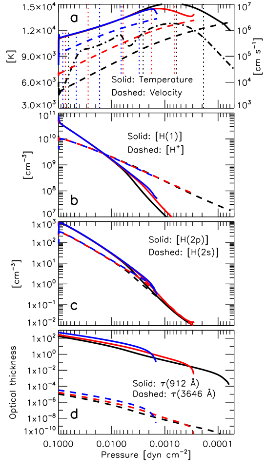
Figure 1: Model profiles. Adopted planet masses: $M_{\rm{p}}$/$M_{\rm{J}}$=2.88 (black), 2.04 (red), and 1.20 (blue). (a) Temperature and velocity; (b) H(1) and H⁺ number density; (c) H(2p) (=H(2p_1/2)+H(2p_3/2)) and H(2s) number density; (d) Optical thickness $\tau_{r\rightarrow\infty}$ at the edge of the Lyman ($<$912 Å) and Balmer ($<$3646 Å) continua. In (a) the dotted vertical lines refer to $r$/$R_{\rm{p}}$=1.02, 1.1, 1.3, 1.6, 2. Each model is run from $r$/$R_{\rm{p}}$=1 to 2.5. In (a), the dashed-dotted curve shows the temperature profile for a simulation with $M_{\rm{p}}$/$M_{\rm{J}}$=2.88 and $F^{\star}$($\lambda$$>$912 Å)$\equiv$0.

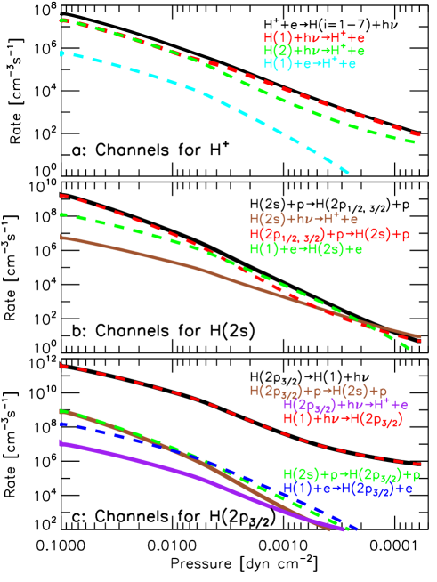
Figure 2: Channels of formation (dashed curves) and destruction (solid curves) for H⁺ (a), H(2$s$) (b) and H(2$p_{3/2}$) (c). In a, the radiative recombination channel contains products in all possible bound states, and H(2) refers to all the states with principal quantum number $n$=2. In b-c, p actually refers to collisions with both protons and electrons.

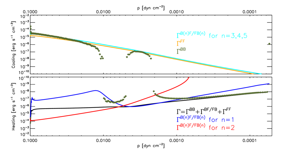
Figure 3: For the fiducial model, net energy emission rates. As defined in the text, $\Gamma$ is calculated at each altitude by integration over wavelength and solid angle with the emission and absorption coefficients specific to the designated BB, BF/FB or FF transition. Each component of $\Gamma$ can be either positive (cooling; in which case it appears in the upper panel) or negative (heating; it appears in the lower panel), and they can transition from positive to negative (or vice versa) as the specific mechanism switches from cooling to heating (or vice versa). For BF/FB transitions, there are three separate curves for processes involving the principal quantum numbers $n$=1, 2, and 3–5. The net heating ($\Gamma^{B(2)F/FB(2)}$$<$0; red curve) that occurs through the photoionization and subsequent radiative recombination H(2)+$hc$/$\lambda$ ($\lambda$$<$3,646 Å)$\leftrightarrow$ H⁺+e dominates the energy budget in the lower thermosphere.

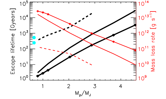
Figure 4: Escape lifetimes $t_{\rm{esc}}$ and mass loss rates $\dot{m}$. Each set of curves corresponds to a model configuration specific to KELT-9b. Dashed: $F^{\star}$($\lambda$$>$912 Å)$\equiv$0. Solid: Full stellar spectrum, orbital distance $a$=0.035 AU. Diamonds: Full stellar spectrum, $a$=0.025 AU. Cyan circles refer to simulations for HD209458b, with the low mass loss rate referring to $F^{\star}$($\lambda$$>$912 Å)$\equiv$0, and the high mass loss rate referring to the full stellar spectrum.

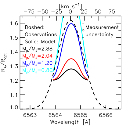
Figure 5: H-$\alpha$ transmission spectrum. Model-predicted effective size of KELT-9b at H-$\alpha$ in units of optical radius ($R_{\rm{opt}}$/$R_{\rm{J}}$=1.9) for $M_{\rm{p}}$/$M_{\rm{J}}$=2.88 (black), 2.04 (red), 1.20 (blue), and 0.80 (cyan). The synthetic spectrum considers the Doppler broadening introduced by the bulk atmospheric flow on both the day- and nightsides. The dashed line represents the available H-$\alpha$ measurements and their estimated uncertainties (Yan & Henning, 2018; Cauley et al., 2019).

Hydrodynamic model

Our hydrodynamic model solves the mass, momentum and energy conservation equations in a planetary atmosphere irradiated by its host star (García Muñoz, 2007). The model considers a gas that contains a total of $\mathcal{S}$=9 pseudo-species, and solves in a spherical geometry the conservation equations:

$$\frac{\partial\mathbf{U}}{\partial t}+\frac{\partial\mathbf{F}}{\partial r}=\mathbf{S}$$

$$\mathbf{U}=\left(\begin{array}[]{c}r^{2}\rho_{s}\\ r^{2}\rho u\\ r^{2}\rho E\end{array}\right)\qquad\mathbf{F}=\left(\begin{array}[]{c}r^{2}\rho_{s}(u+u_{s}+v_{s})\\ r^{2}(\rho u^{2}+p)\\ r^{2}(\rho E+p)u+r^{2}q\end{array}\right)\qquad\mathbf{S}=\left(\begin{array}[]{c}r^{2}\dot{\omega}_{s}\\ r^{2}\rho f_{\rm{ext}}+2pr\\ \rho ur^{2}f_{\rm{ext}}-r^{2}\Gamma\end{array}\right).$$

Here, $r$ is the radial distance to the planet center; $\rho_{s}$ is the mass density of the $s$th species, related to the number density and mass of the species through $\rho_{s}$=$n_{s}$$m_{s}$ and to the mass density of the whole gas through $\rho$=$\sum_{\mathcal{S}}\rho_{s}$; $u$ is the mass average velocity of the gas, and $u_{s}$ and $v_{s}$ are the molecular and eddy diffusion velocities of the $s$th species, respectively; $p$ is pressure; $\rho E=\rho e+\frac{1}{2}\rho u^{2}$ is the total energy of the gas, where the internal energy $\rho e$=$\sum_{\mathcal{S}}n_{s}e_{s}^{\rm{tran}}$+$\sum_{\mathcal{S}-e}n_{s}E^{\rm{exci}}_{s}$ includes contributions from the translational motion of all species ($e_{s}^{\rm{tran}}$=$\frac{3}{2}kT$) and the excitation energy above the ground state for the atoms ($E^{\rm{exci}}_{s}$); $\dot{\omega}_{s}$ is the net mass production for the $s$th species; $f_{\rm{ext}}$ is the net external force per unit of volume, which includes contributions from the planet and stellar gravitational attractions and from the planet’s centrifugal motion; $q$ is the heat flux (with contributions from thermal conduction and the transport of enthalpy by diffusion of each species); $\Gamma$ is the net energy emission rate from radiative processes.

We discretize the above conservation equations over a spatial grid from 1 to 2.5 in $r$/$R_{p}$. It comprises 260 cells of increasing size, from $\sim$30 km at the lower boundary to $\sim$3,000 km near the top. The solution near the lower boundary is strongly influenced by heating from above, which results in temperatures near $p$$\sim$0.1 dyn cm^-2 of $\sim$10,000 K, more than twice KELT-9b’s equilibrium temperature. Our choice of a bottom boundary temperature of 8,000 K aims at partly minimizing the gradient in temperature and velocity near the lower boundary seen in Fig. (1). Imposing alternative temperatures of 4,600 or 10,000 K at the bottom boundary affects the calculated mass loss rates by less than 2%. In other words, the choice of temperature there is not critical for the overall solution.

In the simulations presented here we generally placed the lower boundary of the model at a pressure of 0.1 dyn cm^-2. We did also explore the effect of shifting the lower boundary to 0.2 dyn cm^-2. For consistency, in this simulation we reduced the radial distance of the lower boundary to 1.83$R_{\rm{J}}$, which ensures that at $r$$\sim$1.89$R_{\rm{J}}$ the pressure remains $\sim$0.1 dyn cm^-2. The new simulation resulted in a mass loss rate $\sim$3% larger than in the standard setting. This small difference suggests that heating at even higher pressures will have a minor impact on the mass loss rate, and that for it to drive the escape the energy must be deposited at high enough altitude.

For the calculations, we adopted a time step of 0.2 seconds to ensure stability of the time marching scheme. This is a few times less than for similar calculations that we did without the NLTE scheme. We interpret this more stringent requirement on the time step as a consequence of the strong interaction between the hydrodynamic and radiative problems. As usual, it is convenient to initialize a calculation with a previously converged solution and gradually modify the input conditions. Solving the radiative transfer equation in the NLTE scheme takes a significant part of the total computational time, which can be of a few days on a single CPU for full convergence. To speed up the calculations, it is convenient to start with a relatively coarse spectral grid and switch later to the finer spectral grid.

NLTE scheme

Table (1) summarizes the adopted hydrogen atom model, where index $i$=1$-$7 simply specifies each bound state. We treat each bound state, the protons and the electrons as separate pseudo-species connected with one another through collisional and radiative processes. This treatment builds upon a long history of NLTE schemes for plasmas (Bates et al., 1962a, b), and more particularly on the scheme for stellar atmospheres of Munafò et al. (2017). The reader is referred to Munafò et al. (2017) for a thorough description of the fundamental collisional and radiative processes. The work of Munafò et al. (2017) assumes that the pseudo-species in the plasma follow Maxwellian distributions of velocities at two specified translational temperatures: $T_{\rm{e}}$ for electrons and $T_{\rm{h}}$ for heavy particles. Unlike in that work, our scheme assumes that a single temperature $T$=$T_{\rm{e}}$=$T_{\rm{h}}$ describes the velocities of both electrons and heavy particles, which simplifies the treatment of the energy balance. Future work should look into the impact of this simplification.

Table 1: Hydrogen atom model. Information from the NIST Bibliographic Database (Kramida, 2010).

Index	Denomination	Degeneracy	Energy
$i$		$g_{i}$	$E^{\rm{exci}}_{i}$ [eV]
1	$1s$ ${}^{2}S_{1/2}$	2	0
2	$2p$ ${}^{2}P^{*}_{1/2}$	2	10.1988061
3	$2s$ ${}^{2}S_{1/2}$	2	10.1988104
4	$2p$ ${}^{2}P^{*}_{3/2}$	4	10.1988514
5	$3$	18	12.0875051
6	$4$	32	12.7485392
7	$5$	50	13.0545016
$\infty$	Continuum, H+	$g_{\infty}$=1	$E_{\infty}$=13.5984345
$e$	Electron	$g_{e}$=2

Collisional processes

We considered excitation ($i$$\rightarrow$$j$) and de-excitation ($j$$\rightarrow$$i$) processes in collisions of bound states with electrons:

$$\mbox{H}(i)+\mbox{e}\xrightleftharpoons[k^{e}_{j\rightarrow i}\;{[\rm{cm}^{3}\rm{s}^{-1}]}]{k^{e}_{i\rightarrow j}\;{[\rm{cm}^{3}\rm{s}^{-1}]}}\mbox{H}(j)+\mbox{e},$$

as well as ionization ($i$$\rightarrow$$\infty$) processes and their reverse of three-body recombination ($\infty$$\rightarrow$$i$):

$$\mbox{H}(i)+\mbox{e}\xrightleftharpoons[k^{e}_{\infty\rightarrow i}\;{[\rm{cm}^{6}\rm{s}^{-1}]}]{k^{e}_{i\rightarrow\infty}\;{[\rm{cm}^{3}\rm{s}^{-1}]}}\mbox{H}^{+}+\mbox{e}+\mbox{e}.$$

Rate coefficients were collected from a variety of sources. For excitation (Anderson et al., 2000, 2002; Przybilla & Butler, 2004):

$$k^{e}_{i\rightarrow j}=\frac{8.63\times 10^{-6}}{g_{i}T^{1/2}}\Upsilon_{ij}\exp{\Big{\{}-\frac{E_{j}-E_{i}}{kT_{e}}}\Big{\}},$$

where $\Upsilon_{ij}$ is the Maxwell-averaged effective collision strength. $\Upsilon_{ij}$ varies moderately with temperature and for simplicity we took the values specific to $\sim$10⁴ K. From detailed balance, the de-excitation rate coefficient is:

$$k^{e}_{j\rightarrow i}=\frac{8.63\times 10^{-6}}{g_{j}T^{1/2}}\Upsilon_{ij}.$$

We adopted $\Upsilon_{ij}$ from Anderson et al. (2002) when the orbital quantum number of the bound states are specified, and from Przybilla & Butler (2004) otherwise. For collisions between degenerate states $2p$ ${}^{2}P^{*}_{1/2}$$-$$2s$ ${}^{2}S_{1/2}$ and $2s$ ${}^{2}S_{1/2}$$-$$2p$ ${}^{2}P^{*}_{3/2}$, we adopted the $\Upsilon_{ij}$ reported by Aggarwal et al. (2018).

For ionization we adopted the formulae published by Barklem (2007) for states with principal quantum number $n$$\leq$2 and those by Vriens & Smeets (1980) for $n$$>$2. We re-fitted the published formulae to expressions of the form $aT^{b}\exp{(c/T)}$ for temperatures between 4$\times$10³ and $1.4$$\times$10⁴ K, and implemented the latter. Our fits are accurate to within 20% with respect to the original formulae over the quoted temperatures. Table (2) summarizes the implemented rate coefficients for electron-collision ionization $k^{e}_{i\rightarrow\infty}$. The rate coefficients for three-body recombination ${k^{e}_{\infty\rightarrow i}}$ are related to the rate coefficients for ionization through:

$$\frac{k^{e}_{\infty\rightarrow i}}{k^{e}_{i\rightarrow\infty}}=\frac{g_{i}}{g_{e}g_{\infty}}\frac{h^{3}}{(2\pi m_{e}kT_{e})^{3/2}}\exp{\Big{\{}\frac{E_{\infty}-E_{i}}{kT_{e}}\Big{\}}},$$

where the degeneracies $g_{e}$=2 and $g_{\infty}$=1, $h$ and $k$ are the Planck and Boltzmann constants, and $m_{e}$ is the electron mass.

Table 2: Rate coefficients for electron-collision ionization. For each entry, the three numerical values specify, from top to bottom: $a$, $b$, $c$, with the rate coefficient $aT^{b}\exp{(c/T)}$ [cm³ s^-1]. Numbers in parentheses stand for exponents, i.e. 1.35($-$7) means 1.35$\times$10^-7.

Index	$k^{e}_{i\rightarrow\infty}$	Reference
$i$	[cm3 s-1]
	1.51
1	$-$2.09	Barklem (2007)
	$-$1.68(+5)
	1.35($-$7)
2–4	$-$0.033	Barklem (2007)
	$-$3.89(+4)
	1.96($-$7)
5	0.15	Vriens & Smeets (1980)
	$-$1.85(+4)
	1.27($-$6)
6	0.053	Vriens & Smeets (1980)
	$-$1.09(+4)
	5.39($-$6)
7	$-$0.023	Vriens & Smeets (1980)
	$-$7.38(+3)

The mixing of nearly-equal energy states in collisions with protons is very rapid. Thus, we considered:

$$\mbox{H}(i)+\mbox{H}^{+}\xrightleftharpoons[k^{p}_{j\rightarrow i}\;{[\rm{cm}^{3}\rm{s}^{-1}]}]{k^{p}_{i\rightarrow j}\;{[\rm{cm}^{3}\rm{s}^{-1}]}}\mbox{H}(j)+\mbox{H}^{+},$$

for the $2p$ ${}^{2}P^{*}_{1/2}$, $2s$ ${}^{2}S_{1/2}$ and $2p$ ${}^{2}P^{*}_{3/2}$ states. We adopted the rate coefficients at $T$=10⁴ K calculated by Seaton (1955), omitting the mild temperature-dependence of the process (Struensee & Cohen, 1988). Neglecting the inter-state energy separation with respect to $kT$, the reverse rates were simply estimated from the ratios of degeneracies.

The processes involving collisions with neutrals:

$$\mbox{H}(i)+\mbox{H}(n=1)\rightleftharpoons\mbox{H}(j)+\mbox{H}(n=1)$$

$$\mbox{H}(i)+\mbox{H}(n=1)\rightleftharpoons\mbox{H}^{+}+\mbox{e}+\mbox{H}(n=1)$$

are outpaced by their electron-collision counterparts even for small ionization fractions of $\sim$10^-4 (Colonna et al., 2012; Munafò et al., 2017). These processes are safely neglected for the conditions of KELT-9b’s thermosphere.

Collisional processes contribute to the population of bound states, protons and electrons through the corresponding mass production terms $\dot{\omega}_{i}$, $\dot{\omega}_{\rm{H}^{+}}$, and $\dot{\omega}_{e}$ in the gas continuity equations.

Radiative processes

Our NLTE scheme considers bound-bound (BB), bound-free/free-bound (BF/FB) and free-free (FF) radiative transitions. These processes couple the radiation field with the population of hydrogen atom states, and introduce non-local effects as photons diffuse through the atmosphere from where they are emitted to where they are ultimately absorbed. In our treatment, we omitted the process of induced emission in BB and BF/FB transitions because its effect is minor.

BB transitions

We considered photoexcitation between bound states by absorption:

$$\mbox{H}(i)+hc/\lambda_{ij}\xrightarrow[]{(B_{ij}\lambda^{2}_{ij}/c)\Phi_{ij}\;{[\rm{s}^{-1}]}}\mbox{H}(j)$$

and spontaneous emission:

$$\mbox{H}(j)\xrightarrow[]{A_{ji}\;{[\rm{s}^{-1}]}}\mbox{H}(i)+hc/\lambda_{ij}.$$

$c$ is the speed of light and $\lambda_{ij}$=$hc$/($E_{j}$$-$$E_{i}$) the line wavelength. $B_{ij}$ and $A_{ji}$ are the Einstein coefficients for absorption and spontaneous emission, related through:

$$B_{ij}=\frac{g_{j}}{g_{i}}\frac{\lambda^{3}_{ij}}{2hc}A_{ji}.$$

$\Phi_{ij}$=$\int\mathcal{J}_{\lambda}\psi^{ij}_{\lambda}d\lambda$ [erg cm^-2s^-1sr^-1cm^-1] is the integral of the local average intensity $\mathcal{J}_{\lambda}$ (see below) over the transition line profile $\psi^{ij}_{\lambda}(\lambda)$ (normalized to $\int_{0}^{\infty}\psi^{ij}_{\lambda}(\lambda)d\lambda$=1). We assume complete frequency redistribution, and thus the line profiles for absorption and emission satisfy $\psi^{ij}_{\lambda}(\lambda)=\psi^{ji}_{\lambda}(\lambda)$. We model $\psi^{ij}_{\lambda}(\lambda)$ as a Voigt function obtained from the convolution of Gaussian and Lorentz functions, and use the analytical approximations given by Whiting (1968). Thermal broadening contributes to the Gaussian component, and natural and Stark broadening contribute to the Lorentz component. Our implementation of Stark broadening is based on low pressure plasmas (Griem, 1974; Kramida et al., 2018). For computational expediency, we considered for photoexcitation and in the radiative transfer solution only the Lyman-$\alpha$ line that pumps ground state atoms into the excited states $2p$ ${}^{2}P^{*}_{1/2}$ and $2p$ ${}^{2}P^{*}_{3/2}$. This approximation is adequate to describe the population of excited states with principal quantum number $n$=2, which is the focus of our work. All the other lines are not considered for photoexcitation or in the radiative transfer problem. We do consider however the effect of spontaneous emission of all BB transitions in the energy balance by considering that the emission lines other than Lyman-$\alpha$ are optically transparent and thus the corresponding radiated energy escapes the atmosphere. That absorption in Lyman-$\alpha$ is more important than in the other -$\beta$, -$\gamma$, -$\delta$, etc., lines of the Balmer series is justified by the combination of decreasing values for the corresponding $B_{1j}$ Einstein coefficients and the drop of stellar emission towards shorter wavelengths.

We expect that a more complete treatment of all BB transitions will increase to some extent the population of $n$=2 states, as the states with $n$$>$2 will cascade through $n$=2. We also expect that solving the radiative transfer problem in all the lines, i.e. moving away from the assumption of transparency for all lines except Lyman-$\alpha$, will increase the energy deposited in the thermosphere. Either way, these changes – which will be implemented in future work – will reinforce the mechanism that sustains the proposed Balmer-driven escape.

For BB transitions, the emission $\varepsilon^{\rm{BB}}_{\lambda}$ [erg cm^-3s^-1sr^-1cm^-1] and absorption $\kappa^{\rm{BB}}_{\lambda}$ [cm^-1] coefficients that enter the radiative transfer equation are generally given by:

$$\varepsilon^{\rm{BB}}_{\lambda}=\sum_{j>i}\frac{hc}{4\pi\lambda_{ij}}n_{j}A_{ji}\psi^{ij}_{\lambda}$$

$$\kappa^{\rm{BB}}_{\lambda}=\sum_{j>i}\frac{h\lambda_{ij}}{4\pi}n_{i}B_{ij}\psi^{ij}_{\lambda},$$

where $n_{i}$ is the number density of bound state $i$, and $\kappa^{\rm{BB}}_{\lambda}$ omits the typically small contribution from induced emission. In our treatment, we use the above expressions for $\varepsilon^{\rm{BB}}_{\lambda}$ and $\kappa^{\rm{BB}}_{\lambda}$ only for Lyman-$\alpha$. For the other lines, we take $\kappa^{\rm{BB}}_{\lambda}$$\approx$0 and simply include the wavelength-integrated form of $\varepsilon^{\rm{BB}}_{\lambda}$ in the net energy emission rate $\Gamma$.

Our adopted Einstein coefficients are based on transition probabilities and wavelengths from the NIST Bibliographic Database (Kramida et al., 2018).

BF/FB transitions

We considered photoionization of bound states:

$$\mbox{H}(i)+hc/\lambda(>E_{\infty}-E_{i})\xrightarrow[]{J_{i\rightarrow\infty}\;{[\rm{s}^{-1}]}}\mbox{H}^{+}+\mbox{e}$$

and spontaneous radiative recombination:

$$\mbox{H}^{+}+\mbox{e}\xrightarrow[]{k^{rr}_{\infty\rightarrow i}\;{[\rm{cm}^{3}\rm{s}^{-1}]}}\mbox{H}(i)+hc/\lambda(>E_{\infty}-E_{i}).$$

For BF/FB transitions, we calculated the emission and absorption coefficients from:

$$\varepsilon^{\rm{FB}}_{\lambda}=\frac{h^{4}c^{2}n_{e}n_{\rm{H}^{+}}}{\lambda^{5}(2\pi m_{e}kT_{e})^{3/2}}\times\sum_{i}\sigma_{i}^{\rm{PI}}(\lambda)\frac{g_{i}}{g_{\infty}}\exp{\Big{\{}\frac{E_{\infty}-E_{i}}{kT_{e}}}-\frac{hc/\lambda}{kT_{e}}\Big{\}}$$

$$\kappa^{\rm{BF}}_{\lambda}=\sum_{i}\sigma_{i}^{\rm{PI}}(\lambda)n_{i}.$$

$\kappa^{\rm{BF}}_{\lambda}$ neglects the small contribution from induced radiative recombination. We calculated the photoionization cross sections $\sigma_{i}^{\rm{PI}}(\lambda)$ with the analytical formula for hydrogenic atoms given by Mihalas (1978) (pp. 99, Eq. 4-114), and omitted the small corrections from the bound-free Gaunt factors.

The rate coefficient for photoionizaton is calculated as:

$$J_{i\rightarrow\infty}=\frac{4\pi}{hc}\int\sigma_{i}^{\rm{PI}}(\lambda)\mathcal{J}_{\lambda}(\lambda)\lambda d\lambda,$$

and for spontaneous radiative recombination:

$$k^{rr}_{\infty\rightarrow i}=\sqrt{\frac{2}{\pi}}\frac{g_{i}}{g_{\infty}}\frac{h^{3}c}{(m_{e}kT_{e})^{3/2}}\exp{\Big{\{}\frac{E_{\infty}-E_{i}}{kT_{e}}}\Big{\}}\int\frac{\sigma_{i}^{\rm{PI}}(\lambda)}{\lambda^{4}}\exp{\Big{\{}-\frac{hc/\lambda}{kT_{e}}}\Big{\}}d\lambda.$$

We integrated numerically $k^{rr}_{\infty\rightarrow i}$ and fitted the resulting rate coefficients at temperatures of 10³–2$\times$10⁴ K to the expression $aT^{b}\exp{(c/T)}$. Radiative recombination readily populates highly excited states. Because our atom model is truncated at the principal quantum number $n$=5, we calculated the rate coefficients up to $n$$\sim$40 and added the net difference for channels above $n$=4 to our channel with $n$=5, thus ensuring that the net recombination of protons and electrons occurs at the proper rate. Table (3) lists the photoionization rate coefficients at the top of the atmosphere for our choice of stellar spectrum. Figure (1) shows the variation of the photoionization rate coefficients with altitude, together with the rate coefficients $(B_{ij}\lambda^{2}_{ij}/c)\Phi_{ij}$ for photoexcitation $1s$ ${}^{2}S_{1/2}$$\rightarrow$$2p$ ${}^{2}P^{*}_{1/2}$ and $1s$ ${}^{2}S_{1/2}$$\rightarrow$$2p$ ${}^{2}P^{*}_{3/2}$.

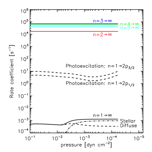
Figure 1: Photoionization and photoexcitation rate coefficients. For photoionization of H(1), the dotted-dashed and dashed lines distinguish the separate contributions from stellar and diffuse radiation.

Table 3: Photoionization rate coefficient at the top of the atmosphere.

Principal quantum number	${J_{n\rightarrow\infty}}$
$n$	[s-1]
1	1.34($-$3)
2	1.70($+$4)
3	7.03($+$4)
4	5.73($+$4)
5	3.99($+$4)

FF transitions

For FF transitions the emission and absorption coefficients are:

$$\varepsilon^{\rm{FF}}_{\lambda}=\frac{8}{3}\sqrt{\frac{2\pi}{3m_{e}kT_{e}}}\frac{n_{e}n_{\rm{H}^{+}}q^{6}_{\rm{e}}}{\lambda^{2}m_{e}c^{2}}\exp{\Big{\{}-\frac{hc/\lambda}{kT_{e}}}\Big{\}}$$

$$\kappa^{\rm{FF}}_{\lambda}=\frac{4}{3}\sqrt{\frac{2\pi}{3m_{e}kT_{e}}}\frac{\lambda^{3}n_{e}n_{\rm{H}^{+}}q^{6}_{\rm{e}}}{m_{e}hc^{4}}\Big{[}1-\exp{\Big{\{}-\frac{hc/\lambda}{kT_{e}}}\Big{\}}\Big{]}$$

where $q_{e}$=4.8032068$\times$10^-10 esu is the electron charge in cgs units.

Contribution to populations

BB and BF/FB transitions contribute to the population of bound states, protons and electrons through the corresponding mass production terms $\dot{\omega}_{i}$, $\dot{\omega}_{\rm{H}^{+}}$, and $\dot{\omega}_{e}$.

Radiative transfer

We solve the radiative transfer equation:

$$\frac{dI_{\lambda}}{ds}=-\kappa_{\lambda}I_{\lambda}+\varepsilon_{\lambda},$$

which does not explicitly include a scattering term, although scattering occurs both in BB and BF/FB transitions. For instance at Lyman-$\alpha$ a photon emitted in the optically thick line will be reabsorbed immediately after, which will lead to a new reemission. Also, absorption of energetic photons will ionize the neutral gas, the products of which will recombine and reemit a fraction of the initially absorbed radiation. Each new absorption-emission event is effectively a scattering event. The above equation also does not explicitly consider the redistribution of photons in wavelength by e.g. the Doppler shift induced by the thermal motion of atoms or the bulk gas motion. Although these effects will modify aspects of the radiation field such as the penetration of photons in the thermosphere (Huang et al., 2017), their rigorous treatment in the framework of our hydrodynamics-NLTE model is currently impractical.

We solve the radiative transfer equation in a plane-parallel atmosphere along the substellar line (Fig. 2), obtaining the radiance $I_{\lambda}$$(\mathbf{x,s})$ [erg cm^-2s^-1sr^-1cm^-1]. The solution to the radiative transfer equation at a location $\mathbf{x}$ for radiation coming from direction $-\mathbf{s}$ is:

$$I_{\lambda}(\mathbf{x,s})=I_{\lambda}^{\star}(\mathbf{x,s})+I_{\lambda}^{\rm{d}}(\mathbf{x,s})=\mathcal{F}^{\star}_{\lambda}\exp{(-\tau_{\lambda}(\mathbf{x}\rightarrow\mathbf{x}_{\star}))}\delta(\mathbf{s}-\mathbf{s}_{\star})+\int_{\mathbf{x}}^{\infty}S_{\lambda}(\mathbf{x^{\prime}})\exp{(-\tau_{\lambda}(\mathbf{x}\rightarrow\mathbf{x^{\prime}}))}d\tau_{\lambda}(\mathbf{x^{\prime}}).$$ (1)

$I_{\lambda}^{\star}(\mathbf{x,s})$ represents the non-diffuse radiance associated with the stellar irradiance $\mathcal{F}^{\star}_{\lambda}$ [erg cm^-2 s^-1 cm^-1] at the planet’s orbit that is attenuated through the atmosphere. $I_{\lambda}^{\star}(\mathbf{x,s})$ is zero for all directions except for the direction towards the star $\mathbf{s}_{\star}$. $\delta(\mathbf{s}-\mathbf{s}_{\star})$ is the Dirac delta function centered at $\mathbf{s}_{\star}$ and by definition $\int\delta(\mathbf{s}-\mathbf{s}_{\star})d\Omega(\mathbf{s})$=1. $I_{\lambda}^{\rm{d}}(\mathbf{x,s})$ represents the diffuse radiance that arises within the atmosphere due to BB, FB and FF emission, $d\tau_{\lambda}(\mathbf{x^{\prime}})$=$\kappa_{\lambda}(\mathbf{x^{\prime}})d\ell$ and $\ell$=$\|\mathbf{x}-\mathbf{x^{\prime}}\|$. $S_{\lambda}(\mathbf{x})$=$\varepsilon_{\lambda}(\mathbf{x})$/$\kappa_{\lambda}(\mathbf{x})$ is the source function. One could conceive an additional contribution to $I_{\lambda}(\mathbf{x,s})$ from radiation originating below the thermosphere, but we confirmed that this contribution is negligible.

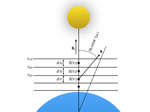
Figure 2: The radiative transfer equation is solved in the approximation of plane-parallel atmosphere. The diffuse radiances $I^{\rm{d}}_{\lambda}(\mathbf{x,\mu}_{k})$ are solved along multiple directions specified by the angle $\Theta_{k}$ and integrated in solid angle to obtain the diffuse average intensity $\mathcal{J}^{\rm{d}}_{\lambda}$.

The average intensity $\mathcal{J}_{\lambda}(\mathbf{x})$ (same units as $I_{\lambda}(\mathbf{x,s})$) that contributes to various BB and BF/FB processes is defined as the integral of radiance over solid angle $\Omega(\mathbf{s})$:

$$\mathcal{J}_{\lambda}(\mathbf{x})=\frac{1}{4\pi}\int I_{\lambda}(\mathbf{x},\mathbf{s})d\Omega(\mathbf{s}).$$

For the stellar contribution:

$$\mathcal{J}^{\star}_{\lambda}(\mathbf{x})=\frac{\mathcal{F}^{\star}_{\lambda}}{4\pi}\exp{(-\tau_{\lambda}(\mathbf{x}\rightarrow\mathbf{x}_{\star}))}.$$

The expression for $I_{\lambda}^{\rm{d}}(\mathbf{x,s})$ is a line integral that can be evaluated once the gas properties are specified. To capture the directionality of diffuse radiation, $I_{\lambda}^{\rm{d}}(\mathbf{x,s})$ is calculated at $n_{\mu}$ evenly-separated directions $\mu_{k}$=$\mathbf{s}_{k}\cdot\mathbf{u_{r}}$=$\cos{\Theta_{k}}$=$-1$+2/$n_{\mu}$$\times$($k$$-$1/2) and $k$=1, …, $n_{\mu}$. We numerically calculate the diffuse average intensity as:

$$\mathcal{J}^{\rm{d}}_{\lambda}(\mathbf{x})=\frac{1}{4\pi}\int I^{\rm{d}}_{\lambda}(\mathbf{x},\mathbf{s})d\Omega(\mathbf{s})=\frac{1}{n_{\mu}}\sum_{k=1}^{n_{\mu}}I^{\rm{d}}_{\lambda}(\mathbf{x,\mu}_{k}).$$

We take $n_{\mu}$=4, which represents two upward and two downward directions, which is a good trade-off between computational expediency and accuracy. Both $\mathcal{J}^{\star}_{\lambda}$ and $\mathcal{J}^{\rm{d}}_{\lambda}$ vary through the atmosphere, as seen in Fig. (3). Diffuse radiation plays the fundamental role of transferring energy between altitudes.

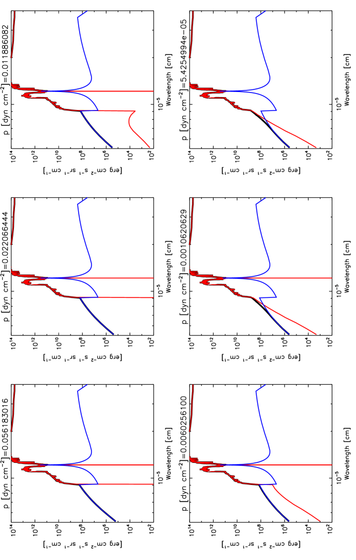
Figure 3: For the fiducial model, average intensity ($\mathcal{J}_{\lambda}$; black) and contributions from the star ($\mathcal{J}^{\star}_{\lambda}$; red) and from diffuse radiation ($\mathcal{J}^{\rm{d}}_{\lambda}$; blue) at the specified pressure levels.

Numerical solution to the radiative transfer equation

The solution for the non-diffuse radiance $I_{\lambda}^{\star}(\mathbf{x,s})$ is trivial and given by Beer-Lambert’s law. To solve for the diffuse radiance $I_{\lambda}^{\rm{d}}(\mathbf{x,s})$ we choose to recast the radiative transfer equation as:

$$\frac{dI^{\rm{d}}_{\lambda}}{d(\tau_{\lambda}/\mu_{k})}=-I^{\rm{d}}_{\lambda}+S_{\lambda},$$

where $S_{\lambda}=\varepsilon_{\lambda}/\kappa_{\lambda}$ is the source function, $\tau_{\lambda}$ is the optical thickness in the substellar direction and $\mu_{k}$ defines the orientation of the radiation ray (Fig. 2). The formal solution to this equation with a zero-influx at the boundary is:

$$I^{\rm{d}}_{\lambda}=\int_{0}^{\infty}S_{\lambda}(\tau)\exp{(-\tau/\mu_{k})}d(\tau/\mu_{k}),$$

which represents the source function weighted by the transmittance of the gas column. $S_{\lambda}(\tau)$ varies slowly with $\tau$ even when the optical thickness changes rapidly. Numerically, we approximate:

$$I^{\rm{d}}_{\lambda}\approx S_{\lambda}(\tau_{1}=0)\int_{\tau_{1}=0}^{\tau_{3/2}}\exp{(-\tau/\mu_{k})}d(\tau/\mu_{k})+\sum_{l>1}S_{\lambda}(\tau_{l})\int_{\tau_{l-1/2}}^{\tau_{l+1/2}}\exp{(-\tau/\mu_{k})}d(\tau/\mu_{k})=$$

$$S_{\lambda}(\tau_{1}=0)[1-\exp(-\Delta\tau_{1}/2/\mu_{k})]+\sum_{l>1}S_{\lambda}(\tau_{l})\exp{(-\tau_{l-1/2}/\mu_{k})}[1-\exp(-\Delta\tau_{l}/\mu_{k})]$$

which assumes that the source function is constant within each atmospheric slab and where index $l$ runs over all the slabs starting from the local position along the specified $\mathbf{s}$ direction.

The radiative transfer equation is solved over a non-uniform spectral grid of 751 bins, shown by the green bars of Fig. (4). It resolves the Lyman-$\alpha$ line in great detail with a minimum bin size at the line core equal to 0.1$\times$ the full width at half maximum (FWHM) for Doppler (thermal) broadening. In the Lyman continuum the spectral bins are 10-50 Å wide, whereas longwards of $\sim$1,500 Å they are $\sim$300 Å wide or larger. We tested whether our findings were sensitive to the choice of spectral grid, and in particular to the details near the Lyman-$\alpha$ line. In our tests, we always used a minimum bin size at the line core of (0.1–0.2)$\times$the Doppler FWHM. For the region $\sim$1216$\pm$300 Å, we experimented with bin sizes $\Delta$$\lambda$_p that increase towards both the shorter and longer wavelengths, i.e. $\Delta$$\lambda$_p+1=$\Delta$$\lambda$_p$\times$$r_{\rm{stretch}}$, where $\Delta$$\lambda$₀ is the (minimum) bin size at the Lyman-$\alpha$ core. We used stretching factors $r_{\rm{stretch}}$ ranging from $\sim$1.40 (coarse grid) to $\sim$1.01 (fine grid). This translates into grids that contain from 100 to 750 bins. Over all these sensitivity experiments, the calculated mass loss rate for our fiducial case varied by less than 15%. The calculations presented here use $r_{\rm{stretch}}$$\sim$1.01 and $\Delta$$\lambda$₀=0.1$\times$Doppler FWHM.

Stellar irradiation

For our model simulations, we implemented the PHOENIX spectrum shown in Fig. (4) (Husser et al., 2013). It has an EUV-integrated irradiance $F^{\star}_{\rm{LyC}}$=$\int_{\lambda<912{\textup{\AA}}}\mathcal{F}^{\star}_{\lambda}d\lambda$=3.8 (3,100) erg s^-1cm^-2 at 1 (0.035) AU. The EUV energy is orders of magnitude less than $F^{\star}_{\rm{BaC}}$=$\int_{\lambda<3646{\textup{\AA}}}\mathcal{F}^{\star}_{\lambda}d\lambda$=2.9$\times$10⁷ erg s^-1cm^-2 (1 AU), which results in $F^{\star}_{\rm{BaC}}$/$F^{\star}_{\rm{LyC}}$$\sim$7.5$\times$10⁶. Figure (3) shows the stellar average intensity $\mathcal{J}^{\star}_{\lambda}$ (red curves) in the adopted spectral grid of our model. At very high altitudes with negligible absorption $\mathcal{J}^{\star}_{\lambda}$$\approx$ $\mathcal{F}^{\star}_{\lambda}$/4$\pi$.

Details in the stellar model such as temperature structure, chemical abundances or the LTE/NLTE treatment of the radiation problem will surely affect the estimated EUV output of KELT-9. Our work shows though that KELT-9b’s thermospheric structure is largely dictated by energy deposition in the Balmer continuum. As a result, uncertainties in KELT-9’s EUV spectrum by a factor of up to a few have a negligible impact on the planet thermosphere. We moreover confirm that for our fiducial model, increasing the stellar EUV spectrum by $\times$6 produces a change in the mass loss rate $\dot{m}$$<$3%.

Numerical integration

The hydrodynamic and NLTE problems are strongly coupled and must be solved self-consistently. In our implementation, we proceed sequentially by calculating the radiation field on the basis of the best estimate of atmospheric properties at the time. The outcome of this step is the average intensity $\mathcal{J}_{\lambda}(\mathbf{x})$ at each location along the substellar line. Having calculated the radiation field, the hydrodynamics and NLTE equations are solved, enabling us to re-estimate the radiation field. This iterative procedure is repeated until convergence of all the variables in the radiation, population and hydrodynamics problems.

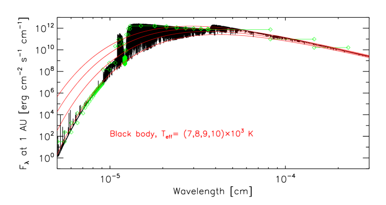
Figure 4: PHOENIX spectrum adopted for KELT-9 (Husser et al., 2013). For reference, black body emissions at the specified temperatures are also shown. The green bars show the implemented lower-resolution spectrum.

Breakdown of net energy emission rates in the fiducial model

By construction, the net energy emission rate that goes into the energy conservation equation is:

$$\Gamma(\mathbf{x})=\Gamma^{\rm{BB}}(\mathbf{x})+\Gamma^{\rm{BF/FB}}(\mathbf{x})+\Gamma^{\rm{FF}}(\mathbf{x}),$$

which contains contributions from BB, BF/FB and FF transitions.

In our treatment of BB transitions, we assume that all lines except Lyman-$\alpha$ are transparent, and thus:

$$\Gamma^{\rm{BB}}(\mathbf{x})\approx 4\pi\int[-\kappa^{\rm{Ly-}\alpha}_{\lambda}(\mathbf{x})\mathcal{J}_{\lambda}(\mathbf{x})+\varepsilon^{\rm{Ly-}\alpha}_{\lambda}(\mathbf{x})]d\lambda+\sum_{j>i,\rm{except\;Ly-}\alpha}\frac{hc}{\lambda_{ij}}n_{j}A_{ji}.$$

For BF/FB transitions, we consider separate contributions from each bound state with principal quantum number $n$:

$$\Gamma^{\rm{B(n)F/FB(n)}}(\mathbf{x})=4\pi\int[-\kappa^{\rm{B(n)F}}_{\lambda}(\mathbf{x})\mathcal{J}_{\lambda}(\mathbf{x})+\varepsilon^{\rm{FB(n)}}_{\lambda}(\mathbf{x})]d\lambda.$$

The BF/FB contributions involving $n$=1 and 2 dominate the overall energy budget. H(1) dominates in the upper thermosphere whereas H(2) dominates in the lower thermosphere.

Finally, for FF transitions:

$$\Gamma^{\rm{FF}}(\mathbf{x})=4\pi\int[-\kappa^{\rm{FF}}_{\lambda}(\mathbf{x})\mathcal{J}_{\lambda}(\mathbf{x})+\varepsilon^{\rm{FF}}_{\lambda}(\mathbf{x})]d\lambda.$$

References

- Ballester & Ben-Jaffel (2015) Ballester, G.E. & Ben-Jaffel, L. 2015, ApJ, 804:116
- Ben-Jaffel (2007) Ben-Jaffel, L. 2007, ApJ, 671:L61-L64
- Bourrier et al. (2018) Bourrier, V., Lecavelier des Etangs, A., Ehrenreich, D., Sanz-Forcada, J., Allart, R., et al. 2018, A&A, 620:A147
- Cauley et al. (2019) Cauley, P.W., Shkolnik, E.L., Ilyin, I., Strassmeier, K.G., Redfield, S. & Jensen, A. 2019, AJ, 157:69
- Casasayas-Barris et al. (2018) Casasayas-Barris, N., Pallé, E., Yan, F., Chen, G., Albrecht, S., et al. 2018, A&A, 616:A151
- Christie et al. (2013) Christie, D., Arras, P. & Li, Z.-Y. 2013, ApJ, 772:144
- Collier Cameron et al. (2010) Collier Cameron, A., Guenther, E., Smalley, B., McDonald, I., Hebb, L., et al. 2010, MNRAS, 407:507
- Debrecht et al. (2019) Debrecht, A., Carroll-Nellenback, J., Frank, A., McCann, J., Murray-Clay, R. & Blackman, E.G. 2019, MNRAS, 483:1481–1495
- Ehrenreich et al. (2015) Ehrenreich, D., Bourrier, V., Wheatley, P.J., Lecavelier des Etangs, A., Hébrard, G. 2015, Nature, 522:459
- Fossati et al. (2010) Fossati, L., Haswell, C.A., Froning, C.S., Hebb, L., Holmes, S., et al. 2010, ApJ, 714:L222
- Fossati et al. (2018) Fossati, L., Koskinen, T., Lothringer, J.D., France, K., Young, M.E. & Sreejith, A.G. 2018, ApJ, 868:L30
- Fulton et al. (2017) Fulton, B.J., Petigura, E.A., Howard, A.W., Isaacson, H., Marcy, G.W., et al. 2017, ApJ, 154:109
- García Muñoz (2007) García Muñoz, A. 2007, Planet. Space Science, 55:1426
- Gaudi et al. (2017) Gaudi, B.S., Stassun, K.G., Collins, K.A., Beatty, T.G., Zhou, G., et al. 2017, Nature, 546:514
- Gnat & Ferland (2002) Gnat, O. & Ferland, G.J. 2012, ApJS, 199:20
- Guo & Ben-Jaffel (2016) Guo, J.H. & Ben-Jaffel, L. 2016, ApJ, 818:107
- Hoeijmakers et al. (2018) Hoeijmakers, H.J., Ehrenreich, D., Heng, K., Kitzmann, D., Grimm, S.L., et al. 2018, Nature, 560:453
- Hoeijmakers et al. (2019) Hoeijmakers, H.J., Ehrenreich, D., Kitzmann, D., Allart, R., Grimm, S.L., et al. 2019, A&A, in press
- Huang et al. (2017) Huang, C., Arras, P., Christie, D. & Li, Z.-Y. 2017, ApJ, 851:150
- Husser et al. (2013) Husser, T.-O., Wende-von Berg, S., Dreizler, S., Homeier, D., Reiners, A., et al. 2013, A&A, 553:A6
- Ionov et al. (2014) Ionov, D.E., Bisikalo, D.V., Shematovich, V.I. & Huber, B. 2014, Solar System Research, 48:105
- Jensen et al. (2012) Jensen, A.G., Redfield, S., Endl, M., Cochran, W.D., Koesterke, L. & Barman, T. 2012, ApJ, 751:86
- Jin & Mordasini (2018) Jin, S. & Mordasini, C. 2018, ApJ, 853:163
- Kitzmann et al. (2018) Kitzmann, D., Heng, K., Rimmer, P.B., Hoeijmakers, H.J., Tsai, S.-M., et al. 2018, ApJ, 863:183
- Koskinen et al. (2013) Koskinen, T.T., Harris, M.J., Yelle, R.V. & Lavvas, P. 2013, Icarus, 226, 2, 1678–1694
- Kulow et al. (2014) Kulow, J.R., France, K., Linsky, J. & Loyd, R.O.P. 2014, ApJ, 786:132
- Lammer et al. (2003) Lammer, H., Selsis, F., Ribas, I., Guinan, E.F., Bauer, S.J. & Weiss, W.W. 2003, ApJ, 598:L121
- Lammer et al. (2008) Lammer, H., Kasting, J.F., Chassefière, E., Johnson, R.E., Kulikov, Y.N. & Tian, F. 2008, Space Sci. Rev., 139:399
- Lopez et al. (2012) Lopez, E.D., Fortney, J.J. & Miller, N. 2012, ApJ, 761:59
- Lothringer et al. (2018) Lothringer, J.D., Barman, T. & Koskinen, T. 2018, ApJ, 866:27
- Lecavelier des Etangs et al. (2010) Lecavelier Des Etangs, A., Ehrenreich, D., Vidal-Madjar, A., Ballester, G.E., Désert, J.-M., et al. 2010, A&A, 514:A72
- Linsky et al. (2010) Linsky, J.L., Yang, H., France, K., Froning, C.S., Green, J.C., et al. 2010, ApJ, 717:1291
- Lund et al. (2017) Lund, M.B., Rodriguez, J.E., Zhou, G., Gaudi, B.S., Stassun, K.G., et al. 2017, AJ, 154:194
- Menager et al. (2013) Menager, H., Barthélemy, M., Koskinen, T., Lilensten, J., Ehrenreich, D. & Parkinson, C.D. 2013, Icarus, 226:1709
- Munafò et al. (2017) Munafò, A., Mansour, N.N. & Panesi, M. 2017, ApJ, 838:126
- Murray-Clay et al. (2009) Murray-Clay, R.A., Chiang, E.I. & Murray, N. 2009, ApJ, 693:23
- Owen (2019) Owen, J.E. 2019, Annu. Rev. Earth Planet. Sci., 47:67
- Salz et al. (2016) Salz, M., Czesla, S., Schneider, P.C. & Schmitt, J.H.M.M. 2016, A&A, 586:A75
- Salz et al. (2018) Salz, M., Czesla, S., Schneider, P.C., Nagel, E., Schmitt, J.H.M.M., et al. 2018, A&A, 620:A97
- Schöll et al. (2016) Schöll, M., Dudok de Wit, T., Kretzschmar, M. & Haberreiter, M. 2016, J. Space Weather Space Clim., 6:A14
- Shaikhislamov et al. (2018) Shaikhislamov, I.F., Khodachenko, M.L., Lammer, H., Berezutsky, A.G., Miroshnichenko, I.B. & Rumenskikh, M.S. 2018, MNRAS, 481:5315
- Sing et al. (2019) Sing, D.K., Lavvas, P., Ballester, G.E., Lecavelier des Etangs, A., Marley, M.S., et al. 2019, AJ, 158:91
- Spake et al. (2018) Spake, J.J., Sing, D.K., Evans, T.M., Oklopčić, A., Bourrier, V., et al. 2018, Nature, 557:68
- Talens et al. (2018) Talens, G.J.J., Justesen, A.B., Albrecht, S., McCormac, J., Van Eylen, V., et al. 2018, A&A, 612:A57
- Thuillier et al. (2004) Thuillier, G., Floyd, L., Woods, T.N., Cebula, R., Hilsenrath, E., Hersé, M., & Labs, D. 2004, Solar irradiance reference spectra. In: J.M. Pap, P. Fox, C. Frohlich, H.S. Hudson, J. Kuhn, J. McCormack, G. North, W. Sprigg, and S.T. Wu, Editors. Solar variability and its effects on climate, Geophysical Monograph 141, American Geophysical Union, Washington, DC, 171.
- Tian et al. (2005) Tian, F., Toon, O.B., Pavlov, A.A. & De Sterck, H. 2005, ApJ, 621:1049
- Tian (2015) Tian, F. 2015, Annu. Rev. Earth Planet. Sci., 43:459
- Trammell et al. (2014) Trammell, G.B., Li, Z.-Y. & Arras, P. 2014, ApJ, 788:161
- Tremblin & Chiang (2013) Tremblin, P. & Chiang, E. 2013, MNRAS, 428:2565
- Vidal-Madjar et al. (2003) Vidal-Madjar, A., Lecavelier des Etangs, A., Désert, J.-M., Ballester, G.E., Ferlet, R., Hébrard, G. & Mayor, M. 2003, Nature, 422:143
- Vidal-Madjar et al. (2004) Vidal-Madjar, A., Désert, J.-M., Lecavelier des Etangs, A., Hébrard, G., Ballester, G.E., et al. 2004, ApJ, 604:L69
- Yan & Henning (2018) Yan, F. & Henning, T. 2018, Nature Astronomy, 2:714
- Wang et al. (2014) Wang, Y., Ferland, G.J., Lykins, M., Porter, R., van Hoof, P.A.M. & Williams, R.J.R. 2014, MNRAS, 440:3100
- Yelle (2004) Yelle, R.V. 2004, Icarus, 170:167
- Zahnle & Catling (2017) Zahnle, K.J. & Catling, D.C. 2017, ApJ, 843:122

References

- Le Teuff et al. (2000) Le Teuff, Y.H., Millar, T.J. & Markwick, A.J. 2000, A&A Suppl. Ser., 146, 157
- Bates et al. (1962a) Bates, D. R., Kingston, A.E. & McWhirter, R.W.P 1962, RSPSA, 267, 297
- Bates et al. (1962b) Bates, D. R., Kingston, A.E. & McWhirter, R.W.P 1962, RSPSA, 270, 155
- Kramida (2010) Kramida, A. 2010, Atomic Energy Levels and Spectra Bibliographic Database (version 2.0). Available: https://physics.nist.gov. DOI: 10.18434/T40K53.
- Anderson et al. (2000) Anderson, H., Ballance, C.P., Badnell, N.R. & Summers, H.P. 2000, J. Phys. B: At. Mol. Opt. Phys., 33, 1255
- Anderson et al. (2002) Anderson, H., Ballance, C.P., Badnell, N.R. & Summers, H.P. 2002, J. Phys. B: At. Mol. Opt. Phys., 35, 1613
- Przybilla & Butler (2004) Przybilla, N. & Butler, K. 2004, ApJ, 09:1181
- Aggarwal et al. (2018) Aggarwal, K.M., Owada, R. & Igarashi, A. 2018, Atoms, 6, 37
- Barklem (2007) Barklem, P.S. 2007, A&A, 466, 327
- Vriens & Smeets (1980) Vriens, L. & Smeets, A.H.M. 1980, Phys. Rev. A, 22, 940
- Seaton (1955) Seaton, M.J. 1955, Proc. Phys. Soc. A, 68, 457
- Struensee & Cohen (1988) Struensee, M.C. & Cohen, J.S. 1988, Phys. Rev. A, 38, 3377
- Colonna et al. (2012) Colonna, G., Pietanza, L.D. & D’Ammando, G.D. 2012, Chem. Phys., 398, 37
- Whiting (1968) Whiting, E.E. 1968, JQSRT, 8, 1379
- Griem (1974) Griem, H.R. 1974, Spectral Line Broadening by Plasmas, Academic Press, New York and London.
- Kramida et al. (2018) Kramida, A., Ralchenko, Yu., Reader, J., & NIST ASD Team 2018. NIST Atomic Spectra Database (ver. 5.5.6), [Online]. Available: https://physics.nist.gov/asd. DOI: https://doi.org/10.18434/T4W30F
- Nussbaumer & Schmutz (1984) Nussbaumer, H. & Schmutz, W. 1984, A&A, 138, 495
- Dennison et al. (2005) Dennison, B., Turner, B.E. & Minter, A.H. 2005, ApJ, 633, 309
- Mihalas (1978) Mihalas, D. 1978, Stellar Atmospheres, 2nd Edition, W.H. Freeman and Company, San Francisco.