Probing the Electroweak Sphaleron with Gravitational Waves

Abstract

We present the relation between the sphaleron energy and the gravitational wave signals from a first order electroweak phase transition. The crucial ingredient is the scaling law between the sphaleron energy at the temperature of the phase transition and that at zero temperature. We estimate the baryon number preservation criterion, and observe that for a sufficiently strong phase transition, it is possible to probe the electroweak sphaleron using measurements of future space-based gravitational wave detectors.

I Introduction

The observation of gravitational wave signals from the Binary Black hole merger by LIGO Abbott:2016blz and the approval of the space-based interferometer LISA by the European Space Agency Seoane:2013qna have raised increasing interest on the study of gravitational waves from the Electroweak phase transition (EWPT) in the early Universe. To account for the baryon asymmetry of the Universe (BAU), the mechanism of electroweak baryogenesis (EWBG) requires a strongly first order electroweak phase transition (SFOEWPT). The SFOEWPT provides a non-equilibrium environment for baryon number generation Kuzmin:1985mm (see Morrissey:2012db ; Mazumdar:2018dfl for recent reviews on EWBG and cosmic phase transitions), fulfilling one of the three Sakharov conditions Sakharov:1967dj . The (B+L)-violating sphaleron process associated with the change of Chern-Simons numbers Manton:1983nd ; Klinkhamer:1984di should be suppressed to avoid the washout of the baryon asymmetry inside the electroweak bubbles (electroweak broken phase) after the EWPT Kuzmin:1985mm . Particularly, the sphaleron rate in the broken phase is proportional to a Boltzmann factor $\Gamma\propto\ \mathrm{exp}\left[-E_{sph}(T)/T\right]$ Kuzmin:1985mm ; Rubakov:1996vz , with here $E_{sph}(T)$ representing the sphaleron energy (energy barrier) of the saddle-point configuration of the electroweak theory Klinkhamer:1984di . The requirement that the sphaleron process needs to be sufficiently quenched constrains the possible patterns of EWPT and thus the generated gravitational waves since $E_{sph}(T)$ is highly correlated with the Higgs VEV at finite temperature as will be explored in the following. We therefore propose to probe the sphaleron process at the finite temperature through the measurement of the gravitational wave signals.

We start by studying the relation between the sphaleron energy and the strength of the EWPT. Requiring the sphaleron rate in the broken phase to be lower than the Hubble expansion rate results in the baryon number preservation criterion (BNPC) Gan:2017mcv ,

$$\frac{E_{\rm sph}(T)}{T}>(35.9-42.8)+7\ln\frac{v(T)}{T}-\ln\frac{T}{100\ \mathrm{GeV}}\;,$$ (1)

where the numerical range comes from the uncertainty associated with the determination of the fluctuation determinant $\kappa=(10^{-4}-10^{-1})$ as adopted by Dine et. al. Dine:1991ck and is comparable to the uncertainty in the numerical lattice simulation of the sphalerons at the Standard Model electroweak (EW) crossover DOnofrio:2014rug . In this work, we calculate $E_{\rm sph}(T)$ directly and test the BNPC by examining the quantity

$$PT_{sph}=\frac{E_{\rm sph}(T)}{T}-7\ln\frac{v(T)}{T}+\ln\frac{T}{100\ \mathrm{GeV}}\;,$$ (2)

at the temperature of the EWPT, which is crucial for guaranteeing a successful baryon asymmetry generation. We use the Standard Effective field theory (SMEFT) and the extensively studied singlet extended Standard Model (“xSM”) as two concrete examples and find that the BNPC condition can set a more rigorous bound on the new physics scale than the conventionally adopted SFOEWPT condition Quiros:1999jp : $\frac{v(T)}{T}\gtrsim 1$. We then check the scaling law, which states that the sphaleron energy at the temperature of phase transition ($E_{\rm sph}(T)$) and that at the zero temperature ($E_{\rm sph}$) obeys an approximate scaling relation Braibant:1993is ; Brihaye:1993ud :

$$E_{\rm sph}(T)\approx E_{{\rm sph}}\frac{v(T)}{v}\;,$$ (3)

where $v(T)$ and $v$ are the VEVs at the time of the phase transition and at zero temperature respectively. Our analysis shows that the scaling law can be established when the strength of the phase transition increases to $PT_{sph}\sim\mathcal{O}(10^{2})$, where the SFOEWPT points also meet the BNPC condition. In this scenario, one usually has a smaller $\beta/H_{n}$ accompanied with a larger $\alpha$, and therefore a higher magnitude of the gravitational wave spectra, as shown in Section II.2, which allows us to build a connection between the sphaleron energy and the gravitational wave spectra measurements.

II EWPT, Gravitational Waves and Sphalerons

II.1 The models

It is well known that the SM can not accommodate a first order EWPT and this has motivated a plethora of beyond the standard model scenarios with an extended Higgs sector. From an effective field theory point of view, a first order EWPT can be realized by inclusion of higher dimensional operators, irrespective of a specific scenario. Among the dimension-six operators of the SMEFT, the operator $O_{6}$ dominates the contribution to the Higgs potential. Defining the SM Higgs doublet as $H^{\text{T}}=(G^{+},(v+h+iG^{0})/\sqrt{2})$, we then have the following scalar potential:

$$V(H)=-m^{2}(H^{\dagger}H)+\lambda\,(H^{\dagger}H)^{2}+\frac{(H^{\dagger}H)^{3}}{\Lambda^{2}}\;.$$ (4)

The presence of the last term allows the electroweak phase transition to be first order Grojean:2004xa ; Delaunay:2007wb , since taking $\mu^{2}>0$ and $\lambda<0$ leads to a potential with a barrier between two minima. The minimization condition and the Higgs mass definition lead to the relation

$$m^{2}=\frac{1}{2}m_{h}^{2}-\frac{3}{4}\frac{v^{4}}{\Lambda^{2}}\;,\quad\quad\lambda=\frac{m_{h}^{2}}{2v^{2}}-\frac{3}{2}\frac{v^{2}}{\Lambda^{2}}\;.$$ (5)

To study the EWPT, we need the finite temperature effective potential, which is given by

$$V_{T}(h,T)=V(h)+\frac{1}{2}c_{hT}h^{2}\;,$$ (6)

where $c_{hT}=(4y_{t}^{2}+3g^{2}+g^{\prime 2}+8\lambda)T^{2}/16$. The requirement of the EW minimum being the global one results in the condition $\Lambda\geq v^{2}/m_{h}$, and the EWPT can be first order when the potential barrier can be raised with $\Lambda<\sqrt{3}v^{2}/m_{h}$ Grojean:2004xa ; Huang:2015tdv .

Going beyond the framework of the SMEFT, a simplified benchmark model is the gauge singlet extension of the SM, known as the“xSM”, with the potential defined by Profumo:2007wc ; Profumo:2014opa ; Huang:2017jws ,

$$V(H,S) =-m^{2}H^{\dagger}H+\lambda(H^{\dagger}H)^{2}+\frac{a_{1}}{2}H^{\dagger}HS$$

$$+\frac{a_{2}}{2}H^{\dagger}HS^{2}+\frac{b_{2}}{2}S^{2}+\frac{b_{3}}{3}S^{3}+\frac{b_{4}}{4}S^{4}\;,$$

where $S=v_{s}+s$ is the real scalar gauge singlet. The finite temperature potential is Alves:2018jsw :

$$V[h,s,T]=-\frac{1}{2}[m^{2}-\Pi_{h}[T]]h^{2}-\frac{1}{2}[-b_{2}-\Pi_{s}[T]]s^{2}$$

$$\hskip 19.91684pt+\frac{1}{4}\lambda h^{4}+\frac{1}{4}a_{1}h^{2}s+\frac{1}{4}a_{2}h^{2}s^{2}+\frac{b_{3}}{3}s^{3}+\frac{b_{4}}{4}s^{4},\quad\quad$$ (7)

where $\Pi_{h}(T)$ and $\Pi_{s}$ are the thermal masses of the fields,

$$\Pi_{h}[T]=\left(\frac{2m_{W}^{2}+m_{Z}^{2}+2m_{t}^{2}}{4v^{2}}+\frac{\lambda}{2}+\frac{a_{2}}{24}\right)T^{2},$$

$$\Pi_{s}[T]=\left(\frac{a_{2}}{6}+\frac{b_{4}}{4}\right)T^{2}\;.$$ (8)

The scalar cubic terms in Eq. II.1 dominate the phase transition dynamics and can accommodate a first order EWPT after theoretical and experimental bounds on model parameters are taken into account. Moreover, in this work, we focus on the one-step EWPT with the EW vacuum denoted by ($\equiv(v,v_{s})$), though two-step EWPT can also exist, which however is of negligible parameter space here Alves:2018jsw .

II.2 Gravitational Waves

With the finite temperature effective potential given above, the Higgs VEV at finite temperature ($v(T)$) can be obtained. Here and in the following sections we define the temperature of the EWPT as $T_{\star}\approx T_{n}$ , with $T_{n}$ being the bubble nucleation temperature. The phase transition order parameter $v_{n}/T_{n}$ (the phase transition strength at the bubble nucleation temperature) and the two crucial parameters for the GW spectrum from the EWPT are calculated using CosmoTransitions Wainwright:2011kj . The first parameter crucial for the GW spectrum is the ratio of released latent heat from the transition to the total radiation energy density Caprini:2015zlo

$$\alpha=\left.\frac{1}{\rho_{R}}\left[-(V_{\rm EW}-V_{f})+T\left(\frac{dV_{\rm EW}}{dT}-\frac{dV_{f}}{dT}\right)\right]\right|_{T=T_{*}},$$ (9)

where $V_{f}$ is the value of the potential at the metastable vacuum and $V_{\rm EW}$ is that in the EW vacuum. Another parameter $\beta/H_{n}$ serves as a time scale for the EWPT:

$$\frac{\beta}{H_{n}}=\left.\left[T\frac{d}{dT}\left(\frac{S_{3}(T)}{T}\right)\right]\right|_{T=T_{*}},$$ (10)

where $H_{n}$ is the Hubble rate at $T_{n}$ and $S_{3}(T)$ the action for the $O(3)$ symmetric bounce action.

The dominant sources for GW production during the EWPT are the sound waves in the plasma Hindmarsh:2013xza ; Hindmarsh:2015qta and the magnetohydrodynamic turbulence (MHD) Hindmarsh:2013xza ; Hindmarsh:2015qta . To a good approximation, the total energy density of the gravitational waves in unit of the critical energy density of the universe is given by Caprini:2015zlo

$$\Omega_{\rm GW}(f)h^{2}\approx\Omega_{\rm sw}(f)h^{2}+\Omega_{\rm turb}(f)h^{2}.$$ (11)

Due to its stochastic nature, this kind of gravitational waves can be searched for by cross-correlating outputs from two or more detectors, with the resulting signal-to-noise ratio(SNR) obtained as Caprini:2015zlo

$$\text{SNR}=\sqrt{\mathcal{T}\int df\left[\frac{h^{2}\Omega_{\text{GW}}(f)}{h^{2}\Omega_{\text{exp}}(f)}\right]^{2}},$$ (12)

where $\mathcal{T}$ is the duration of the data in years and $\Omega_{\text{exp}}$ the power spectral density of the detector.

As shown in Appendix. A, the $\Omega_{\rm GW}(f)h^{2}$ is proportional to $\beta/H_{n}$, which has generally small values and is accompanied with a relatively large $\alpha$ for a strong phase transitions (a higher value of $v_{n}/T_{n}$) Bian:2019zpn ; Alves:2018jsw . Generally, one has $\alpha$ growing as $\Delta V\equiv(V_{\rm EW}-V_{f})$ and $\beta/H_{n}$ scaling as 1/$\sqrt{\Delta V}$ for a given finite temperature potential Grojean:2006bp . This makes it possible to connect the sphaleron energy with the GW measurements since $E_{sph}(T_{n})$ is proportional to $v_{n}/T_{n}$, and a large $v_{n}/T_{n}$ corresponds to a highly suppressed sphaleron rate inside the EW vacuum bubble as will be explored bellow.

II.3 The Electroweak Sphaleron

The electroweak sphaleron is a static but unstable solution to the classical equations of motion of the EW theory, which corresponds to a saddle-point configuration in the field space and sits at the top of the potential barrier between two topologically distinct vacua with adjacent values of the Chern-Simons number Manton:1983nd ; Klinkhamer:1984di . To calculate the energy of the sphaleron configuration, we adopt the spherically symmetric antasz since the ${\rm U(1)}_{Y}$ contribution is sufficiently small Klinkhamer:1984di ; Klinkhamer:1990fi ; Kleihaus:1991ks ; Kunz:1992uh . In the xSM, it follows that

$$E_{\rm sph}(T)=\frac{4\pi\Omega[T]}{g}\int_{0}^{\infty}\!d\xi\,\Bigl{[}4\biggl{(}\frac{df}{d\xi}\biggr{)}^{2}$$

$$\qquad+\frac{8}{\xi^{2}}f^{2}\bigl{(}1-f\bigr{)}^{2}+\frac{\xi^{2}v[T]^{2}}{2\Omega[T]^{2}}\biggl{(}\frac{dh}{d\xi}\biggr{)}^{2}$$

$$\qquad+\frac{v[T]^{2}}{\Omega[T]^{2}}\bigl{(}1-f\bigr{)}^{2}h^{2}+\frac{\xi^{2}v_{s}[T]^{2}}{2\Omega[T]^{2}}\biggl{(}\frac{dk}{d\xi}\biggr{)}^{2}$$

$$\qquad+\frac{\xi^{2}}{g^{2}\Omega[T]^{4}}(V_{eff}[h,k,T])\Bigr{]},$$ (13)

where $h,f,k$ are field configurations defined in Appendix B, $\xi=g_{2}\Omega[T]r$, and $V_{eff}[h,k,T]=V[h,k,T]-\Delta[T]$, with $\Delta[T]$ being the cosmological constant energy density which can be regarded as the minimal value of the potential at temperature $T$ Ahriche:2007jp . Here $4\pi v[T]/g$ has the unit of energy and the integral gives a dimensionless number; $\Omega[T]$ can take any non-vanishing value of mass dimension one (for example $v[T]$, $v_{S}[T]$ or $\sqrt{v[T]^{2}+v_{S}[T]^{2}}$); $v[T],v_{S}[T]$ are the VEVs of $h,s$ at temperature $T$ and $v[T]=v$, $v_{S}[T]=v_{S}$ at $T=0$. When the singlet part is absent, the above $E_{{\rm sph}}(T)$ reduces to the form of the SMEFT case, with the potential:

$$V_{eff}[h,T]=V_{T}(h,T)-V_{T}(v(T),T)\;.$$ (14)

For more details on the field configurations and on the sphaleron solutions, see Appendix. B. The sphaleron energy at the bubble nucleation temperature $T_{n}$($E_{sph}(T_{n})$) can be obtained after the parameters $v(T_{n}),v_{s}(T_{n})$ and $T_{n}$ have been calculated through the EWPT analysis.

III Results

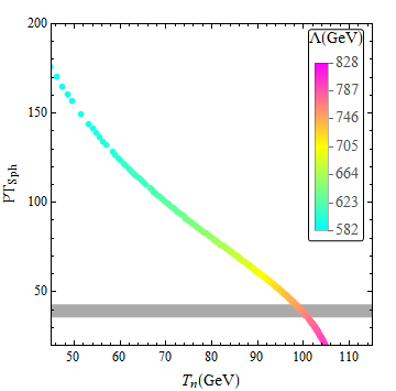
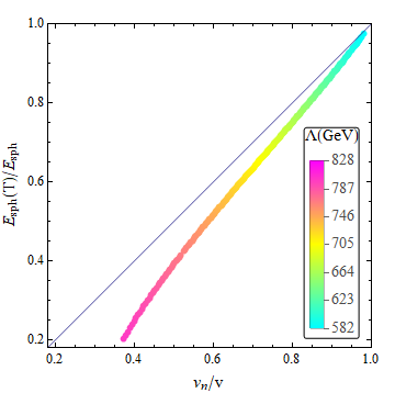
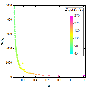
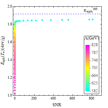
Figure 1: In the top panels, we plot $PT_{sph}$ versus $T_{n}$(left), and $E_{sph}(T_{n})/E_{sph}$ versus $v_{n}/v$(right) when varying $\Lambda$ for the case of the SMEFT. The bottom panels show $\beta/H_{n}$ versus $\alpha$ by color-coding $E_{sph}(T_{n})/T_{n}$(left), and the relation between the sphaleron energy $E_{sph}(T_{n})$ and the SNR of the GW spectra(right).

In the top panel of Fig. 1, we first present the relation between the BNPC and the new physics scale, where the horizontal shaded region represents the uncertainty of $\kappa$ in the sphaleron rate, i.e. the range $[35.9,42.8]$ in Eq.1 (this corresponds to $749<\Lambda<768$ GeV). When $PT_{sph}$ is above this region, the BNPC is satisfied, while $v_{n}/T_{n}\geq 1$ is obtained when $\Lambda<790$ GeV. The top-right panel demonstrates the scaling law, where the deviation from the scaling law becomes smaller when the phase transition strength becomes larger obtained with a lower new physics scale $\Lambda$. We further present the relation between $E_{sph}(T_{n})/T_{n}$ and the gravitational wave parameters $\alpha$ and $\beta/H_{n}$ in the bottom left panel. This demonstrates that a larger $\alpha$ (with a larger phase transition strength $v_{n}/T_{n}$) and a smaller $\beta/H_{n}$ generally lead to a larger $E_{sph}(T_{n})/T_{n}$, for which the sphaleron rate is highly suppressed and washout of the baryon asymmetry can be avoided. This correlation among these parameters is anticipated, as a larger $v_{n}$ can generally be obtained with a more significant supercooling. The relation between the sphaleron energy and the SNR of the corresponding gravitational wave spectra from the EWPT is shown in the bottom-right plot, which indicates that the sphaleron can be probed by the gravitational wave detector (with a larger SNR) when $\Lambda$ is lower. The $E_{sph}(T_{n})/T_{n}$ obtained for all EWPT points are smaller than the SM sphaleron energy at zero temperature.

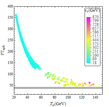
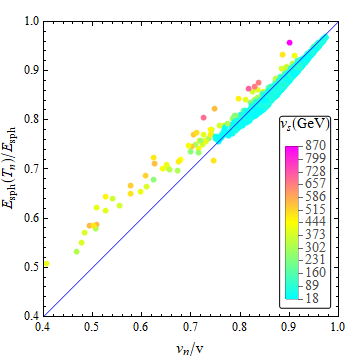
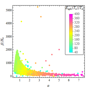
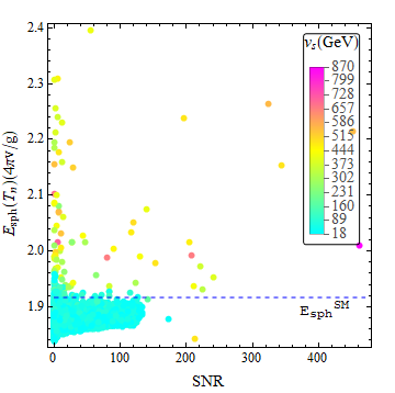
Figure 2: As in Fig. 1, we show similar plots with $v_{n}/T_{n}>1$ and SNR$>$10, where $v_{s}$ is the VEV of the singlet at zero temperature.

Now we move to another scenario, where the new physics that is necessary for a first order EWPT cannot be integrated out. We illustrate the situation with the xSM (see Ref.Damgaard:2015con ; Huang:2015tdv for the mismatch between the SMEFT and xSM model), and show in Fig.2 the points with SNR$>$10. The top-left panel of Fig.2 shows that a lower $v_{s}$ generally leads to a lower $T_{n}$ and a larger $PT_{sph}$. The top-right panel shows that the scaling law is better satisfied for small $v_{s}$. We then examine the relation between $E_{sph}(T_{n})/T_{n}$ and ($\alpha$, $\beta/H_{n}$) in the bottom-left panel, which indicates a similar behavior as the SMEFT case. The bottom-right panel shows that the sphaleron energy is concentrated at around 1.9 (in unit of $4\pi v/g$) for small $v_{s}$, where the GW signal can be probed by LISA Caprini:2015zlo . In the SNR calculation for the SFOEWPT points, we include the deficit found in the GW production from the sound waves Cutting:2019zws . The $E_{sph}(T_{n})/T_{n}$ for most SFOEWPT points are found to be smaller than the SM sphaleron energy at zero temperature.

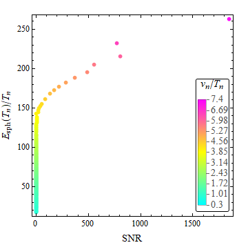
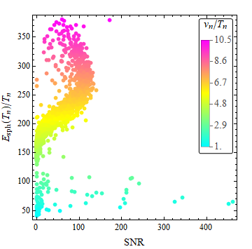
Figure 3: We show the SNR of the GW spectra versus the $E_{sph}/T_{n}$ by color-coding $v_{n}/T_{n}$ for SMEFT (left panel) and xSM (right panel).

We finally present Fig. 3, which shows that a EWPT which is strong enough to produce an observable gravitational wave signal can effectively “switch off” the sphaleron rate after the transition as required by the EWBG.

IV Conclusions and discussion

We have calculated the energy of the electroweak sphaleron during the EWPT and revealed the relation between the BNPC and the new physics scale using the SMEFT and xSM as two concrete examples. The scaling law can be established approximately when there is a higher phase transition strength associated with a lower new physics scale. In this scenario, it is possible to use the GW detectors to access the sphaleron energy, thus providing an alternative way of probing the sphaleron in addition to the high energy colliders. Different from other sources of the gravitational waves such as cosmic strings, domain walls, and primordial black hole, the GWs from SFOEWPT can also be tested through future colliders, since the SFOEWPT usually is accompanied by a deviation of the triple and quartic Higgs couplings in the Higgs potential . Thus the relation between the sphaleron energy and the phase transition strength studied here makes it possible to probe the sphaleron through both gravitational wave and collider measurements, in a complementary role.

At last, we note that our findings in this work rely only mildly on the numerical uncertainty in Eq. 1. Settling down the numerical range for a specific particle physics model would require a lattice simulation of the sphaleron rate Moore:1998swa .

Appendix A The GW Energy Density Spectra

It is realized in recent years that the long lasting sound waves in the plasma during and after the phase transition constitutes the dominant GW source Hindmarsh:2013xza ; Hindmarsh:2015qta . The energy density spectrum from this source is obtained by large scale numerical simulations, based on the scalar field and fluid model, for weak phase transitions corresponding to small values of $v_{w}$ and $\alpha$. It is well fitted by Hindmarsh:2015qta

$$\Omega_{\textrm{sw}}h^{2}=2.65\times 10^{-6}\left(\frac{H_{\ast}}{\beta}\right)\left(\frac{\kappa_{v}\alpha}{1+\alpha}\right)^{2}$$

$$\left(\frac{100}{g_{\ast}}\right)^{1/3}v_{w}\left(\frac{f}{f_{\text{sw}}}\right)^{3}\left(\frac{7}{4+3(f/f_{\textrm{sw}})^{2}}\right)^{7/2}\ ,$$ (15)

where $H_{\ast}$ is the Hubble rate at $T_{\ast}$ when the phase transition finished, which is only slightly different from $T_{n}$; $v_{w}$ is the bubble wall velocity and is chosen so that a non-relativistic relative velocity in the bubble wall frame can be obtained to make sure the slower baryon generation process is feasible No:2011fi ; Alves:2018jsw ; Alves:2019igs ; $g_{\ast}$ is the relativistic degrees of freedom. The factor $\kappa_{v}$ denotes the fraction of released energy density that is transferred into the kinetic energy of the plasma, which can be calculated given inputs of $v_{w}$ and $\alpha$ from a hydrodynamic analysis Espinosa:2010hh . Moreover $f_{\text{sw}}$ is the peak frequency:

$$f_{\textrm{sw}}=1.9\times 10^{-5}\frac{1}{v_{w}}\left(\frac{\beta}{H_{\ast}}\right)\left(\frac{T_{\ast}}{100\textrm{GeV}}\right)\left(\frac{g_{\ast}}{100}\right)^{1/6}\textrm{Hz}.$$ (16)

We note that the above formulae is limited to relatively small values of $v_{w}$ and $\alpha$. Recent numerical simulations exploring larger values of $\alpha$ shows a deficit in the GW production Cutting:2019zws (see Alves:2019igs for a more detailed discussion on the implications of this effect).

There is also a small fraction of energy going to the MHD, with a result that can be fitted by Caprini:2009yp ; Binetruy:2012ze

$$\Omega_{\textrm{turb}}h^{2}=3.35\times 10^{-4}\left(\frac{H_{\ast}}{\beta}\right)\left(\frac{\kappa_{\text{turb}}\alpha}{1+\alpha}\right)^{3/2}$$

$$\left(\frac{100}{g_{\ast}}\right)^{1/3}v_{w}\frac{(f/f_{\textrm{turb}})^{3}}{[1+(f/f_{\textrm{turb}})]^{11/3}(1+8\pi f/h_{\ast})}\;,\quad$$ (17)

where $\kappa_{\text{turb}}$ is the fraction of the energy transferred to the MHD turbulence and is approximately given by $\kappa_{\text{turb}}\approx(0.05\sim 0.1)\kappa_{v}$. We take here $\epsilon\approx 0.1$. Finally $f_{\text{turb}}$ is the peak frequency this spectrum:

$$f_{\textrm{turb}}=2.7\times 10^{-5}\frac{1}{v_{w}}\left(\frac{\beta}{H_{\ast}}\right)\left(\frac{T_{\ast}}{100\textrm{GeV}}\right)\left(\frac{g_{\ast}}{100}\right)^{1/6}\textrm{Hz}.$$ (18)

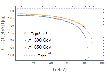
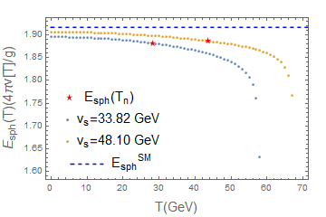
Figure 4: Left: $E_{sph}(T_{n})$ versus $T$ for the SMEFT, SNR$=175(0.002)$ and $v_{n}/T_{n}=4.8(2.6)$ for $\Lambda=590(650)$ GeV;Right: xSM scenario for $v_{s}=33.82(48.10)$ GeV, with $v_{n}/T_{n}=8.3(5.1)$ and $SNR=98(11)$.

Appendix B Sphaleron configurations

For the xSM model, we consider the following sphaleron field ansatz Fuyuto:2014yia :

$$A_{i}(\mu,r,\theta,\phi) =-\frac{i}{g}f(r)\partial_{i}U(\mu,\theta,\phi)U^{-1}(\mu,\theta,\phi),$$ (19)

$$H(\mu,r,\theta,\phi) =\frac{v(T)}{\sqrt{2}}\bigg{[}(1-h(r))\bigg{(}\begin{array}[]{c}0\\ e^{-i\mu}\cos\mu\end{array}\bigg{)}$$ (22)

$$+h(r)U(\mu,\theta,\phi)\bigg{(}\begin{array}[]{c}0\\ 1\end{array}\bigg{)}\bigg{]},$$ (25)

$$S(\mu,r,\theta,\phi) =v_{S}(T)k(r),$$ (26)

where $A_{i}$ are SU(2) gauge fields, and the matrix $U$ is defined as

$$U(\mu,\theta,\phi)=$$

$$\bigg{(}\begin{array}[]{cc}e^{i\mu}(c_{\mu}-is_{\mu}c_{\theta})&e^{i\phi}s_{\mu}s_{\theta}\\ -e^{-i\phi}s_{\mu}s_{\theta}&e^{-i\mu}(c_{\mu}+is_{\mu}c_{\theta})\end{array}\bigg{)},$$ (29)

where the $s_{\mu(\theta)}=\sin\mu(\theta)$ and $c_{\mu(\theta)}=\cos\mu(\theta)$. The sphaleron energy is obtained for $\mu=\pi/2$ Klinkhamer:1984di . From Eq. (II.3), the equations of motion can be found:

$$\frac{d^{2}f}{d\xi^{2}}=\frac{2}{\xi^{2}}f(1-f)(1-2f)-\frac{v[T]^{2}h^{2}}{4\Omega[T]^{2}}(1-f),$$ (30)

$$\frac{d}{d\xi}\left(\xi^{2}\frac{dh}{d\xi}\right)=2h(1-f)^{2}+\frac{\xi^{2}}{g^{2}}\frac{1}{v[T]^{2}\Omega[T]^{2}}\frac{\partial V_{\rm eff}(h,k,T)}{\partial h},$$ (31)

$$\frac{d}{d\xi}\left(\xi^{2}\frac{dk}{d\xi}\right)=\frac{\xi^{2}}{g^{2}}\frac{1}{v_{S}[T]^{2}\Omega[T]^{2}}\frac{\partial V_{\rm eff}(h,k,T)}{\partial k}.$$ (32)

The sphaleron solutions can be obtained with the following boundary conditions,

$$\lim_{\xi\to 0}f(\xi)=0,\lim_{\xi\to 0}h(\xi)=0,\quad\lim_{\xi\to 0}k^{\prime}(\xi)=0,$$

$$\lim_{\xi\to\infty}f(\xi)=1,\lim_{\xi\to\infty}h(\xi)=1,\lim_{\xi\to\infty}k(\xi)=1.$$ (33)

For the SMEFT, the sphaleron solutions can be obtained from:

$$\frac{d^{2}f}{d\xi^{2}}=\frac{2}{\xi^{2}}f(1-f)(1-2f)-\frac{1}{4}h^{2}(1-f),$$

$$\frac{d}{d\xi}\left(\xi^{2}\frac{dh}{d\xi}\right)=2h(1-f)^{2}+\frac{\xi^{2}}{g^{2}}\frac{1}{v[T]^{4}}\frac{\partial V_{\rm eff}(h,T)}{\partial h},\;$$ (34)

with boundary conditions given by,

$$\lim_{\xi\to 0}f(\xi)=0,\quad\ \lim_{\xi\to 0}h(\xi)=0,$$

$$\lim_{\xi\to\infty}f(\xi)=1,\quad\lim_{\xi\to\infty}h(\xi)=1\;.$$ (35)

We implement the relaxation method as documented in Numerical Recipes Press:2007:NRE:1403886 to solve the above ordinary differential equations numerically.

Here we present Fig. 4 to illustrate that the sphaleron energy at the temperature of the phase transition approaches the corresponding value at the zero temperature when one has a lower $\Lambda$ for SMEFT (or $v_{s}$ in xSM scenario), accompanied with a higher value of the phase transition strength and a larger SNR of the GW spectra. The value $E_{sph}(T)$ grows as the temperature of the universe decreases, and thus we have a increasingly suppressed sphaleron rate inside the electroweak bubbles after the EWPT.

References

- (1) LIGO Scientific, Virgo Collaboration, B. P. Abbott et al., “Observation of Gravitational Waves from a Binary Black Hole Merger,” Phys. Rev. Lett. 116 no. 6, (2016) 061102, arXiv:1602.03837 [gr-qc].
- (2) eLISA Collaboration, P. A. Seoane et al., “The Gravitational Universe,” arXiv:1305.5720 [astro-ph.CO].
- (3) V. A. Kuzmin, V. A. Rubakov, and M. E. Shaposhnikov, “On the Anomalous Electroweak Baryon Number Nonconservation in the Early Universe,” Phys. Lett. 155B (1985) 36.
- (4) D. E. Morrissey and M. J. Ramsey-Musolf, “Electroweak baryogenesis,” New J. Phys. 14 (2012) 125003, arXiv:1206.2942 [hep-ph].
- (5) A. Mazumdar and G. White, “Review of cosmic phase transitions: their significance and experimental signatures,” Rept. Prog. Phys. 82 no. 7, (2019) 076901, arXiv:1811.01948 [hep-ph].
- (6) A. D. Sakharov, “Violation of CP Invariance, C asymmetry, and baryon asymmetry of the universe,” Pisma Zh. Eksp. Teor. Fiz. 5 (1967) 32–35. [Usp. Fiz. Nauk161,no.5,61(1991)].
- (7) N. S. Manton, “Topology in the Weinberg-Salam Theory,” Phys. Rev. D28 (1983) 2019.
- (8) F. R. Klinkhamer and N. S. Manton, “A Saddle Point Solution in the Weinberg-Salam Theory,” Phys. Rev. D30 (1984) 2212.
- (9) V. A. Rubakov and M. E. Shaposhnikov, “Electroweak baryon number nonconservation in the early universe and in high-energy collisions,” Usp. Fiz. Nauk 166 (1996) 493–537, arXiv:hep-ph/9603208 [hep-ph]. [Phys. Usp.39,461(1996)].
- (10) X. Gan, A. J. Long, and L.-T. Wang, “Electroweak sphaleron with dimension-six operators,” Phys. Rev. D96 no. 11, (2017) 115018, arXiv:1708.03061 [hep-ph].
- (11) M. D’Onofrio, K. Rummukainen, and A. Tranberg, “Sphaleron Rate in the Minimal Standard Model,” Phys. Rev. Lett. 113 no. 14, (2014) 141602, arXiv:1404.3565 [hep-ph].
- (12) M. Dine, P. Huet, and R. L. Singleton, Jr., “Baryogenesis at the electroweak scale,” Nucl. Phys. B375 (1992) 625–648.
- (13) M. Quiros, “Finite temperature field theory and phase transitions,” in Proceedings, Summer School in High-energy physics and cosmology: Trieste, Italy, June 29-July 17, 1998, pp. 187–259. 1999. arXiv:hep-ph/9901312 [hep-ph].
- (14) S. Braibant, Y. Brihaye, and J. Kunz, “Sphalerons at finite temperature,” Int. J. Mod. Phys. A8 (1993) 5563–5574, arXiv:hep-ph/9302314 [hep-ph].
- (15) Y. Brihaye and J. Kunz, “Electroweak bubbles and sphalerons,” Phys. Rev. D48 (1993) 3884–3890, arXiv:hep-ph/9304256 [hep-ph].
- (16) C. Grojean, G. Servant, and J. D. Wells, “First-order electroweak phase transition in the standard model with a low cutoff,” Phys. Rev. D71 (2005) 036001, arXiv:hep-ph/0407019 [hep-ph].
- (17) C. Delaunay, C. Grojean, and J. D. Wells, “Dynamics of Non-renormalizable Electroweak Symmetry Breaking,” JHEP 04 (2008) 029, arXiv:0711.2511 [hep-ph].
- (18) S. R. Coleman and E. J. Weinberg, “Radiative Corrections as the Origin of Spontaneous Symmetry Breaking,” Phys. Rev. D7 (1973) 1888–1910.
- (19) R. R. Parwani, “Resummation in a hot scalar field theory,” Phys. Rev. D45 (1992) 4695, arXiv:hep-ph/9204216 [hep-ph]. [Erratum: Phys. Rev.D48,5965(1993)].
- (20) D. J. Gross, R. D. Pisarski, and L. G. Yaffe, “QCD and Instantons at Finite Temperature,” Rev. Mod. Phys. 53 (1981) 43.
- (21) H. H. Patel and M. J. Ramsey-Musolf, “Baryon Washout, Electroweak Phase Transition, and Perturbation Theory,” JHEP 07 (2011) 029, arXiv:1101.4665 [hep-ph].
- (22) S. Profumo, M. J. Ramsey-Musolf, and G. Shaughnessy, “Singlet Higgs phenomenology and the electroweak phase transition,” JHEP 08 (2007) 010, arXiv:0705.2425 [hep-ph].
- (23) S. Profumo, M. J. Ramsey-Musolf, C. L. Wainwright, and P. Winslow, “Singlet-catalyzed electroweak phase transitions and precision Higgs boson studies,” Phys. Rev. D91 no. 3, (2015) 035018, arXiv:1407.5342 [hep-ph].
- (24) A. V. Kotwal, M. J. Ramsey-Musolf, J. M. No, and P. Winslow, “Singlet-catalyzed electroweak phase transitions in the 100 TeV frontier,” Phys. Rev. D94 no. 3, (2016) 035022, arXiv:1605.06123 [hep-ph].
- (25) T. Huang, J. M. No, L. Pernié, M. Ramsey-Musolf, A. Safonov, M. Spannowsky, and P. Winslow, “Resonant di-Higgs boson production in the channel: Probing the electroweak phase transition at the LHC,” Phys. Rev. D96 no. 3, (2017) 035007, arXiv:1701.04442 [hep-ph].
- (26) A. Alves, T. Ghosh, H.-K. Guo, and K. Sinha, “Resonant Di-Higgs Production at Gravitational Wave Benchmarks: A Collider Study using Machine Learning,” JHEP 12 (2018) 070, arXiv:1808.08974 [hep-ph].
- (27) P. Huang, A. Joglekar, B. Li, and C. E. M. Wagner, “Probing the Electroweak Phase Transition at the LHC,” Phys. Rev. D93 no. 5, (2016) 055049, arXiv:1512.00068 [hep-ph].
- (28) A. Alves, T. Ghosh, H.-K. Guo, K. Sinha, and D. Vagie, “Collider and Gravitational Wave Complementarity in Exploring the Singlet Extension of the Standard Model,” JHEP 04 (2019) 052, arXiv:1812.09333 [hep-ph].
- (29) C. Caprini et al., “Science with the space-based interferometer eLISA. II: Gravitational waves from cosmological phase transitions,” JCAP 1604 no. 04, (2016) 001, arXiv:1512.06239 [astro-ph.CO].
- (30) C. L. Wainwright, “CosmoTransitions: Computing Cosmological Phase Transition Temperatures and Bubble Profiles with Multiple Fields,” Comput. Phys. Commun. 183 (2012) 2006–2013, arXiv:1109.4189 [hep-ph].
- (31) M. Hindmarsh, S. J. Huber, K. Rummukainen, and D. J. Weir, “Gravitational waves from the sound of a first order phase transition,” Phys. Rev. Lett. 112 (2014) 041301, arXiv:1304.2433 [hep-ph].
- (32) M. Hindmarsh, S. J. Huber, K. Rummukainen, and D. J. Weir, “Numerical simulations of acoustically generated gravitational waves at a first order phase transition,” Phys. Rev. D92 no. 12, (2015) 123009, arXiv:1504.03291 [astro-ph.CO].
- (33) A. Kosowsky, M. S. Turner, and R. Watkins, “Gravitational radiation from colliding vacuum bubbles,” Phys. Rev. D45 (1992) 4514–4535.
- (34) A. Kosowsky, M. S. Turner, and R. Watkins, “Gravitational waves from first order cosmological phase transitions,” Phys. Rev. Lett. 69 (1992) 2026–2029.
- (35) A. Kosowsky and M. S. Turner, “Gravitational radiation from colliding vacuum bubbles: envelope approximation to many bubble collisions,” Phys. Rev. D47 (1993) 4372–4391, arXiv:astro-ph/9211004 [astro-ph].
- (36) S. J. Huber and T. Konstandin, “Gravitational Wave Production by Collisions: More Bubbles,” JCAP 0809 (2008) 022, arXiv:0806.1828 [hep-ph].
- (37) R. Jinno and M. Takimoto, “Gravitational waves from bubble collisions: An analytic derivation,” Phys. Rev. D95 no. 2, (2017) 024009, arXiv:1605.01403 [astro-ph.CO].
- (38) R. Jinno and M. Takimoto, “Gravitational waves from bubble dynamics: Beyond the Envelope,” JCAP 1901 (2019) 060, arXiv:1707.03111 [hep-ph].
- (39) D. Bodeker and G. D. Moore, “Can electroweak bubble walls run away?,” JCAP 0905 (2009) 009, arXiv:0903.4099 [hep-ph].
- (40) L. Bian, H.-K. Guo, Y. Wu, and R. Zhou, “Gravitational wave and Collider searches for the EWSB patterns,” arXiv:1906.11664 [hep-ph].
- (41) C. Grojean and G. Servant, “Gravitational Waves from Phase Transitions at the Electroweak Scale and Beyond,” Phys. Rev. D75 (2007) 043507, arXiv:hep-ph/0607107 [hep-ph].
- (42) F. R. Klinkhamer and R. Laterveer, “The Sphaleron at finite mixing angle,” Z. Phys. C53 (1992) 247–252.
- (43) B. Kleihaus, J. Kunz, and Y. Brihaye, “The Electroweak sphaleron at physical mixing angle,” Phys. Lett. B273 (1991) 100–104.
- (44) J. Kunz, B. Kleihaus, and Y. Brihaye, “Sphalerons at finite mixing angle,” Phys. Rev. D46 (1992) 3587–3600.
- (45) A. Ahriche, “What is the criterion for a strong first order electroweak phase transition in singlet models?,” Phys. Rev. D75 (2007) 083522, arXiv:hep-ph/0701192 [hep-ph].
- (46) P. H. Damgaard, A. Haarr, D. O’Connell, and A. Tranberg, “Effective Field Theory and Electroweak Baryogenesis in the Singlet-Extended Standard Model,” JHEP 02 (2016) 107, arXiv:1512.01963 [hep-ph].
- (47) D. Cutting, M. Hindmarsh, and D. J. Weir, “Vorticity, kinetic energy, and suppressed gravitational wave production in strong first order phase transitions,” arXiv:1906.00480 [hep-ph].
- (48) A. Alves, D. Gonçalves, T. Ghosh, H.-K. Guo, and K. Sinha, “Di-Higgs Production in the Channel and Gravitational Wave Complementarity,” arXiv:1909.05268 [hep-ph].
- (49) F. L. Bezrukov, D. Levkov, C. Rebbi, V. A. Rubakov, and P. Tinyakov, “Semiclassical study of baryon and lepton number violation in high-energy electroweak collisions,” Phys. Rev. D68 (2003) 036005, arXiv:hep-ph/0304180 [hep-ph].
- (50) F. L. Bezrukov, D. Levkov, C. Rebbi, V. A. Rubakov, and P. Tinyakov, “Suppression of baryon number violation in electroweak collisions: Numerical results,” Phys. Lett. B574 (2003) 75–81, arXiv:hep-ph/0305300 [hep-ph].
- (51) A. Ringwald, “Electroweak instantons / sphalerons at VLHC?,” Phys. Lett. B555 (2003) 227–237, arXiv:hep-ph/0212099 [hep-ph].
- (52) A. Ringwald, “An Upper bound on the total cross-section for electroweak baryon number violation,” JHEP 10 (2003) 008, arXiv:hep-ph/0307034 [hep-ph].
- (53) J. Ellis and K. Sakurai, “Search for Sphalerons in Proton-Proton Collisions,” JHEP 04 (2016) 086, arXiv:1601.03654 [hep-ph].
- (54) Y.-C. Qiu and S. H. H. Tye, “Role of Bloch Waves in baryon-number violating processes,” Phys. Rev. D100 no. 3, (2019) 033006, arXiv:1812.07181 [hep-ph].
- (55) S. H. H. Tye and S. S. C. Wong, “Baryon Number Violating Scatterings in Laboratories,” Phys. Rev. D96 no. 9, (2017) 093004, arXiv:1710.07223 [hep-ph].
- (56) J. Ellis, K. Sakurai, and M. Spannowsky, “Search for Sphalerons: IceCube vs. LHC,” JHEP 05 (2016) 085, arXiv:1603.06573 [hep-ph].
- (57) S. H. H. Tye and S. S. C. Wong, “Bloch Wave Function for the Periodic Sphaleron Potential and Unsuppressed Baryon and Lepton Number Violating Processes,” Phys. Rev. D92 no. 4, (2015) 045005, arXiv:1505.03690 [hep-th].
- (58) S. Di Vita, G. Durieux, C. Grojean, J. Gu, Z. Liu, G. Panico, M. Riembau, and T. Vantalon, “A global view on the Higgs self-coupling at lepton colliders,” JHEP 02 (2018) 178, arXiv:1711.03978 [hep-ph].
- (59) T. Liu, K.-F. Lyu, J. Ren, and H. X. Zhu, “Probing the quartic Higgs boson self-interaction,” Phys. Rev. D98 no. 9, (2018) 093004, arXiv:1803.04359 [hep-ph].
- (60) G. D. Moore, “Measuring the broken phase sphaleron rate nonperturbatively,” Phys. Rev. D59 (1999) 014503, arXiv:hep-ph/9805264 [hep-ph].
- (61) J. O. Andersen, T. Gorda, A. Helset, L. Niemi, T. V. I. Tenkanen, A. Tranberg, A. Vuorinen, and D. J. Weir, “Nonperturbative Analysis of the Electroweak Phase Transition in the Two Higgs Doublet Model,” Phys. Rev. Lett. 121 no. 19, (2018) 191802, arXiv:1711.09849 [hep-ph].
- (62) T. Gorda, A. Helset, L. Niemi, T. V. I. Tenkanen, and D. J. Weir, “Three-dimensional effective theories for the two Higgs doublet model at high temperature,” JHEP 02 (2019) 081, arXiv:1802.05056 [hep-ph].
- (63) K. Kainulainen, V. Keus, L. Niemi, K. Rummukainen, T. V. I. Tenkanen, and V. Vaskonen, “On the validity of perturbative studies of the electroweak phase transition in the Two Higgs Doublet model,” JHEP 06 (2019) 075, arXiv:1904.01329 [hep-ph].
- (64) K. Farakos, K. Kajantie, K. Rummukainen, and M. E. Shaposhnikov, “3-D physics and the electroweak phase transition: Perturbation theory,” Nucl. Phys. B425 (1994) 67–109, arXiv:hep-ph/9404201 [hep-ph].
- (65) K. Kajantie, M. Laine, K. Rummukainen, and M. E. Shaposhnikov, “Generic rules for high temperature dimensional reduction and their application to the standard model,” Nucl. Phys. B458 (1996) 90–136, arXiv:hep-ph/9508379 [hep-ph].
- (66) J. M. No, “Large Gravitational Wave Background Signals in Electroweak Baryogenesis Scenarios,” Phys. Rev. D84 (2011) 124025, arXiv:1103.2159 [hep-ph].
- (67) J. R. Espinosa, T. Konstandin, J. M. No, and G. Servant, “Energy Budget of Cosmological First-order Phase Transitions,” JCAP 1006 (2010) 028, arXiv:1004.4187 [hep-ph].
- (68) C. Caprini, R. Durrer, and G. Servant, “The stochastic gravitational wave background from turbulence and magnetic fields generated by a first-order phase transition,” JCAP 0912 (2009) 024, arXiv:0909.0622 [astro-ph.CO].
- (69) P. Binetruy, A. Bohe, C. Caprini, and J.-F. Dufaux, “Cosmological Backgrounds of Gravitational Waves and eLISA/NGO: Phase Transitions, Cosmic Strings and Other Sources,” JCAP 1206 (2012) 027, arXiv:1201.0983 [gr-qc].
- (70) K. Fuyuto and E. Senaha, “Improved sphaleron decoupling condition and the Higgs coupling constants in the real singlet-extended standard model,” Phys. Rev. D90 no. 1, (2014) 015015, arXiv:1406.0433 [hep-ph].
- (71) W. H. Press, S. A. Teukolsky, W. T. Vetterling, and B. P. Flannery, Numerical Recipes 3rd Edition: The Art of Scientific Computing. Cambridge University Press, New York, NY, USA, 3 ed., 2007.