Noisy Guesses

Abstract

We consider the problem of guessing a random, finite–alphabet, secret $n$–vector, where the guesses are transmitted via a noisy channel. We provide a single–letter formula for the best achievable exponential growth rate of the $\rho$–th moment of the number of guesses, as a function of $n$. This formula exhibits a fairly clear insight concerning the penalty due to the noise. We describe two different randomized schemes that achieve the optimal guessing exponent. One of them is fully universal in the sense of being independent of source (that governs the vector to be guessed), the channel (that corrupts the guesses), and the moment power $\rho$. Interestingly, it turns out that, in general, the optimal guessing exponent function exhibits a phase transition when it is examined either as a function of the channel parameters, or as a function of $\rho$: as long as the channel is not too distant (in a certain sense to be defined precisely) from the identity channel (i.e., the clean channel), or equivalently, as long $\rho$ is larger than a certain critical value, $\rho_{\mbox{\tiny c}}$, there is no penalty at all in the guessing exponent, compared to the case of noiseless guessing.

Index Terms: guessing exponent, randomized guessing, noisy channels, phase transitions.

1 Introduction

Consider the problem of guessing the realization of a finite–alphabet random vector $\mbox{\boldmath$X$}=(X_{1},\ldots,X_{n})$ using a series of yes/no questions of the form: “Is $\mbox{\boldmath$X$}=\mbox{\boldmath$x$}_{1}$?”, “Is $\mbox{\boldmath$X$}=\mbox{\boldmath$x$}$?”, and so on, until a positive response is received. Given a distribution on $X$, a commonly used performance metric for the guessing problem is the expected number of guessing trials required until $X$ is guessed correctly, or more generally, a general moment of this number.

The quest for guessing strategies designed in order to minimize the moments of the number of guesses has several motivations and applications in information theory and related areas. One of them, for example, is sequential decoding, as shown by Arikan [1], who based his work on the earlier work of Massey [3], and related the asymptotic exponent of the best achievable guessing moment to the Rényi entropy. More recent applications of the guessing problem focus on aspects of information security, in particular, brute–force attacks of guessing passwords or decrypting messages protected by random keys. For example, one may submit a sequence of guessing queries in attempt to crack passwords – see, e.g., [5, Introduction] (as well as [6] and other references therein) for a fairly comprehensive review on guessing and information security, as well as for some historical perspective of earlier research work on the problem of guessing in general, along with its large variety of forms and extensions.

In this paper, we consider the guessing problem where the guesser (henceforth, Bob) submits his guesses to the party that examines the guesses (henceforth, Alice) via a noisy discrete memoryless channel (DMC). In other words, the problem is informally defined as follows: Alice randomly draws an $n$–vector $Y$ from a discrete memoryless source (DMS) $P$ of a finite alphabet ${\cal Y}$. Bob submits a sequence of guesses, $\mbox{\boldmath$x$}_{i}\in{\cal X}^{n}$, $i=1,2,\ldots$, but each guess $\mbox{\boldmath$x$}_{i}$ is transmitted through a DMC $W$, defined by a matrix single–letter transition probabilities, $\{W(y|x),~{}x\in{\cal X},~{}y\in{\cal Y}\}$, before arriving to Alice. Let $\mbox{\boldmath$Y$}_{1},\mbox{\boldmath$Y$}_{2},\ldots$, $\mbox{\boldmath$Y$}_{i}\in{\cal Y}^{n}$, $i=1,2,\ldots$, be the corresponding noisy versions of the guesses. Alice checks the noisy guesses sequentially, and returns an affirmative feedback to Bob upon the first perfect match, $\mbox{\boldmath$Y$}_{i}=\mbox{\boldmath$Y$}$. The questions we are studying, in this paper, are similar to those that were studied in earlier works on the guessing problem, namely: (i) what is the minimum achievable asymptotic exponent of $\mbox{\boldmath$E$}\{G^{\rho}\}$ (i.e., the guessing exponent), where $G$ is the number of guesses until the first success, and $\rho$ is an arbitrary given positive real? In particular, what is the penalty caused by the channel noise in terms of the possible increase in the guessing exponent, compared to the noiseless case of [1]? (ii) how can one achieve this minimum guessing exponent?

Our main result is a single–letter formula of the best achievable guessing exponent, i.e., the exponential growth rate of the $\rho$–th moment of the number of guesses, as a function of $n$. In particular, we provide two equivalent expressions of the optimal guessing exponent. One of these expressions immediately suggests an optimal (randomized) guessing strategy. The other expression exhibits a fairly clear insight concerning the penalty due to the noise. We describe two different randomized schemes that achieve the optimal guessing exponent. One of them is fully universal in the sense of being independent of source $P$ (that governs the vector $Y$ to be guessed), the channel $W$ (that corrupts the guesses), and the power $\rho$. Obviously, the existence of a randomized guessing scheme that achieves the optimal guessing exponent implies (albeit, not constructively) the existence of a deterministic guessing scheme, exactly like in standard random coding arguments. Having said that, randomized schemes have some advantages, as was discussed in [5].

Interestingly, it turns out that, in general, the optimal guessing exponent function exhibits a phase transition when it is examined either as a function of the channel parameters, $\{W(y|x)\}$, or as a function of $\rho$: as long as the channel is not too distant (in a certain sense to be defined precisely in the sequel) from the identity channel (i.e., the clean channel), or equivalently, as long $\rho$ is larger than a certain critical value, $\rho_{\mbox{\tiny c}}$, there is no penalty whatsoever in the guessing exponent, compared to the case of noiseless guessing.

There are several motivations for studying this problem of noisy guesses.

1. Since Alice and Bob might be physically remote from each other, it is conceivable that the channel that links Bob to Alice would be noisy, and coding/decoding may not be an option in applications where Alice has no incentive to cooperate with Bob.

2. Alice may wish to apply a jammer as a mean of defense against a (detected) brute–force attack conducted by Bob.

3. We wish to explore aspects of robustness of the guessing performance to errors in the guessing mechanism.

4. We believe that the results are fairly interesting and some of them are even quite surprising, for example, the phase transitions, and the full universality of two of the proposed guessing schemes, in $P$, $W$ and $\rho$, as described in the previous paragraphs.

5. It enriches the variety of perspectives and the plethora of technical analysis tools used in the guessing problem. While the guessing problem, in its ordinary, noiseless form, has an intimate relationship to source coding, and hence can be solved on the basis of source coding results, this is no longer the case in the noisy setting. Indeed, as we shall see, the analysis techniques are very different from those of noiseless guessing [1].

The outline of the remaining part of this paper is as follows. In Section 2, we establish notation conventions. In Section 3, we formally define the problem and the objectives. In Section 4, we present our main results and discuss them. Finally, in Section 5, we prove our main theorem.

2 Notation Conventions

Throughout the paper, random variables will be denoted by capital letters, specific values they may take will be denoted by the corresponding lower case letters, and their alphabets will be denoted by calligraphic letters. Random vectors and their realizations will be denoted, respectively, by capital letters and the corresponding lower case letters, both in the bold face font. Their alphabets will be superscripted by their dimensions. For example, the random vector $\mbox{\boldmath$X$}=(X_{1},\ldots,X_{n})$, ($n$ – positive integer) may take a specific vector value $\mbox{\boldmath$x$}=(x_{1},\ldots,x_{n})$ in ${\cal X}^{n}$, the $n$–th order Cartesian power of ${\cal X}$, which is the alphabet of each component of this vector. Sources and channels will be denoted by the letters $P$, $Q$, $V$ and $W$, subscripted by the names of the relevant random variables/vectors and their conditionings, if applicable, following the standard notation conventions, e.g., $Q_{X}$, $P_{Y|X}$, and so on. When there is no room for ambiguity, these subscripts will be omitted. The probability of an event ${\cal E}$ will be denoted by $\mbox{Pr}\{{\cal E}\}$, and the expectation operator will be denoted by $\mbox{\boldmath$E$}\{\cdot\}$. The entropy of a random variable $X$ with a generic distribution $Q_{X}$ (or $Q$, for short) will be denoted by $H(Q)$ or $H(Q_{X})$, or $H_{Q}(X)$, and the Kullback–Leibler divergence between two distributions, $P$ and $Q$, on the same alphabet, will be denoted by $D(Q\|P)$. Likewise, for a pair of random variables $(X,Y)$, jointly distributed according to $Q$, $H_{Q}(X,Y)$, $H_{Q}(X|Y)$, $I_{Q}(X;Y)$ will denote the joint entropy, the condition entropy of $X$ given $Y$, and the mutual information between $X$ and $Y$, respectively. Similar notation conventions will apply to other information measures, including those that involve more than two random variables. The weighted divergence between two conditional distributions, $Q_{Y|X}$ and $P_{Y|X}$, with weighting $Q_{X}$, is defined as

$$D(Q_{Y|X}\|P_{Y|X}|Q_{X})=\sum_{x\in{\cal X}}Q_{X}(x)\sum_{y\in{\cal Y}}Q_{Y|X}(y|x)\ln\frac{Q_{Y|X}(y|x)}{P_{Y|X}(y|x)}.$$ (1)

For two positive sequences $a_{n}$ and $b_{n}$, the notation $a_{n}\stackrel{{\scriptstyle\cdot}}{{=}}b_{n}$ will stand for equality in the exponential scale, that is, $\lim_{n\to\infty}\frac{1}{n}\log\frac{a_{n}}{b_{n}}=0$. Similarly, $a_{n}\stackrel{{\scriptstyle\cdot}}{{\leq}}b_{n}$ means that $\limsup_{n\to\infty}\frac{1}{n}\log\frac{a_{n}}{b_{n}}\leq 0$, and so on. The indicator function of an event ${\cal E}$ will be denoted by ${\cal I}\{E\}$. The notation $[x]_{+}$ will stand for $\max\{0,x\}$.

The empirical distribution of a sequence $\mbox{\boldmath$x$}\in{\cal X}^{n}$, which will be denoted by $\hat{P}_{\mbox{\boldmath$x$}}$, is the vector of relative frequencies $\hat{P}_{\mbox{\boldmath$x$}}(x)$ of each symbol $x\in{\cal X}$ in $x$. The type class of $\mbox{\boldmath$x$}\in{\cal X}^{n}$, denoted ${\cal T}(\mbox{\boldmath$x$})$, is the set of all vectors $\mbox{\boldmath$x$}^{\prime}$ with $\hat{P}_{\mbox{\boldmath$x$}^{\prime}}=\hat{P}_{\mbox{\boldmath$x$}}$. When we wish to emphasize the dependence of the type class on a generic empirical distribution, say, $Q_{X}$, we will denote it by ${\cal T}(Q_{X})$. Information measures associated with empirical distributions will be denoted with ‘hats’ and will be subscripted by the sequences from which they are induced. For example, the entropy associated with $\hat{P}_{\mbox{\boldmath$x$}}$, which is the empirical entropy of $x$, will be denoted by $\hat{H}_{\mbox{\boldmath$x$}}(X)$. An alternative notation, following the conventions described in the previous paragraph, is $H(\hat{P}_{\mbox{\boldmath$x$}})$. Similar conventions will apply to the joint empirical distribution, the joint type class, the conditional empirical distributions and the conditional type classes associated with pairs (and multiples) of sequences of length $n$. The conditional type class of $x$ given $y$ w.r.t. a conditional distribution $Q_{X|Y}$ will be denoted by ${\cal T}(Q_{X|Y}|\mbox{\boldmath$y$})$. $\hat{H}_{\mbox{\boldmath$x$}\mbox{\boldmath$y$}}(X,Y)$ will designate the empirical joint entropy of $x$ and $y$, $\hat{H}_{\mbox{\boldmath$x$}\mbox{\boldmath$y$}}(X|Y)$ will be the empirical conditional entropy, $\hat{I}_{\mbox{\boldmath$x$}\mbox{\boldmath$y$}}(X;Y)$ will denote empirical mutual information, and so on. Also, sometimes we will use the subscript $Q$ (like in $H_{Q}(X|Y)$ and $I_{Q}(X;Y)$) when it is understood that $Q$ is the joint empirical distribution associated with $(\mbox{\boldmath$x$},\mbox{\boldmath$y$})$.

3 Problem Formulation

We consider the following scenario: Alice draws a random $n$–vector, $\mbox{\boldmath$Y$}=(Y_{1},\ldots,Y_{n})$, from a discrete memoryless source (DMS), $P$, of a finite alphabet, ${\cal Y}$. Bob, who is unaware of the realization of $Y$, sequentially submits to Alice a (possibly, infinite) sequence of guesses, $\mbox{\boldmath$x$}_{1},\mbox{\boldmath$x$}_{2},\ldots$, where each $\mbox{\boldmath$x$}_{i}$ is a vector of length $n$, whose components take on values in a finite alphabet, ${\cal X}$. Before arriving to Alice, each guess, $\mbox{\boldmath$x$}_{i}$, undergoes a discrete memoryless channel (DMC), defined by a matrix of single–letter input–output transition probabilities, $W=\{W(y|x),~{}x\in{\cal X},~{}y\in{\cal Y}\}$. Let $\mbox{\boldmath$Y$}_{1},\mbox{\boldmath$Y$}_{2},\ldots$ be the corresponding noisy versions of $\mbox{\boldmath$x$}_{1},\mbox{\boldmath$x$}_{2},\ldots$, after being corrupted by the DMC, $W$. Alice sequentially examines the noisy guesses and she returns to Bob an affirmative feedback upon the first perfect match, $\mbox{\boldmath$Y$}_{i}=\mbox{\boldmath$Y$}$. Clearly, the number of guesses, $G$, until the first successful guess, is a random variable that depends on the source vector $Y$ and the guesses, $\mbox{\boldmath$Y$}_{1},\mbox{\boldmath$Y$}_{2},\ldots.$. It is given by

$$G=G(\mbox{\boldmath$Y$},\mbox{\boldmath$Y$}_{1},\mbox{\boldmath$Y$}_{2},\ldots)=\sum_{k=1}^{\infty}k\cdot{\cal I}\{\mbox{\boldmath$Y$}_{k}=\mbox{\boldmath$Y$}\}\cdot\prod_{i=1}^{k-1}[1-{\cal I}\{\mbox{\boldmath$Y$}_{i}=\mbox{\boldmath$Y$}\}].$$ (2)

For a given list of guesses, ${\cal G}_{n}=\{\mbox{\boldmath$x$}_{1},\mbox{\boldmath$x$}_{2},\ldots\}$, $\mbox{\boldmath$x$}_{i}\in{\cal X}^{n}$, $i=1,2,\ldots$, the $\rho$–th moment of $G$ is given by

$$\mbox{\boldmath$E$}_{{\cal G}_{n}}\{G^{\rho}\}=\sum_{\mbox{\boldmath$y$}\in{\cal Y}^{n}}P(\mbox{\boldmath$y$})\cdot\sum_{k=1}^{\infty}k^{\rho}\cdot W(\mbox{\boldmath$y$}|\mbox{\boldmath$x$}_{k})\cdot\prod_{i=1}^{k-1}[1-W(\mbox{\boldmath$y$}|\mbox{\boldmath$x$}_{i})],$$ (3)

where

$$W(\mbox{\boldmath$y$}|\mbox{\boldmath$x$})=W(y_{1},\ldots,y_{n}|x_{1},\ldots,x_{n})=\prod_{t=1}^{n}W(y_{t}|x_{t}).$$ (4)

Randomized guessing lists (where the deterministic guesses, $\{\mbox{\boldmath$x$}_{i}\}$, are replaced by random ones, $\{\mbox{\boldmath$X$}_{i}\}$) are allowed as well. In this case, eq. (3) would include also an expectation w.r.t. the randomness of the guesses. For a given sequence of lists, ${\cal G}={\cal G}_{1},{\cal G}_{2},\ldots$, we define

$${\cal E}_{{\cal G}}^{-}(\rho) = \liminf_{n\to\infty}\frac{\ln\mbox{\boldmath$E$}_{{\cal G}_{n}}\{G^{\rho}\}}{n}$$ (5)

$${\cal E}_{{\cal G}}^{+}(\rho) = \limsup_{n\to\infty}\frac{\ln\mbox{\boldmath$E$}_{{\cal G}_{n}}\{G^{\rho}\}}{n},$$ (6)

and

$${\cal E}^{-}(\rho) = \inf_{{\cal G}}{\cal E}_{{\cal G}}^{-}(\rho)$$ (7)

$${\cal E}^{+}(\rho) = \inf_{{\cal G}}{\cal E}_{{\cal G}}^{+}(\rho).$$ (8)

Our objectives, in this paper, are as follows.

1. To show that ${\cal E}^{-}(\rho)={\cal E}^{+}(\rho)$. The distinction between these two functions will then disappear and both of them will be denoted by ${\cal E}(\rho)$.

2. To find a single–letter formula for ${\cal E}(\rho)$, which depends on the source $P$ and the channel $W$, in addition to the moment order, $\rho$. To characterize the loss in the guessing performance due to the noise (compared to the case of noiseless guessing).

3. To derive a (possibly randomized) guessing scheme that achieves ${\cal E}(\rho)$.

In fact, all three objectives will essentially be accomplished in a joint manner. We will define a certain single–letter function, $E(\rho)$, and show that ${\cal E}^{+}(\rho)\leq E(\rho)\leq{\cal E}^{-}(\rho)$, where the first inequality is the direct part and the second inequality is the converse part. Using the obvious fact that ${\cal E}^{+}(\rho)\geq{\cal E}^{-}(\rho)$ by their definitions, all inequalities are in fact, equalities.

A comment about the notation is in order. When we wish to emphasize the dependence of $E(\rho)$ on the channel $W$ as well, we may expand the notation to $E(\rho,W)$. The second argument, $W$, may also be replaced by a certain parameter that completely defines $W$, like the crossover probability $q$ in case of the binary symmetric channel (BSC).

4 Main Results

Let $P$, $W$, and $\rho\geq 0$ be given. To present the main result, we first need a few definitions. For two given distributions, $Q_{X}$ and $Q_{Y}$, defined on ${\cal X}$ and ${\cal Y}$, respectively, define

$$\Gamma(Q_{X},Q_{Y})=\inf\{D(\tilde{Q}_{Y|X}\|W|Q_{X}):~{}(Q_{X}\odot\tilde{Q}_{Y|X})_{Y}=Q_{Y}\},$$ (9)

where the notation $(Q_{X}\odot\tilde{Q}_{Y|X})_{Y}=Q_{Y}$ means that the $Y$–marginal induced by the given $Q_{X}$ and by $\tilde{Q}_{Y|X}$ is constrained to be the given $Q_{Y}$, i.e., $\sum_{x\in{\cal X}}Q_{X}(x)\tilde{Q}_{Y|X}(y|x)=Q_{Y}(y)$ for all $y\in{\cal Y}$. Next, define

$$\Gamma(Q_{Y})=\inf_{Q_{X}}\Gamma(Q_{X},Q_{Y})=\inf_{Q_{X|Y}}D(Q_{Y|X}\|W|Q_{X}).$$ (10)

Finally, we define

$$E(\rho)=\sup_{Q_{Y}}\bigg{\{}\rho[H(Q_{Y})+\Gamma(Q_{Y})]-D(Q_{Y}\|P)\bigg{\}}.$$ (11)

Theorem 1 below states that $E(\rho)$ is, in fact, a single–letter formula for both ${\cal E}^{+}(\rho)$ and ${\cal E}^{-}(\rho)$. It also provides an alternative, equivalent expression for $E(\rho)$, which is simpler to calculate in practice.

Theorem 1

Let $P$, $W$, and $\rho\geq 0$ be given and consider the problem setting defined in Section 3. Assume that $W$ is such that $W_{\max}=\max_{x,y}W(y|x)<1$. Then,

1. (Converse part): ${\cal E}^{-}(\rho)\geq E(\rho)$.

2. (Direct part): ${\cal E}^{+}(\rho)\leq E(\rho)$.

3. The function $E(\rho)$ can also be expressed as follows:

   $$E(\rho)=\ln\left(\inf_{V}\sum_{y\in{\cal Y}}\frac{P(y)}{\left[\sum_{x\in{\cal X}}V(x)W(y|x)\right]^{\rho}}\right),$$ (12)

   where the infimum w.r.t. $V$ is taken across the simplex of all probability distributions over ${\cal X}$, i.e., over all vectors of dimension $|{\cal X}|$ whose components are non–negative and sum to unity.

The proof appears in Section 5. The remaining part of this section is devoted to a discussion on Theorem 1.

1. The assumption $W_{\max}<1$. This technical regularity condition is needed for the proof of the converse part. At a first glance, it seems to be rather restrictive. A closer look, however, reveals that this restriction is not too severe. Suppose that this condition is violated, namely, there exist pairs $(x,y)$ with $W(y|x)=1$. Let ${\cal Y}^{\prime}={\cal Y}\cap\{y:~{}\max_{x}W(y|x)=1\}$. Now, for any type $Q_{Y}$ whose support is ${\cal Y}^{\prime}$, and for every $\mbox{\boldmath$y$}\in{\cal T}(Q_{Y})$, we can find $x$ such that $W(\mbox{\boldmath$y$}|\mbox{\boldmath$x$})=1$, and the problem of guessing within such a type boils down to the problem of noiseless guessing: whenever one wishes to guess a certain $y$, he or she should guess instead an $x$ for which $W(\mbox{\boldmath$y$}|\mbox{\boldmath$x$})=1$. For every $Q_{Y}$ whose support is not included in ${\cal Y}^{\prime}$, and every $\mbox{\boldmath$y$}\in{\cal T}(Q_{Y})$, there exists at least one letter $y_{i}$ for which $W\stackrel{{\scriptstyle\Delta}}{{=}}\max_{x}W(y_{i}|x)<1$ and hence $W(\mbox{\boldmath$y$}|\mbox{\boldmath$x$})=\prod_{i=1}^{n}W(y_{i}|x_{i})\leq W<1$, which is still acceptable for the derivation of the converse proof (with $W$ replacing $W_{\max}^{n}$).

2. The penalty due to the noise and phase transitions. As can be seen from the first expression of $E(\rho)$ (eq. (11)), the term $\Gamma(Q_{Y})$ expresses the unavoidable, minimum achievable penalty that Bob must suffer due to the noise. Interestingly, there might be situations, where there is no penalty at all as far as the guessing exponent is concerned. These situations can be identified even more easily from the second expression of $E(\rho)$. First, observe that in the noiseless case, where $W$ is the clean channel, eq. (12) boils down to $E(\rho)=\ln(\inf_{Q}\sum_{y}P(y)/[Q(y)]^{\rho})$ ($Q$ being a probability distribution over ${\cal Y}$), which is achieved by the distribution $Q^{*}(y)$ that is proportional to $[P(y)]^{1/(1+\rho)}$. Eq. (12) can be thought of as the same minimization problem, except that now $Q$ is constrained to lie in the convex hull of $\{W(\cdot|x),~{}x\in{\cal X}\}$. Generally speaking, good channels have a relatively large convex hull, whereas bad channels have a relatively small one. In the extreme case of the clean channel, this convex hull is the entire simplex of probability distributions over ${\cal Y}$. In the other extreme, where the channel is completely useless, all $\{W(\cdot|x),~{}x\in{\cal X}\}$ coincide with a single distribution over ${\cal Y}$. In this case, the convex hull of $W$ is a singleton. Returning to the case of a general channel, $W$, if the above–mentioned distribution $Q^{*}$ happens to lie within this convex hull, then no penalty is incurred in the guessing exponent. Interestingly, this implies that in general there might be a phase transition in the behavior of the guessing exponent as a function of the noise level, or as a function of $\rho$. For a given source $P$ and a given moment order $\rho$, consider a family of channels defined by a single parameter. For example, consider the binary case (${\cal X}={\cal Y}=\{0,1\}$), where the binary source is defined by the parameter $p=\mbox{Pr}\{X_{i}=1\}$ and the family of channels are the binary symmetric channels (BSCs) with a crossover parameter $q\in[0,0.5]$. Assume also that $\rho=1$. If we increase $q$ gradually from $0$ to $0.5$, we see that as long as $q<q_{\mbox{\tiny c}}\stackrel{{\scriptstyle\Delta}}{{=}}\sqrt{p}/(\sqrt{p}+\sqrt{1-p})$, the guessing exponent is the same as in the noiseless case, independently of $q$. However, as $q$ crosses the critical value $q_{c}$ the guessing exponent starts to grow with $q$. The graph of the guessing exponent, here denoted $E(\rho,q)$, is depicted in Fig. 1, for $p=0.25$ and $\rho=1$, where $q_{\mbox{\tiny c}}=0.366$. Likewise, it is possible to examine the behavior of the guessing exponent as a function of $\rho$ for fixed $q$. In the case of the BSC, the convex hull of $W$ is always a symmetric interval around $0.5$, i.e., the interval $[q,1-q]$. The optimal distribution $Q^{*}$, defined above is a binary distribution with probabilities, $p^{1/(1+\rho)}/[p^{1/(1+\rho)}+(1-p)^{1/(1+\rho)}]$ and $(1-p)^{1/(1+\rho)}/[p^{1/(1+\rho)}+(1-p)^{1/(1+\rho)}]$. As $\rho$ grows, this distribution approaches the symmetric distribution, $(0.5,0.5)$. Therefore, there is critical value of $\rho$ beyond which this distribution falls in the convex hull of $\{q,1-q\}$. This critical value is given by

$$\rho_{\mbox{\tiny c}}\stackrel{{\scriptstyle\Delta}}{{=}}\left[\frac{\ln[(1-p)/p]}{\ln[(1-q)/q]}-1\right]_{+}.$$

Fig. 2 depicts the guessing exponent as a function of $\rho$, with $p=0.25$ and $q=0.35$, where $\rho_{\mbox{\tiny c}}=0.7747$.

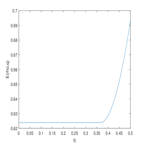
Figure 1: The function $E(\rho,q)$ vs. $q$ for the BSS with parameter $p=0.25$ and $\rho=1$. The critical value of $q$ is $q_{c}=\sqrt{p}/(\sqrt{p}+\sqrt{1-p})=0.366$.

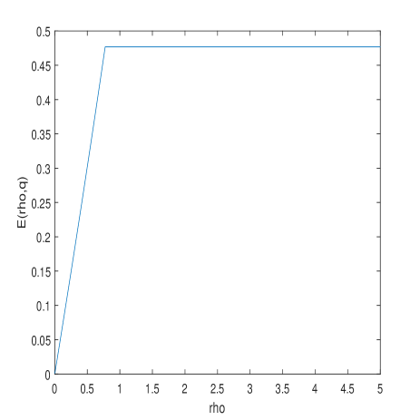
Figure 2: The function $E(\rho,q)$ vs. $\rho$ for the BSS with parameter $p=0.25$ and the BSC with parameter $q=0.35$. The critical value of $\rho$ is $\rho_{c}=\ln[(1-p)/p]/\ln[(1-q)/q]-1=0.7747$.

3. Operative significance of the alternative expression (12). Quite obviously, the alternative expression of $E(\rho)$, given in eq. (12), is easier to calculate in practice, than that of eq. (11). However, the advantage of (12) goes considerably beyond this point, as it has a simple operative interpretation. The denominator (without the power of $\rho$) is clearly the i.i.d. channel output distribution induced by an i.i.d. channel input distribution $V$ and the channel $W$. If we use randomized guessing and draw all our guesses according to the memoryless source $V(\mbox{\boldmath$x$})=\prod_{t=1}^{n}V(x_{t})$, then the noisy guesses will also be random guesses distributed according to $Q(\mbox{\boldmath$y$})=\prod_{t=1}^{n}Q(y_{t})$, where $Q(y)=\sum_{x}V(x)W(y|x)$. As is well known from previous work (see, e.g., [5], [6]), randomized guessing according to an i.i.d. distribution $Q$ yields a guessing exponent of $\ln(\sum_{y}P(y)/[Q(y)]^{\rho})$. But since $Q$ is constrained to have the form $Q(y)=\sum_{x}V(x)W(y|x)$, for a given $W$, the best one can do is to minimize this expression over $V$, which is exactly what eq. (12) tells us to do. It follows that the achievability of $E(\rho)$ is conceptually simple, thanks to eq. (12): find the channel input distribution $V^{*}$ that achieves the minimum in (12) and then generate random guesses according to $V^{*}(\mbox{\boldmath$x$})=\prod_{t=1}^{n}V^{*}(x_{t})$. It should be pointed out, however, that the optimal $V^{*}$ depends, in general, on $P$, $W$ and $\rho$, and therefore, this achievability scheme is not universal, as it requires the knowledge of these ingredients.

4. A universal guessing scheme. While $E(\rho)$ was argued in item 3 to be achievable by a non–universal guessing scheme, it turns out that $E(\rho)$ can also be achieved by a universal scheme that is independent of $P$, $W$ and $\rho$. Such a scheme is proposed in the direct part (part 2) of Theorem 1. This scheme is randomized: it is based on independent random selection of $\{\mbox{\boldmath$x$}_{i}\}$ according to the same universal distribution that was proposed in [5], namely,

$$P(\mbox{\boldmath$x$})=\frac{\exp\{-n\hat{H}_{\mbox{\boldmath$x$}}(X)\}}{\sum_{\tilde{\mbox{\boldmath$x$}}}\exp\{-n\hat{H}_{\tilde{\mbox{\boldmath$x$}}}(X)\}},$$ (13)

where $\hat{H}_{\mbox{\boldmath$x$}}(X)$ is the empirical entropy associated with $x$. The fact that this universal distribution continues to be asymptotically optimal even in the noisy case considered here, is not quite trivial, and it is even fairly surprising (at least to the author). It enhances even further the powerful properties of this distribution. We should mention also that random selection according to this distribution can be implemented efficiently in practice, as was shown in [5].

5. Side information. Suppose that Bob is equipped with a side information sequence $z$ that is correlated with the sequence $y$ to be guessed. More precisely, we assume that the sequence pair $(\mbox{\boldmath$y$},\mbox{\boldmath$z$})$ is drawn from a pair of correlated memoryless sources, $P(\mbox{\boldmath$y$},\mbox{\boldmath$z$})=\prod_{t=1}^{n}P(y_{t},z_{t})$, but only $z$ is available to Bob. It turns out that our results extend straightforwardly to this setting. Conceptually, once we condition on the given $z$, we are essentially back to the same setting as before. Thus, everything should be first conditioned on the side information, and finally, one should take the expectation w.r.t. the side information. As a result, the expressions of $E(\rho)$ extend as follows:

$$E(\rho)=\sup_{Q_{YZ}}\{\rho[H_{Q}(Y|Z)+\Gamma(Q_{YZ})]-D(Q_{YZ}\|P)],$$ (14)

where

$$\Gamma(Q_{YZ})=\inf_{Q_{X|YZ}}D(Q_{Y|XZ}\|W|Q_{XZ}),$$ (15)

and

$$E(\rho)=\ln\left[\sum_{z}P(z)\min_{V}\sum_{y}\frac{P(y|z)}{\left[\sum_{x}V(x|z)W(y|x)\right]^{\rho}}\right].$$ (16)

The universal guessing distribution defined in item 4 would be replaced by

$$P(\mbox{\boldmath$x$}|\mbox{\boldmath$z$})=\frac{\exp\{-n\hat{H}_{\mbox{\boldmath$x$}\mbox{\boldmath$z$}}(X|Z)\}}{\sum_{\tilde{\mbox{\boldmath$x$}}}\exp\{-n\hat{H}_{\tilde{\mbox{\boldmath$x$}}\mbox{\boldmath$z$}}(X|Z)\}},$$ (17)

where $\hat{H}_{\mbox{\boldmath$x$}\mbox{\boldmath$z$}}(X|Z)$ is the empirical conditional entropy of $X$ given $Z$, induced by the pair $(\mbox{\boldmath$x$},\mbox{\boldmath$z$})$ (see also [5]).

6. Sources and channels with memory. Another possible extension of our results addresses sources and channels with memory. In particular, our setting can essentially be extended to a class of sources and channels that obey the following fading memory conditions for some $B\geq 0$ (see also [2] and [7]).

$$P\left\{|\ln P(y_{1},\ldots,y_{k}|y_{-\ell},\ldots,y_{0})-\ln P(y_{1},\ldots,y_{k})|\geq B\right\}=0~{}~{}~{}\forall k,\ell\in{\cal N}$$ (18)

and

$$W\bigg{\{}|\ln W(y_{1},\ldots,y_{k}|x_{-\ell},\ldots,x_{k},y_{-\ell},\ldots,y_{0})-$$

$$\ln W(y_{1},\ldots,y_{k}|x_{1},\ldots,x_{k})|\geq B\bigg{|}x_{-\ell},\ldots,x_{k}\bigg{\}}=0~{}~{}~{}\forall k,\ell\in{\cal N}$$ (19)

Such sources and channels (like Markov sources and channels under certain conditions) can be approximated by block–i.i.d. probability measures and then the same derivations as before apply w.r.t. the super-alphabets of blocks. While one cannot expect single–letter formulas in this case, the point is that the universal probability distribution that is associated with the empirical entropy associated with these blocks can be replaced (and slightly improved) by the universal probability distribution, $P(\mbox{\boldmath$x$})\propto 2^{-LZ(\mbox{\boldmath$x$})}$, where $LZ(\mbox{\boldmath$x$})$ is the length (in bits) of the compressed version of $x$ by the Lempel–Ziv (LZ78) algorithm [8], as was shown in [5]. Therefore, this universal distribution is asymptotically optimal in terms of the guessing exponent whenever the source and the channel have fading memory in the above defined sense.

5 Proof of Theorem 1

5.1 Proof of Part 1 – the Converse Part

We begin from a simple preparatory step: let ${\cal T}(Q_{Y})$ be a given type class of $y$–vectors, and let $\mbox{\boldmath$x$}\in{\cal T}(Q_{X})$ be given. Then,

$$W[{\cal T}(Q_{Y})|\mbox{\boldmath$x$}] = \sum_{\mbox{\boldmath$y$}\in{\cal T}(Q_{Y})}W(\mbox{\boldmath$y$}|\mbox{\boldmath$x$})$$ (20)

$$= \sum_{{\cal T}(Q_{Y|X}|\mbox{\boldmath$x$})\subseteq{\cal T}(Q_{Y})}|{\cal T}(Q_{Y|X}|\mbox{\boldmath$x$})|\cdot\exp\{-n[H_{Q}(Y|X)+D(Q_{Y|X}\|W|Q_{X})]\}$$

$$\stackrel{{\scriptstyle\cdot}}{{=}} \sum_{{\cal T}(Q_{Y|X}|\mbox{\boldmath$x$})\subseteq{\cal T}(Q_{Y})}\exp\{nH_{Q}(Y|X)\}\cdot\exp\{-n[H_{Q}(Y|X)+D(Q_{Y|X}\|W|Q_{X})]\}$$

$$\stackrel{{\scriptstyle\cdot}}{{=}} \exp\left\{-n\inf_{\{Q_{Y|X}:~{}(Q_{X}\odot Q_{Y|X})_{Y}=Q_{Y}\}}D(Q_{Y|X}\|W|Q_{X})\right\}$$

$$= \exp\{-n\Gamma(Q_{X},Q_{Y})\},$$

and so,

$$\max_{\mbox{\boldmath$x$}\in{\cal X}^{n}}W[{\cal T}(Q_{Y})|\mbox{\boldmath$x$}]\stackrel{{\scriptstyle\cdot}}{{=}}\exp\{-n\inf_{Q_{X}}\Gamma(Q_{X},Q_{Y})\}=\exp\{-n\Gamma(Q_{Y})\}.$$ (21)

Now, let $c>0$ be an arbitrary constant, independent of $n$ (say, $c=1$), and for a given $Q_{Y}$, define

$$k(Q_{Y})=\bigg{\lceil}\frac{c\cdot|{\cal T}(Q_{Y})|}{\max_{\mbox{\boldmath$x$}\in{\cal X}^{n}}W[{\cal T}(Q_{Y})|\mbox{\boldmath$x$}]}\bigg{\rceil}\stackrel{{\scriptstyle\cdot}}{{=}}\exp\{n[H_{Q}(Y)+\Gamma(Q_{Y})]\}.$$ (22)

We next derive a lower bound to $\mbox{\boldmath$E$}\{G^{\rho}|\mbox{\boldmath$Y$}\in{\cal T}(Q_{Y})\}$ for a given ${\cal T}(Q_{Y})$.

$$\mbox{\boldmath$E$}\{G^{\rho}|\mbox{\boldmath$Y$}\in{\cal T}(Q_{Y})\} \stackrel{{\scriptstyle\mbox{\tiny(a)}}}{{\geq}} [k(Q_{Y})]^{\rho}\cdot\mbox{Pr}\{G\geq k(Q_{Y})|\mbox{\boldmath$Y$}\in{\cal T}(Q_{Y})\}$$ (23)

$$= [k(Q_{Y})]^{\rho}\cdot\frac{1}{|{\cal T}(Q_{Y})|}\sum_{\mbox{\boldmath$y$}\in{\cal T}(Q_{Y})}\prod_{i=1}^{k(Q_{Y})}[1-W(\mbox{\boldmath$y$}|\mbox{\boldmath$x$}_{i})]$$

$$= [k(Q_{Y})]^{\rho}\cdot\frac{1}{|{\cal T}(Q_{Y})|}\sum_{\mbox{\boldmath$y$}\in{\cal T}(Q_{Y})}\exp\left\{\sum_{i=1}^{k(Q_{Y})}\ln[1-W(\mbox{\boldmath$y$}|\mbox{\boldmath$x$}_{i})]\right\}$$

$$\stackrel{{\scriptstyle\mbox{\tiny(b)}}}{{\geq}} [k(Q_{Y})]^{\rho}\frac{1}{|{\cal T}(Q_{Y})|}\sum_{\mbox{\boldmath$y$}\in{\cal T}(Q_{Y})}\exp\left\{-\sum_{i=1}^{k(Q_{Y})}\frac{W(\mbox{\boldmath$y$}|\mbox{\boldmath$x$}_{i})}{1-W(\mbox{\boldmath$y$}|\mbox{\boldmath$x$}_{i})}\right\}$$

$$\stackrel{{\scriptstyle\mbox{\tiny(c)}}}{{\geq}} [k(Q_{Y})]^{\rho}\cdot\frac{1}{|{\cal T}(Q_{Y})|}\sum_{\mbox{\boldmath$y$}\in{\cal T}(Q_{Y})}\exp\left\{-\frac{1}{1-W_{\max}^{n}}\cdot\sum_{i=1}^{k(Q_{Y})}W(\mbox{\boldmath$y$}|\mbox{\boldmath$x$}_{i})\right\}$$

$$\stackrel{{\scriptstyle\mbox{\tiny(d)}}}{{\geq}} [k(Q_{Y})]^{\rho}\exp\left\{-\frac{1}{1-W_{\max}^{n}}\cdot\frac{1}{|{\cal T}(Q_{Y})|}\sum_{i=1}^{k(Q_{Y})}\sum_{\mbox{\boldmath$y$}\in{\cal T}(Q_{Y})}W(\mbox{\boldmath$y$}|\mbox{\boldmath$x$}_{i})\right\}$$

$$= [k(Q_{Y})]^{\rho}\exp\left\{-\frac{1}{(1-W_{\max}^{n})|{\cal T}(Q_{Y})|}\sum_{i=1}^{k(Q_{Y})}W[{\cal T}(Q_{Y})|\mbox{\boldmath$x$}_{i}]\right\}$$

$$\geq [k(Q_{Y})]^{\rho}\exp\left\{-\frac{k(Q_{Y})}{(1-W_{\max}^{n})|{\cal T}(Q_{Y})|}\max_{\mbox{\boldmath$x$}\in{\cal X}^{n}}W[{\cal T}(Q_{Y})|\mbox{\boldmath$x$}]\right\}$$

$$\stackrel{{\scriptstyle\mbox{\tiny(e)}}}{{\geq}} [k(Q_{Y})]^{\rho}\exp\bigg{\{}-\frac{1}{(1-W_{\max}^{n})}\times$$

$$\left(\frac{c\cdot|{\cal T}(Q_{Y})|}{\max_{\mbox{\boldmath$x$}\in{\cal X}^{n}}W[{\cal T}(Q_{Y})|\mbox{\boldmath$x$}]}+1\right)\cdot\frac{\max_{\mbox{\boldmath$x$}\in{\cal X}^{n}}W[{\cal T}(Q_{Y})|\mbox{\boldmath$x$}]}{|{\cal T}(Q_{Y})|}\bigg{\}}$$

$$= [k(Q_{Y})]^{\rho}\exp\left\{-\frac{1}{1-W_{\max}^{n}}\cdot\left(c+\frac{\max_{\mbox{\boldmath$x$}\in{\cal X}^{n}}W[{\cal T}(Q_{Y})|\mbox{\boldmath$x$}]}{|{\cal T}(Q_{Y})|}\right)\right\}$$

$$\stackrel{{\scriptstyle\mbox{\tiny(f)}}}{{\geq}} [k(Q_{Y})]^{\rho}\exp\left\{-\frac{c+1}{1-W_{\max}^{n}}\right\}$$

$$\stackrel{{\scriptstyle\cdot}}{{=}} \exp\{n\rho[H_{Q}(Y)+\Gamma(Q_{Y})]\},$$

where (a) follows from Markov’s inequality, (b) stems from the chain

$$\ln(1-x)=-\ln\left(1+\frac{x}{1-x}\right)\geq-\frac{x}{1-x},~{}~{}~{}~{}~{}~{}x<1,$$

(c) is implied by the assumption that $W_{\max}=\max_{x,y}W(y|x)<1$, (d) is by Jensen’s inequality, applied to the exponential function $f(x)=e^{-x}$, (e) is by the definition of $k(Q_{Y})$, and (f) is because $\max_{\mbox{\boldmath$x$}\in{\cal X}^{n}}W[{\cal T}(Q_{Y})|\mbox{\boldmath$x$}]\leq 1$ and $|{\cal T}(Q_{Y})|\geq 1$ for any non–empty type class. Finally,

$$\mbox{\boldmath$E$}\{G^{\rho}\} = \sum_{Q_{Y}}P[{\cal T}(Q_{Y})]\cdot\mbox{\boldmath$E$}\{G^{\rho}|\mbox{\boldmath$Y$}\in{\cal T}(Q_{Y})\}$$ (24)

$$\stackrel{{\scriptstyle\cdot}}{{\geq}} \sum_{Q_{Y}}\exp\{-nD(Q_{Y}\|P)\}\cdot\exp\{n\rho[H_{Q}(Y)+\Gamma(Q_{Y})]\}$$

$$\stackrel{{\scriptstyle\cdot}}{{=}} \exp\{n\max_{Q_{Y}}(\rho[H_{Q}(Y)+\Gamma(Q_{Y}))-D(Q_{Y}\|P))\}$$

$$= e^{nE(\rho)}.$$

5.2 Proof of Part 2 – the Direct Part

Consider a sequence of randomized guesses, all drawn independently from the universal distribution,

$$P(\mbox{\boldmath$x$})=\frac{\exp\{-n\hat{H}_{\mbox{\boldmath$x$}}(X)\}}{\sum_{\mbox{\boldmath$x$}^{\prime}\in{\cal X}^{n}}\exp\{-n\hat{H}_{\mbox{\boldmath$x$}^{\prime}}(X)\}},$$ (25)

for all $\mbox{\boldmath$x$}\in{\cal X}^{n}$. This induces the following distribution on the $y$–vectors:

$$Q(\mbox{\boldmath$y$}) \stackrel{{\scriptstyle\cdot}}{{=}} \sum_{\mbox{\boldmath$x$}\in{\cal X}^{n}}\exp\{-n\hat{H}_{\mbox{\boldmath$x$}}(X)\}\cdot W(\mbox{\boldmath$y$}|\mbox{\boldmath$x$})$$ (26)

$$\stackrel{{\scriptstyle\cdot}}{{=}} \sum_{{\cal T}(Q_{X|Y}|\mbox{\boldmath$y$})}|{\cal T}(Q_{X|Y}|\mbox{\boldmath$y$})|\cdot\exp\{-n[H_{Q}(X)+H_{Q}(Y|X)+D(Q_{Y|X}\|W|Q_{X})]\}$$

$$\stackrel{{\scriptstyle\cdot}}{{=}} \max_{Q_{X|Y}}\exp\{n[H_{Q}(X|Y)-H_{Q}(X)+H_{Q}(Y|X)+D(Q_{Y|X}\|W|Q_{X})]\}$$

$$\stackrel{{\scriptstyle\cdot}}{{=}} \exp\{-nH_{Q}(Y)\}\cdot\max_{Q_{X|Y}}\exp\{-nD(Q_{Y|X}\|W|Q_{X})]\}$$

$$\stackrel{{\scriptstyle\cdot}}{{=}} \exp\{-n[H_{Q}(Y)+\Gamma(Q_{Y})]\}.$$

Owing to [5, Lemma 1] and [4], for any given $\mbox{\boldmath$y$}\in{\cal T}(Q_{Y})$, the $\rho$–th moment of the number of guesses w.r.t. the randomized guessing, would then be of the exponential order of $1/[Q(\mbox{\boldmath$y$})]^{\rho}\stackrel{{\scriptstyle\cdot}}{{=}}\exp\{n\rho[H_{Q}(Y)+\Gamma(Q_{Y})]\}$. Finally, upon averaging this quantity with weights $P[{\cal T}(Q_{Y})]\stackrel{{\scriptstyle\cdot}}{{=}}\exp\{-nD(Q_{Y}\|P)\}$, we clearly obtain an expression of the exponential order of $e^{nE(\rho)}$. This completes the proof of the direct part.

5.3 Proof of Part 3 – the Alternative Expression

Consider the following chain of equalities:

$$E(\rho) = \sup_{Q_{Y}}\inf_{Q_{X|Y}}\left[\rho H(Q_{Y})+\rho D(Q_{Y|X}\|W|Q_{X})-D(Q_{Y}\|P)\right]$$ (27)

$$= \sup_{Q_{Y}}\inf_{Q_{X|Y}}\bigg{[}-\rho\sum_{y}Q_{Y}(y)\ln Q_{Y}(y)+\rho\sum_{x,y}Q_{XY}(x,y)\ln\frac{Q_{Y|X}(y|x)}{W(y|x)}+$$

$$\sum_{y}Q_{Y}(y)\ln\frac{P(y)}{Q_{Y}(y)}\bigg{]}$$

$$= \sup_{Q_{Y}}\inf_{Q_{X|Y}}\bigg{[}-\rho\sum_{y}Q_{Y}(y)\ln Q_{Y}(y)+\rho\sum_{x,y}Q_{XY}(x,y)\ln\frac{Q_{Y}(y)Q_{X|Y}(x|y)}{W(y|x)Q_{X}(x)}+$$

$$\sum_{y}Q_{Y}(y)\ln\frac{P(y)}{Q_{Y}(y)}\bigg{]}$$

$$= \sup_{Q_{Y}}\inf_{Q_{X|Y}}\bigg{[}\rho\sum_{x,y}Q_{XY}(x,y)\ln\frac{Q_{X|Y}(x|y)}{W(y|x)Q_{X}(x)}+\sum_{y}Q_{Y}(y)\ln\frac{P(y)}{Q_{Y}(y)}\bigg{]}$$

$$= \sup_{Q_{Y}}\inf_{Q_{X|Y}}\inf_{V}\left[\rho\sum_{x,y}Q_{XY}(x,y)\ln\frac{Q_{X|Y}(x|y)}{W(y|x)V(x)}+\sum_{y}Q_{Y}(y)\ln\frac{P(y)}{Q_{Y}(y)}\right]$$

$$= \sup_{Q_{Y}}\inf_{V}\inf_{Q_{X|Y}}\left[\rho\sum_{x,y}Q_{XY}(x,y)\ln\frac{Q_{X|Y}(x|y)}{W(y|x)V(x)}+\sum_{y}Q_{Y}(y)\ln\frac{P(y)}{Q_{Y}(y)}\right]$$

$$= \sup_{Q_{Y}}\inf_{V}\left[-\rho\sum_{y}Q_{Y}(y)\ln\left(\sum_{x}V(x)W(y|x)\right)+\sum_{y}Q_{Y}(y)\ln\frac{P(y)}{Q_{Y}(y)}\right]$$

$$\stackrel{{\scriptstyle\mbox{\tiny(a)}}}{{=}} \inf_{V}\sup_{Q_{Y}}\left[-\rho\sum_{y}Q_{Y}(y)\ln\left(\sum_{x}V(x)W(y|x)\right)+\sum_{y}Q_{Y}(y)\ln\frac{P(y)}{Q_{Y}(y)}\right]$$

$$= \inf_{V}\ln\left(\sum_{y}\frac{P(y)}{\left[\sum_{x}V(x)W(y|x)\right]^{\rho}}\right)$$

$$= \ln\left(\inf_{V}\sum_{y}\frac{P(y)}{\left[\sum_{x}V(x)W(y|x)\right]^{\rho}}\right),$$

where the equality (a) is due to the convexity in $V$ and the concavity in $Q_{Y}$ of the objective function. This completes the proof of Theorem 1.

References

- [1] E. Arikan, “An inequality on guessing and its application to sequential decoding,” IEEE Trans. Inform. Theory, vol. IT–42, no. 1, pp. 99–105, January 1996.
- [2] E. Arikan and N. Merhav, “Guessing subject to distortion,” IEEE Trans. Inform. Theory, vol. 44, no. 3, pp. 1041–1056, May 1998.
- [3] J. L. Massey, “Guessing and entropy,” Proc. IEEE International Symposium on Information Theory (ISIT ’94), p. 204, 1994.
- [4] N. Merhav, “Guessing individual sequences: generating randomized guesses using finite–state machines,” https://arxiv.org/pdf/1906.10857.pdf (submitted for publication, June 2019).
- [5] N. Merhav and A. Cohen, “Universal randomized guessing with application to asynchronous decentralized brute–force attacks,” to appear in IEEE Trans. Inform. Theory.
- [6] S. Salamatian, W. Huleihel, A. Beirami, A. Cohen, and M. Médard, “Why botnets work: distributed brute–force attacks need no synchronization,” IEEE Trans. Inform. Forensics and Security, vol. 14, no. 9, pp. 2288–2299, September 2019.
- [7] J. Ziv, “On classification with empirically observed statistics and universal data compression,” IEEE Trans. Ibform. Theory, vol. 34 no. 2, pp. 278–286, March 1988.
- [8] J. Ziv and A. Lempel, “Compression of individual sequences via variable-rate coding,” IEEE Trans. Inform. Theory, vol. IT–24, no. 5, pp. 530–536, September 1978.