Error detection on quantum computers improves accuracy of chemical calculations

Abstract

A major milestone of quantum error correction is to achieve the fault-tolerance threshold beyond which quantum computers can be made arbitrarily accurate. This requires extraordinary resources and engineering efforts. We show that even without achieving full fault tolerance, quantum error detection is already useful on the current generation of quantum hardware. We demonstrate this experimentally by executing an end-to-end chemical calculation for the hydrogen molecule encoded in the [[4, 2, 2]] quantum error-detecting code. The encoded calculation with logical qubits significantly improves the accuracy of the molecular ground-state energy.

I Introduction

Quantum computing promises efficient methods for quantum-chemical calculations that can reach far beyond the abilities of classical computers [1]. Large-scale calculations will require an ability to detect and correct errors. However, near-term devices known as noisy intermediate-scale quantum (NISQ) computers [2] are not expected to be fully fault-tolerant. Despite this limitation, they can still be useful for solving certain problems in physics and chemistry. In particular, the variational quantum eigensolver (VQE) [3, 4] is an algorithm designed to work well on NISQ computers. It has been experimentally demonstrated that VQE is able to find the ground state as well as excited states of small quantum systems encountered in quantum chemistry and nuclear physics [3, 5, 6, 7, 8, 9, 10, 11, 12]. The performance of NISQ algorithms is currently limited by gate errors and device noise. Several novel error mitigation and suppression techniques have been developed to overcome the imperfections of real devices [13, 14, 15, 16, 17, 18, 19, 20, 21, 22, 23, 24].

Quantum error correction (QEC) [25, 26, 27, 28, 29] is a theory developed in the last two decades to address this problem in a systematic way. An important milestone for QEC experiments is to achieve the fault-tolerance threshold. Fault tolerance requires a large number of qubits, long coherence times, and low gate errors. However, QEC can still be useful even without achieving fault tolerance and even with only a small number of qubits [30, 31, 32]. QEC can potentially increase coherence times and reduce error rates in existing devices. There have been efforts to demonstrate that quantum circuits using QEC codes can improve accuracy, or at least break even, in comparison with the original circuits. Previous experiments studied quantum codes that encode a single logical qubit [33, 34] and also demonstrated necessary improvements in qubit and gate qualities for QEC [35, 36, 37]. There has also been a growing interest in studying the [[4, 2, 2]] quantum code [38, 39, 40, 41, 42]. Recently, it has been shown that logical gates encoded in this code can achieve better fidelities than corresponding physical gates [43]. These efforts have tested individual steps of QEC protocols separately. However, it has never been demonstrated that an encoded calculation provides a tangible benefit in practical applications.

In this work we demonstrate that QEC provides an improvement in accuracy in an end-to-end quantum-chemical calculation. We have implemented a two-qubit VQE algorithm for calculating the ground-state energy of the hydrogen dimer in the [[4, 2, 2]] QEC code [44, 45, 27]. Instead of two physical qubits, the calculation uses two logical qubits encoded in four physical qubits. The code facilitates detection of a single bit-flip and phase-flip error in either of the two logical qubits. Our circuit additionally uses two ancillary qubits to perform a syndrome measurement during the initial state preparation and to perform a logical qubit rotation. Analytical simulations predict that the encoded circuit should outperform the physical circuit up to a fairly large error rate. We implement both the two-qubit and the six-qubit circuit on the IBM Q Experience platform.

II Quantum algorithm

Finding the ground-state energy of the $\mathrm{H}_{2}$ molecule in the minimal basis is the simplest molecular electronic-structure problem. It is often used as a benchmark and allows us to evaluate our approach in comparison to earlier work [5, 6, 8, 10, 20, 11].

The $\mathrm{H}_{2}$ molecular Hamiltonian can be transformed into a qubit Hamiltonian using the Jordan–Wigner [46], Bravyi–Kitaev [47], or another similar transformation. Here we use the explicit transformation defined in Ref. [8] that maps the subspace of the Hamiltonian corresponding to two electrons with zero total spin to a two-qubit Hamiltonian. The transformed Hamiltonian is given by

$$H=g_{1}+g_{2}Z_{1}+g_{3}Z_{2}+g_{4}Z_{1}Z_{2}+g_{5}X_{1}X_{2},$$ (1)

where $X_{i}$, $Y_{i}$, and $Z_{i}$ denote Pauli operators acting on qubit $i$ and $g_{j}$ are classically-calculated coefficients that depend on the internuclear separation $R$. We use values of $g_{j}$ published in Ref. [8].

The VQE algorithm performs particularly well for this problem. It is a hybrid quantum-classical algorithm that uses a quantum computer to create and measure the properties of a parametrized trial wavefunction and a classical computer to optimize the wavefunction parameters. Our trial wavefunction is the unitary coupled-cluster (UCC) ansatz [48, 49]. Its realization on quantum computers in context of quantum chemistry has been studied in Ref.  [3, 5, 10] and in our case is given by

$$\lvert\psi(\theta)\rangle=e^{-i\theta Y_{1}X_{2}/2}\lvert\Phi\rangle,$$ (2)

where $\theta$ is a parameter and $\lvert\Phi\rangle=\lvert 00\rangle$ is the Hartree–Fock wavefunction. The ansatz energy is given by

$$E(\theta)=g_{1}+g_{2}\langle Z_{1}\rangle_{\theta}+g_{3}\langle Z_{2}\rangle_{\theta}+g_{4}\langle Z_{1}Z_{2}\rangle_{\theta}+g_{5}\langle X_{1}X_{2}\rangle_{\theta},$$ (3)

where $\langle O\rangle_{\theta}=\langle\psi(\theta)\rvert O\lvert\psi(\theta)\rangle$. VQE uses a quantum computer to estimate the expectation values included in $E(\theta)$ and a classical optimizer to find the value of $\theta$ that minimizes $E(\theta)$. Since our ansatz depends on a single parameter only, we sample the full domain of $\theta$ and use a peak-finding routine to minimize $E(\theta)$. It is then sufficient to sample the individual expectation values in Eq. (3) only once and use the same data with any set of coefficients $g_{j}$. A quantum circuit that implements VQE is shown in the top of Fig. 1.

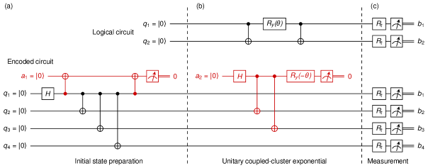
Figure 1: Quantum circuits for the preparation of the UCC ansatz and for the measurement of the expectation values in Eq. (3). The two-qubit logical circuit is shown above the corresponding six-qubit encoded circuit. Qubits $a_{1}$ and $a_{2}$ are ancillas. (a) The first section of the encoded circuit prepares the $\overline{\lvert 00\rangle}$ logical state. Ancilla $a_{1}$ is used to detect errors during the preparation. (b) The middle circuit sections apply the UCC exponential. We use ancilla $a_{2}$ to implement the rotation $\overline{R_{y}^{1}(\theta)}$. (c) The last circuit sections measure the expectation values. Gates $R_{t}$ perform a basis transformation that depends on the measured term.

III Error-detecting code

Our goal is to compare the performance of a circuit implemented with physical qubits to a circuit implemented with logical qubits of the [[4, 2, 2]] code. This code maps two logical qubits into a subspace of four physical qubits as

$$\overline{\lvert 00\rangle} =\frac{1}{\sqrt{2}}\left(\lvert 0000\rangle+\lvert 1111\rangle\right),$$ (4)

$$\overline{\lvert 01\rangle} =\frac{1}{\sqrt{2}}\left(\lvert 0011\rangle+\lvert 1100\rangle\right),$$

$$\overline{\lvert 10\rangle} =\frac{1}{\sqrt{2}}\left(\lvert 0101\rangle+\lvert 1010\rangle\right),$$

$$\overline{\lvert 11\rangle} =\frac{1}{\sqrt{2}}\left(\lvert 0110\rangle+\lvert 1001\rangle\right),$$

where an overline denotes a logical wavefunction. This mapping allows for the detection of one single-qubit error. To implement the circuit, we have to construct the required logical gates from the set of available physical gates. Our set of physical gates is limited to arbitrary single-qubit gates and $\mathit{CNOT}$ gates between any pairs of physical qubits.

The encoded circuit is shown in the bottom of Fig. 1. Its first part is a preparation of the initial logical state $\overline{\lvert 00\rangle}$. The circuit uses an ancilla measurement to detect an error during the preparation [30]. The measurement outcome zero corresponds to no error while the outcome one signals an error.

Some logical gates can be implemented easily because the corresponding physical gates act transversally, i.e., they can be implemented with only single-qubit physical gates. The [[4, 2, 2]] code also facilitates a very simple implementation of the logical $\mathit{CNOT}$ gates as $\overline{\mathit{CNOT}}_{12}=\mathit{SWAP}_{12}$ and $\overline{CNOT}_{21}=\mathit{SWAP}_{13}$, where an overline denotes a logical gate and $\mathit{SWAP}_{ij}$ swaps physical qubits $i$ and $j$ [43]. We implement $\mathit{SWAP}_{ij}$ and therefore the $\overline{\mathit{CNOT}}$ gates without performing any physical operation by relabelling the respective qubits.

The arbitrary-angle rotation of the first logical qubit $\overline{R_{y}^{1}(\theta)}$ cannot be implemented transversally. We apply this gate by entangling the logical qubit with an ancilla and performing a rotation and a measurement on the ancilla. The measurement projects the wavefunction onto a rotated logical state. The rotation circuit applies a $\theta$-rotation and a $-\theta$-rotation to the $\overline{\lvert 0\rangle}$ and $\overline{\lvert 1\rangle}$ states of the first logical qubit, respectively. The complete circuit performs a $\theta$-rotation because our logical wavefunction is initially prepared in the $\overline{\lvert 00\rangle}$ state. A general gate would require additional physical gates. Measured value zero in the ancilla corresponds to a rotation by $\theta$ while one corresponds to a rotation by $\theta+\pi$. We use both outcomes to sample the Hamiltonian terms.

Qubits are measured in the computational basis. Expectation value measurements require basis transformations that are performed with gates $R_{t}$. In particular, $R_{t}=I$ for the $\langle Z_{1}\rangle_{\theta}$, $\langle Z_{2}\rangle_{\theta}$, and $\langle Z_{1}Z_{2}\rangle_{\theta}$ terms as the respective operators are already diagonal in the computational basis, and $R_{t}=H$ for the $\langle X_{1}X_{2}\rangle_{\theta}$ term. We detect a single bit-flip or a single phase-flip error by calculating the parity of the measured code qubits.

Our encoded circuit is not fully fault-tolerant. In particular, not all single-qubit errors in logical rotation $\overline{R_{y}^{1}(\theta)}$ can be detected. We can also detect a bit-flip or a phase-flip, but not both at the same time (see Appendix E for details).

IV Experiment

The algorithm can be summarized as follows. We sample the $\langle Z_{1}\rangle_{\theta}$, $\langle Z_{2}\rangle_{\theta}$, $\langle Z_{1}Z_{2}\rangle_{\theta}$, and $\langle X_{1}X_{2}\rangle_{\theta}$ terms for $\theta\in[-\pi,\pi)$ on a quantum computer. The $\langle Z_{1}\rangle_{\theta}$, $\langle Z_{2}\rangle_{\theta}$, and $\langle Z_{1}Z_{2}\rangle_{\theta}$ terms are measured with a single circuit without any basis transformations. We execute the circuit with $R_{t}=H$ to measure the $\langle X_{1}X_{2}\rangle_{\theta}$ term. The ground-state energy for each internuclear separation $R$ is then calculated by minimizing $E(\theta)$. Unlike classical variational algorithms, the minimal energy can be lower than the exact energy due to systematic errors and noise.

We ran both the two-qubit logical circuit and the six-qubit encoded circuit on the Tokyo chip on IBM Q Experience. The major errors on this platform are readout errors [6, 9, 50]. If a qubit is in the $\lvert 0\rangle$ state, there is a significant probability of measuring outcome one and vice versa. The readout errors are asymmetric, i.e., the probability of measuring zero when a qubit state is $\lvert 1\rangle$ is higher than the probability of measuring one when the state is $\lvert 0\rangle$. This is mostly due to the readout time being significant in comparison to the $T_{1}$ coherence time, so the qubit can decay from the $\lvert 1\rangle$ state to the $\lvert 0\rangle$ state during the readout. We employed a readout error correction technique known as unfolding based on a Bayesian probabilistic model [51]. We first measured and estimated the probability of each outcome when the qubits were prepared in each computational basis state. We then used this probability matrix to iteratively unfold all measured counts to corresponding true counts (see Appendix C for details).

The chip contained 20 qubits arranged in a two-dimensional geometry. There were 72 ways to map our two-qubit physical circuit and 288 ways to map our six-qubit encoded circuit to the chip qubits. We found that the results depended significantly on the chosen qubits and also on the order of the applied gates. The result variability is illustrated in Fig. 2, where 2A and 2B denote two-qubit mappings $\left(q_{1},q_{2}\right)=\left(1,6\right)$ and $\left(q_{1},q_{2}\right)=\left(14,18\right)$, and 6A and 6B denote six-qubit mappings $\left(a_{1},a_{2},q_{1},q_{2},q_{3},q_{4}\right)=\left(13,9,8,4,3,12\right)$ and $\left(a_{1},a_{2},q_{1},q_{2},q_{3},q_{4}\right)=\left(5,15,11,16,10,17\right)$. The $\langle X_{1}X_{2}\rangle_{\theta}$ term is the most sensitive term in Eq. (3). To find an optimal mapping, we measured $\langle X_{1}X_{2}\rangle_{\theta}$ for $\theta=-3\pi/4$, $-\pi/2$, $-\pi/4$, $0$, $\pi/4$, $\pi/2$, and $3\pi/4$, applied readout error correction, and calculated the $L^{1}$ distances between the corrected results and the exact results for each mapping. We used the mappings with the smallest distances to run the final circuits. The compiler reordered gates based on the qubit mapping, so this technique took into account both the qubit mapping and the gate order variability.

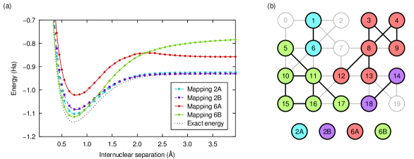
Figure 2: Variability of results with qubit mapping. (a) Examples of potential energy curves obtained using two random mappings for each circuit on the 20-qubit Tokyo chip. (b) Chip geometry with highlighted two-qubit mappings 2A and 2B, and six-qubit mappings 6A and 6B.

We executed the final calculations for both the two-qubit and the six-qubit circuit using the optimal mappings $\left(q_{1},q_{2}\right)=\left(13,18\right)$ for the two-qubit circuit and $\left(a_{1},a_{2},q_{1},q_{2},q_{3},q_{4}\right)=\left(12,5,11,6,10,17\right)$ for the six-qubit circuit. The $\langle Z_{1}\rangle_{\theta}$, $\langle Z_{2}\rangle_{\theta}$, $\langle Z_{1}Z_{2}\rangle_{\theta}$, and $\langle X_{1}X_{2}\rangle_{\theta}$ terms were obtained for 257 values of $\theta$ in the $[-\pi,\pi]$ interval. Each measured value was sampled with 8192 shots. For the encoded six-qubit circuit we postselected the outcomes based on their ancilla values. In particular, we measured all six qubits, performed readout error correction, and discarded outcomes with value one in the first ancilla and outcomes outside of the code space. Outcomes with values zero and one in the second ancilla were processed as samples corresponding to rotations by $\theta$ and $\theta\pm\pi$, respectively. We summed the renormalized counts of constituent basis states in Eq. (4) to calculate the logical state counts. The calculated expectation values of the Hamiltonian terms are shown in Fig. 3. We then used a peak-finding routine to find $\theta$ that minimized the energy in Eq. (3) for each internuclear separation. The calculated energy potential curves are shown in Fig. 4. The results demonstrate that the six-qubit encoded circuit improves the accuracy of the ground-state energy. The $\langle Z_{1}\rangle_{\theta}$ and $\langle Z_{2}\rangle_{\theta}$ terms contribute to $E(\theta)$ the most at small internuclear separations $R$ while the $\langle X_{1}X_{2}\rangle_{\theta}$ term is dominant at large $R$. The encoded circuit performs better especially at small $R$ where $\theta\approx 0$. Both energy potential curves are slightly inaccurate at large $R$. These inaccuracies can be fully explained by errors in $\langle X_{1}X_{2}\rangle_{\theta}$ at $\theta\approx-\pi/2$. The $\langle X_{1}X_{2}\rangle_{\theta}$ term is very sensitive to the quality of Hadamard gates applied before the measurement. Small inaccuracies lead to many nonvanishing coefficients in the final wavefunction. Our results suggest that the [[4, 2, 2]] code lacks the power to reliably detect errors in the $\langle X_{1}X_{2}\rangle_{\theta}$ term on this hardware (see Appendix E for details).

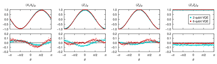
Figure 3: Measured expectation values of terms in the Hamiltonian for both the two-qubit and the six-qubit circuit. The top panels show the expectation values and the bottom panels show their differences from the exact values. The spread in values of neighboring points is due to shot noise.

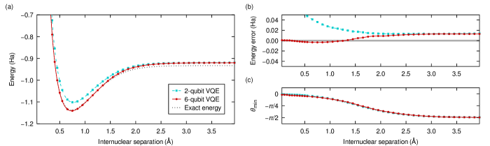
Figure 4: Comparison of VQE results obtained with the two-qubit and the six-qubit circuit using the best available qubits. (a) Energy potential curve of the $\mathrm{H}_{2}$ molecule. The exact energy is the lowest eigenvalue of Hamiltonian (1). (b) Difference between the measured energy and the exact energy. Gray band shows the range of chemical accuracy ($1.6\times 10^{-3}\,\mathrm{Ha}$). (c) Value of the UCC parameter $\theta$ at the energy minimum.

V Discussion

Our encoded circuit requires more physical qubits and gates than our logical circuit and is therefore more sensitive to errors. However, the gain by using the code was larger than the loss due to the circuit complexity. The results show that quantum error detection is already useful on NISQ devices even without achieving full fault tolerance. The presented method can be used in addition to other error mitigation techniques. Our implementation uses two ancillary qubits with postselection on their measured outcomes. In principle, it would be possible to use just one ancilla if we had an ability to perform a qubit reset. Similarly, the postselection in the rotation gate would be unnecessary if we had an ability to apply conditional gates dependent on measurement outcomes.

Some of the previous VQE experiments [5, 6, 8, 10, 20, 11] found the ground-state energy of the $\mathrm{H}_{2}$ molecule with a comparable or better accuracy. They used techniques like higher qubit states measurement [5], quantum subspace expansion [8], and noise extrapolation [20] to mitigate errors. We emphasize that our circuits do not use any such techniques. Our QEC method demonstrates that on the same hardware and using the same algorithm, the encoded circuit results in smaller errors than the physical circuit. Other error mitigation techniques are complementary to the presented method.

Appendix A Hamiltonian transformation

We use a transformation presented in Ref. [8] to map the electronic-structure space to qubits. The transformed space corresponds to a $\mathrm{H}_{2}$ molecule with two electrons and zero total spin. In particular,

$$a_{1\uparrow}^{\dagger}a_{1\downarrow}^{\dagger}\lvert\mathrm{vac}\rangle \to\lvert 00\rangle,$$ (5)

$$a_{1\uparrow}^{\dagger}a_{2\downarrow}^{\dagger}\lvert\mathrm{vac}\rangle \to\lvert 01\rangle,$$

$$a_{2\uparrow}^{\dagger}a_{1\downarrow}^{\dagger}\lvert\mathrm{vac}\rangle \to\lvert 10\rangle,$$

$$a_{2\uparrow}^{\dagger}a_{2\downarrow}^{\dagger}\lvert\mathrm{vac}\rangle \to\lvert 11\rangle,$$

where $a_{is}^{\dagger}$ is an operator that creates an electron with spin $s$ in orbital $i$ and $\lvert\mathrm{vac}\rangle$ is the vacuum state.

Appendix B Analytical model

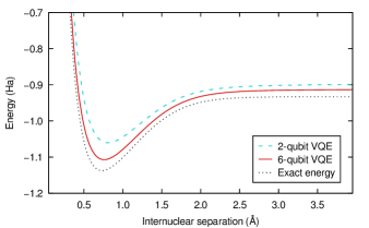
Figure 5: Energy potential curves of the $\mathrm{H}_{2}$ molecule calculated analytically using the VQE algorithm with the depolarizing noise model. The two-qubit gate error rate is $p=5\,\%$.

We analyze the effect of noise on the calculated ground-state energies using the depolarizing noise model. The noise operation for one qubit is given by [26]

$$\epsilon(\rho)=(1-p)\rho+p\frac{I}{2},$$ (6)

where $\rho$ is the density matrix and $p$ is the probabilistic error rate. The value of $p=0$ corresponds to vanishing noise and $p=1$ corresponds to full noise. We assume that the noise affects only qubits involved in a particular gate application. Separate operations are used for one-qubit gates,

$$\epsilon_{i}(\rho)=(1-p_{1})\rho+\frac{p_{1}}{4}\sum_{E_{i}\in\mathcal{P}_{i}}E_{i}^{\dagger}\rho E_{i},$$ (7)

and for two-qubit gates,

$$\epsilon_{i,j}(\rho)=(1-p_{2})\rho+\frac{p_{2}}{16}\sum_{\begin{subarray}{c}E_{i}\in\mathcal{P}_{i}\\ E_{j}\in\mathcal{P}_{j}\end{subarray}}E_{i}^{\dagger}E_{j}^{\dagger}\rho E_{i}E_{j},$$ (8)

where $\mathcal{P}_{i}=\{I_{i},X_{i},Y_{i},Z_{i}\}$ is the set of the unit matrix and the Pauli matrices acting on qubit $i$. The noise operations above are performed on the density matrix after each gate application to a respective set of qubits. We characterize the noise channel with only a single parameter $p$ and use $p_{2}=p$ and $p_{1}=p/16$ since the single-qubit gates have significantly higher fidelities in hardware. The comparison of the ground-state energy calculated with the noisy physical and encoded circuits is shown in Fig. 5. The energy error as a function of $p$ for a selected internuclear separation is shown in Fig. 6. The results show that the encoded circuit outperforms the physical circuit when the error probability of two-qubit gates is less than about $30\,\%$. This threshold is significantly higher than the error rates for two-qubit gates on the Tokyo chip which are less than $5\,\%$. Assuming that the depolarization noise model is an appropriate error model, the encoded circuit should produce a better energy estimate.

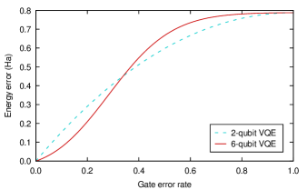
Figure 6: Energy error with the depolarizing noise model for internuclear separation $R=0.75\,\text{\AA}$. The six-qubit encoded circuit performs better for error rates up to about $30\,\%$.

Appendix C Readout error correction

Correcting measurements of discrete data for readout bias has a long history. For example, in high energy physics experiments, binned differential cross sections are corrected for detector effects in order to compare them with predictions from quantum field theory. In that context, the corrections are called unfolding (sometimes called deconvolution in other fields) and a variety of techniques have been proposed and are in active use [52, 53]. Quantum readout error correction can be represented as a binned unfolding where each bin corresponds to one of the possible $2^{n}$ configurations, where $n$ is the number of qubits.

We use an iterative Bayesian unfolding technique [54, 55, 56]. Given a response matrix

$$R_{ij}=\Pr(\text{measure}\ i\,|\,\text{truth is}\ j),$$ (9)

a measured spectrum $m_{i}=\Pr(\text{measure}\ i)$ and a prior truth spectrum $t_{i}^{0}=\Pr(\text{truth is}\ i)$, the iterative technique proceeds according to an equation

$$\begin{split}t_{i}^{l+1}&=\sum_{j}\Pr(\text{truth is}\ i\,|\,\text{measure}\ j)\times m_{j}\\ &=\sum_{j}\frac{R_{ji}t_{i}^{l}}{\sum_{k}R_{jk}t_{k}^{l}}\times m_{j},\end{split}$$ (10)

where $l$ is the iteration number. The advantage of Eq. (10) over simple matrix inversion is that the result is a probability (nonnegative and unit measure). We construct $R_{ij}$ by preparing $2^{n}$ calibration circuits where each qubit computational state is constructed with $X$ gates. The entries of $R_{ij}$ are the fraction of measurements that qubit configuration $i$ is observed in configuration $j$. We use a uniform distribution as the initial spectrum $t_{i}^{0}$. The iterative procedure described in Eq. (10) is repeated until convergence. The effect of readout error correction on potential energy curves is shown in Fig. 7. Comparison of iterative Bayesian unfolding with other available methods is discussed in Ref. [51].

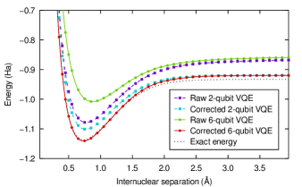
Figure 7: Comparison of potential energy curves obtained with raw measurement outcomes and with outcomes corrected for readout errors for both the two-qubit and six-qubit circuits.

Appendix D Initial state preparation

The encoded circuit uses ancilla $a_{1}$ to detect an error during the initial state preparation. Measured value zero corresponds to no error whereas one corresponds to a detected error in the state preparation. We therefore postselect only outcomes with $a_{1}$ being zero. Fig. 8 shows the effect of the postselection. About 8% of the samples were discarded due to the postselection on $a_{1}$.

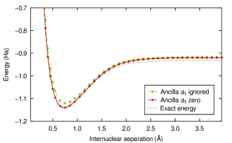
Figure 8: Comparison of potential energy curves obtained with the six-qubit circuit when ignoring the value of ancilla $a_{1}$ and when postselecting only outcomes with $a_{1}$ being zero.

Appendix E Syndrome measurement

The stabilizers of the [[4, 2, 2]] code are generated by operators $X_{1}X_{2}X_{3}X_{4}$ and $Z_{1}Z_{2}Z_{3}Z_{4}$ [30]. Code words are eigenvectors of stabilizers with $+1$ eigenvalue. A single bit-flip error in a code word transforms the code word into an eigenvector of the $Z_{1}Z_{2}Z_{3}Z_{4}$ stabilizer with $-1$ eigenvalue. A single phase-flip error transforms it into an eigenvector of the $X_{1}X_{2}X_{3}X_{4}$ stabilizer with $-1$ eigenvalue. To detect both a bit-flip and a phase-flip error, it is necessary to perform syndrome measurements in the two bases corresponding to the two stabilizer generators [27]. We do not perform these measurements in our encoded circuit. Instead, we only measure physical qubits in the computational basis. The parity of the code qubits then corresponds to the eigenvalue of one of the generators. In particular, it corresponds to $Z_{1}Z_{2}Z_{3}Z_{4}$ when $R_{t}=I$ and to $X_{1}X_{2}X_{3}X_{4}$ when $R_{t}=H$. We therefore perform only one syndrome measurement and detect only a bit-flip or a phase-flip error. A detection of both errors would require additional qubits and gates [27] or additional measurements [21]. About 11% and 16% of samples were discarded due to syndrome measurement when $R_{t}=I$ and $R_{t}=H$, respectively, for data used in the final figures. The error rate for the $\langle X_{1}X_{2}\rangle_{\theta}$ term is therefore significantly higher than for the other Hamiltonian terms.

Appendix F Qubit mappings

The availability of qubits and their connections has changed during the data collection. The final data were collected after a connection between qubits three and nine was turned off. Additionally, qubit seven was not available during experiments with the six-qubit circuit. As a result, there were only 70 and 116 possible mappings from the abstract qubits to the physical qubits for the two-qubit and the six-qubit circuits, respectively.

We found it practical to run our circuits for each of their possible mappings to find optimal mappings. However, this approach is unfeasible for larger systems. An alternative method is to estimate the total circuit fidelity from reported gate fidelities. Although we found acceptable qubit mappings using this approach, we were never able to find the best one. The action of gates is highly nontrivial and cannot be reduced to a single number. A significant error source is also cross-talk between qubits. Estimates of the total circuit fidelities therefore have only a limited reliability. Optimal qubit mapping is an area of active research [57].

References

- Reiher et al. [2017] M. Reiher, N. Wiebe, K. M. Svore, D. Wecker, and M. Troyer, Proc. Natl. Acad. Sci. U.S.A. 114, 7555 (2017).
- Preskill [2018] J. Preskill, Quantum 2, 79 (2018).
- Peruzzo et al. [2014] A. Peruzzo, J. McClean, P. Shadbolt, M.-H. Yung, X.-Q. Zhou, P. J. Love, A. Aspuru-Guzik, and J. L. O’Brien, Nat. Commun. 5, 4213 (2014).
- McClean et al. [2016] J. R. McClean, J. Romero, R. Babbush, and A. Aspuru-Guzik, New J. Phys. 18, 023023 (2016).
- O’Malley et al. [2016] P. J. J. O’Malley, R. Babbush, I. D. Kivlichan, J. Romero, J. R. McClean, R. Barends, J. Kelly, P. Roushan, A. Tranter, N. Ding, B. Campbell, Y. Chen, Z. Chen, B. Chiaro, A. Dunsworth, A. G. Fowler, E. Jeffrey, E. Lucero, A. Megrant, J. Y. Mutus, M. Neeley, C. Neill, C. Quintana, D. Sank, A. Vainsencher, J. Wenner, T. C. White, P. V. Coveney, P. J. Love, H. Neven, A. Aspuru-Guzik, and J. M. Martinis, Phys. Rev. X 6, 031007 (2016).
- Kandala et al. [2017] A. Kandala, A. Mezzacapo, K. Temme, M. Takita, M. Brink, J. M. Chow, and J. M. Gambetta, Nature 549, 242 (2017).
- Shen et al. [2017] Y. Shen, X. Zhang, S. Zhang, J.-N. Zhang, M.-H. Yung, and K. Kim, Phys. Rev. A 95, 020501 (2017).
- Colless et al. [2018] J. I. Colless, V. V. Ramasesh, D. Dahlen, M. S. Blok, M. E. Kimchi-Schwartz, J. R. McClean, J. Carter, W. A. de Jong, and I. Siddiqi, Phys. Rev. X 8, 011021 (2018).
- Dumitrescu et al. [2018] E. F. Dumitrescu, A. J. McCaskey, G. Hagen, G. R. Jansen, T. D. Morris, T. Papenbrock, R. C. Pooser, D. J. Dean, and P. Lougovski, Phys. Rev. Lett. 120, 210501 (2018).
- Hempel et al. [2018] C. Hempel, C. Maier, J. Romero, J. McClean, T. Monz, H. Shen, P. Jurcevic, B. P. Lanyon, P. Love, R. Babbush, A. Aspuru-Guzik, R. Blatt, and C. F. Roos, Phys. Rev. X 8, 031022 (2018).
- Ganzhorn et al. [2019] M. Ganzhorn, D. J. Egger, P. Barkoutsos, P. Ollitrault, G. Salis, N. Moll, M. Roth, A. Fuhrer, P. Mueller, S. Woerner, I. Tavernelli, and S. Filipp, Phys. Rev. Appl. 11, 044092 (2019).
- Kokail et al. [2019] C. Kokail, C. Maier, R. van Bijnen, T. Brydges, M. K. Joshi, P. Jurcevic, C. A. Muschik, P. Silvi, R. Blatt, C. F. Roos, and P. Zoller, Nature 569, 355 (2019).
- Li and Benjamin [2017] Y. Li and S. C. Benjamin, Phys. Rev. X 7, 021050 (2017).
- Temme et al. [2017] K. Temme, S. Bravyi, and J. M. Gambetta, Phys. Rev. Lett. 119, 180509 (2017).
- McClean et al. [2017] J. R. McClean, M. E. Kimchi-Schwartz, J. Carter, and W. A. de Jong, Phys. Rev. A 95, 042308 (2017).
- Bonet-Monroig et al. [2018] X. Bonet-Monroig, R. Sagastizabal, M. Singh, and T. E. O’Brien, Phys. Rev. A 98, 062339 (2018).
- Endo et al. [2018] S. Endo, S. C. Benjamin, and Y. Li, Phys. Rev. X 8, 031027 (2018).
- McArdle et al. [2019] S. McArdle, X. Yuan, and S. Benjamin, Phys. Rev. Lett. 122, 180501 (2019).
- Endo et al. [2019] S. Endo, Q. Zhao, Y. Li, S. Benjamin, and X. Yuan, Phys. Rev. A 99, 012334 (2019).
- Kandala et al. [2019] A. Kandala, K. Temme, A. D. Córcoles, A. Mezzacapo, J. M. Chow, and J. M. Gambetta, Nature 567, 491 (2019).
- McClean et al. [2020] J. R. McClean, Z. Jiang, N. C. Rubin, R. Babbush, and H. Neven, Nat. Commun. 11, 636 (2020).
- Otten and Gray [2019a] M. Otten and S. K. Gray, Phys. Rev. A 99, 012338 (2019a).
- Otten and Gray [2019b] M. Otten and S. K. Gray, npj Quantum Inf. 5, 11 (2019b).
- Sagastizabal et al. [2019] R. Sagastizabal, X. Bonet-Monroig, M. Singh, M. A. Rol, C. C. Bultink, X. Fu, C. H. Price, V. P. Ostroukh, N. Muthusubramanian, A. Bruno, M. Beekman, N. Haider, T. E. O’Brien, and L. DiCarlo, Phys. Rev. A 100, 010302 (2019).
- Gottesman [1997] D. E. Gottesman, Stabilizer Codes and Quantum Error Correction, Ph.D. thesis, California Institute of Technology (1997).
- Nielsen and Chuang [2010] M. A. Nielsen and I. L. Chuang, Quantum Computation and Quantum Information: 10th Anniversary Edition (Cambridge University Press, Cambridge, 2010).
- Devitt et al. [2013] S. J. Devitt, W. J. Munro, and K. Nemoto, Rep. Prog. Phys. 76, 076001 (2013).
- Terhal [2015] B. M. Terhal, Rev. Mod. Phys. 87, 307 (2015).
- Campbell et al. [2017] E. T. Campbell, B. M. Terhal, and C. Vuillot, Nature 549, 172 (2017).
- Gottesman [2016] D. Gottesman, “Quantum fault tolerance in small experiments,” arXiv (2016), arXiv:1610.03507 [quant-ph] .
- Chao and Reichardt [2018a] R. Chao and B. W. Reichardt, Phys. Rev. Lett. 121, 050502 (2018a).
- Chao and Reichardt [2018b] R. Chao and B. W. Reichardt, npj Quantum Inf. 4, 42 (2018b).
- Reed et al. [2012] M. D. Reed, L. DiCarlo, S. E. Nigg, L. Sun, L. Frunzio, S. M. Girvin, and R. J. Schoelkopf, Nature 482, 382 (2012).
- Nigg et al. [2014] D. Nigg, M. Müller, E. A. Martinez, P. Schindler, M. Hennrich, T. Monz, M. A. Martin-Delgado, and R. Blatt, Science 345, 302 (2014).
- Barends et al. [2014] R. Barends, J. Kelly, A. Megrant, A. Veitia, D. Sank, E. Jeffrey, T. C. White, J. Mutus, A. G. Fowler, B. Campbell, Y. Chen, Z. Chen, B. Chiaro, A. Dunsworth, C. Neill, P. O’Malley, P. Roushan, A. Vainsencher, J. Wenner, A. N. Korotkov, A. N. Cleland, and J. M. Martinis, Nature 508, 500 (2014).
- Kelly et al. [2015] J. Kelly, R. Barends, A. G. Fowler, A. Megrant, E. Jeffrey, T. C. White, D. Sank, J. Y. Mutus, B. Campbell, Y. Chen, Z. Chen, B. Chiaro, A. Dunsworth, I.-C. Hoi, C. Neill, P. J. J. O’Malley, C. Quintana, P. Roushan, A. Vainsencher, J. Wenner, A. N. Cleland, and J. M. Martinis, Nature 519, 66 (2015).
- Wootton and Loss [2018] J. R. Wootton and D. Loss, Phys. Rev. A 97, 052313 (2018).
- Linke et al. [2017] N. M. Linke, M. Gutierrez, K. A. Landsman, C. Figgatt, S. Debnath, K. R. Brown, and C. Monroe, Sci. Adv. 3, e1701074 (2017).
- Takita et al. [2017] M. Takita, A. W. Cross, A. D. Córcoles, J. M. Chow, and J. M. Gambetta, Phys. Rev. Lett. 119, 180501 (2017).
- Roffe et al. [2018] J. Roffe, D. Headley, N. Chancellor, D. Horsman, and V. Kendon, Quantum Sci. Technol. 3, 035010 (2018).
- Vuillot [2018] C. Vuillot, Quantum Inf. Comput. 18, 0949 (2018).
- Willsch et al. [2018] D. Willsch, M. Willsch, F. Jin, H. De Raedt, and K. Michielsen, Phys. Rev. A 98, 052348 (2018).
- Harper and Flammia [2019] R. Harper and S. T. Flammia, Phys. Rev. Lett. 122, 080504 (2019).
- Vaidman et al. [1996] L. Vaidman, L. Goldenberg, and S. Wiesner, Phys. Rev. A 54, R1745 (1996).
- Grassl et al. [1997] M. Grassl, T. Beth, and T. Pellizzari, Phys. Rev. A 56, 33 (1997).
- Jordan and Wigner [1928] P. Jordan and E. Wigner, Z. Phys. 47, 631 (1928).
- Bravyi and Kitaev [2002] S. B. Bravyi and A. Y. Kitaev, Ann. Phys. (N. Y.) 298, 210 (2002).
- Bartlett et al. [1989] R. J. Bartlett, S. A. Kucharski, and J. Noga, Chem. Phys. Lett. 155, 133 (1989).
- Taube and Bartlett [2006] A. G. Taube and R. J. Bartlett, Int. J. Quantum Chem. 106, 3393 (2006).
- Yeter-Aydeniz et al. [2019] K. Yeter-Aydeniz, E. F. Dumitrescu, A. J. McCaskey, R. S. Bennink, R. C. Pooser, and G. Siopsis, Phys. Rev. A 99, 032306 (2019).
- Nachman et al. [2019] B. Nachman, M. Urbanek, W. A. de Jong, and C. W. Bauer, “Unfolding quantum computer readout noise,” arXiv (2019), arXiv:1910.01969 [quant-ph] .
- Cowan [2002] G. Cowan, Advanced Statistical Techniques in Particle Physics, Durham, UK, March 18–22, 2002, Conf. Proc. C0203181, 248 (2002).
- Blobel [2013] V. Blobel, in Data Analysis in High Energy Physics (John Wiley & Sons, 2013) pp. 187–225.
- Lucy [1974] L. B. Lucy, Astron. J. 79, 745 (1974).
- Richardson [1972] W. H. Richardson, J. Opt. Soc. Am. 62, 55 (1972).
- D’Agostini [1995] G. D’Agostini, Nucl. Instrum. Methods Phys. Res. A 362, 487 (1995).
- Murali et al. [2019] P. Murali, J. M. Baker, A. Javadi-Abhari, F. T. Chong, and M. Martonosi, in Proceedings of the Twenty-Fourth International Conference on Architectural Support for Programming Languages and Operating Systems, ASPLOS ’19 (Association for Computing Machinery, 2019) pp. 1015–1029.