Accuracy Prevents Robustness in Perception-based Control

Abstract

In this paper we prove the existence of a fundamental trade-off between accuracy and robustness in perception-based control, where control decisions rely solely on data-driven, and often incompletely trained, perception maps. In particular, we consider a control problem where the state of the system is estimated from measurements extracted from a high-dimensional sensor, such as a camera. We assume that a map between the camera’s readings and the state of the system has been learned from a set of training data of finite size, from which the noise statistics are also estimated. We show that algorithms that maximize the estimation accuracy (as measured by the mean squared error) using the learned perception map tend to perform poorly in practice, where the sensor’s statistics often differ from the learned ones. Conversely, increasing the variability and size of the training data leads to robust performance, however limiting the estimation accuracy, and thus the control performance, in nominal conditions. Ultimately, our work proves the existence and the implications of a fundamental trade-off between accuracy and robustness in perception-based control, which, more generally, affects a large class of machine learning and data-driven algorithms [1, 2, 3, 4].

I Introduction

Machine learning methods are rapidly being deployed for a broad class of applications, ranging from speech recognition and malware detection, to control design and dynamic decision making. These data-driven algorithms often outperform classical methods and require, typically, substantially less knowledge about the specifics of the problem. For control applications, in particular, data-driven algorithms promise to overcome the limitations of traditional model-based approaches, and to provide solutions to complex control problems where a detailed model of the plant and its operating environment is either too complex to be useful, or too difficult to estimate or derive from first principles [5, 6, 7]. Yet, the lack of strong guarantees for the safety and robustness of data-driven algorithms questions their deployment, especially in applications such as autonomous driving and exploration.

In this paper, we characterize a fundamental trade-off between accuracy and robustness in a data-driven control problem. We consider a perception-based control scenario, Fig. 1, where a camera is used to partially measure the state of a dynamical system and construct an estimator of the full state. We assume that the output map between the high-dimensional camera stream and the system state has been learned accurately [8], although the estimated statistics of the measurement noise are inaccurate. Such inaccuracies, which can arise from limited training data, sudden changes in environmental conditions, and adversarial manipulation, are unknown to the estimator and induce incorrect confidence bounds on the estimated state variables. In turn, inaccurate confidence bounds can lead to harmful control decisions [9]. Further, we show that, because of the incorrect noise statistics, accuracy of the estimation algorithm can be improved only at the expenses of its robustness. Thus, estimation algorithms that are optimal in the nominal training phase may underperform in practice compared to suboptimal algorithms. Our analytical results provide an explanation as to why nominally suboptimal data-driven algorithms can exhibit better generalization and robust properties in practice [10].

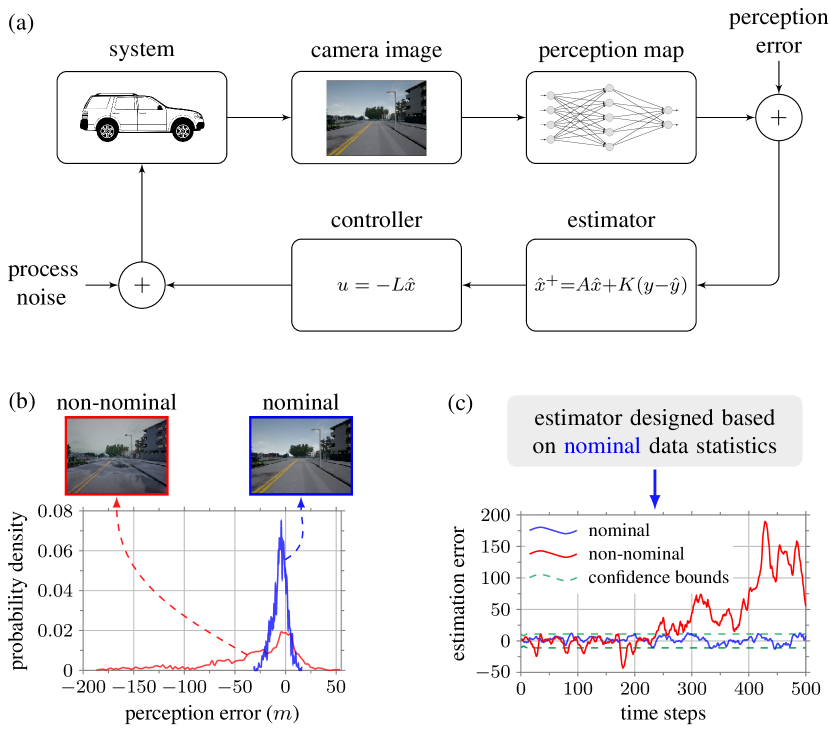
Figure 1: Panel (a) shows a perception-based control scenario, where the partial state of a dynamical system (vehicle) is extracted from the measurements of a high-dimensional sensor (camera) and used to implement a feedback control algorithm. A perception map is learned from a set of training data of finite size, which relates the sensor’s readings to the system’s state. Panel (b) shows the probability density functions of the perception error when operating in nominal (clear weather, as represented by the training data) and non-nominal (rainy weather, as it may occur in practice) conditions (error statistics are computed numerically using the simulator CARLA [11]). Due to inaccuracies and uncertainties in the sensed data, the error statistics of the perception map differ from the statistics learned during the training phase. As shown in panel (c), discrepancies in the error statistics lead to poor estimation performance in practical conditions. As we prove in this paper, a fundamental trade-off exists between accuracy and robustness of a linear estimator (consequently, in the considered perception-based control setting), so that estimators that perform well on the training data may exhibit poor performance with non-nominal conditions, while robust estimators may exhibit mediocre yet robust performance in a broad set of conditions.

Related work. Machine learning and, more generally, data-driven algorithms have shown remarkable performance under nominal and well-modeled conditions in a variety of applications. Yet, the same algorithms have proven extremely fragile when subject to small, yet targeted, perturbations of the data [12, 13]. A detailed understanding of this unreliable behavior is still lacking, with recent theoretical results proving robustness and generalization guarantees for learning algorithms subject to adversarial disturbances, e.g., see [14, 15, 16], and showing that, in certain contexts, robustness to perturbations and performance under nominal conditions are inversely related [1, 2, 3, 4]. Compared to these works, we prove that a fundamental trade-off between accuracy and robustness also arises in linear estimation algorithms, which may lead to a critical degradation of the closed loop performance [9].

Related to this work is the literature on robust control and estimation [17, 18]. However, the primary focus of this paper is not on designing a robust estimator or controller, but rather on proving the existence of a fundamental trade-off between accuracy and robustness, which plays a critical role in the deployment of learning and data-driven methods in control applications, including perception-based control.

Finally, the literature on perception-based control is also very rich, with results ranging from integrating camera measurements with inertial odometry [19], to control of unmanned aerial vehicles [20] and vision-based planning [21], to name a few. To the best of our knowledge, the trade-off between accuracy and robustness that we highlight here was not discussed in any of the above research streams.

Paper contributions. This paper features two main contributions. First, we study a perception-based control problem, where the state of a dynamical system is reconstructed using a high-dimensional sensor. We prove the existence of a fundamental trade-off between the accuracy of the estimation algorithm, as measured by its minimum mean squared error, and its robustness to variations and inaccuracies of the data statistics. Thus, (i) estimation algorithms that are optimal for the nominal data tend to perform poorly in practice, where the operating conditions may differ from the nominal data, and, conversely, (ii) estimation algorithms that are robust to data variations exhibit suboptimal performance in nominal conditions. Second, we characterize estimators that lie on the Pareto frontier between accuracy and robustness, that is, estimators that are maximally robust for a desired performance level, and estimators that are maximally accurate for a given bound on the data variations and inaccuracies. We also show, numerically, that the trade-off for estimation algorithms also affects the performance of the closed-loop system, and even when the measurement error is not normally distributed, as we assume for the derivation of our analytical results.

In a broader context, the results of this paper further characterize a fundamental limitation of machine learning and data-driven algorithms, as described for different settings in [1, 2, 3, 4], and clarify its implications for control applications.

Paper’s organization. The rest of the paper is organized as follows. Section II contains our mathematical setup. Section III contains the trade-off between accuracy and robustness, and the design of optimal estimators. Section IV contains our numerical example, and Section V concludes the paper.

Notation. A Gaussian random variable $x$ with mean $\mu$ and covariance $\Sigma$ is denoted as $x\sim\mathcal{N}(\mu,\Sigma)$. The $n\times n$ identity matrix is denoted by $I_{n}$. The expectation operator is denoted by $\mathbb{E}[\cdot]$. The spectral radius and the trace of a square matrix $A$ are denoted by $\rho(A)$ and $\mathsf{Tr}(A)$, respectively. A positive definite (semidefinite) matrix $A$ is denoted as $A>0$ ($A\geq 0$). The Kronecker product is denoted by $\otimes$, and vectorization operator is denoted by vec($\cdot$).

II Problem setup and preliminary notions

Consider the discrete-time, linear, time-invariant system

$$x(t+1) =Ax(t)+w(t),$$ (1)

$$y(t) =Cx(t)+v(t),\qquad t\geq 0,$$ (2)

where $x(t)\in\mathbb{R}^{n}$ denotes the state, $y(t)\in\mathbb{R}^{m}$ the output, $w(t)$ the process noise, and $v(t)$ the measurement noise. We assume that $w(t)\sim\mathcal{N}(0,Q)$, with $Q\geq 0$, $v(t)\sim\mathcal{N}(0,R)$, with $R>0$, and $x(0)\sim\mathcal{N}(0,\Sigma_{0})$, with $\Sigma_{0}\geq 0$, are independent of each other at all times $t\geq 0$. Finally, we assume that $A$ is stable, that is, $\rho(A)<1$. Note that this implies that $(A,C)$ is detectable and $(A,Q^{\frac{1}{2}})$ is stabilizable.

We use a linear filter with constant gain $K\in\mathbb{R}^{n\times m}$ to estimate the state of the system (1) from the measurements (2):

$$\hat{x}(t+1)=A\hat{x}(t)+K[y(t+1)-CA\hat{x}(t)]\quad t\geq 0,$$ (3)

where $\hat{x}(t)$ denotes the state estimate at time $t$. Let $e(t)=x(t)-\hat{x}(t)$ and $P(t)=\mathbb{E}[e(t)e(t)^{\mathsf{T}}]$ denote the estimation error and its covariance, respectively. For $t\geq 0$, we have

$$e(t+1) =A_{K}e(t)+B_{K}w(t)-Kv(t+1),$$ (4)

$$P(t+1) =A_{K}P(t)A_{K}^{\mathsf{T}}+B_{K}QB_{K}^{\mathsf{T}}+KRK^{\mathsf{T}},$$ (5)

where $A_{K}\triangleq A-KCA$ and $B_{K}\triangleq I_{n}-KC$. We assume that the gain $K$ is chosen such that $A_{K}$ is stable, that is, $\rho(A_{K})<1$. Under this assumption, $\underset{t\rightarrow\infty}{\lim}P(t)\triangleq P(K)\geq 0$ exists, and satisfies the Lyapunov equation

$$P(K)=A_{K}P(K)A_{K}^{\mathsf{T}}+B_{K}QB_{K}^{\mathsf{T}}+KRK^{\mathsf{T}}.$$ (6)

The performance of the filter is quantified by $\mathcal{P}(K)\triangleq\mathsf{Tr}(P(K))$, where a lower value of $\mathcal{P}(K)$ is desirable. Note that the steady-state gain ${K}_{\textup{kf}}$ of the Kalman filter [22] minimizes $\mathcal{P}(K)$ and depends on the matrices $A$, $C$, $Q$, $R$.

We allow for perturbations to the covariance matrix $R$, which may result from (i) modeling and estimation errors, as in the case of perception-based control, or (ii) accidental or adversarial tampering of the sensor, as in the case of false data injection attacks [23]. To quantify the effect of such perturbations to the covariance matrix $R$ on the performance of the estimator, we define the following sensitivity metric:

$$\mathcal{S}(K)\triangleq\mathsf{Tr}\left[\frac{d}{dR}\mathcal{P}(K)\right].$$ (7)

Intuitively, if $\mathcal{S}(K)$ is large, then a small change in $R$ can result in a large change (possibly, large increment) in $\mathcal{P}(K)$.

Remark 1

(Comparison with adversarial robustness) In adversarial settings, the adversary designs a small deterministic perturbation added to a given observation (e.g., pixels of an image) to deteriorate the performance of a machine learning algorithm. This perturbed observation can be viewed as a realization of a multi-dimensional distribution. Instead, in this work we consider perturbations to the sensor’s noise covariance, which accounts for all possible realizations. Thus, our sensitivity metric captures the average performance change over all possible perturbations, rather than the degradation caused by a single worst-case perturbation.  $\square$

Lower values of sensitivity $\mathcal{S}(K)$ are desirable, and indicate that the filter (3) is more robust to perturbations. This motivates the following optimization problem:

$$\mathcal{S}^{*}(\delta)= \;\underset{K}{\min}\quad\mathcal{S}(K)$$ (8)

$$\;\text{s.t.}\quad\mathcal{P}(K)\leq\delta,$$

where $\delta\geq\mathcal{P}({K}_{\textup{kf}})$ for feasibility. In what follows, we characterize the solution $K^{*}$ to (8), and the relations between the sensitivity $\mathcal{S}(K^{*})$ and the error $\mathcal{P}(K^{*})$ as $\delta$ varies. To facilitate the discussion, in the remainder of the paper we use accuracy to refer to any decreasing function of the error $\mathcal{P}(K)$ obtained by the gain $K$, and robustness to denote any decreasing function of the sensitivity $\mathcal{S}(K)$ of the gain $K$.

III Accuracy vs robustness trade-off in
linear estimation algorithms

We begin by characterizing the sensitivity $\mathcal{S}(K)$.

Lemma III.1

(Characterization of sensitivity) Let the sensitivity $\mathcal{S}(K)$ be as in (7). Then, $\mathcal{S}(K)=\mathsf{Tr}(S(K))$, where $S(K)\geq 0$ satisfies the following Lyapunov equation:

$$S(K)=A_{K}S(K)A_{K}^{\mathsf{T}}+KK^{\mathsf{T}}.$$ (9)

Lemma III.1 allows us to compute the sensitivity of the linear estimator (3) as a function of its gain. Before proving Lemma III.1, we present the following technical result.

Lemma III.2

(Property of the solution to Lyapunov equation) Let $A$, $B$, $Q$ be matrices of appropriate dimension with $\rho(A)<1$. Let $Y$ satisfy $Y=AYA^{\mathsf{T}}+Q$. Then, $\mathsf{Tr}(BY)=\mathsf{Tr}(Q^{\mathsf{T}}M)$, where $M$ satisfies $M=A^{\mathsf{T}}MA+B^{\mathsf{T}}$.

Proof:

Since $\rho(A)<1$, $Y$ and $M$ can be written as

$$Y=\sum_{i=0}^{\infty}A^{i}Q(A^{\mathsf{T}})^{i}\text{ and }M=\sum_{i=0}^{\infty}A^{i}B(A^{\mathsf{T}})^{i}.$$ (10)

The result follows by pre-multiplying $Y$ and $M$ by $B$ and $Q^{\mathsf{T}}$ respectively, and using the cyclic property of trace. ∎

Proof of Lemma III.1:   Taking the differential of $\eqref{eq: lyapunov equation error covariance}$ with respect to the variable $R$, we get

$$dP(K) =A_{K}dP(K)A_{K}^{\mathsf{T}}+KdRK^{\mathsf{T}}$$

$$\Rightarrow d\mathsf{Tr}(P(K)) =\mathsf{Tr}(dP(K))\overset{(a)}{=}\mathsf{Tr}(KdRK^{\mathsf{T}}M),$$ (11)

where $M>0$ satisfies: $M=A_{K}^{\mathsf{T}}MA_{K}+I_{n}$, and $(a)$ follows from Lemma III.2. From (11), we get

$$d\mathcal{P}(K)=\mathsf{Tr}(K^{\mathsf{T}}MKdR)\Rightarrow\frac{d}{dR}\mathcal{P}(K)=K^{\mathsf{T}}MK.$$ (12)

Using (12) and (7), we have that $\mathcal{S}(K)=\mathsf{Tr}(K^{\mathsf{T}}MK)=\mathsf{Tr}(KK^{\mathsf{T}}M)=\mathsf{Tr}(S(K))$, where $S(K)$ is defined in (9) and the last equality follows from Lemma III.2. To conclude, the property $S(K)\geq 0$ follows by inspection from (9). $\blacksquare$

Notice that, since $S(K)\geq 0$, $\mathcal{S}(K)=\mathsf{Tr}(S(K))$ is a valid norm of $S(K)$ and captures the size of $S(K)$. Further, $S(K)=0$ for $K=0$, that is, $K=0$ achieves the lowest possible value of sensitivity. This implies that $\delta$ in the optimization problem (8) can be restricted to $[\mathcal{P}(K_{\text{kf}}),\mathcal{P}(0)]$ to characterize the accuracy-robustness trade-off.

Next, we characterize the optimal solution to (8). We will show that, despite not being convex, the minimization problem (8) exhibits a unique local minimum. This implies that the local minimum is also the global minimum.

Theorem III.3

(Solution to the minimization problem (8)) Let $\delta\in[\mathcal{P}(K_{\text{kf}}),\mathcal{P}(0)]$ and $\lambda\geq 0$. Let $X\geq 0$ be the unique solution to the following Riccati equation:

$$X=AXA^{\mathsf{T}}\!-\!AXC^{\mathsf{T}}(CXC^{\mathsf{T}}\!+\!I_{m}\!+\!\lambda R)^{-1}CXA^{\mathsf{T}}\!+\!\lambda Q.$$ (13)

Then, the global minimum of problem (8) is given by

$$K^{*}(\lambda)=XC^{\mathsf{T}}\Big{(}CXC^{\mathsf{T}}+I_{m}+\lambda R\Big{)}^{-1},$$ (14)

where $\lambda$ is selected such that $\mathcal{P}(K^{*}(\lambda))\triangleq\mathcal{P}^{*}(\lambda)=\delta$.

Proof:

First-order necessary conditions: We begin by computing the derivatives of $\mathcal{P}(K)$ and $\mathcal{S}(K)$ with respect to the variable $K$. For notational convenience, we denote $A_{K},B_{K},P(K)$ and $S(K)$ by $\bar{A},B,P$ and $S$, respectively. Taking the differential of (9), we get

$$dS =\bar{A}dS\bar{A}^{\mathsf{T}}-dKCAS\bar{A}^{\mathsf{T}}-\bar{A}S(dKCA)^{\mathsf{T}}+dKK^{\mathsf{T}}$$

$$+KdK^{\mathsf{T}}\triangleq\bar{A}dS\bar{A}^{\mathsf{T}}+Z$$ (15)

$$\Rightarrow d\mathcal{S}(K)\overset{(a)}{=}\mathsf{Tr}(dS)\overset{(b)}{=}\mathsf{Tr}(Z^{\mathsf{T}}M)$$

$$=2\mathsf{Tr}[(-CAS\bar{A}^{\mathsf{T}}+K^{\mathsf{T}})MdK]$$

$$\Rightarrow\frac{d}{dK}\mathcal{S}(K)=2M(K-\bar{A}SA^{\mathsf{T}}C^{\mathsf{T}}),$$ (16)

where $M>0$ satisfies $M=A_{K}^{\mathsf{T}}MA_{K}+I_{n}$, and $(a)$ and $(b)$ follow from Lemmas III.1 and III.2, respectively. A similar analysis of (6) yields

$$\frac{d}{dK}\mathcal{P}(K)=2M(KR-\bar{A}PA^{\mathsf{T}}C^{\mathsf{T}}-BQC^{\mathsf{T}}).$$ (17)

Define the Lagrange function of problem (8) as

$$\mathcal{L}(K,\lambda)=\mathcal{S}(K)+\lambda\Big{(}\mathcal{P}(K)-\delta\Big{)},$$ (18)

where $\lambda$ is the Karush-Kuhn-Tucker (KKT) multiplier. The stationary KKT condition implies $\frac{d}{dK}\mathcal{L}(K,\lambda)=0$, which using (16) and (17) becomes

$$2M[K-\bar{A}SA^{\mathsf{T}}C^{\mathsf{T}}+\lambda(KR-\bar{A}PA^{\mathsf{T}}C^{\mathsf{T}}-BQC^{\mathsf{T}})]=0.$$ (19)

Substituting $\bar{A}=A-KCA$ in the above equation, defining $X\triangleq A(S+\lambda P)A^{\mathsf{T}}+\lambda Q$, and using $M>0$, we obtain (14). Next, we show that $X$ satisfies (13). From (6) and (9):

$$S+\lambda P=\bar{A}(S+\lambda P)\bar{A}^{\mathsf{T}}+\lambda BQB^{\mathsf{T}}+K(I_{m}+\lambda R)K^{\mathsf{T}}$$

$$\Rightarrow X=A(S+\lambda P)A^{\mathsf{T}}+\lambda Q$$

$$=A\left[\bar{A}(S+\lambda P)\bar{A}^{\mathsf{T}}+\lambda BQB^{\mathsf{T}}+K(I_{m}+\lambda R)K^{\mathsf{T}}\right]A^{\mathsf{T}}$$

$$\;\;\;\;+\lambda Q.$$

Using $\bar{A}=A-KCA$ and substituting the gain $K$ in (14) in the above equation, we obtain the Riccati equation (13).

The KKT condition for dual feasibility implies that $\lambda\geq 0$, so (13) has a unique stabilizing solution. Further, the KKT condition for complementary slackness implies $\lambda[\mathcal{P}(K^{*}(\lambda))-\delta]=0$. Thus, if $\lambda>0$, then $\mathcal{P}(K^{*}(\lambda))=\delta$. If $\lambda=0$, then the solution to (13) is $X=0$. This implies that $K^{*}(0)=0$, which is feasible only if $\delta=\mathcal{P}(0)$. Thus, for any $\delta\in[\mathcal{P}(K_{\text{kf}}),\mathcal{P}(0)]$, it holds $\mathcal{P}(K^{*}(\lambda))=\delta$.

Second-order sufficient conditions: We show that the stationary point (14) corresponds to a local minimum. We begin by computing the second-order differential of $\mathcal{S}(K)$. Taking the differential of (III) and noting that $d^{2}K=0$, we get

$$d^{2}S =\bar{A}d^{2}S\bar{A}^{\mathsf{T}}-2dKCAdS\bar{A}^{\mathsf{T}}-2\bar{A}dS(dKCA)^{\mathsf{T}}$$

$$+2dK(I_{p}+CASA^{\mathsf{T}}C^{\mathsf{T}})dK^{\mathsf{T}}\triangleq\bar{A}d^{2}S\bar{A}^{\mathsf{T}}+Y$$

$$\Rightarrow d^{2}\mathcal{S}(K) =\mathsf{Tr}(d^{2}S)=\mathsf{Tr}(YM)=-4\mathsf{Tr}(dKCAdS\bar{A}^{\mathsf{T}}M)$$

$$+2\mathsf{Tr}(dK(I_{p}+CASA^{\mathsf{T}}C^{\mathsf{T}})dK^{\mathsf{T}}M).$$ (20)

Similar analysis of (6) yields

$$d^{2}\mathcal{P}(K) =-4\mathsf{Tr}(dKCAdP\bar{A}^{\mathsf{T}}M)$$ (21)

$$+2\mathsf{Tr}[dK(R+CAPA^{\mathsf{T}}C^{\mathsf{T}}+CQC^{\mathsf{T}})dK^{\mathsf{T}}M].$$

Adding (20) and (21), we get

$$d^{2}{\mathcal{L}}=-4\mathsf{Tr}(dKCA\underbrace{(dS+\lambda dP)}_{\overset{(a)}{=}0.}\bar{A}^{\mathsf{T}}M)$$

$$+2\mathsf{Tr}[dKWdK^{\mathsf{T}}M]=\text{vec}^{\mathsf{T}}(dK)(2W\otimes M)\text{vec}(dK),$$

where $W\triangleq I_{p}+\lambda R+CA(S+\lambda P)A^{\mathsf{T}}C^{\mathsf{T}}+\lambda CQC^{\mathsf{T}}$, and where $(a)$ holds because $d\mathcal{L}(K,\lambda)=0$ at the stationary point. The above expression implies that the Hessian of the Lagrangian is given by $H=2W\otimes M$, which is positive-definite because $W>0$ and $M>0$. Thus, the considered stationary point corresponds to a local minimum.

Uniqueness of $\lambda$: Next, we show that for a given $\delta$, the equation $\mathcal{P}(K^{*}(\lambda))=\delta$ has a unique solution. Note that for a given $\lambda>0$, the optimal gain $K^{*}(\lambda)$ in (14) is the unique minimizer of the cost $\mathcal{C}(K)=\mathcal{S}(K)+\lambda\mathcal{P}(K)$. Let $\lambda_{2}>\lambda_{1}>0$. Then, we have

$$\mathcal{S}(K^{*}(\lambda_{1}))+\lambda_{1}\mathcal{P}(K^{*}(\lambda_{1}))<\mathcal{S}(K^{*}(\lambda_{2}))+\lambda_{1}\mathcal{P}(K^{*}(\lambda_{2})),$$

$$\mathcal{S}(K^{*}(\lambda_{2}))+\lambda_{2}\mathcal{P}(K^{*}(\lambda_{2}))<\mathcal{S}(K^{*}(\lambda_{1}))+\lambda_{2}\mathcal{P}(K^{*}(\lambda_{1})).$$

Adding the above two equations, we get $\mathcal{P}(K^{*}(\lambda_{2}))<\mathcal{P}(K^{*}(\lambda_{1}))$. Thus, $\mathcal{P}(K^{*}(\lambda))$ is a strictly decreasing function of $\lambda$, and therefore, it is one-to-one.

To conclude the proof, since the necessary and sufficient conditions for a local minimum are satisfied by a unique gain, the local minimum is also the global minimum. ∎

Corollary III.4

(Properties of $\mathcal{P}^{*}(\lambda)$) The error $\mathcal{P}^{*}(\lambda)$ defined in Theorem III.3 is a strictly decreasing function of $\lambda$.

Theorem III.3 shows that the optimal gain can be characterized in terms of a scalar parameter $\lambda$, which depends on the performance level $\delta$ according to the relation $\mathcal{P}^{*}(\lambda)=\delta$. Notice that $\lambda=0$ if $\delta=\mathcal{P}(0)$, and $\lambda$ approaches infinity as $\delta$ approaches $\mathcal{P}({K}_{\textup{\text{kf}}})$. In other words, $\underset{\lambda\rightarrow\infty}{\lim}K^{*}(\lambda)={K}_{\textup{kf}}$. Further, Corollary III.4 implies that for a given $\delta$, the solution of $\mathcal{P}^{*}(\lambda)=\delta$ can be found efficiently. For instance, one can use the bisection algorithm on the interval $[0,{\lambda}_{\textup{max}}]$, where $\mathcal{P}^{*}({\lambda}_{\textup{max}})>\delta$. These results also imply a fundamental trade-off between performance and robustness of the estimator.

Theorem III.5

(Accuracy vs robustness trade-off) Let $\mathcal{S}^{*}(\delta)$ denote the solution of (8). Then, $\mathcal{S}^{*}(\delta)$ is a strictly decreasing function of $\delta$ in the interval $\delta\in[\mathcal{P}({K}_{\textup{kf}}),\mathcal{P}(0)]$.

Proof:

From the proof of Theorem III.3, we have

$$\frac{\partial\mathcal{S}(K)}{\partial K}\Bigg{|}_{K^{*}(\lambda)}=-\lambda\frac{\partial\mathcal{P}(K)}{\partial K}\Bigg{|}_{K^{*}(\lambda)}.$$ (22)

Since $\lambda>0$ for $\delta\in[\mathcal{P}(K_{\text{kf}}),\mathcal{P}(0)]$ and $\mathcal{P}^{*}(\lambda)=\delta$, (22) implies that the sensitivity decreases when the error increases, and vice versa, so that a strict trade-off exists. ∎

Theorem III.5 implies that there exists a fundamental trade-off between the accuracy and robustness of a linear filter against perturbations to measurement noise covariance matrix. Therefore, the robustness of the linear filter in (3) in uncertain or adversarial environments can be improved only at the expenses of its accuracy in nominal conditions. Conversely, improving the robustness of the filter leads to a lower accuracy in nominal conditions.

Remark 2

(Design of optimally robust filters) Let $\Delta R\geq 0$ denote a sufficiently small perturbation to $R$ such that the approximation $\Delta\mathcal{P}(K)\approx\mathsf{Tr}(K^{\mathsf{T}}MK\Delta R)$ holds (see (12)). Further, let $\Delta R$ be bounded as $\mathsf{Tr}(\Delta R)\leq\gamma$. Then, we have

$$\Delta\mathcal{P}(K) =\mathsf{Tr}(K^{\mathsf{T}}MK\Delta R)\leq\mathsf{Tr}(K^{\mathsf{T}}MK)\rho(\Delta R)$$

$$=\mathsf{Tr}(S(K))\rho(\Delta R)\leq\gamma\mathcal{S}(K).$$

Thus, given a gain $K$, the worst case performance degradation due to a bounded perturbation to $R$ is given by ${\mathcal{P}}_{\textup{worst}}(K)=\mathcal{P}(K)+\gamma\mathcal{S}(K)$. Therefore, a filter that is optimally robust (that is, it exhibits optimal worst-case performance in the presence of norm-bounded perturbations of the noise statistics) can be obtained by minimizing ${\mathcal{P}}_{\textup{worst}}(K)$. Note that this minimization problem is akin to the problem (8), and that its solution is given by (14) with $\lambda=\gamma^{-1}$. $\square$

Remark 3

(Analysis when the system matrix $A$ is unstable) The accuracy-robustness trade-off shown above also holds when $A$ is unstable and $(A,C)$ is detectable. The analysis for this case follows the same reasoning as above, except that the range of interest for the error becomes $\delta\in[\mathcal{P}({K}_{\textup{kf}}),\mathcal{P}(K^{*}_{\mathcal{S}})]$, with $K^{*}_{\mathcal{S}}=\arg\underset{K}{\min}\>\mathcal{S}(K).$ If $A$ does not have eigenvalues on the unit circle, then the Riccati equation (13) has a unique solution for $\lambda=0$ [24] (Theorem 12.6.2), and $K^{*}_{\mathcal{S}}=K^{*}(0)$ (c.f. (14)). In this case, $\mathcal{P}(K^{*}_{\mathcal{S}})$ is finite. The case when $A$ has eigenvalues on the unit circle is more involved, finding $K^{*}_{\mathcal{S}}$ is not trivial, and $\mathcal{P}(K^{*}_{\mathcal{S}})$ may become arbitrarily large. This aspect is left for future research (see Section IV for an example with unit eigenvalues). $\square$

We conclude this section with an illustrative example.

Example 1

(Robustness versus performance trade-off) Consider the system in (1) and (2) with matrices

$$A =\begin{bmatrix}0.9&0\\ 0.02&0.8\end{bmatrix},\qquad C=\begin{bmatrix}0.5&-0.8\\ 0&0.7\end{bmatrix},$$ (23)

$$Q =\begin{bmatrix}0.5&0\\ 0&0.7\end{bmatrix},\hskip 25.6073ptR=\begin{bmatrix}0.5&0.1\\ 0.1&0.8\end{bmatrix}.$$

Fig. 2(a) shows the values $\mathcal{S}^{*}(\delta)$ obtained from (8) over the range $\delta\in[\mathcal{P}(K_{\text{kf}}),\mathcal{P}(0)]$. Several comments are in order. First, as predicted by Theorem III.5, the plot shows a trade-off between accuracy and robustness. Second, in accordance with Theorem III.3, the solution to the minimization problem (8) implies that the equality constraint in (8) is active. Third, when $\delta=\mathcal{P}({K}_{\textup{\text{kf}}})$, the minimization problem (8) returns the Kalman gain. Fourth, although the Kalman filter (depicted by the red dot) achieves the highest accuracy, it features the highest sensitivity (thus, lowest robustness) among the solutions of (8) over the range $\delta\in[\mathcal{P}({K}_{\textup{\text{kf}}}),\mathcal{P}(0)]$. Thus, the estimator that is most accurate on the nominal data, is also the most sensitive to perturbations. Fifth, the linear filter obtained when $\delta=\mathcal{P}(0)$ exhibits the worst nominal performance, but is the most robust to changes in the noise statistics. Fig. 2(b) shows the values of $\mathcal{P}^{*}(\lambda)$ as a function of $\lambda$. We observe that $\mathcal{P}^{*}(\lambda)$ is a strictly decreasing function in $\lambda$ in accordance with Corollary III.4. We also observe that the linear filter obtained when $\delta=\mathcal{P}(0)$, depicted by the green dot, has $\lambda=0$. Finally, the value $\mathcal{P}^{*}(\lambda)$ obtained when $\delta=\mathcal{P}(K_{\text{kf}})$ cannot be shown since it requires $\lambda=\infty$.  $\square$

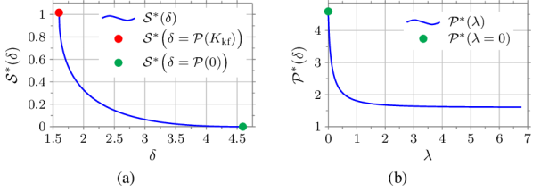
Figure 2: Panel (a) shows the accuracy versus robustness trade-off for the linear estimator (3) and the system described in Example 1. The red dot denotes the Kalman filter, and the green dot denotes the linear filter with zero gain. The Kalman filter achieves optimal performance with the nominal data, yet it is the most sensitive to changes of the noise statistics. The opposite trade-off holds for the filter with zero gain. Panel (b) shows the estimation error as a function of $\lambda$ for the system described in Example 1. The green dot denotes the filter with zero gain. The performance of the Kalman filter does not appear in the plot since it requires $\lambda=\infty$.

IV Accuracy versus robustness trade-off in perception-based control

In this section we illustrate the implication of our theoretical results to the perception-based control setting shown in Fig. 1. We consider a vehicle obeying the dynamics [8]

$$x(t+1)\!=\!\underbrace{\begin{bmatrix}1&T_{s}&0&0\\ 0&1&0&0\\ 0&0&1&T_{s}\\ 0&0&0&1\end{bmatrix}}_{A}x(t)\!+\!\underbrace{\begin{bmatrix}0&0\\ T_{s}&0\\ 0&0\\ 0&T_{s}\end{bmatrix}}_{B}u(t)\!+\!w(t),$$ (24)

where $x(t)\in\mathbb{R}^{4}$ contains the vehicle’s position and velocity in cartesian coordinates, $u(t)\in\mathbb{R}^{2}$ is the input signal, $w(t)\in\mathbb{R}^{4}$ is the process noise which follows the same assumptions as in (1), and $T_{s}$ is the sampling time. We let the vehicle be equipped with a camera, whose images are used to extract measurements of the vehicle’s position. In particular, let

$$y(t)=f_{p}\big{(}Z(t)\big{)}$$ (25)

denote the measurement equation, where $y(t)\in\mathbb{R}^{2}$ contains measurements of the vehicle’s position, $Z(t)\in\mathbb{R}^{p\times q}$ describes the $p\times q$ pixel images taken by camera, and $f_{p}:\mathbb{R}^{p\times q}\rightarrow\mathbb{R}^{2}$ is the perception map between the camera’s images and the vehicle’s position. We approximate (25) with the following linear measurement model (see also [8]):

$$y(t)=\underbrace{\begin{bmatrix}1&0&0&0\\ 0&0&1&0\end{bmatrix}}_{C}x(t)+v(t),$$ (26)

where $v(t)\in\mathbb{R}^{2}$ denotes the measurement noise, which is assumed to follow the same assumptions as in (2).

We consider the problem of tracking a reference trajectory using the measurements (26) and the dynamic controller

$${x}_{\textup{c}}(t+1)= (I-KC)(A-BL){x}_{\textup{c}}(t)$$

$$+K(y(t+1)-C{x}_{\textup{d}}(t+1)),$$

$$u(t)= -L{x}_{\textup{c}}(t)+{u}_{\textup{d}}(t),$$ (27)

where $L$ denotes the Linear-Quadratic-Regulator gain with error and input weighing matrices $W_{x}>0$ and $W_{u}>0$, $K$ the gain of a stable linear estimator as in (3), ${x}_{\textup{d}}$ the desired state trajectory, and ${u}_{\textup{d}}$ the control input generating ${x}_{\textup{d}}$.

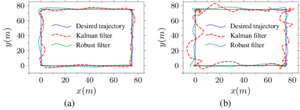
Figure 3: Panel (a) shows the trajectory tracking performance for the controller (IV) with the Kalman filter (dashed red line) and a robust filter (dotted green line) in nominal noise statistics (the desired trajectory is shown by the solid blue line). The controller with the Kalman filter outperforms the other. Panel (b) shows the tracking performance for the two controllers using non-nominal noise statistics. In non-nominal conditions, the controller with the Kalman filter performs worse than the controller with the robust filter. The performance of a controller is measured based on the mean squared deviation between the controlled and nominal trajectories (see also Fig. 4).

The statistics of the measurement noise in (26) depend on how the perception map is trained and the data samples used for the training. We aim to show that, if the estimator’s gain in (IV) is designed to minimize the estimation error based on the learned noise statistics, then the performance of the perception-based controller (IV) degrades significantly if the learned statistics differ from the actual noise statistics. Conversely, if the estimator’s gain in (IV) is designed based on Remark 2, then the performance of the perception-based controller (IV) remains robust across different values of the noise statistics, although lower than the performance of the optimal estimator operating with the nominal noise statistics. Fig. 3 shows the trajectory tracking performance for the controller (IV) for the Kalman filter and a robust filter with $T_{s}=1,Q=0.1I_{4},R=0.1I_{2},W_{x}=\text{diag}(100,10^{-3},100,10^{-3}),W_{u}=10^{-3}I_{2}$. The robust filter corresponds to $\lambda=0.307$ (see (14)). The non-nominal covariance is $\bar{R}=2.5I_{2}$. We observe that the controller based on the Kalman filter performs better in nominal conditions, while the controller based on the robust filter performs better in non-nominal conditions, as predicted by our theoretical results. Fig. 4 shows the error of the Kalman filter and the robust filter as a function of the changes of the measurement noise covariance. We notice that for small deviations (near-nominal conditions), the controller based on the Kalman filter performs better than the controller based on the robust filter. However, when the deviation of the noise statistics becomes substantially large, the controller based on the robust filter performs better, thereby validating our theoretical trade-off.

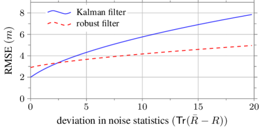
Figure 4: This figure shows the root mean square error (RMSE) of the controller (IV) with the Kalman filter (solid blue line) and the robust filter (dashed red line), as a function of deviation between the measurement noise statistics. For small deviations, the controller using the Kalman filter outperforms the other. For large deviations, the controller using the robust filter outperforms the controller using the Kalman filter.

As shown in Fig. 1(b), the perception error may not be normally distributed, especially in the case of non-nominal measurements. Although our theoretical results were obtained under the assumption that the measurement (perception) error is normally distributed, we next numerically show that a trade-off still exists when the measurement (perception) error is not Gaussian. To this aim, we consider the system in (24) and (26), where the measurement noise is distributed as in Fig. 1(b) (these distributions are computed numerically using the simulator CARLA [11]). We design $6$ estimators using (14) with different values of $\delta$, and test the performance of each estimator in nominal and non-nominal conditions. The performance of each estimator in nominal and non-nominal environments, denoted by $\mathcal{P}_{\text{nom}}$ and $\mathcal{P}_{\text{adv}}$, respectively, is computed using the sample error covariance computed from the obtained samples of the estimation error in nominal and non-nominal conditions. We approximate the sensitivity of these estimators as the relative degradation of the nominal performance when operating in non-nominal conditions, that is, as $(\mathcal{P}_{\text{adv}}-\mathcal{P}_{\text{nom}})/\mathcal{P}_{\text{nom}}$. Fig. 5 shows the performance and approximate sensitivity of the estimators. It can be seen that, even when the measurement error is not normally distributed, the estimator with largest (respectively, smallest) accuracy also has highest (respectively, smallest) sensitivity. These numerical results suggest that a tradeoff exists independently of the statistical properties of the measurement error.

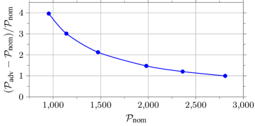
Figure 5: For the system (24) and (26) with measurement error distributed as in Fig. 1(b), this figure shows the performance $\mathcal{P}_{\text{nom}}$ (i.e., trace of estimation error covariance) and the approximate sensitivity $(\mathcal{P}_{\text{adv}}-\mathcal{P}_{\text{nom}})/\mathcal{P}_{\text{nom}}$ for $6$ different estimators obtained from (14) by varying the desired accuracy $\delta$. Although the measurement error is not normally distributed, a trade-off still emerges between the accuracy of the estimators and their sensitivity.

We conclude by showing that the identified trade-off between accuracy and robustness of linear estimators also constrain the performance of closed-loop perception-based control algorithms. To this aim, consider the system (24) with controller (IV), where both the estimator gain $K$ and the controller gain $L$ are now design parameters. For weighing matrices $W_{x}>0$ and $W_{u}>0$, let the performance of (IV) be

$$\mathcal{J}(K,L)=\mathbb{E}\Bigg{[}\frac{1}{T}\bigg{(}\sum_{t=0}^{T}x(t)^{\mathsf{T}}W_{x}x(t)+u(t)^{\mathsf{T}}W_{u}u(t)\bigg{)}\Bigg{]},$$ (28)

where $T$ denotes the time horizon. Notice that a lower value of the cost $J$ is desirable, and the minimum (for $T\rightarrow\infty$) is achieved by choosing the Kalman gain $K_{\text{kf}}$ with the linear quadratic regulator gain $L_{\text{lqr}}$ for the matrices $W_{x}$ and $W_{u}$. We adopt the following definition of sensitivity (this metric is the equivalent of (7) for the closed-loop performance):

$$\mathcal{S}_{\mathcal{J}}(K,L)\triangleq \mathsf{Tr}\Bigg{[}\frac{\partial\mathcal{J}(K,L)}{\partial R}\Bigg{]},$$ (29)

where $R$ is the noise covariance matrix of (26). To see if a trade-off exists beween performance and sensitivity of the closed-loop controller, we solve the following problem:

$$\mathcal{S}_{\mathcal{J}}^{*}(\delta)= \;\underset{K,L}{\min}\quad\mathcal{S}_{\mathcal{J}}(K,L)$$ (30)

$$\;\text{s.t.}\quad\mathcal{J}(K,L)\leq\delta,$$

where $\delta$ is a constant satisfying $\delta\geq\mathcal{J}(K_{\text{kf}},L_{\text{lqr}})$. Notice that the minimization problem (30) is similar to (8) for the considered closed-loop control setting. The results of the minimization problem (30) are reported in Fig. 6, where it can be seen that a trade-off between the performance of the controller (IV) and its sensitivity still exists. Interestingly, our numerical results show that the trade-off curve can be obtained, equivalently, by optimizing over both the controller and the estimator gain, by fixing the controller gain to be the LQR gain and optimizing over the estimator gain, or by fixing the estimator gain to be the Kalman gain and optimizing over the controller gain. Further, if the controller gain is chosen to be the optimal LQR gain, then the estimator gain that solves (30) coincides with the estimator gain obtained in Theorem III.3. We leave a formal characterization of these properties as the subject of future investigation.

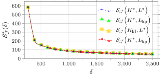
Figure 6: This figure shows the accuracy versus robustness trade-off in the closed loop setting described in Section IV. The blue, green, and yellow lines denote the solution of (30), where in the blue line we optimize over both gains, in the green line we fix the controller to the LQR gain and optimize over the estimator only, and in the yellow line we fix the estimator to the Kalman gain and optimize over the controller only. The red line denotes the trade-off between the accuracy in (28) and the sensitivity in (29) with the estimator gain given in (14) and the controller fixed to the LQR gain.

V Conclusion and future work

In this paper we show that a fundamental trade-off exists between the accuracy of linear estimation algorithms and their robustness to unknown changes of the measurement noise statistics. Because of this trade-off, estimators that are optimal with nominal sensing data may perform poorly in practice due to variations of the measurements statistics or different operational conditions. Conversely, robust estimators obtained through a more detailed design process may maintain similar performance levels in nominal and non-nominal conditions, but considerably underperform in nominal conditions when compared to nominally optimal estimators. To complement these results, we characterize the structure of optimal estimators, for desired levels of accuracy and robustness, and show that the trade-off also constrain the performance of closed-loop perception-based controllers.

The results in this paper complement a recent line of research aimed at deriving provable guarantees and performance limitations of machine learning and data-driven algorithms [1, 2, 3, 4], and extend such results, for the first time, to an estimation and control setting. This research area contains several timely and challenging open problems, including an explicit quantification of the performance of data-driven control algorithms when data is scarce and corrupted, and the design of provably robust data-driven control algorithms.

References

- [1] A. A. A. Makdah, V. Katewa, and F. Pasqualetti. A fundamental performance limitation for adversarial classification. IEEE Control Systems Letters, 4(1):169–174, 2019.
- [2] D. Tsipras, S. Santurkar, L. Engstrom, A. Turner, and A. Madry. Robustness may be at odds with accuracy. In International Conference on Learning Representations, Ernest N. Morial Convention Center, NO, USA, May 2019.
- [3] Z. Deng, C. Dwork, J. Wang, and Y. Zhao. Architecture selection via the trade-off between accuracy and robustness. arXiv preprint arXiv:1906.01354, 2019.
- [4] H. Zhang, Y. Yu, J. Jiao, E. Xing, L. E. Ghaoui, and M. I. Jordan. Theoretically principled trade-off between robustness and accuracy. In International Conference on Machine Learning, volume 97 of Proceedings of Machine Learning Research, pages 7472–7482, Long Beach, California, USA, Jun 2019. PMLR.
- [5] B. Recht. A tour of reinforcement learning: The view from continuous control. Annual Review of Control, Robotics, and Autonomous Systems, 2018.
- [6] F. L. Lewis, D. Vrabie, and K. G. Vamvoudakis. Reinforcement learning and feedback control: Using natural decision methods to design optimal adaptive controllers. IEEE Control Systems Magazine, 32(6):76–105, 2012.
- [7] P. Zhu, J. Isaacs, B. Fu, and S. Ferrari. Deep learning feature extraction for target recognition and classification in underwater sonar images. In IEEE Conference on Decision and Control, pages 2724–2731, Melbourne, Australia, Dec 2017.
- [8] S. Dean, N. Matni, B. Recht, and V. Ye. Robust guarantees for perception-based control. arXiv preprint arXiv:1907.03680, 2019.
- [9] S. Lohr. A lesson of Tesla crashes? Computer vision can’t do it all yet. The New York Times, Online, September 2016.
- [10] A. Ilyas, S. Santurkar, D. Tsipras, L. Engstrom, B. Tran, and A. Madry. Adversarial examples are not bugs, they are features. In Neural Information Processing Systems, pages 125–136, Vancouver Convention Center, Vancouver, Canada, Dec 2019. Curran Associates, Inc.
- [11] A. Dosovitskiy, G. Ros, F. Codevilla, A. Lopez, and V. Koltun. CARLA: An open urban driving simulator. In Conference on Robot Learning, volume 78 of Proceedings of Machine Learning Research, pages 1–16, Mountain View, CA, USA, Nov 2017. PMLR.
- [12] C. Szegedy, W. Zaremba, I. Sutskever, J. Bruna, D. Erhan, I. Goodfellow, and R. Fergus. Intriguing properties of neural networks. In International Conference on Learning Representations, Banff, Canada, Apr 2014.
- [13] I. J. Goodfellow, J. Shlens, and C. Szegedy. Explaining and harnessing adversarial examples. In International Conference on Learning Representations, San Diego, USA, May 2015.
- [14] S. Yasini and K. Pelckmans. Worst-case prediction performance analysis of the kalman filter. IEEE Transactions on Automatic Control, 63(6):1768–1775, June 2018.
- [15] B. Hassibi and T. Kaliath. bounds for least-squares estimators. IEEE Transactions on Automatic Control, 46(2):309–314, February 2001.
- [16] O. Anava, E. Hazan, and S. Mannor. Online learning for adversaries with memory: price of past mistakes. In Advances in Neural Information Processing Systems, pages 784–792, 2015.
- [17] K. Zhou and J. C. Doyle. Essentials of robust control, volume 104. Prentice Hall Upper Saddle River, NJ, 1998.
- [18] N. Madjarov and L. Mihaylova. Kalman filter sensitivity with respect to parametric noises uncertainty. Kybernetika, 32(3):307–322, 1996.
- [19] J. Kelly and G. S. Sukhatme. Visual-inertial sensor fusion: Localization, mapping and sensor-to-sensor self-calibration. International Journal of Robotics Research, 30(1):56–79, 2011.
- [20] G. Loianno, C. Brunner, G. McGrath, and V. Kumar. Estimation, control, and planning for aggressive flight with a small quadrotor with a single camera and imu. IEEE Robotics and Automation Letters, 2(2):404–411, 2016.
- [21] S. Bansal, V. Tolani, S. Gupta, J. Malik, and C. Tomlin. Combining optimal control and learning for visual navigation in novel environments. In Conference on Robot Learning, volume 100 of Proceedings of Machine Learning Research, Senri Life Science Center, Osaka, Japan, Nov 2019. PMLR.
- [22] T. Kailath. Linear Systems. Prentice-Hall, 1980.
- [23] F. Pasqualetti, F. Dörfler, and F. Bullo. Attack detection and identification in cyber-physical systems. IEEE Transactions on Automatic Control, 58(11):2715–2729, 2013.
- [24] B. Hassibi, A. H. Sayed, and T. Kailath. Indefinite-Quadratic Estimation and Control: A Unified Approach to H2 and H-infinity Theories, volume 16. SIAM, 1999.