Q-learning for POMDP: An application to learning locomotion gaits

Abstract

This paper presents a Q-learning framework for learning optimal locomotion gaits in robotic systems modeled as coupled rigid bodies. Inspired by prevalence of periodic gaits in bio-locomotion, an open loop periodic input is assumed to (say) affect a nominal gait. The learning problem is to learn a new (modified) gait by using only partial noisy measurements of the state. The objective of learning is to maximize a given reward modeled as an objective function in optimal control settings. The proposed control architecture has three main components: (i) Phase modeling of dynamics by a single phase variable; (ii) A coupled oscillator feedback particle filter to represent the posterior distribution of the phase conditioned in the sensory measurements; and (iii) A Q-learning algorithm to learn the approximate optimal control law. The architecture is illustrated with the aid of a planar two-body system. The performance of the learning is demonstrated in a simulation environment.

I INTRODUCTION

Biological locomotion is the movement of an animal from one location to another location, through periodic changes in the shape of the body, along with interaction with the environment [7]. The periodic motion of the shape, which constitutes the building block of locomotion, is called the locomotion gait. Examples of the locomotion gait are legged locomotion, flapping of the wings for flying, or wavelike motion of the fish for swimming. It is a wonderful example for learning because the dynamics are complicated but the goals (reward function) are easily modeled. In direct application of Q-learning to these problems, however, a problem arises because the full state is not available.

The dynamics for such robotic systems are modeled using coupled rigid bodies. The configuration space is split into two sets of variables: (i) the shape variable that describes the robot’s internal degrees of freedom; (ii) and the group variable that describes the global position and orientation of the robot. The dynamics of the shape variable is given by a second-order differential equation driven by control inputs. The dynamics of the group variable is given by a first-order differential equation governed by non-holonomic constraints in the system (e.g conversation laws or no slipping conditions).

A typical approach to design the locomotion gait is to search for a periodic orbit in the shape space that leads to a desired net change in the group variable. This idea of producing a net change through underlying periodic motion is known as mechanical rectification  [3, 11] and the net change in the group variable is called geometric phase [9, 10, 12]. The optimal gait is obtained by searching over a parameterized set of trajectories in the shape space to optimize a given optimization criteria  [2, 17, 26, 15, 18, 6]. The resulting control law is open-loop and can suffer from issues due to uncertainties in the environment, or disturbance which perturbs the trajectory away from the orbit.

The problem considered in this paper is to learn an approximate optimal gait given an open-loop periodic input. We do not assume any control over this input: for example, it may correspond to the nominal gait or it may be exerted from the environment. The presence of the periodic input creates a limit cycle in the high-dimensional configuration space. The control problem is to actuate some of the system parameters to learn new types of gaits.

For the purpose of learning, no knowledge of dynamic models is assumed. Furthermore, knowledge of full state is not assumed. At each time, one only has access to partial noisy measurements of the state. The proposed control architecture builds upon our prior work on phase estimation [22] and its use for optimal control of bio-locomotion [20]. As in [20], the control problem is modeled as an optimal control problem. Since full state feedback is not assumed, we are in the partially observed settings. The original contribution of this work is to extend our prior work to a reinforcement learning framework whereby new gaits can be learned by the robot only through the use of noisy measurements and observed rewards.

The proposed control architecture has three parts:

1. Phase modeling: Under the assumed periodic input, the shape trajectory is a limit cycle in the high-dimensional phase space. The main complexity reduction technique is to introduce a phase variable $\theta(t)\in[0,2\pi]$ to parametrize the low-dimensional periodic orbit. The inspiration comes from neuroscience where phase reduction is a popular technique to obtain reduced order model of neuronal dynamics [8, 4].

2. Coupled oscillator feedback particle filter: We construct a nonlinear filtering algorithm to approximate the posterior distribution of the phase variable $\theta(t)$, given time history of sensory measurements. The coupled oscillator feedback particle filter (FPF) is comprised of a system of $N$ coupled oscillators  [23, 21]. The empirical distribution of the oscillators is used to approximate the posterior distribution.

3. Reinforcement learning: The control problem is cast as a partially observed optimal control problem. The posterior distribution represents an information state for the problem. A Q-learning algorithm is proposed where the Q-function is approximated through a linear function approximation. The weights are learned by implementing a gradient descent algorithm to reduce the Bellman error [27, 25, 13].

The key component of the proposed architecture is the system of coupled oscillators that is used to both represent the posterior distribution (the belief state) and to learn the optimal control policy. This control system can be viewed as a central pattern generator (CPG) which integrates sensory information to learn closed-loop optimal control policies for bio-locomotion.

The proposed CPG control architecture is illustrated with the aid of a two-body planar system depicted in Fig. 1. An open-loop periodic torque is applied at the joint connecting the two links, which results in the body to oscillate in a periodic (but uncontrolled) manner. The control objective is to turn the head clockwise by actuating the length of the tail body. Although only a two-body system is considered in this paper, the proposed architecture can easily be generalized to coupled body models of snake-robots and swimming fish robots. This is the subject of ongoing work.

The remainder of this paper is organized as follows: The problem is formulated in Section II. The proposed solution is described in Section III. The numerical results appear in Section IV.

II Problem Formulation

II-A Modeling and dynamics

Consider a system of two planar rigid bodies, the head body $B_{1}$ and the tail body $B_{2}$, connected by a single degree of freedom pin joint as depicted in Figure 1. The configuration variables of the system are divided into two sets: i) the shape variable; ii) and the group variable. For the two-body system, the shape variable is the relative orientation between two bodies. It is denoted as the angle $x$. The group variable is the absolute orientation of the frame rigidly affixed to head body. It is denoted as the angle $q$.

There is no external force applied to the system, which means that the total angular momentum is conserved. The joint is assumed to be actuated by a motor with driven torque $\tau$. An open-loop periodic input is assumed for the torque actuation:

$$\tau(t)=\tau_{0}\sin(\omega_{0}t)$$ (1)

where $\omega_{0}$ is the frequency and $\tau_{0}$ is the amplitude. There is no control objective associated with this torque input, except to have the shape variable $x$ oscillate in a periodic manner.

It is assumed that there exists a control actuation that changes the length of the tail body $B_{2}$ according to

$$d(t)=(1+u(t))\bar{d}$$ (2)

where $\bar{d}$ is the nominal length and $u$ represents the control input.

The dynamics of the two-body system is described by a second-order ODE for the shape variable and a first-order ODE for the group variable:

$$\ddot{x}(t) =\tilde{g}(x(t),\dot{x}(t),\tau(t),u(t)),\quad(x(0),\dot{x}(0))=(x_{0},\dot{x}_{0})$$ (3a)

$$\dot{q}(t) =\tilde{f}(x(t),\dot{x}(t),u(t))$$ (3b)

The explicit form of the functions $\tilde{f}$ and $\tilde{g}$ and their derivations appear in [20]. In this paper, the explicit form of $\tilde{f}$ and $\tilde{g}$ are assumed unknown. Rather, the dynamic model is treated as a simulator (black-box) that is used to simulate the dynamics (3a)-(3b).

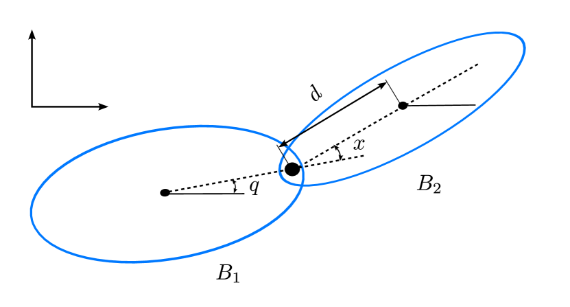
Figure 1: Schematic of the two-body system.

Remark 1

The modeling procedure is easily generalized to a chain of $n$ planar rigid links, e.g used to model snake robots as in [9]. In such systems, the group variable is the position and orientation of the robot, and the configuration space of shape variable is $n-1$ dimensional. With $n$ links, the dimension of the system is $2n+1$. An interesting problem for the snake robot is to learn a turning maneuver by changing the friction coefficients with respect to the surface.

II-B Observation process

For the purposes of learning and control design, the state $(x,\dot{x})$ is assumed to be unknown. The following continuous-time observation model is assumed for the sensor:

$$\,\mathrm{d}Z(t)=\tilde{h}(x(t),\dot{x}(t))\,\mathrm{d}t+\sigma_{W}\,\mathrm{d}W(t)$$ (4)

where $Z(t)\in\mathbb{R}$ denotes the observation at time $t$, $W(t)$ is a standard Wiener process, and $\sigma_{W}>0$ is the noise strength. The observation function $\tilde{h}:\mathbb{R}^{2}\to\mathbb{R}$ is known and is assumed to be $C^{1}$.

II-C Optimal control problem

The control objective is to turn the head body $B_{1}$ clockwise by actuating the control input $u(t)$. An uncontrolled periodic torque input (1) is assumed to be present. The control objective is modeled as a discounted infinite-horizon optimal control problem:

$$\tilde{J}(x_{0},\dot{x}_{0})=\underset{u(\cdot)}{\min}\ {\sf E}\left[\int_{0}^{\infty}e^{-\gamma t}\tilde{c}(x(t),\dot{x}(t),u(t))\,\mathrm{d}t\right]$$ (5)

subject to the dynamic constraints (3a). Here, $\gamma>0$ is the discount rate and the cost function

$$\tilde{c}(x,\dot{x},u)=\tilde{f}(x,\dot{x},u)+\frac{1}{2\epsilon}u^{2}$$

with $\epsilon>0$ as the control penalty parameter. The minimum is over all control inputs $u(\cdot)$ adapted to the filtration $\mathcal{Z}_{t}:=\sigma(Z(s);s\in[0,t])$ generated by the observation process.

The particular form of the cost function is assumed to maximize the rate of change, in the clockwise direction, in the group variable $q$. Indeed, by (3b), $\tilde{f}(x,\dot{x},u)=\dot{q}$. Therefore, minimizing the cost leads to net negative change in the head orientation $q(t)$. This corresponds to the clockwise rotation.

III Solution Approach

Solving the optimal control problem (5) is challenging because of the following reasons:

1. The function $\tilde{g}$ in the dynamic model (3a) is not known. For coupled rigid bodies, the model is nonlinear and complicated due to the details of the geometry, models of contact forces with the environment, uncertain parameters, etc.

2. The problem is partially observed, i.e., the state $(x,\dot{x})$ is not known. As the number of links grow, the state can be very high dimensional.

3. The explicit form of the function $\tilde{f}$ which captures the relationship between shape and group dynamics is not known.

These challenges are tackled by the following three-step procedure:

III-A Step 1. Phase modeling

Consider the second-order equation (3a) for the shape variable $x$ under the open-loop periodic input $\tau(t)$ given by (1). The following assumption is made concerning its solution:

• Under periodic forcing $\tau(t)$ as in (1), the solution to (3a) is given by an isolated asymptotically stable periodic orbit (limit cycle) with period ${2\pi}/{\omega_{0}}$.

Denote the set of points on limit cycle as $\mathcal{P}\subset\mathbb{R}^{2}$. The limit cycle solution is parameterized by a phase coordinate $\theta\in[0,2\pi)$ in the sense that there exists an invertible map $X_{LC}:[0,2\pi)\to\mathcal{P}$ such that $X_{\text{LC}}(\theta(t))=(x(t),\dot{x}(t))$, where $\theta(t)=(\omega_{0}t+\theta(0))$ mod $2\pi$ (see Figure 2). The definition of the phase variable is extended locally in a small neighborhood of the limit cycle by using the notion of isochrons [8].

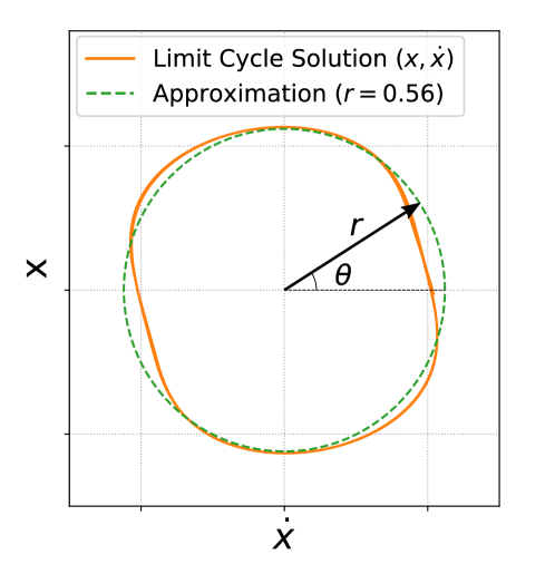
Figure 2: The limit cycle solution for the shape dynamics $(x(t),\dot{x}(t))$ together with its limit cycle approximation (see (21)).

In terms of the phase variable, the first-order dynamics of the group variable (3b) is expressed as

$$\dot{q}(t)=\tilde{f}(X_{LC}(\theta(t)),u(t))=:f(\theta(t),u(t))$$ (6)

and the observation model (4) is expressed as

$$\,\mathrm{d}Z(t)=h(\theta(t))\,\mathrm{d}t+\sigma_{W}\,\mathrm{d}W(t)$$ (7)

where $h(\theta):=\tilde{h}(X_{LC}(\theta))$.

The optimal control problem (5) in terms of the phase variable is given by

$$J(\theta_{0})=\underset{u(\cdot)}{\min}\ {\sf E}\left[\int_{0}^{\infty}e^{-\gamma t}c(\theta(t),u(t))\,\mathrm{d}t\right]$$ (8)

where $c(\theta,u)=f(\theta,u)+\frac{1}{2\epsilon}u^{2}$ and the minimum is over all control inputs $u(\cdot)$ adapted to the filtration $\mathcal{Z}_{t}$.

In contrast to the original problem, the new problem is described by a single phase variable. With $u(t)\equiv 0$, the dynamics is described by the oscillator model $\theta(t)=(\omega_{0}t+\theta_{0})$ mod $2\pi$. Now, in the presence of (small) control input, the dynamics need to be augmented by additional terms due to control:

$$\,\mathrm{d}\theta(t)=(\omega_{0}+\epsilon g(\theta(t)),u(t))\,\mathrm{d}t$$ (9)

III-B Step 2. Feedback particle filter (FPF)

A feedback particle filter is constructed to obtain the posterior distribution of the phase variable $\theta(t)$ given the noisy observations  (7). The filter is comprised of $N$ stochastic processes $\{\theta^{i}(t):1\leq i\leq N\}$, where the value $\theta^{i}(t)\in[0,2\pi]$ is the state of the $i$-th particle (oscillator) at time $t$. The dynamics evolves according to

$$\,\mathrm{d}\theta^{i}(t) =\omega^{i}\,\mathrm{d}t+\epsilon g(\theta^{i}(t)),u(t))\,\mathrm{d}t$$

$$\quad+\frac{{\sf K}(\theta^{i}(t),t)}{\sigma_{W}^{2}}\circ\left(\,\mathrm{d}Z(t)-\frac{h(\theta^{i}(t))+\hat{h}(t)}{2}\,\mathrm{d}t\right)$$ (10)

where $\omega^{i}\sim\text{Unif}([\omega_{0}-\delta,\omega_{0}+\delta])$ is the frequency of the $i$-th oscillator, the initial condition $\theta^{i}(0)=\theta^{i}_{0}\sim\text{Unif}([0,2\pi])$, and $\hat{h}(t):={\sf E}[h(\theta^{i}(t))|\mathcal{Z}_{t}]$. The notation $\circ$ denotes Stratonovich integration. In the numerical implementation, $\hat{h}(t)\approx N^{-1}\sum_{i=1}^{N}h(\theta^{i}(t))$.

Based on the FPF theory, the gain function ${\sf K}(\theta,t)$ is the solution of the Poisson equation, expressed in the weak-form as

$${\sf E}[{\sf K}(\theta(t),t)\psi^{\prime}(\theta_{t})|{\cal Z}_{t}]={\sf E}[(h(\theta_{t})-\hat{h})\psi(\theta(t))|{\cal Z}_{t}]$$ (11)

for all test functions $\psi$ where $\psi^{\prime}$ is the derivative. In the numerical implementation, the gain function is approximated by choosing $\psi$ from the Fourier basis functions $\{\sin(\theta),\cos(\theta)\}$ and approximating the expectations with empirical distribution of the oscillators $\{\theta^{i}(t):1\leq i\leq N\}$. The detailed numerical algorithm to approximate the gain function appears in  [23].

Remark 2

There are two manners in which control input $u(t)$ affects the dynamics of the filter state $\theta^{i}(t)$:

1. The $O(\epsilon)$ term $\epsilon g(\cdot,u(t))$ which models the effect of dynamics;

2. The FPF update term which models the effect of sensor measurements. This is because the control input $u(t)$ affects the state $x(t)$ (see (3a)) which in turn affects the sensor measurements $Z(t)$ (see (4)).

III-C Step 3. Q-learning

Using the FPF, following the approach presented in [14], express the partially observed optimal control problem (8) as a fully observed optimal control problem in terms of oscillator states $\theta^{(N)}(t)=(\theta^{1}(t),\ldots,\theta^{N}(t))$ according to

$$J^{(N)}(\theta^{(N)}_{0})=\underset{u(\cdot)}{\min}\ {\sf E}\left[\int_{0}^{\infty}e^{-\gamma t}c^{(N)}(\theta^{(N)}(t),u(t))\,\mathrm{d}t\right]$$ (12)

subject to (10), where the cost $c^{(N)}(\theta^{(N)},u):=\frac{1}{N}\sum_{i=1}^{N}c(\theta^{i},u)$ and the minimization is over all control laws adapted to the filtration $\mathcal{X}_{t}:=\{\theta^{i}(s);~{}s\leq t,1\leq i\leq N\}$. The problem is now fully observed because the states of oscillators $\theta^{(N)}(t)$ are known.

The analogue of the Q-function for continuous-time systems is the Hamiltonian function:

$$H^{(N)}(\theta^{(N)},u)=c^{(N)}(\theta^{(N)},u)+\mathcal{D}_{u}J^{(N)}(\theta^{(N)})$$ (13)

where $\mathcal{D}_{u}$ is the generator for (10) defined such that $\frac{\,\mathrm{d}}{\,\mathrm{d}t}{\sf E}[J^{(N)}(\theta^{(N)}(t))]=\mathcal{D}_{u}J^{(N)}(\theta^{(N)}(t))$.

The dynamic programming principle for the discounted problem implies:

$$\min_{u}~{}H^{(N)}(\theta^{(N)},u)=\gamma J^{(N)}(\theta^{(N)})$$ (14)

Substituting this into the definition of the Hamiltonian (13) yields the fixed-point equation:

$$\mathcal{D}_{u}~{}\underline{H}^{(N)}(\theta^{(N)})=\gamma(c^{(N)}(\theta^{(N)},u)-H^{(N)}(\theta^{(N)},u))$$ (15)

where $\underline{H}^{(N)}(\theta^{(N)}):=\min_{u}~{}H^{(N)}(\theta^{(N)},u)$. This is the fixed-point equation that appears in the Q-learning.

Linear function approximation: Learning the exact Hamiltonian (Q-function) is an infinite-dimensional problem. Therefore, we set the goal to learn an approximation. For this purpose, consider a fixed set of $M$ real-valued functions $\{\phi^{(m)}(\theta,u)\}_{m=1}^{M}$. The Hamiltonian is approximated as the linear combination of the basis functions as follows:

$$\hat{H}^{(N)}(\theta^{(N)},u;w) =\frac{1}{N}\sum_{i=1}^{N}w^{T}\phi(\theta^{i},u)$$ (16)

where $w\in\mathbb{R}^{M}$ is a vector of parameters (or weights) and $\phi=(\phi^{(1)},\phi^{(2)},\ldots,\phi^{(M)})^{T}$ is a vector of basis functions. Thus, the infinite-dimensional problem of learning the Hamiltonian function is converted into the problem of learning the $M$-dimensional weight vector $w$.

Define the point-wise Bellman error according to

$$\mathcal{E}(\theta^{(N)},u;w):= \mathcal{D}_{u}\hat{\underline{H}}^{(N)}(\theta^{(N)};w)$$ (17)

$$+\gamma(c^{(N)}(\theta^{(N)},u)-\hat{H}^{(N)}(\theta^{(N)},u;w))$$

where $\hat{\underline{H}}^{(N)}(\theta^{(N)};w):=\min_{u}~{}\hat{H}^{(N)}(\theta^{(N)},u;w)$.

The following learning algorithm is proposed to find the optimal parameters

$$\frac{\,\mathrm{d}}{\,\mathrm{d}t}w(t)=-\frac{1}{2}\alpha(t)\nabla_{w}\mathcal{E}^{2}(\theta^{(N)}(t),u(t);w(t))$$ (18)

where $\alpha(t)$ is the time-varying learning gain and $u(t)$ is chosen to explore the state-action space. For convergence analysis of the Q-learning algorithm see [24, 19, 5, 16].

Given a learned weight vector $w^{*}$, the learned optimal control policy is given by:

$$\hat{u}^{*}(\theta^{(N)};w^{*})=\underset{v}{\arg\min}\ \hat{H}^{(N)}(\theta^{(N)},v;w^{*})$$ (19)

III-D Information structure

In order to implement the algorithm, one requires knowledge of the following models:

1. A model for $g(\theta,u)$ which represents the reduced order model of dynamics as these affect the phase variable;

2. A model for $h(\theta)$ which represents the reduced order model of the sensor.

These models are needed to implement the coupled oscillator FPF (10). It is noted that both the models are described with respect to the phase variable $\theta$.

In the simulation results presented next, we assume knowledge of $h(\theta)$ and ignore the term $\epsilon g(\theta^{i}(t),u(t))$ in the FPF. The formal reason for ignoring the term is that it is small ($O(\epsilon)$) compared to other terms, $O(1)$ frequency $\omega_{0}$ and the update term. Although, we assume knowledge of the sensor model $h(\theta)$ for this paper, a learning algorithm could also be implemented to learn the sensor model in an online manner. This is the subject of future work.

In numerical implementation, the generator $\mathcal{D}_{u}$ is approximated as

$$\mathcal{D}_{u}\hat{\underline{H}}^{(N)}(\theta^{(N)}(t))\approx\frac{\hat{\underline{H}}^{(N)}(\theta^{(N)}(t+\Delta t))-\hat{\underline{H}}^{(N)}(\theta^{(N)}(t))}{\Delta t}$$

where $\Delta t$ is the discrete time step-size in the numerical algorithm and $\{\theta^{i}(t)\}_{i=1}^{N}$ is the state of the oscillators at time $t$.

The reward function $f(\theta(t),u(t))$ in the cost function is approximated as

$$f(\theta(t),u(t))=\dot{q}(t)\approx\frac{q(t+\Delta t)-q(t)}{\Delta t}$$

where $q(t)$ is available through the (black-box) simulator.

The overall algorithm appears in Table 1.

Algorithm 1 Q-learning for Optimal Contol of Two-body System

1:Parameters in Table I and a simulator for (3a)-(3b)-(4)

2:Optimal control policy $\hat{u}^{*}(\theta^{(N)};w)$.

3:Initialize particles $\{\theta_{0}^{i}\}_{i=1}^{N}\sim\text{Unif}([0,2\pi])$;

4:Initialize weight vector $w_{0}$ according to (22).

5:for $k=0$ to $t_{T}/\Delta t-1$ do

6:     Choose control input $u_{k}$ according to (23);

7:     Input $u_{k}$ to the simulator and output $Z_{k}$ and $q_{k}$

8:     Update particles in FPF

$$\theta_{k+1}^{i}=\theta_{k}^{i}+\omega^{i}\Delta t+\frac{{\sf K}(\theta_{k}^{i})}{\sigma_{W}^{2}}(Z_{k+1}-Z_{k}-\frac{h(\theta_{k}^{i})+\hat{h}_{k}}{2}\Delta t)$$

9:     Compute the cost $c_{k}=\frac{1}{\Delta t}(q_{k+1}-q_{k})+\frac{1}{2\epsilon}u_{k}^{2}$

10:     Compute

$$\mathcal{D}_{u}\hat{\underline{H}}^{(N)}_{k}=\frac{1}{\Delta t}(\hat{\underline{H}}^{(N)}(\theta^{(N)}_{k+1};w_{k})-\hat{\underline{H}}^{(N)}(\theta^{(N)}_{k};w_{k}))$$

11:     Compute Bellman error

$$\mathcal{E}_{k}=\mathcal{D}_{u}\hat{\underline{H}}^{(N)}_{k}+\gamma(c_{k}-\hat{H}^{(N)}(\theta^{(N)}_{k},u_{k};w_{k}))$$

12:     Update weight vector $w_{k+1}=w_{k}-\Delta t\alpha_{k}\mathcal{E}_{k}\nabla_{w}\mathcal{E}_{k}$

13:end for

14:Output the learned control policy $\hat{u}^{*}(\theta^{(N)};w_{k})$ from (19).

III-E Approximate formula for optimal control input

Assuming the knowledge of the explicit form of the function $f(\theta,u)$, a semi-analytic approach is presented in [20] to derive the following approximate formula for optimal control:

$$u^{*}(t)\approx\frac{\epsilon C}{N}\sum_{i=1}^{N}\cos(\theta^{i}(t))$$ (20)

where $C$ is a constant that depends on the parameters of the model. The formula was shown to be valid in the asymptotic limit as $\epsilon\to 0$. The control policy (20) is implemented in [20] where it is numerically shown to lead to clockwise rotation of the head body.

The formula (20) serves as a baseline for comparison with the results of the numerical implementation of the Q-learning algorithm.

IV Numerics

TABLE I: Parameters for Numerical Simulation

Parameter	Description	Numerical value
Two-body system
$m_{i}$	Mass of body $B_{i}$	$m_{1}=1$	$m_{2}=\frac{1}{2}$
$I_{i}$	Moment of inertia of body $B_{i}$	$I_{1}=\frac{2}{3}$	$I_{2}=\frac{1}{6}$
$d_{i}$	Span of body $B_{i}$	$d_{1}=1$	$d_{2}=1$
Some auxiliary parameters
$\tilde{m}=\frac{m_{1}m_{2}}{m_{1}+m_{2}},\quad\tilde{I}_{i}=I_{i}+\tilde{m}d_{i}^{2},\quad\lambda=\tilde{m}d_{1}d_{2}$
$A_{i}(x)=\tilde{I}_{i}+\lambda\cos(x),\quad\Delta(x)=\tilde{I}_{1}\tilde{I}_{2}-\lambda^{2}\cos^{2}(x)$
Dynamic model
$\omega_{0}$	Input torque frequency	$1.0$
$\tau_{0}$	Input torque amplitude	$1.0$
$\kappa$	Torsional spring coefficient	$2.0$
$b$	Viscous friction coefficient	$0.1$
Sensor & FPF
$\Delta t$	Discrete time step-size	$0.01$
$\sigma_{W}$	Noise process std. dev.	$0.1$
$N$	Number of particles	$1000$
$\delta$	Heterogeneous parameter	$0.12$
Q-learning
$t_{T}$	simulation terminal time	$100\text{\textperiodcentered}2\pi\text{/}\omega_{0}$
$\gamma$	Discount rate	$1.0$
$\epsilon$	Control penalty parameter	$1.0$
$\alpha_{k}$	Learning gain	$0.5$
$A$	Control exploration amplitude	$0.25$

In this section, we present the numerical results. These results illustrate the i) phase modeling; ii) the performance of coupled oscillator FPF; and iii) the performance of Q-learning algorithm. The numerical results are based on the use of Algorithm 1. The simulation parameters are tabulated in Table I.

IV-A Simulator

The simulator takes the control input $u(t)$ and outputs the shape variable $x(t)$, the head orientation $q(t)$, and the observation $Z(t)$ according to (3a), (3b), and (4) respectively. The explicit form of the simulated dynamics (3a)-(3b) are as follows:

$$\ddot{x} =\frac{1}{\Delta}\left[-\lambda\sin(x)\frac{A_{1}A_{2}}{A_{1}+A_{2}}\dot{x}^{2}+(A_{1}+A_{2})(\tau(t)-\kappa x-b\dot{x})\right]$$

$$\dot{q} =\frac{\tilde{I}_{2}+\lambda\cos(x)}{\tilde{I}_{1}+\tilde{I}_{2}+2\lambda\cos(x)}\dot{x}$$

where the parameters are defined in Table I; cf., [20] for additional details on modeling. The resulting state trajectory $x(t)$ and head orientation $q(t)$, under periodic open-loop torque $\tau(t)$ (see (1)), are depicted in Figure 3. It is observed that without control input, the head orientation oscillates, without any net change.

The observation signal $y(t):=(Z(t+\Delta t)-Z(t))/\Delta t$, with the step-size $\Delta t=0.01$ is depicted in Figure 3. The observation model is taken as $\tilde{h}(x,\dot{x})=x$. The noise strength $\sigma_{w}=0.1$.

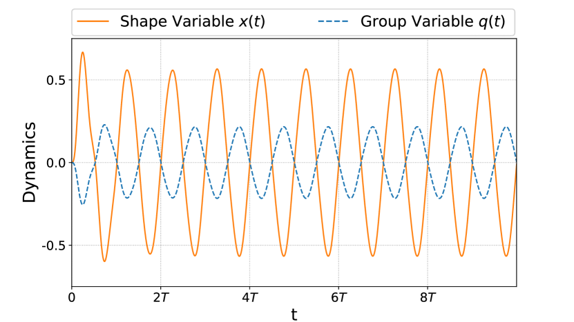
Figure 3: Summary of numerical results for the two-body system simulator: (a) Trajectory for the shape variable $x(t)$ and the the head orientation $q(t)$ under no control input ($u(t)\equiv 0$); (b) Observation process $y(t)$.

IV-B Phase modeling

The limit cycle solution for the shape dynamics (3a) is depicted in Figure 2. The map $\tilde{X}_{LC}(\theta(t))=(x(t),\dot{x}(t))$ is approximated as

$$\tilde{X}_{LC}(\theta) \approx(r\sin(\theta),r\omega_{0}\cos(\theta))$$ (21)

where $r=0.56$ is numerically determined.

IV-C Coupled oscillator feedback particle filter

The trajectories of $N=1000$ particles in the FPF algorithm (10) are depicted in Figure 4. The initial conditions $\theta_{0}^{i}$ are drawn from a uniform distribution in $[0,2\pi]$. The initial transients due to the initial condition converge rapidly. The true phase variable $\theta(t)$ is also depicted as a solid line. It is observed that the ensemble of particles synchronize and track the true phase.

The true state $(x(t),\dot{x}(t))$, along with the empirical distribution of the particles, at two time instants, are shown in Figure 4. The particles are positioned on the approximate limit cycle map (21). These results show that the filter is able to track the true state on the limit cycle accurately.

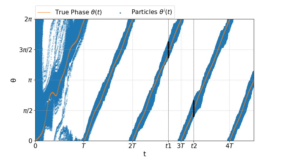
Figure 4: Summary of estimation results: (a) Time trace of $N=1000$ particles in the FPF algorithm compared with the true phase $\theta(t)$; (b) Empirical distribution of the particles compared with the true state $(x,\dot{x})$ at two time instants $t_{1}$ and $t_{2}$.

IV-D Q-learning

To approximate the Hamiltonian function in (16), the basis functions are selected to be the product of Fourier basis functions of $\theta$ and polynomial functions of $u$ as follows:

$$\phi(\theta,u)=\big{(} \cos(\theta),\sin(\theta),\cos(2\theta),\sin(2\theta),$$

$$u\cos(\theta),u\sin(\theta),u\cos(2\theta),u\sin(2\theta),\frac{1}{2}u^{2}\big{)}^{T}$$

The weight vector $w_{0}=\Big{(}w_{0}^{(1)},...,w_{0}^{(9)}\Big{)}^{T}$ is initialized randomly as follows:

$$w_{0}^{(m)} \sim\text{Unif}([-1,1])\quad\text{for }m=1,\ldots,8$$ (22)

$$w_{0}^{(9)} \sim\text{Unif}([0.9,1.1])$$

The reason for choosing the particular initialization for $w_{0}^{(9)}$is to avoid numerical issues due to large control values whenever $w_{0}^{(9)}$ is small.

The exploration control input $u(t)$ to be used in (18) is chosen as a combination of sinusoidal functions with irrationally related frequencies as follows:

$$u(t)=A\sin(\omega_{0}t)+A\sin(\pi\omega_{0}t)$$ (23)

The rationale for doing so is to explore the state-action space [1].

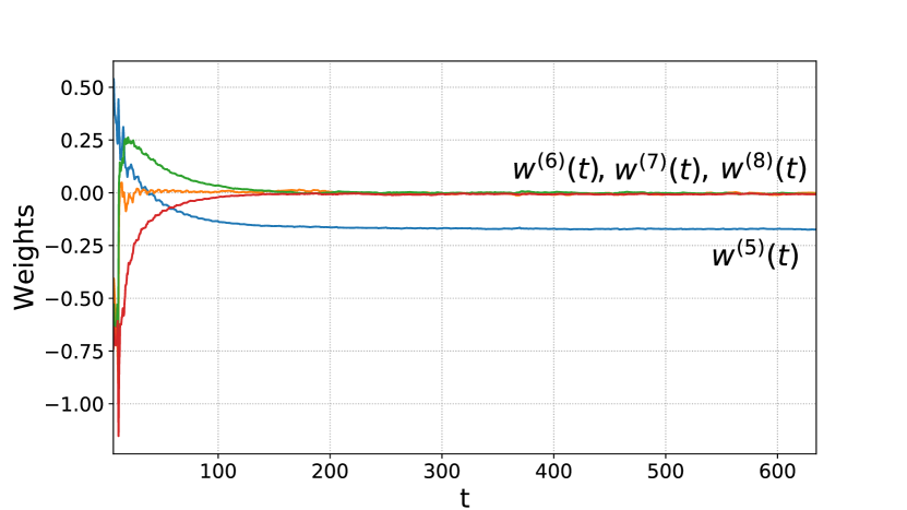
Figure 5: Summary of Q-learning results: (a) The Bellman error as a function of time; (b) Convergence of the four weight components in the learned optimal control law (25).

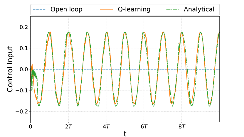
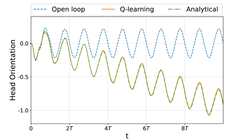
Figure 6: Summary of control results: (a) Comparison of the control input learned from Q-learning (25) and the semi-analytical optimal control input (20); (b) Time trace of the orientation with no control input ($u(t)\equiv 0$), semi-analytical control input, and the learned control input.

The $L^{2}$-norm of the point-wise Bellman error (17), over the $j$-th period is denoted as $e_{j}$ and defined to be:

$$e_{j}:=\frac{1}{T}\int_{(j-1)T}^{jT}\Big{|}\mathcal{E}(\theta^{(N)}(t),u(t);w(t))\Big{|}^{2}\,\mathrm{d}t$$ (24)

The average of the error $e_{j}$ and its variance over fifty Monte-Carlo runs are depicted in Figure 5. It is observed that the Bellman error drops by over three orders of magnitude. This suggests that the algorithm is able to learn the Hamiltonian function that solves the dynamic programming fixed-point equation (15).

The learned optimal control policy (19) in terms of the selected basis functions is given by:

$$\hat{u}^{*}(\theta^{(N)};w)= -\frac{1}{N}\sum_{i=1}^{N}\left(\frac{w^{(5)}}{w^{(9)}}\cos(\theta^{i})+\frac{w^{(6)}}{w^{(9)}}\sin(\theta^{i})\right)$$ (25)

$$-\frac{1}{N}\sum_{i=1}^{N}\left(\frac{w^{(7)}}{w^{(9)}}\cos(2\theta^{i})+\frac{w^{(8)}}{w^{(9)}}\sin(2\theta^{i})\right)$$

The traces of the four components of the weight vector $\{w^{(5)}(t),w^{(6)}(t),w^{(7)}(t),w^{(8)}(t)\}$ are depicted in Figure 5. It is observed that the components (weights) converge quickly. Also, the component $w^{(5)}(t)$, which corresponds to $\cos(\cdot)$, dominates while other components converge to zero.

Figure 6 depicts the learned optimal control policy as a function of time. Also depicted is a comparison with the semi-analytical solution (20). It is observed that the learned optimal control coincides with the analytical formula in terms of both phase and amplitude.

Figure 6 depicts the resulting head orientation with i) the learned optimal control policy (25); ii) the analytical control law (20); and iii) with no control input ($u(t)\equiv 0$). It is observed that the learned optimal control input induces nearly the same net change in the head orientation as the analytical control law. That is, the Q-learning algorithm is able to learn the optimal control policy to rotate the head body clockwise.

.

V Conclusions and Future Work

We introduced a coupled oscillator-based framework for learning the optimal control of periodic locomotory gaits. The framework does not require knowledge of the explicit form of the dynamic models or observation of the full state. The framework was illustrated on the problem of turning the two-body planar system. One direction for future work, is to apply the framework to more complicated models such as coupled kinematic chains and continuum models. Another direction of future work is to consider more advanced tasks such as turning to a certain angle or locating a target.

References

- [1] D. P. Bertsekas and J. N. Tsitsiklis. Neuro-dynamic programming, volume 5. Athena Scientific Belmont, MA, 1996.
- [2] J. Blair and T. Iwasaki. Optimal gaits for mechanical rectifier systems. IEEE Transactions on Automatic Control, 56(1):59–71, 2011.
- [3] R. W. Brockett. Pattern generation and the control of nonlinear systems. IEEE transactions on automatic control, 48(10):1699–1711, 2003.
- [4] E. Brown, J. Moehlis, and P. Holmes. On the phase reduction and response dynamics of neural oscillator populations. Neural computation, 16(4):673–715, 2004.
- [5] E. Even-Dar and Y. Mansour. Learning rates for q-learning. Journal of Machine Learning Research, 5(Dec):1–25, 2003.
- [6] R. L. Hatton and H. Choset. Generating gaits for snake robots: annealed chain fitting and keyframe wave extraction. Autonomous Robots, 28(3):271–281, 2010.
- [7] P. Holmes, R. J. Full, D. Koditschek, and J. Guckenheimer. The dynamics of legged locomotion: Models, analyses, and challenges. SIAM review, 48(2):207–304, 2006.
- [8] E. M Izhikevich. Dynamical systems in neuroscience. MIT press, 2007.
- [9] S. D. Kelly and R. M. Murray. Geometric phases and robotic locomotion. Journal of Robotic Systems, 12(6):417–431, 1995.
- [10] P. S. Krishnaprasad. Geometric phases, and optimal reconfiguration for multibody systems. In 1990 American Control Conference, pages 2440–2444. IEEE, 1990.
- [11] P. S. Krishnaprasad. Motion control and coupled oscillators. In Proc. Symposium on Motion, Control, and Geometry, 1997.
- [12] J. E. Marsden, R. Montgomery, and T. S. Ratiu. Reduction, symmetry, and phases in mechanics, volume 436. American Mathematical Soc., 1990.
- [13] P. G. Mehta and S. P. Meyn. Q-learning and pontryagin’s minimum principle. In Proceedings of the 48h IEEE Conference on Decision and Control (CDC) held jointly with 2009 28th Chinese Control Conference, pages 3598–3605. IEEE, 2009.
- [14] P. G. Mehta and S. P. Meyn. A feedback particle filter-based approach to optimal control with partial observations. In 52nd IEEE conference on decision and control, pages 3121–3127. IEEE, 2013.
- [15] J. B Melli, C. W. Rowley, and D. S. Rufat. Motion planning for an articulated body in a perfect planar fluid. SIAM Journal on applied dynamical systems, 5(4):650–669, 2006.
- [16] E. Moulines and F. R. Bach. Non-asymptotic analysis of stochastic approximation algorithms for machine learning. In Advances in Neural Information Processing Systems, pages 451–459, 2011.
- [17] R. M. Murray and S. S. Sastry. Nonholonomic motion planning: Steering using sinusoids. IEEE transactions on Automatic Control, 38(5):700–716, 1993.
- [18] J. Ostrowski, A. Lewis, R. Murray, and J. Burdick. Nonholonomic mechanics and locomotion: the snakeboard example. In Proceedings of the 1994 IEEE International Conference on Robotics and Automation, pages 2391–2397. IEEE, 1994.
- [19] C. Szepesvári. The asymptotic convergence-rate of q-learning. In Advances in Neural Information Processing Systems, pages 1064–1070, 1998.
- [20] A. Taghvaei, S. A. Hutchinson, and P. G. Mehta. A coupled oscillators-based control architecture for locomotory gaits. In Decision and Control (CDC), 2014 IEEE 53rd Annual Conference on, pages 3487–3492. IEEE, 2014.
- [21] A. K. Tilton, E. T. Hsiao-Wecksler, and P. G. Mehta. Filtering with rhythms: Application to estimation of gait cycle. In 2012 American Control Conference (ACC), pages 3433–3438. IEEE, 2012.
- [22] A. K. Tilton and P. G. Mehta. Control with rhythms: A cpg architecture for pumping a swing. In American Control Conference (ACC), 2014, pages 584–589. IEEE, 2014.
- [23] A. K. Tilton, P. G. Mehta, and S. P. Meyn. Multi-dimensional feedback particle filter for coupled oscillators. In 2013 American Control Conference, pages 2415–2421. IEEE, 2013.
- [24] J. N. Tsitsiklis and B. Van Roy. Optimal stopping of markov processes: Hilbert space theory, approximation algorithms, and an application to pricing high-dimensional financial derivatives. IEEE Transactions on Automatic Control, 44(10):1840–1851, 1999.
- [25] D. Vrabie, M. Abu-Khalaf, F. L. Lewis, and Y. Wang. Continuous-time adp for linear systems with partially unknown dynamics. In 2007 IEEE International Symposium on Approximate Dynamic Programming and Reinforcement Learning, pages 247–253. IEEE, 2007.
- [26] G. C. Walsh and S. S. Sastry. On reorienting linked rigid bodies using internal motions. IEEE Transactions on Robotics and Automation, 11(1):139–146, 1995.
- [27] C. J. C. H. Watkins. Learning from delayed rewards. PhD thesis, King’s College, Cambridge, 1989.