Highly frustrated magnetism in relativistic $\boldsymbol{d}^{\mathbf{4}}$ Mott insulators:
Bosonic analog of Kitaev honeycomb model

Abstract

We study the orbitally frustrated singlet-triplet models that emerge in the context of spin-orbit coupled Mott insulators with $t_{2g}^{4}$ electronic configuration. In these compounds, low-energy magnetic degrees of freedom can be cast in terms of three-flavor “triplon” operators describing the transitions between spin-orbit entangled $J=0$ ionic ground state and excited $J=1$ levels. In contrast to a conventional, flavor-isotropic O(3) singlet-triplet models, spin-orbit entangled triplon interactions are flavor-and-bond selective and thus highly frustrated. In a honeycomb lattice, we find close analogies with the Kitaev spin model – an infinite number of conserved quantities, no magnetic condensation, and spin correlations being strictly short-ranged. However, due to the bosonic nature of triplons, there are no emergent gapless excitations within the spin gap, and the ground state is a strongly correlated paramagnet of dense triplon pairs with no long-range entanglement. Using exact diagonalization, we study the bosonic Kitaev model and its various extensions, which break exact symmetries of the model and allow magnetic condensation of triplons. Possible implications for magnetism of ruthenium oxides are discussed.

I Introduction

Frustrated magnets where competing exchange interactions result in exotic orderings and spin-liquid phases [1; 2; 3] has been a subject of active research over the years. In general, the magnetic moments in solids are composed of spin and orbital angular momentum, with rather different symmetry properties of interactions in spin and orbital sectors. While the spin-exchange processes are described by isotropic Heisenberg model, the orbital moment interactions are far more complex – they are strongly anisotropic in real and magnetic spaces [4; 5; 6] and frustrated even on simple cubic lattices. The physical origin of this frustration is that the orbitals are spatially anisotropic and hence cannot simultaneously satisfy all the interacting bond directions in a crystal.

In late transition metal ion compounds, the bond-directionality and frustration of the orbital interactions are inherited by the total angular momentum $J=L+S$ [5]. Consequently, the low-energy “pseudospin” $J$-models may obtain nontrivial symmetries and host exotic ground states. The best example of this sort is the emergence of the Kitaev honeycomb model [7] in spin-orbit coupled Mott insulators of transition metal ions with low-spin $d^{5}$($S$=1/2, $L$=1) [8; 9] and high-spin $d^{7}$($S$=3/2, $L$=1) [10; 11] electronic configurations, both possessing pseudospin $J=1/2$ Kramers doublet in the ground state.

The present paper studies the consequences of orbital frustration in another class of spin-orbit Mott insulators, which are based on transition metal ions with low-spin $d^{4}$($S$=1, $L$=1) electronic configuration such as $4d$-Ru⁴⁺ and $5d$-Ir⁵⁺. In these compounds, spin-orbit coupling $\lambda\boldsymbol{L}\cdot\boldsymbol{S}$ favors non-magnetic $J=0$ ionic ground state, and magnetic order – if any – is realized via the condensation of excited $J=1$ triplet states [12; 13]. Near a magnetic quantum critical point, where spin-orbit coupling and exchange interactions are of a similar strength and compete, magnetic condensate can strongly fluctuate both in phase and amplitude, as it has been observed in $d^{4}$ Mott insulator Ca₂RuO₄ [14; 15].

A minimal low-energy model describing the $J=0$ Mott insulators is a singlet-triplet model, which can be written down in terms of three-flavor “triplon” operators $T_{\alpha}$ with $\alpha=x,y,z$ [12]. Distinct from a conventional triplet excitations in spin-only models, the spin-orbit entangled triplons keep track of the spatial shape of the $t_{2g}$ orbitals. Therefore, their dynamics is expected to be flavor-and-bond selective and frustrate the triplon condensation process. In broader terms, $J=0$ Mott insulators provide a natural route to a phenomenon of frustrated magnetic criticality [3].

The bond-directional nature of triplon dynamics is most pronounced in compounds with $90^{\circ}$-exchange geometry as, e.g., in honeycomb lattice Li₂RuO₃ [16] with RuO₆ octahedra sharing the edges. Previous work [12; 17] has already addressed singlet-triplet honeycomb models, and found that the frustration effects can strongly delay triplon condensation, or suppress it completely in the limit when only one particular triplon flavor out-of-three $T_{\alpha}$ is active on a given bond. Here, we perform a comprehensive symmetry analysis and exact diagonalization of the model in this limit, where it features a number of properties of Kitaev model. For instance, we observe that the model has an extensive number of conserved quantities, magnetic correlations are highly anisotropic and confined to nearest-neighbor sites. We also find that the model is closely related to the bilayer spin-1/2 Kitaev model [18; 19; 20]. However, unlike the Kitaev spin-liquid with emergent non-local excitations, the ground state of the model is a strongly correlated paramagnet smoothly connected to the non-interacting triplon gas, and the lowest excitations are of a single-triplon character at any strength of the exchange interactions.

We analyze the model behavior also in the parameter regime where singlet-triplet level is reversed (formally corresponding to the sign-change of spin-orbit coupling), and find that triplon pairs condense into a valence-bond-solid (VBS). This state is identical to the plaquette-VBS phase of hard-core bosons on kagomé lattice [21]; this is not accidental, since the symmetry properties of the model allow a mapping of triplon-pair configurations on honeycomb lattice to a system of spinless bosons on dual kagomé lattice. Further, adding the terms that relax the model symmetries, we find a rich phase diagram including the magnetic and quadrupolar orderings.

The paper is organized as follows: Sec. II introduces the model and sketches its derivation. In Sec. III we analyze the model symmetries and find analogies to the Kitaev honeycomb model. The phase diagrams and spin excitations are studied in Secs. IV and V – for the simpler one-dimensional (1D) analog of the model providing useful insights, and the full model on the honeycomb lattice, respectively. Sec. VI summarizes the main results.

II Honeycomb singlet-triplet model

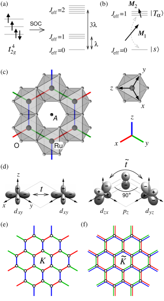
Figure 1: (a) Energy levels of $t_{2g}^{4}$ configuration in $LS$ coupling scheme. Low-energy $J_{\mathrm{eff}}=0$ singlet and $J_{\mathrm{eff}}=1$ triplet form the local basis of our effective model. (b) The magnetic moment consists of dominant van Vleck-type contribution $\boldsymbol{M}_{1}$ residing on the $J_{\mathrm{eff}}=0\leftrightarrow 1$ transition, and a smaller contribution $\boldsymbol{M}_{2}$ carried by $J_{\mathrm{eff}}=1$ triplet. (c) Top view of the honeycomb lattice of edge-shared RuO₆ octahedra in $A_{2}$RuO₃. Cubic axes $x$, $y$, $z$ pointing from Ru towards O ions, as well as the three types (red, green, blue) of nearest-neighbor bonds in the honeycomb lattice are indicated. (d) Hopping within Ru₂O₂ plaquette of a $z$-bond proceeds through direct overlap of $d$ orbitals (left) or indirectly via oxygen ions (right). (e) Kitaev-like pattern of active bond colors for the interaction $K$ in Eq. (10) in the direct-hopping case. On $z$-bonds, the blue-color triplons $T_{z}$ are active, etc. (f) Complementary $xy$-type pattern for the interaction $\tilde{K}$ emerging in the case of indirect hopping; on $z$-bonds, the red ($T_{x}$) and green ($T_{y}$) color triplons are active.

We consider a transition metal ion with four electrons on $t_{2g}$ level, e.g. Ru⁴⁺. Spin-orbit coupling results in a multiplet structure shown in Fig. 1(a). A minimal model for magnetism of such van Vleck-type ions includes the lowest excited $J_{\mathrm{eff}}=1$ states $|T_{\pm 1}\rangle$ and $|T_{0}\rangle$, in addition to the ground state $J_{\mathrm{eff}}=0$ singlet $|s\rangle$. It is convenient to work with three triplon operators $T_{\alpha}$ of Cartesian flavors (“colors”) $\alpha=x,y,z$. Using the above $J_{z}$ eigenstates, they are defined as

$$T_{x}=\tfrac{1}{i\sqrt{2}}(T_{1}-T_{-1}),\;T_{y}=\tfrac{1}{\sqrt{2}}(T_{1}+T_{-1}),\;T_{z}=iT_{0},$$ (1)

and together form a Cartesian vector $\boldsymbol{T}$. A constraint $n_{x}+n_{y}+n_{z}+n_{s}=1$ with $n_{\alpha}=T^{\dagger}_{\alpha}T_{\alpha}$ and $n_{s}=s^{\dagger}s$ is implied. Spin-orbit splitting reads then as a chemical potential for $T_{\alpha}$ bosons: $\lambda\,n_{T}=\lambda\,(n_{x}+n_{y}+n_{z})$.

As illustrated in Fig. 1(b), local magnetic moment is composed of two terms, $\boldsymbol{M}=\boldsymbol{M}_{1}+\boldsymbol{M}_{2}$, where $\boldsymbol{M}_{1}$ originates from dipolar-active transitions between $s$ and $T_{\alpha}$ states [12]:

$$\boldsymbol{M}_{1}=2\sqrt{6}\,\boldsymbol{v}=-\sqrt{6}\,i\,(s^{\dagger}\boldsymbol{T}-\boldsymbol{T}^{\dagger}s),$$ (2)

while $\boldsymbol{M}_{2}$ is derived from triplon-spin $\boldsymbol{J}=-i(\boldsymbol{T}^{\dagger}\times\boldsymbol{T})$ with $g$-factor $1/2$:

$$\boldsymbol{M}_{2}=\tfrac{1}{2}\boldsymbol{J}=-\tfrac{1}{2}\,i\,(\boldsymbol{T}^{\dagger}\times\boldsymbol{T}).$$ (3)

In Eq. (2), $\boldsymbol{v}=-\frac{1}{2}i(s^{\dagger}\boldsymbol{T}-\boldsymbol{T}^{\dagger}s)$ keeps track of the imaginary part of $\boldsymbol{T}$ (real part of $\boldsymbol{T}$ carries a quadrupolar moment).

Triplon interactions are derived from Kugel-Khomskii-type exchange Hamiltonian, projected onto singlet-triplet basis [12; 17]. In honeycomb lattice of the edge-shared RuO₆ octahedra, see Fig. 1(c), there are two types of electron exchange processes, generated by (i) a direct hopping $t$ of $d$-electrons between nearest-neighbor (NN) Ru ions, and (ii) indirect hopping $\tilde{t}$ via oxygen ions, as depicted in Fig. 1(d). Consider, for example, direct $t$-hopping; for a $z$-type bond, it reads as $-t(d_{xy,i}^{\dagger}d_{xy,j}^{\phantom{\dagger}}+\mathrm{H.c.})$. Second order perturbation theory gives the exchange Hamiltonian, written in terms of spin $S=1$ and orbital $L=1$ operators of $d^{4}$ configuration:

$$\mathcal{H}_{ij}^{(z)}=\frac{t^{2}}{U}\,\left[(\boldsymbol{S}_{i}\cdot\boldsymbol{S}_{j}+1)L_{zi}^{2}L_{zj}^{2}\!-\!L_{zi}^{2}\!-\!L_{zj}^{2}\right].$$ (4)

Next, one has to calculate the matrix elements of operators in Eq. (4) between $J_{\mathrm{eff}}=0$ and $J_{\mathrm{eff}}=1$ wavefunctions [12], and represent them in terms $T_{\alpha}$ and $s$. For example, $S^{z}L_{z}^{2}=\sqrt{\frac{8}{3}}\;v_{z}$, while $S^{x/y}L_{z}^{2}=\sqrt{\frac{2}{3}}\;v_{x/y}+\frac{1}{2}J_{x/y}$, with “van-Vleck” moments $\boldsymbol{v}$ and triplon-spin $\boldsymbol{J}$ already defined above. The projected Hamiltonian (4) takes the form of $\mathcal{H}_{ij}^{(z)}=\frac{8}{3}\frac{t^{2}}{U}(h_{2}+h_{3}+h_{4})^{(z)}_{ij}$. It contains two-, three-, and four-triplon operator terms:

$$h_{2}^{(z)} =v_{zi}v_{zj}+\frac{1}{4}(v_{xi}v_{xj}+v_{yi}v_{yj}),$$ (5)

$$h_{3}^{(z)} =\frac{1}{8}\sqrt{\frac{3}{2}}(v_{xi}J_{xj}+v_{yi}J_{yj})+(i\leftrightarrow j),$$ (6)

$$h_{4}^{(z)} =\frac{3}{32}(J_{xi}J_{xj}+J_{yi}J_{yj})+\frac{1}{32}\,Q_{3i}Q_{3j},$$ (7)

where $Q_{3}=(n_{x}+n_{y}-2n_{z})/\sqrt{3}$ is a quadrupole operator of $E_{g}$ symmetry. Interactions $\mathcal{H}_{ij}^{(x)}$ and $\mathcal{H}_{ij}^{(y)}$ for $x$- and $y$-type bonds follow from symmetry. The largest term in the above Hamiltonian is represented by $v_{zi}v_{zj}$ coupling in $h_{2}$; physically, this is Ising-type coupling between van-Vleck moments.

Indirect hopping via ligands $-\tilde{t}(d_{yz,i}^{\dagger}d_{zx,j}^{\phantom{\dagger}}+\mathrm{H.c.})$ generates triplon Hamiltonian of the same form, $\mathcal{\tilde{H}}_{ij}^{(z)}=3\frac{\tilde{t}^{2}}{U}(\tilde{h}_{2}+\tilde{h}_{3}+\tilde{h}_{4})^{(z)}_{ij}$. In contrast to the above case, however, a dominant term here is represented by $xy$-type coupling $(v_{xi}v_{xj}+v_{yi}v_{yj})$ in $\tilde{h}_{2}$ (explicit forms of the other terms can be found in Ref. [12]).

The full models $\mathcal{H}$ and $\mathcal{\tilde{H}}$ are clearly rich but complicated; considering their dominant terms represented by Ising- and $xy$-type couplings between $v$-moments should provide some useful insights. Even though these couplings look as simple quadratic forms, the hard-core nature of triplons and their bond-directional anisotropy lead to nontrivial consequences [12; 17].

We introduce the bond operator $\mathcal{O}_{ij}^{\alpha}=4v_{\alpha i}v_{\alpha j}$, which in terms of singlet $s$ and triplon $T_{\alpha}$ operators reads as:

$$\mathcal{O}_{ij}^{\alpha}=T^{\dagger}_{\alpha i}s^{\phantom{\dagger}}_{i}s^{\dagger}_{j}T^{\phantom{\dagger}}_{\alpha j}-T^{\dagger}_{\alpha i}s^{\phantom{\dagger}}_{i}T^{\dagger}_{\alpha j}s^{\phantom{\dagger}}_{j}+\mathrm{H.c.}$$ (8)

We recall that $s$ and $T_{\alpha}$ are subject to local constraint $n_{s}+n_{T}=1$. Alternatively,

$$\mathcal{O}_{ij}^{\alpha}=\mathcal{T}^{\dagger}_{\alpha i}\mathcal{T}^{\phantom{\dagger}}_{\alpha j}-\mathcal{T}^{\dagger}_{\alpha i}\mathcal{T}^{\dagger}_{\alpha j}+\mathrm{H.c.},$$ (9)

where $\mathcal{T}^{\dagger}=T^{\dagger}s$ is a hard-core boson with $n_{\mathcal{T}}\leq 1$. In terms of $\mathcal{O}_{ij}^{\alpha}$, a minimal singlet-triplet model Hamiltonian can concisely be written as

$$\mathcal{H}=\sum_{i}E_{T}\,n_{T_{i}}+\sum_{{\langle ij\rangle}_{\alpha}}[K\mathcal{O}_{ij}^{\alpha}+\tilde{K}(\mathcal{O}_{ij}^{\bar{\alpha}}+\mathcal{O}_{ij}^{\bar{\bar{\alpha}}})].$$ (10)

Here, the color $\alpha\in\{x,y,z\}$ is given by the direction of the bond $\langle ij\rangle$, and $\bar{\alpha}$, $\bar{\bar{\alpha}}$ are the two complementary colors; e.g., for $z$-type bond $\langle ij\rangle_{z}$ one has $\alpha=z$, while $\bar{\alpha}=x$ and $\bar{\bar{\alpha}}=y$. As derived, the model parameters are $E_{T}=\lambda$, $K=\frac{2}{3}t^{2}/U$, $\tilde{K}=\frac{1}{4}K+\frac{3}{4}\tilde{t}^{\>2}/U$.

The $K$ ($\tilde{K}$) term in Eq. (10) features Kitaev-like ($xy$-type) symmetry, with one (two) active components of $\boldsymbol{T}$-vector on a given bond. The resulting color-and-bond selective interaction patterns $K$ and $\tilde{K}$ are shown in Fig. 1(e) and Fig. 1(f), correspondingly. At $K=\tilde{K}$, the model is equivalent to a conventional O(3) singlet-triplet models [22] that appear, e.g., in low-energy description of a bilayer Heisenberg system. In this isotropic limit, the model is free of frustration and would undergo a magnetic transition at large enough coupling strength $K\sim E_{T}$. In this paper, the Kitaev-like model with $K$-term, where triplon dynamics is most frustrated, is of primary interest. In particular, we are interested in the nature of magnetically disordered ground state at strong coupling limit of $K\gg E_{T}$. In real materials, an admixture of the complementary interaction $\tilde{K}$ is expected, and we will consider its impact on the phase behavior of the model.

III Symmetry properties and links to Kitaev honeycomb model

The color–bond correspondence of the above model in the $K\neq 0$, $\tilde{K}=0$ case is strongly reminiscent of the Kitaev honeycomb model. In this section, we focus exclusively on this limit, draw the corresponding analogies, and find an exact link between our model and a particular variant of bilayer Kitaev model.

III.1 Extensive number of conserved quantities

In the Kitaev-like limit of the model in Eq. (10), i.e. $\tilde{K}=0$, the number of $T_{\alpha}$ stays either even ($0$ and $2$) or odd ($1$) on a bond of direction $\alpha$. The parity of this number is thus a conserved $Z_{2}$ quantity that can be formally written as

$$P_{ij}=(1-2n_{\alpha i})(1-2n_{\alpha j})$$ (11)

with $n_{\alpha i}$ counting $T_{\alpha}$-triplon number on site $i$. Being associated with the individual bonds, the parities form an extensive set of conserved $Z_{2}$ quantities that decompose the Hilbert space into subspaces with fixed bond-parity configurations. The total Hilbert space dimension equals $4^{N}$ for a system with $N$ sites. With one $Z_{2}$ conserved quantity per bond (amounting to $\frac{3}{2}$ per site), the average subspace dimension is reduced to $4^{N}/2^{\frac{3N}{2}}=(\sqrt{2})^{N}$. This is actually the same scaling as in the case of the Kitaev honeycomb model [7], where the conserved $Z_{2}$ quantities are associated with hexagonal plaquettes (giving $\frac{1}{2}$ of $Z_{2}$ quantity per site) and the average subspace dimension thus becomes $2^{N}/2^{\frac{N}{2}}=(\sqrt{2})^{N}$. In accord with intuitive expectation, our numerical calculations found the ground state to have all-even bond-parity configuration.

III.2 Mapping to hardcore bosons on a dual lattice

When working in the subspaces with fixed bond parities, most of the $4^{N}$ configurations of triplons on the honeycomb lattice of size $N$ are irrelevant. To remove this redundancy in the description, here we develop an auxiliary particle representation by mapping to a system of spinless hardcore bosons on dual (kagomé) lattice.

For simplicity, we limit ourselves to the case of all-even bond parities, similar one-to-one mappings can be found also in the other cases. The mapping is illustrated in Fig. 2(a). A given bond of the honeycomb lattice can either be occupied by a pair of triplons of the proper color or be empty. These two states are represented by the presence/absence of a hardcore boson $b$ on the corresponding dual lattice site. Starting from a $b$-configuration, the state of a given honeycomb site can be uniquely reconstructed by checking the surrounding kagomé sites for $b$ bosons. Either (i) one of them is found, selecting one of the $T_{\alpha}$ states with $\alpha$ depending on the bond occupied by the $b$ boson, or (ii) none is present, corresponding to the “empty” states $s$. The constraint for the $b$ bosons is now evident – a nearest-neighbor pair of $b$ at the dual lattice is forbidden.

Altogether, we can formulate the Hamiltonian for the $b$ bosons on the dual lattice as

$$\mathcal{H}_{\mathrm{dual}}=\sum_{i}[2E_{T}n_{b}-K(b+b^{\dagger})]_{i}+U\sum_{\langle ij\rangle}n_{bi}n_{bj},$$ (12)

where $i$ runs through the sites of the kagomé lattice, and the repulsive interaction with $U\rightarrow\infty$ enforces the constraint of “no nearest-neighbor occupation” for $b$ bosons. Without this constraint, the sum of local Hamiltonians in (12) would be easy to diagonalize leading to bond eigenstates that involve $|ss\rangle$ and $|T_{\alpha}T_{\alpha}\rangle$ pairs. In the form of Eq. (12), the peculiarity of the model is fully exposed – the $K$ interaction forms bond dimers that communicate via constraint only. Adding intersite hopping terms $b^{\dagger}_{i}b_{j}$ in the model would generate boson dispersion and phase relations between them on different sites, leading to a superfluid condensate; however, we have so far no clear microscopic mechanism that would result in such a triplon-pair hopping process.

Finally, let us recall that the above $\mathcal{H}_{\mathrm{dual}}$ is valid for the all-even sector only; the formulation of the constraint in the other cases is more complicated.

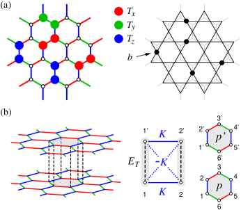
Figure 2: (a) Sample triplon configuration on the honeycomb lattice (left) and the corresponding configuration of spinless hardcore bosons $b$ (black dots) on a dual kagomé lattice (right). In the case of all-even bond parities depicted here, the presence of a $T$-dimer with a proper color (i.e. same as that of the bond) is represented by $b$ boson on the dual lattice. No nearest-neighbor pairs of $b$ on a kagomé lattice is allowed. (b) Equivalent spin-$\frac{1}{2}$ bilayer model realizing the singlet-triplet basis on interlayer vertical bonds that are subject to Heisenberg interaction $J=E_{T}$. In the model, Kitaev interaction $K$ active on intralayer bonds (such as $1-2$ and $1^{\prime}-2^{\prime}$) is complemented by a Kitaev interaction $-K$ of opposite sign, acting on interlayer cross links (such as $1-2^{\prime}$ and $1^{\prime}-2$). Vertically adjacent hexagonal plaquettes $p$, $p^{\prime}$ are used to construct the conserved quantities.

III.3 Local nature of the spin correlations

Similarly to the Kitaev model, the presence of the local conserved quantities has consequences for the spin correlations, both of van Vleck moments of Eq. (2) as well as triplon spins entering Eq. (3). Let us consider static correlations of the type $\langle M_{\alpha}M_{\alpha}\rangle=Z^{-1}\sum_{n}\langle n|M_{\alpha}M_{\alpha}|n\rangle\,\mathrm{e}^{-\beta E_{n}}$ or the corresponding dynamic correlations. The eigenstates $|n\rangle$ of Eq. (10) with $\tilde{K}=0$ have fixed bond-parity configurations. When acting by the $\alpha$-component of the van Vleck moment operator $M_{1\alpha}\propto(s^{\dagger}T^{\phantom{\dagger}}_{\alpha}-T^{\dagger}_{\alpha}s)$ on a given site, the bond parity of the attached $\alpha$-bond is switched. Bond parities are conserved by the Hamiltonian, the introduced parity defect is thus immobile, and to get back to original parity configuration, one has to act with $M_{1\alpha}$ either at the same site or on the second site of the affected $\alpha$-bond. Therefore, $\langle M_{\alpha}M_{\alpha}\rangle$ correlator is strictly zero beyond a nearest-neighbor distance. Similarly, the triplon spin operator $-i(\boldsymbol{T}^{\dagger}\times\boldsymbol{T})$ flips parities of two attached bonds, the original bond-parity configuration therefore has to be restored by acting at the same site. As a result, the Kitaev-like limit of the model is characterized by nearest-neighbor only correlations of the magnetic moments (stemming from the van Vleck component matching the bond color), and a localized nature of the dynamic spin response. This mechanism is completely analogous to the Kitaev model, where a spin flip introduces two localized fluxes [7].

III.4 Links to the Kitaev honeycomb model

In the previous Secs. III.1 and III.3 we have noticed several striking similarities between the bosonic $K$-model and Kitaev’s model for spins-$\frac{1}{2}$ residing on the honeycomb lattice. A deeper connection of the two models can be thus anticipated, motivating the search for a spin-$\frac{1}{2}$ equivalent of our model that could reveal such a link. A natural search direction is the class of bilayer spin-$\frac{1}{2}$ systems with Heisenberg interlayer interaction forming a local singlet-triplet basis on the interlayer rungs.

Indeed, the Hamiltonian in Eq. (10) can be exactly mapped onto spin-$\frac{1}{2}$ bilayer honeycomb system with the interactions $K$ and $\tilde{K}$ transforming into nearest-neighbor intralayer links and second nearest-neighbor interlayer links as depicted in Fig. 2(b). For $\tilde{K}=0$, the Hamiltonian involving the nearest-neighbor bond $1$-$2$ and the adjacent one $1^{\prime}$-$2^{\prime}$ in the other layer reads as

$$\mathcal{H}_{121^{\prime}2^{\prime}}=E_{T}(\boldsymbol{S}_{1}\boldsymbol{S}_{1^{\prime}}+\boldsymbol{S}_{2}\boldsymbol{S}_{2^{\prime}})\\ +K(S^{\alpha}_{1}S^{\alpha}_{2}+S^{\alpha}_{1^{\prime}}S^{\alpha}_{2^{\prime}})-K(S^{\alpha}_{1}S^{\alpha}_{2^{\prime}}+S^{\alpha}_{1^{\prime}}S^{\alpha}_{2}).$$ (13)

The first two terms form nothing but a pair of Kitaev models linked by vertical Heisenberg bonds. This so-called bilayer Kitaev model was recently studied in Refs. [18; 20; 19]. The last term in Eq. (13) provides additional Kitaev-like cross-links of the sign opposite to the intra-layer Kitaev interaction and, as we find later, drastically changes the behavior of the system from that of standard bilayer Kitaev model.

With the above mapping, we are ready to consider the relations between various local conserved quantities. The single layer Kitaev model conserves the product of spin operators at a hexagonal plaquette [see Fig. 2(b)]

$$W_{p}=2^{6}S^{x}_{1}S^{y}_{2}S^{z}_{3}S^{x}_{4}S^{y}_{5}S^{z}_{6}.$$ (14)

In a bilayer Kitaev model, one has to construct products $W_{p}W_{p^{\prime}}$ of Kitaev’s $W_{p}$ for vertically adjacent plaquettes [18]. These conserved $Z_{2}$ quantities bring about certain features of Kitaev physics to the bilayer Kitaev model. In the case of our model (13), the extra Kitaev-like cross-links are present. However, the products $W_{p}W_{p^{\prime}}$ are still conserved, as can be verified by a direct calculation. Surprisingly, this does not make them yet another set of conserved quantities. In fact, it turns out that $W_{p}W_{p^{\prime}}$ are merely products of our bond parities $P_{ij}$

$$W_{p}W_{p^{\prime}}=P_{12}P_{23}P_{34}P_{45}P_{56}P_{61}$$ (15)

in the original formulation, and appear as a simple consequence of the bond-parity conservation in the model. The above connection also translates the all-even parity configuration of the ground state into the absence of fluxes in the ground state, i.e. $W_{p}W_{p^{\prime}}=+1$ for all plaquettes. The local symmetries of our model are thus more powerful than in the Kitaev model or its simple bilayer extension. Intuitively it may be expected that this denser covering by local conserved quantities will lead to less entangled (more factorized) ground states, as we indeed find below.

As a side remark, we note that while the Hamiltonian (10) contains a balanced combination of hopping and pair terms, differing only by the sign [see Eq. (9)], it is possible to generalize the above mapping to the case $A\,T^{\dagger}_{\alpha}T_{\alpha}-B\,T^{\dagger}_{\alpha}T^{\dagger}_{\alpha}+\mathrm{H.c.}$ with $A\neq B$. The resulting spin-$\frac{1}{2}$ interactions consist of $\mathcal{H}_{121^{\prime}2^{\prime}}$ of Eq. (13) with $K=\tfrac{1}{2}(A+B)$ and an additional four-spin interaction

$$\Delta\mathcal{H}_{121^{\prime}2^{\prime}}=2(A-B)(\boldsymbol{S}_{1}\times\boldsymbol{S}_{1^{\prime}})^{\alpha}(\boldsymbol{S}_{2}\times\boldsymbol{S}_{2^{\prime}})^{\alpha}.$$ (16)

By introducing symmetric off-diagonal exchange $\Gamma_{ij}=S_{i}^{x}S_{j}^{y}+S_{i}^{y}S_{j}^{x}$ (for a $z$ bond, $x$ and $y$-bond expressions are obtained by cyclic permutation), it can be brought to a form $2(B-A)(\Gamma_{12}\Gamma_{1^{\prime}2^{\prime}}-\Gamma_{12^{\prime}}\Gamma_{1^{\prime}2})$ resembling somewhat the structure in Eq. (13). All the arguments concerning conserved quantities remain valid also in the $A\neq B$ case, because the original interactions in expressed using the $T$ particles manifestly conserve bond parities. For example, despite the complicated structure of Eq. (16), it commutes with the plaquette products $W_{p}W_{p^{\prime}}$ keeping them still conserved.

IV Kitaev-like singlet-triplet zigzag chain

Before studying the full model on the honeycomb lattice, we first focus on its one-dimensional analog. The 1D system is more accessible to numerics and enables easier insights. As an example of such an approach in the context of the Kitaev-Heisenberg model, Ref. [23] studies the corresponding 1D chains and subsequently makes an interpretation of the 2D honeycomb model behavior in terms of coupled 1D chains.

To form a 1D model analogous to the honeycomb one, we remove $T_{z}$ triplon and keep only one zigzag chain of the honeycomb lattice, consisting of $x$ and $y$ bonds. In the Kitaev-like limit $\tilde{K}=0$, these two changes are equivalent as only $T_{z}$ is active on the $z$ bonds. Going away from the Kitaev-like limit, as an alternative to the complementary $\tilde{K}$ interaction, it is more transparent here to add bond-independent $J_{\mathrm{XY}}$ interaction. Instead of the model in Eq. (10) we therefore deal with

$$\mathcal{H}=\sum_{i}E_{T}\,n_{T_{i}}+\sum_{{\langle ij\rangle}_{\alpha}}[K\mathcal{O}_{ij}^{\alpha}+J_{\mathrm{XY}}(\mathcal{O}_{ij}^{x}+\mathcal{O}_{ij}^{y})]$$ (17)

formulated for a zigzag chain of alternating $x$ and $y$ bonds with the bond direction determining again the color $\alpha$. Note that for $J_{\mathrm{XY}}\neq 0$, a slight change to the original parametrization occurs: $K=(K-\tilde{K})_{\mathrm{orig}}$, $J_{\mathrm{XY}}=\tilde{K}_{\mathrm{orig}}$.

Having now only three levels $s$, $T_{x}$, $T_{y}$ in the 1D model, it is possible to convert it to a spin-$1$ chain using the transformation

$$S^{x} =-i(s^{\dagger}T^{\phantom{\dagger}}_{x}-T^{\dagger}_{x}s),$$ (18)

$$S^{y} =-i(s^{\dagger}T^{\phantom{\dagger}}_{y}-T^{\dagger}_{y}s),$$ (19)

$$S^{z} =-i(T^{\dagger}_{x}T^{\phantom{\dagger}}_{y}-T^{\dagger}_{y}T^{\phantom{\dagger}}_{x}),$$ (20)

where the first two components of the effective spin-$1$ correspond to van Vleck moments $\boldsymbol{v}$ while the last one is linked to the triplon spin $\boldsymbol{J}$ [see Eqs. (2) and (3)]. The resulting equivalent spin-$1$ model is a Kitaev-XY spin-$1$ chain with single-ion anisotropy $E_{T}$:

$$\mathcal{H}=\sum_{i}E_{T}(S_{i}^{z})^{2}+\sum_{{\langle ij\rangle}_{\alpha}}[KS_{i}^{\alpha}S_{j}^{\alpha}+J_{\mathrm{XY}}(S_{i}^{x}S_{j}^{x}+S_{i}^{y}S_{j}^{y})].$$ (21)

The phase diagram of this model for the $K=0$ case (no bond-alternation) was thoroughly explored in the context of spin-$1$ XXZ chain with single-ion anisotropy (see, e.g., Refs. [24; 25; 26; 27]). Later in Sec. IV.2, we will use these corresponding studies as a reference.

IV.1 Chain with pure Kitaev-like interaction

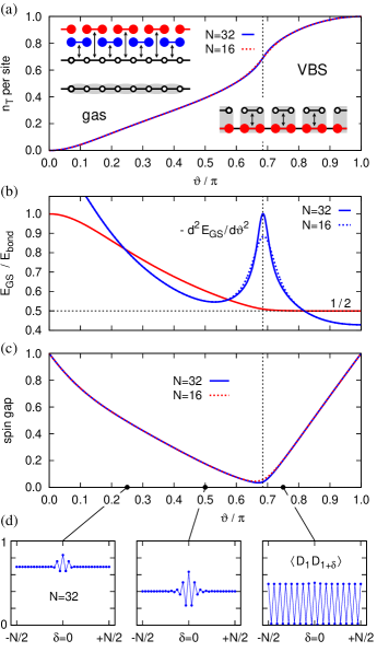
Figure 3: (a) Occupation of the triplon states $T_{x,y}$ within the chain model parametrized as $E_{T}=\cos\vartheta$, $K=\sin\vartheta$ obtained by exact diagonalization. Results for the chains of the length $N=16$ and $N=32$ are nearly identical. The insets show a cartoon picture of the groundstate: At positive $E_{T}\gg K$, each bond can be predominantly in the bonding state as it is mostly composed of $s$. At negative $E_{T}$ with $|E_{T}|\gg K$, the bonding states are incompatible and are realized only on every second bond creating thus a valence bond solid. (b) Ground-state energy per bond $E_{\mathrm{GS}}$ measured by bonding state energy $E_{\mathrm{bond}}$ (red) and the second derivative of $E_{\mathrm{GS}}$ with respect to $\vartheta$ revealing the quantum critical point (blue). (c) Spin gap obtained as the difference of ground-state energies within all-even sector and the sector with a single odd-parity bond. (d) Examples of bond-dimer correlations $\langle D_{1}D_{1+\delta}\rangle$ with the dimer operator defined as a projector to the bonding state of Eq. (22): $D=|B\rangle\langle B|$. The value of the correlator at $\delta=0$ gives the probability of the bonding state $P_{B}$, at large distances it approaches $P_{B}^{2}$ in the gas phase. Oscillations near $\delta=0$ growing with $\vartheta$ are due to the increasing incompatibility of bonding states at adjacent bonds. The correlation length diverges approaching the QCP and long-range correlations are seen in the VBS phase.

As the first step, we consider the Kitaev-like limit of the model (17), i.e. neglecting $J_{XY}$ term. In general, the behavior of all our models is determined by a competition of the triplon energy cost $E_{T}$ with the energy gain due to the interactions. One can thus expect a quantum critical point (QCP) separating a triplon gas phase with small triplon densities (dominant $E_{T}$ regime) from a phase characterized by strongly interacting triplons at larger densities (dominant $K$ regime).

Such a competition is captured by Fig. 3 presenting an evolution for varying $K$ to $E_{T}$ ratio. For a better understanding and to actually reach the QCP in this case, we have extended the parameter range to the (non-realistic in the present physical context but interesting theoretically) regime of $E_{T}<0$ with reversed $s$ and $T$ levels. The data obtained by exact diagonalization (ED) are shown for two chain lengths to assess the finite-size effects that are quite small here. As seen in Fig. 3(a), for an increasing interaction strength $K$, the triplon density $n_{T}$ gradually increases with just a single hint of a change of the regime located already at negative $E_{T}$. This QCP is clearly revealed by the second derivative of the ground-state energy $E_{\mathrm{GS}}$ with respect to model parameters as presented in Fig. 3(b).

To understand the energetics of the evolution together with the nature of the two phases, it is convenient to measure the chain $E_{\mathrm{GS}}$ per bond by a ground-state energy of an isolated bond, as it is done in Fig. 3(b). The ground state of a single bond – the bonding state – mixes a pair of proper-color triplons and a pair of $s$ in the wavefunction

$$|B\rangle=\cos\phi\,|ss\rangle+\sin\phi\,|T_{\alpha}T_{\alpha}\rangle$$ (22)

with $\phi$ given by $\tan 2\phi=K/E_{T}$, and has the energy $E_{\mathrm{bond}}=E_{T}-\sqrt{E_{T}^{2}+K^{2}}$. This approximately evaluates to $-K^{2}/2E_{T}$ for small $K$, capturing the perturbative incorporation of a triplon pair (energy $2E_{T}$) by a process with an amplitude $K$. The orthogonal combination to $|B\rangle$ is the antibonding state $|A\rangle=\cos\phi\,|T_{\alpha}T_{\alpha}\rangle-\sin\phi\,|ss\rangle$ whose energy starts at $2E_{T}$ in $K\rightarrow 0$ limit. Similarly to $n_{T}$, the ground-state energy measured by $E_{\mathrm{bond}}$ shows a gradual evolution with the model parameters for most of the parameter range apart from a change at QCP [see Fig. 3(b)]. In the $E_{T}\gg K$ regime, $E_{\mathrm{GS}}$ reveals the dominance of the bonding states that seem to fill up the system. This is possible since the bonding states are composed mostly of $s$ states that can be shared by the neighboring bonds. For increasing $K$ and thus an increasing admixture of $T$ pairs with bond-dependent color, the bonding states at neighboring bonds have less overlap and the energy gain from $K$ is reduced compared to that of isolated bonds. At the QCP, $E_{\mathrm{GS}}/E_{\mathrm{bond}}$ approaches $\frac{1}{2}$ and stays flat indicating a valence bond solid (VBS) phase with a rigid structure where every second bond hosts a bonding state. A more detailed inspection shows that in the VBS phase, $E_{\mathrm{GS}}/E_{\mathrm{bond}}$ positively deviates from $\frac{1}{2}$ with the difference scaling as $K^{6}$. This energy gain can be understood within second order perturbation theory as an effect of virtual processes where two neighboring $T$ pairs disappear to make space for an emerging middle $T$ pair (total amplitude is $K^{3}$) being an intermediate state.

Interestingly, the smooth evolution observed in Fig. 3 suggests a picture of the dilute triplon gas at $E_{T}\gg K$ being continuously connected with the dense triplon state close to the QCP. It is further supported by a gradual reduction of the spin gap closing at QCP Fig. 3(c) and an exponential decay of dimer correlations [Fig. 3(d)] with the decay length diverging at QCP when the VBS is formed.

In the Kitaev model, the spin gap separates the flux-free ground state from the topological sector with two fluxes. Within this gap, excitations from the flux-free sector carried by itinerant Majorana fermions can be found. In our model, the spin gap shown in Fig. 3(c) separates the ground state with all-even bond configuration and the sector with one odd bond that is being flipped by the van Vleck moment operator. However, in contrast to the Kitaev model, here the excitation to one-odd sector is lower than excitations within all-even sector all the way up to QCP. In other words, no modes (e.g. Majorana bands) are present within the spin-gap. At the QCP, the lowest excitations merge, including also partly the lowest excitations to the other sectors with more odd bonds. The special role of the QCP will be further demonstrated in the next section – an antiferromagnetic condensate will be found to emanate from it and an intuitive picture of the critical excitations near QCP will be inferred.

IV.2 Extension towards XY-chain

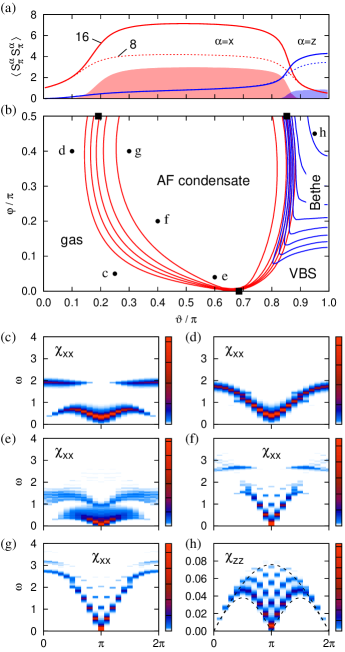
Figure 4: (a) Correlations $\langle S^{\alpha}_{q}S^{\alpha}_{-q}\rangle$ with $q=\pi$ for the chain model with $K=0$ parametrized as $E_{T}=\cos\vartheta$, $J_{\mathrm{XY}}=\sin\vartheta$. Data for chains of the length $N=16$ and $N=8$ are shown. Their difference (shaded areas) represents the part of the correlations scaling with the system size and could be used to estimate the extent of the corresponding phases. (b) Approximate phase diagram of $E_{T}-K-J_{\mathrm{XY}}$ model parametrized as $E_{T}=\cos\vartheta$, $K=\sin\vartheta\cos\varphi$, $J_{\mathrm{XY}}=\sin\vartheta\sin\varphi$. The contours capture the difference of the correlations $\langle S^{\alpha}_{\pi}S^{\alpha}_{\pi}\rangle$ between $N=16$ and $N=8$ chains. Red and blue lines are based on $S^{x}$ and $S^{z}$ correlations, respectively. Black squares are reference points from Langari et al. [28] ($\varphi=\pi/2$ line) and from Fig. 3 ($\varphi=0$ line). The top line with $\varphi=\pi/2$ matches panel (a). (c)–(h) Imaginary part of $S^{x}$ or $S^{z}$ susceptibilities calculated for a chain with $N=20$ sites at the selected parameter points marked in panel (b). Panel (h) shows also the boundaries (dashed lines) of the excitation continuum for the effective spin-$\frac{1}{2}$ Heisenberg chain.

Having explored the Kitaev-like limit of the model on the chain, we now consider its extension by $J_{XY}$-interaction introduced in Eqs. (17) and (21). As our main interest is the qualitative illustration of the concepts that appear in the honeycomb case as well, we do not focus on the specifics that are related to one-dimensionality but rather on the generic features that will be inherited by the 2D lattice case.

Let us start the discussion with the pure XY-limit where our model can be related to spin-$1$ XXZ chain with single-ion anisotropy for which extensive studies are available [24; 25; 26; 27; 28], mainly in the connection with the Haldane gap problem. Its phase diagram is quite complex containing a number of phases depending on the $J_{\mathrm{Z}}/J_{\mathrm{XY}}$ ratio and single-ion anisotropy $D$ [corresponding to our $E_{T}$ in Eq. (21)]: large-$D$ phase, Haldane phase, two XY phases, the ferromagnetic phase, and the Néel phase [27]. For the relevant $J_{\mathrm{Z}}=0$ case that matches to our model, it shows two quantum critical points. The first one at $E_{T}\approx 0.34J_{\mathrm{XY}}$ corresponds to the transition between the large-$D$ phase and the Haldane phase and its precise determination requires the detection of topological features of the Haldane phase such as the edge spin-$\frac{1}{2}$ pair [27]. The second transition to the Néel phase occurs at $E_{T}\approx-2J_{\mathrm{XY}}$ and in contrast to the first one is easy to capture precisely [28].

The XY-limit of our model is numerically studied in Fig. 4(a) by means of spin correlations obtained by ED. Since the local conserved quantities are lost when introducing the $J_{\mathrm{XY}}$ interaction, we are now limited to a shorter chain length (at most $N=20$ sites) compared to the previous paragraph. We employ both van Vleck moments [$S^{x}$ and $S^{y}$ components of the effective spin-$1$ defined by Eqs. (18), (19)] and triplon spin [$S^{z}$ component defined in Eq. (20)]. The static correlators $\langle S^{\alpha}_{q}S^{\alpha}_{-q}\rangle$ of their Fourier components $S^{\alpha}_{q}=\sum_{l=1}^{N}S^{\alpha}_{l}\exp(-iql)/\sqrt{N}$ at the characteristic momentum $q=\pi$ are plotted for two different lengths of the chain and subtracted. The difference uncovers a correlation contribution scaling with the system size (on top of a size-independent contribution) that we regard as a signature of a particular phase. Though oversimplified compared to a full finite-size scaling analysis, this approach will later provide a rough sketch of the phase diagram of the model in its entire parameter space.

Figure 4(a) shows three regimes of the correlations for the XY limit. The first one for $E_{T}\gg J_{\mathrm{XY}}$ corresponds to the triplon gas with the correlations generated exclusively by triplon excitations. It is quickly replaced at about $E_{T}\approx 1.5J_{\mathrm{XY}}$ with a triplon condensate characterized by antiferromagnetic (AF) correlations of van Vleck moments $M_{1\alpha}\propto(s^{\dagger}T^{\phantom{\dagger}}_{\alpha}-T^{\dagger}_{\alpha}s)$. An intuitive picture of the condensate can be based on a trial ground-state wavefunction that explicitly mixes the condensed $T$ states into a “pool” of $s$ states

$$|\Psi\rangle=\prod_{l=1}^{N}\left(\sqrt{1-\rho}\,|s\rangle+\sqrt{\rho}\,\;i\,\mathrm{e}^{i\pi l}\;|T\rangle\right)_{l},$$ (23)

creating thus van Vleck moments. Here $|T\rangle$ stands for any normalized combination of $|T_{x}\rangle$ and $|T_{y}\rangle$ and $\rho$ is the condensate density, $0\leq\rho\leq 1$. At each site $l$ the hardcore condition $n_{T}\leq 1$ is obeyed. While the wavefunction (23) is more appropriate for the 2D case with static long-range AF order, it still captures the transition between the regime of a triplon gas ($\rho=0$) and the condensate with pronounced AF correlations ($\rho>0$) and gives a very crude estimate $E_{T}=4J_{\mathrm{XY}}$ of the transition point. This is based on minimizing the energy per site $E_{T}\rho-4J_{\mathrm{XY}}\rho(1-\rho)$ with respect to the variational parameter $\rho$. Later in Sec. V.2, we will develop a quantitative mean-field treatment of the honeycomb model based on the same type of condensation.

The second quantum phase transition (QPT) appearing at $E_{T}\approx-2J_{\mathrm{XY}}$ is to a phase associated with the limit of large negative $E_{T}$. At this transition, the energy gain from negative $E_{T}$ overcomes the energy gain from correlated van Vleck moments and the system collapses to a state full of $T_{x}$ and $T_{y}$ triplons leaving the triplon color as the only active degree of freedom. The costly $s$ state can be integrated out leading to an effective interaction among pseudospins-$\frac{1}{2}$ describing the $T_{x}$, $T_{y}$ doublets. In the isotropic XY case under consideration, the resulting effective model valid for $J_{\mathrm{XY}}\ll-E_{T}$ is simply a spin-$\frac{1}{2}$ Heisenberg chain with the exchange parameter $J_{\mathrm{eff}}=J_{\mathrm{XY}}^{2}/|E_{T}|$. It can be obtained by removing $s$ via second order perturbation theory and introducing the sublattice dependent mapping

$$|T_{x}\rangle \rightarrow|\!\uparrow\rangle, |T_{y}\rangle \rightarrow|\!\downarrow\rangle \text{(even sites)},$$ (24)

$$|T_{x}\rangle \rightarrow|\!\downarrow\rangle, |T_{x}\rangle \rightarrow-|\!\uparrow\rangle \text{(odd sites)}.$$ (25)

Because of the connection to the exactly solvable spin-$\frac{1}{2}$ Heisenberg chain, hereafter we call the corresponding phase the Bethe phase (Néel phase in the context of spin-$1$ XXZ chains).

It has to be noted that while our second QPT for negative $E_{T}$ well corresponds to the reference data by Chen et al. [27], the first change of the regime occurs for much smaller $J_{\mathrm{XY}}$ in our data than in Ref. [27]. On the other hand, we obtain a good agreement with the quantum renormalization group (QRG) and ED study [28] of the ground-state fidelity. This may be interpreted within the triplon condensation picture as follows. The true Haldane phase appears around $E_{T}\approx 0.34J_{\mathrm{XY}}$ but this QPT is preceded much earlier by our “transition” associated with the onset of van Vleck correlations and corresponding to the emergence of a triplon (quasi-)condensate. Such a change in the ground-state structure is also reflected in the ground-state fidelity inspected in Ref. [28]. While probably not a real QPT, it is a crossover determined by the energy balance of the triplon cost and the energy gain due to a formation of correlated van Vleck moments. In non-frustrated situations, this energy balance shall lead to a crossover/transition at similar $J/E_{T}$ ratios, depending mainly on the connectivity of the particular lattice. Therefore, the apparent discrepancy is not essential because in the 2D honeycomb case, the emergence of the condensate will correspond to establishing a real long-range AF order of van Vleck moments.

After discussing both the Kitaev-like limit explored in Sec. IV.1 and the XY-limit in the above, we now extend the correlation-based approach to the full $E_{T}-K-J_{\mathrm{XY}}$ model to obtain a sketch of the phase diagram presented in Fig. 4(b).

The topology of the phase diagram follows from the features already met above when inspecting the limiting cases. Most of the phase diagram, in particular all of its physically sensible part ($E_{T}>0$), is taken up by the competition of the triplon gas and the triplon condensate with AF correlations of van Vleck moments – components $S^{x}$, $S^{y}$ of the effective spin-$1$. The crossover is more and more delayed when going from the XY-limit ($\varphi/\pi=0.5$) to the Kitaev-like one ($\varphi=0$). This is easily understood by an increasing frustration in this direction and thus a smaller gain from creating correlated van Vleck moments. A larger interaction strength is thus needed to overcome the $E_{T}$ cost. The remaining phases are restricted to the area of large negative $E_{T}$. Depending on the balance between $K$ and $J_{\mathrm{XY}}$, the system selects either the VBS phase with every second bond essentially inactivated, or the Bethe phase linked to the hidden effective spin-$\frac{1}{2}$ model – a Heisenberg chain – and revealed by AF correlations of $S^{z}$ components of the effective spin-$1$.

To complement the phase diagram, Figs. 4(c)–(h) present dynamical correlations $\chi_{\alpha\alpha}(q,\omega)=\langle S^{\alpha}_{q}S^{\alpha}_{-q}\rangle_{\omega}$, i.e. spin susceptibility associated with the effective spin-$1$, calculated for several points in the phase diagram. The gapped van Vleck susceptibility $\chi_{xx}=\chi_{yy}$ in Fig. 4(c),(d) for the triplon gas phase shows the difference between the local-like response consisting of two flat parts in the Kitaev-like limit [Fig. 4(c)] and (almost) continuous dispersion at large $J_{\mathrm{XY}}$ [Fig. 4(d)]. Similarly, Figs. 4(e)-(g) capture the evolution from the Kitaev-like to the XY-limit response of the AF condensate. Here the low-energy part is dominated by an intense linear mode centered at the AF wavevector $q=\pi$. Extrapolation of data up to $N=20$ suggests gapless response inside the AF condensate region, within the precision limited by finite-size effects that are pronounced mainly in the transition region. Finally, inspecting the susceptibility $\chi_{zz}$ for a point deep inside the Bethe phase, we notice that the dynamical response clearly reveals the hidden spin-$\frac{1}{2}$ Heisenberg chain. For example, its excitation continuum perfectly matches the expected analytical boundaries obtained using $J_{\mathrm{eff}}=J_{\mathrm{XY}}^{2}/|E_{T}|$, see the dashed lines in Fig. 4(h).

An interesting feature is the “emanation” of the AF condensate from the QCP of the Kitaev-like model. Around that point, indicated by a black square on $\varphi=0$ line of Fig. 4(b), the triplon gas consists of bonding states that are about to form VBS, while for the AF condensate above QCP we expect the state of the type (23). A naive picture of the link between the two states that is related to low-energy van Vleck excitations observed in Fig. 3(c) can be constructed as follows: For simplicity, let us consider mixing of $s$ and $T$ states in 1:1 ratio and ignore the triplon color. Adopting the condensate wavefunction (23) with $\rho=\frac{1}{2}$, at two neighboring sites $l,l+1$ we have a state proportional to

$$|\mathrm{cond}\rangle\propto(|s\rangle+i|T\rangle)_{l}\otimes(|s\rangle-i|T\rangle)_{l+1}\\ =[\,|ss\rangle+|TT\rangle-i(|sT\rangle-|Ts\rangle)\,]_{l,l+1}.$$ (26)

On the other hand, the bonding state with 1:1 mixing is $|B\rangle\propto|ss\rangle+|TT\rangle$. Applying the van Vleck operator $M_{q}\propto-i\sum_{l=1}^{N}\mathrm{e}^{-iql}(s^{\dagger}_{l}T^{\phantom{\dagger}}_{l}-T^{\dagger}_{l}s^{\phantom{\dagger}}_{l})$ with the critical $q=\pi$ on $|B\rangle$, we obtain $-2i(|sT\rangle-|Ts\rangle)$ which is exactly the missing part to get bond state $|\mathrm{cond}\rangle$ of (26). The presence of low-energy van Vleck excitations that become gapless at the QCP of the Kitaev-like limit therefore makes the “pool” of bonding states susceptible to the formation of the AF condensate of the type (23) and this condensate is indeed formed once $J_{\mathrm{XY}}$ is added.

V Honeycomb lattice case

With the basic physical features of our model being illustrated by the 1D simplified case, we now focus on its original version on the honeycomb lattice. While the 2D lattice and one more degree of freedom bring an increased complexity compared to what discussed in Sec. IV, the overall behavior will turn out to be rather similar.

V.1 The case of pure Kitaev-like interaction

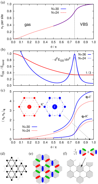
Figure 5: (a) Occupation of the triplet state within the honeycomb model parametrized as $E_{T}=\cos\vartheta$, $K=\sin\vartheta$. Presented for a hexagonal $24$-site cluster and rectangular $30$-site cluster. (b) Ground-state energy per bond $E_{\mathrm{GS}}$ measured by bonding-state energy $E_{\mathrm{bond}}$ (red) and the second derivative of $E_{\mathrm{GS}}$ with respect to $\vartheta$ revealing the quantum critical point (blue). (c) Correlations $\langle n_{b}n_{b}\rangle_{\boldsymbol{q}}$ of the bosons $b$ on the dual kagomé lattice. Size-dependent correlations at the characteristic vector $\boldsymbol{q}=K^{\prime}$ detect the VBS state. The insets show the correlations at $\vartheta=0.95\pi$ plotted in the extended Brillouin zone of the kagomé lattice at all momenta accessible when using the $24$- and $30$-site clusters, respectively. (d) Static pattern of the $b$ bosons on the dual lattice suggested by their reciprocal-space correlations. (e) Corresponding arrangement of $T$-dimers in the original representation. Red, green, and blue ellipses represent bonding states involving $T_{x}$, $T_{y}$, and $T_{z}$, respectively. The shaded hexagons indicate flippable plaquettes. (f) The actual plaquette order in VBS phase. The shaded hexagons indicate resonating plaquettes.

This similarity is seen already in Fig. 5(a),(b) which is a direct analogy of Fig. 3(a),(b) capturing the competition between the gas and VBS phase in the Kitaev-like limit of the model. Again a single QCP is detected, now with a position shifted to a smaller $K/|E_{T}|$ ratio in the negative $E_{T}$ region. The reduction of the VBS phase is a consequence of the lattice connectivity – the VBS state can only host a bonding state on one third of the bonds compared to one half in the chain case, leading to a less competitive energy gain. The formation of VBS consisting of maximum geometrically possible number of dimers (bonding states), i.e. $N_{\mathrm{bond}}/3$, is seen also in the GS energy per bond measured by $E_{\mathrm{bond}}$. This quantity stays close to $\frac{1}{3}$ and there is again a small positive deviation scaling as $K^{6}$ that indicates residual interactions among the dimers. They establish a specific dimer arrangement that we detect in Fig. 5(c) using dual $b$-boson representation on the kagomé lattice as described in Sec. III.2 (note that all the bond parities are even in the case inspected). The VBS phase is marked by size-dependent reciprocal-space correlations of the $b$-boson density $n_{b}$ at the characteristic momenta $\boldsymbol{q}=K^{\prime}$ lying in the corners of the extended Brillouin zone of the kagomé lattice. This suggests the real-space pattern shown in Fig. 5(d) that is also the most probable $b$ configuration in the ground state. Translating it into the $T$-dimer picture, we obtain the pattern in Fig. 5(e) which maximizes the number of plaquettes carrying three dimers. However, the true structure of the ground state is more complicated and requires the following deeper analysis.

In fact, working in the basis of maximum dimer coverings, an effective quantum dimer model (QDM) with $\mathcal{O}(K^{6})$ interactions can be formulated. This QDM “lives” in the all-even parity sector and captures both the ground state and the lowest excitations. Leaving the details aside, we note that the dimer model involves two kinds of interactions: First, there is an energy gain $\propto K^{6}$ from dimer-dimer bonds which is constant for all the coverings and which was already noticed in the 1D case with just two trivial dimer coverings. The second contribution, being the actual driving force stabilizing the VBS pattern, is enabled by the geometry of the honeycomb lattice and corresponds to hexagonal plaquette flips with an amplitude $\propto K^{6}$. They are captured by the QDM Hamiltonian

$$\mathcal{H}_{\mathrm{QDM}}=-t\sum_{\mathrm{plaquettes}}\left(\left|\raisebox{-6.0pt}{\includegraphics[height=18.0pt]{fig_plaquette1}}\right\rangle\left\langle\raisebox{-6.0pt}{\includegraphics[height=18.0pt]{fig_plaquette2}}\right|+\mathrm{H.c.}\right),$$ (27)

with $t=3K^{6}/16|E_{T}|^{5}$, i.e. by the kinetic term of the Rokhsar–Kivelson (RK) model for the honeycomb lattice [29; 30]. Using the connection to this well-studied model we can fix the type of order in the VBS phase now. The phase diagram of the honeycomb RK model, depending on the ratio of the flippable plaquette energy cost $V$ and the flipping amplitude $t$, was precisely determined by Monte Carlo simulations [30; 31; 32]. Our $V/t=0$ case falls into the interval between $(V/t)_{c}\approx-0.23$ [32] and the RK point $V/t=1$ where the honeycomb RK model supports a triangular covering by resonating plaquettes (“plaquette” order) depicted approximately in Fig. 5(f) which is the true VBS order for our model. The anticipated “columnar” order of Fig. 5(e) only appears below the (rather close) critical point $(V/t)_{c}$ of the RK model where the sufficiently large negative potential energy of the plaquettes wins.

Finally, we conclude the comparison to the Kitaev-like 1D model by a remark that the spin gap behavior for the honeycomb lattice strongly resembles that of the 1D chain case [see Fig. 3(c)], i.e. the spin gap gradually closes as we approach the QCP from both the gas as well as VBS phases.

V.2 Full honeycomb model

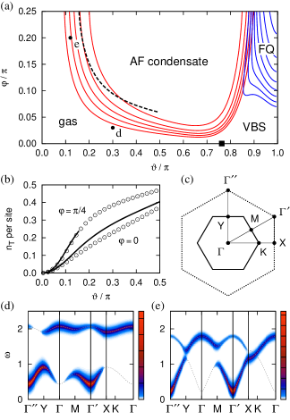
Figure 6: (a) Approximate phase diagram of $E_{T}-K-\tilde{K}$ model up to $\tilde{K}\!=\!K$ estimated as in Fig. 4(b) via size-dependent characteristic correlations. Hexagonal $6$-site cluster and rectangular $12$-site cluster were used. The model is parametrized as: $E_{T}=\cos\vartheta$, $K=\sin\vartheta\cos\varphi$, $\tilde{K}=\sin\vartheta\sin\varphi$. Red lines show contours of the increase of the van Vleck correlations $\langle S^{x}_{\boldsymbol{q}}S^{x}_{-\boldsymbol{q}}\rangle$ at the antiferromagnetic (AF) momentum $\boldsymbol{q}=\Gamma^{\prime}$ when going from $6$- to $12$-site cluster. The correlations detecting the ferroquadrupolar (FQ) phase (blue contours) were estimated as described in the text. Black square is the extrapolated position of the QCP for pure Kitaev-like ($K$ only) model [see Fig. 5(b)]. The dashed line indicates the transition between the gas phase and AF condensate obtained using Gutzwiller-type treatment of the hardcore constraint. (b) Comparison of mean-field (solid line) and ED results (circles, 12-site cluster) for $n_{T}$ at the top ($\varphi=\pi/4$) and bottom line ($\varphi=0$) of the phase diagram. (c) Brillouin zone of the honeycomb lattice (solid) and completed triangular lattice (dotted) with indicated special points and the path used in the next panels. (d),(e) Imaginary part of van Vleck spin susceptibility $\chi_{zz}(\boldsymbol{q},\omega)$ calculated in the mean-field approximation for the two points marked by d and e in panel (a) and artificially broadened. The dotted lines indicate the dispersions of Eq. (V.2.2) with $\alpha=z$.

In this section we explore the phase diagram and to a limited extent also the excitations of the full model of Eq. (10) containing both the Kitaev-like interaction $K$ and the complementary one $\tilde{K}$. We do not go up to the dominant $\tilde{K}$ regime characterized by strongly interacting quasi-one-dimensional condensates hosted by zigzag chains in the honeycomb lattice [12]. Instead, similarly to the chain case, we interpolate between the Kitaev-like limit and the isotropic limit $K=\tilde{K}$, being both positive as derived. Phase diagram for arbitrary $\tilde{K}/K$ ratio and positive $E_{T}>0$ sector can be found in Ref. [17].

V.2.1 Phase diagram

Fig. 6(a) presents the phase diagram of the $E_{T}-K-\tilde{K}$ model estimated by the method of Sec. IV.2, i.e. by tracking the cluster-size-dependent correlations characteristic to the individual phases. Due to a larger local basis of four states, lack of symmetries, and many points to be analyzed, we had to resort to a combination of small $6$-site and $12$-site clusters. This makes the phase diagram rather semi-quantitative as seen for example by comparing the position of the QCP in the Kitaev-like limit obtained for much bigger clusters in Sec. V.1. Nevertheless, four phases in an arrangement resembling that of Fig. 4(b) can be identified. Two of them – gas and VBS phases – were already encountered in the previous Sec. V.1.

The left part of the phase diagram ($E_{T}>0$) is a playground for a competition between the AF correlations and Kitaev-like frustration of the interactions. In the isotropic $K\!=\!\tilde{K}$ limit [top line in Fig. 6(a)] where the bond interactions handle all the triplon colors equally, the situation is analogous to the square-lattice case discussed in the context of Ca₂RuO₄ [12; 14; 15]. Since the honeycomb lattice is not geometrically frustrated, it can easily host an antiferromagnetic phase associated with a bipartite condensation of triplons captured by a wavefunction similar to that of Eq. (23). This AF phase with “soft” (i.e. far from saturated) van Vleck moments $\boldsymbol{M}_{1}$ actually takes the largest portion of the entire phase diagram in Fig. 6(a). Going down to the region with strong Kitaev-like anisotropy of the interactions and the resulting frustration, the AF phase gets largely suppressed. One of the highlights of the soft-moment magnetism based on spin-orbit triplon condensation is the presence of both transverse magnon modes as well as an intense amplitude mode (dubbed “Higgs mode” in this context), that have been observed experimentally in Ca₂RuO₄ [14; 15]. It is an interesting and non-trivial problem for a future study to analyze the effect of the Kitaev-like frustration on such magnetic excitation spectra. Later in Sec. V.2.2, we only make an attempt to address the gas phase close to the AF phase boundary, by inspecting the excitation spectrum close to the point where the condensate is formed.

Focusing now on the large negative $E_{T}$ limit, we can again notice similarities to the 1D chain case of Sec. IV.2. In this limit the singlets $s$ can be integrated out leaving us with an effective spin-1 model where the spin now coincides with the triplon spin $-i(\boldsymbol{T}^{\dagger}\times\boldsymbol{T})$. The nature of this model changes with the $\tilde{K}/K$ ratio. For the strongly anisotropic $K$-only case, one formally obtains a biquadratic Kitaev-like model as a leading term:

$$\mathcal{H}_{\mathrm{bqK}}=-\frac{K^{2}}{2|E_{T}|}\,\sum_{\langle ij\rangle}(S^{\alpha}_{i}S^{\alpha}_{j})^{2},$$ (28)

with the active component $\alpha\in\{x,y,z\}$ given by the bond direction as before. Compared to the usual bilinear spin-one Kitaev model (see, e.g., Ref. [33] and references therein), the behavior of the biquadratic model is rather trivial. In the original language, it simply counts the number of proper-color $T$-dimers and associates an energy gain ${K^{2}}/2|E_{T}|$ with each of them. This selects a large number of degenerate $T$-dimer coverings as the model ground state. At this level of approximation which misses the $\mathcal{O}(K^{6})$ interactions, the true VBS ground state cannot be resolved. Furthermore, the low-lying excitations with the energies $\propto K^{6}$ are not captured. Hence, in the Kitaev-like limit, spin-1 is not a suitable elementary object and bonding-state dimers should be used instead, leading to the effective quantum dimer model which we extensively discussed in Sec. V.1.

In contrast to that, the isotropic limit $K\!=\!\tilde{K}$ can be expected to be adequately captured by a simple isotropic spin-1 model. Indeed, the preference of the total-singlet $T$-pairs that may virtually transform into $s$-pairs and back gives rise to biquadratic interaction described by the effective Hamiltonian

$$\mathcal{H}_{\mathrm{bq}}=-\frac{K^{2}}{2|E_{T}|}\,\sum_{\langle ij\rangle}(\boldsymbol{S}_{i}\boldsymbol{S}_{j})^{2}$$ (29)

at the isotropic point $K\!=\!\tilde{K}$. Model of this kind is a special case of bilinear-biquadratic spin-1 models that were thoroughly explored for various lattices. On a non-bipartite, geometrically frustrated triangular lattice [34; 35] its ground state shows a ferroquadrupolar (FQ) order [36; 37; 38] which does not break time-reversal symmetry but introduces a preferential plane in spin space where the spins can be found with a higher probability. For a non-frustrated lattice such as square [37; 39] and honeycomb [40; 41; 42] the AF phase is more competitive and the biquadratic model is just on the verge of the FQ and AF order. This type of order, labeled as FQ in Fig. 6(a) for simplicity, therefore replaces the Bethe phase of the 1D chain [compare Fig. 4(b)]. Note that here we refer to the AF phase of triplon spins $-i(\boldsymbol{T}^{\dagger}\times\boldsymbol{T})$; this should not be confused with the neighboring AF phase of correlated van Vleck moments $\boldsymbol{M}_{1}$ which reside on the $J=0\leftrightarrow 1$ transitions. The detection of the “edge-case” FQ/AF order is somewhat complicated, also due to the incompatible geometry of the two clusters ($6$-site hexagon and $12$-site rectangle) that we use to check the size-scaling of the characteristic correlations. To this end, as the characteristic quantity we take the contribution to FQ correlations $\langle Q_{\boldsymbol{q}}Q_{-\boldsymbol{q}}\rangle$ with $\boldsymbol{q}=0$ that is carried by triplon spins at AF momentum $\boldsymbol{q}=\Gamma^{\prime}$. More explicitly, we decompose the various quadrupole operators $Q$ containing $S^{\alpha}S^{\beta}$ terms (see e.g. Ref. [34] for their explicit forms) into a momentum sum $Q_{\boldsymbol{q}}\sim\sum_{\boldsymbol{q}^{\prime}}S_{\boldsymbol{q}-\boldsymbol{q}^{\prime}}^{\alpha}S_{\boldsymbol{q}^{\prime}}^{\beta}$ and evaluate the four-spin correlators of the type $\langle S_{\boldsymbol{q}-\boldsymbol{q}^{\prime}}^{\alpha}S_{\boldsymbol{q}^{\prime}}^{\beta}S_{-\boldsymbol{q}-\boldsymbol{q}^{\prime\prime}}^{\gamma}S_{\boldsymbol{q}^{\prime\prime}}^{\delta}\rangle$ constituting $\langle Q_{\boldsymbol{q}}Q_{-\boldsymbol{q}}\rangle$. The contribution with all the momenta being equal to the AF one is found to dominate and behave well at the reference $K=\tilde{K}\ll|E_{T}|$ point described by $\mathcal{H}_{\mathrm{bq}}$ of Eq. (29). The resulting correlations obtained as a difference between 12-site and 6-site cluster are shown in Fig. 6(a). They suggest that FQ/AF phase extends slightly further from its reference point than the VBS one, though this result may be potentially biased as the small clusters can not properly accommodate the VBS state. As a general remark on biquadratic spin models such as (29), it is worth noticing that while they are typically very weak in conventional spin systems, they emerge naturally in singlet-triplet level systems; see yet another example in Ref. [43].

V.2.2 Dynamical Gutzwiller treatment and excitations

As argued in Sec. III.3, the Kitaev-like anisotropy of the interactions should manifest itself by the localized nature of the dynamic spin response which translates to the flat dispersions of the spin excitations. Having now covered the entire interval from the Kitaev-like limit to the isotropic limit, one might wonder about the corresponding evolution of the spin excitations. Due to the limited cluster size, ED calculations do not provide a sufficient resolution to study such effects.

Here we adopt instead a dynamical Gutzwiller treatment combined with selfconsistent mean-field approximation formulated for the triplon gas phase. Besides the excitation spectrum, this enables us to obtain the gas/AF transition point as a function of non-Kitaev term $\tilde{K}$. The derivation starts with a replacement of $s$ implicitly contained in Eq. (10) by the operator $\sqrt{1-n_{T}}$ which dynamically accounts for the triplon hardcore constraint. The resulting Hamiltonian is expanded and a mean-field decoupling is applied leading to the quadratic Hamiltonian

$$\mathcal{H}_{\mathrm{MF}}=\sum_{i}(E_{T}+\Lambda)\,n_{T_{i}}\\ +\sum_{{\langle ij\rangle}_{\alpha}}\langle 1-n_{T}\rangle[K\mathcal{O}_{ij}^{\alpha}+\tilde{K}(\mathcal{O}_{ij}^{\bar{\alpha}}+\mathcal{O}_{ij}^{\bar{\bar{\alpha}}})],$$ (30)

where all the $s$, $s^{\dagger}$ operators in $\mathcal{O}$ are left out. At this point we have already relaxed the hardcore constraint. Two effects of the hardcore nature of the triplons got captured at the level of $\mathcal{H}_{\mathrm{MF}}$: (i) effective triplon cost is increased by an energy

$$\Lambda=-\frac{1}{2}\sum_{\delta_{\alpha}}\bigl{[}K\langle\mathcal{O}_{i,i+\delta}^{\alpha}\rangle+\tilde{K}(\langle\mathcal{O}_{i,i+\delta}^{\bar{\alpha}}\rangle+\langle\mathcal{O}_{i,i+\delta}^{\bar{\bar{\alpha}}}\rangle)\bigr{]}$$ (31)

($\delta$ runs through all nearest-neighbors), and (ii) the interactions $K$, $\tilde{K}$ are reduced by a factor $1-\langle n_{T}\rangle$ that embodies the probability of another triplon blocking the interaction process on the particular bond. After a conversion to momentum space we obtain

$$\mathcal{H}_{\mathrm{MF}}=\sum_{\boldsymbol{k}\alpha}E\,\bigl{(}\alpha_{1\boldsymbol{k}}^{\dagger}\alpha_{1\boldsymbol{k}}^{\phantom{\dagger}}+\alpha_{2\boldsymbol{k}}^{\dagger}\alpha_{2\boldsymbol{k}}^{\phantom{\dagger}}\bigr{)}\\ +\Bigl{[}\kappa_{\alpha\boldsymbol{k}}\bigl{(}\alpha_{1\boldsymbol{k}}^{\dagger}\alpha_{2\boldsymbol{k}}^{\phantom{\dagger}}-\alpha_{1,-\boldsymbol{k}}^{\phantom{\dagger}}\alpha_{2\boldsymbol{k}}^{\phantom{\dagger}}\bigr{)}+\mathrm{H.c.}\Bigr{]},$$ (32)

where the unconstrained triplons are labeled by their color $\alpha=x,y,z$ and the index $1$ or $2$ referring to the two sites in the unit cell of the honeycomb lattice. It is convenient to choose the unit cell for triplons of color $\alpha$ as a bond of direction $\alpha$. In this convention, the on-site triplon energy $E=E_{T}+\Lambda$ entering Eq. (32) is complemented by the interaction term $\kappa_{\alpha\boldsymbol{k}}=\langle 1-n_{T}\rangle(K+\tilde{K}\eta_{\alpha\boldsymbol{k}})$ with the formfactor $\eta_{z\boldsymbol{k}}$ given by $\eta_{z\boldsymbol{k}}=2\cos(\frac{\sqrt{3}}{2}k_{x})\exp(-i\frac{3}{2}k_{y})$, and $\eta_{x\boldsymbol{k}}$ and $\eta_{y\boldsymbol{k}}$ being simply rotated by multiples of $2\pi/3$. Note that $\kappa_{\alpha\boldsymbol{k}}$ depends on momentum $k$ via non-Kitaev $\tilde{K}$-term only.

The $4\times 4$ problem contained in Eq. (32) can be diagonalized explicitly and yields the dispersions of the bosonic quasiparticles

$$\omega_{B\alpha\boldsymbol{k}} =\sqrt{E(E-2|\kappa_{\alpha\boldsymbol{k}}|)},$$

$$\quad\omega_{A\alpha\boldsymbol{k}} =\sqrt{E(E+2|\kappa_{\alpha\boldsymbol{k}}|)}.$$ (33)

The averages entering all the equations starting from Eq. (30) have to be calculated self consistently via

$$\langle n_{T}\rangle =\frac{1}{4}\sum_{\boldsymbol{k}\alpha}\left(\frac{E-|\kappa_{\alpha\boldsymbol{k}}|}{\omega_{B\alpha\boldsymbol{k}}}+\frac{E+|\kappa_{\alpha\boldsymbol{k}}|}{\omega_{A\alpha\boldsymbol{k}}}-2\right),$$ (34)

$$\Lambda =\frac{1}{4}\sum_{\boldsymbol{k}\alpha}|K+\tilde{K}\eta_{\alpha\boldsymbol{k}}|\left(\frac{E}{\omega_{B\alpha\boldsymbol{k}}}-\frac{E}{\omega_{A\alpha\boldsymbol{k}}}\right).$$ (35)

The above approach is applicable through the entire gas phase where the excitations are found to be gapped ($\omega_{B\alpha\boldsymbol{k}}$ and $\omega_{A\alpha\boldsymbol{k}}>0$). Once the lower-energy $\omega_{B\alpha\boldsymbol{k}}$ touches zero at some point of the Brillouin zone, the triplon condensation occurs with the condensate structure being similar to the one of Eq. (23). The corresponding condition $E=2|\kappa_{\alpha\boldsymbol{k}}|$ is first met at $\boldsymbol{k}=0$ which results in the following equation:

$$E_{T}+\Lambda=2\langle 1-n_{T}\rangle(K+2\tilde{K})$$ (36)

determining the points where AF condensate starts to form. The gas/AF phase boundary obtained this way is presented as a dashed line in Fig. 6(a). It shows a good overall agreement with the estimate by ED, correctly capturing the physical trend of a delayed condensation when the frustration increases approaching the Kitaev-like limit. As expected, the best agreement is obtained near the isotropic limit which is also illustrated in Fig. 6(b) where the isotropic-limit data ($\varphi=\pi/4$) of the selfconsistent $\langle n_{T}\rangle$ perfectly match the ED values. In the Kitaev-like limit ($\varphi=0$), the deviation is already significant but still acceptable for our semi-quantitative analysis.

With an adequate description of the excitations in the gas phase at hand, we are now ready to inspect an analogy to Fig. 4(c),(d) presenting the dynamical spin susceptibility for the gas phase of the 1D chain model. To this end we express the Fourier component of the van Vleck moment operator $\propto-i(s^{\dagger}T^{\phantom{\dagger}}_{\alpha}-T^{\dagger}_{\alpha}s)$ in terms of the unconstrained triplons as

$$S^{\alpha}_{\boldsymbol{q}}\propto-i\left[\alpha_{1\boldsymbol{q}}^{\phantom{\dagger}}-\alpha_{1,-\boldsymbol{q}}^{\dagger}+(\alpha_{2\boldsymbol{q}}^{\phantom{\dagger}}-\alpha_{2,-\boldsymbol{q}}^{\dagger})\mathrm{e}^{-i\boldsymbol{q}\cdot\boldsymbol{\delta}_{\alpha}}\right],$$ (37)

where $\boldsymbol{\delta}_{\alpha}$ is a unit vector in the direction of $\alpha$ bonds. Next, we use the eigenspectrum of $\mathcal{H}_{\mathrm{MF}}$ to find the dynamic correlation function $\chi_{\alpha\alpha}(\boldsymbol{q},\omega)=\langle S^{\alpha}_{\boldsymbol{q}}S^{\alpha}_{-\boldsymbol{q}}\rangle_{\omega}$ shown in Fig. 6(d),(e) for two selected points in the phase diagram.

Similarly to the chain case, the vicinity of the Kitaev-like limit [Fig. 6(d)] is characterized by flat dispersion of excitations with the modulation being generated by nonzero $\tilde{K}$ only as it is evident from Eq. (V.2.2) and the form of $\kappa_{\alpha\boldsymbol{k}}$. Flat dispersions are the fingerprints of underlying frustrations, and resemble the Kitaev-Heisenberg model magnons characterized by two different energy scales [44]. The excitations in Eq. (V.2.2) have two branches for each triplon color $\alpha$ that cover the entire Brillouin zone associated with the completed triangular lattice [dotted hexagon in Fig. 6(c)] by periodic copies of the smaller Brillouin zone of the honeycomb lattice [full hexagon in Fig. 6(c)]. The intensity of these excitations in the dynamic spin susceptibility varies through the Brillouin zone – while the upper branch dominates around the $\boldsymbol{q}=\Gamma$ point, the lower branch is most intense around the AF wavevector $\boldsymbol{q}=\Gamma^{\prime}$. At the latter point (equivalent to $\boldsymbol{q}=\Gamma=0$ in terms of the bosonic excitations), the magnetic excitations will eventually touch zero energy signaling the transition into long-range AF phase as $\tilde{K}$ increases. This is also observed near the isotropic limit [see Fig. 6(e)] where the modulation of the originally flat dispersions by the complementary interaction $\tilde{K}$ leads to a merging of the two excitation branches and the result starts to resemble the excitonic magnon dispersion. In contrast to the Heisenberg model at the same lattice, it is characterized by a maximum at $\Gamma$ point, as has been seen experimentally in the square-lattice case of Ca₂RuO₄ [14].

The observed features of the presented gas-phase spectra close to the AF transition are expected to be already quite indicative for the AF phase. After the condensation, an additional excitation branch corresponding to the amplitude (Higgs) mode will develop [a hint of this can be noticed in the chain case when comparing Fig. 4(d) and (g)]. Besides that, there will be also an ongoing redistribution of the spectral weight in the magnon branch.

VI Conclusions

We have studied singlet-triplet models that describe magnetism of spin-orbit coupled $d^{4}$ Mott insulators, such as ruthenium Ru⁴⁺ or iridium Ir⁵⁺ compounds. Singlet-triplet models appear in various physical contexts (see, e.g., Refs. [22; 45; 46; 43]) and are of general interest because they host – by very construction – a quantum phase transition from triplon gas to the ordered state of soft moments, when exchange interactions overcome a singlet-triplet spin gap. The models considered here bring a new feature into this physics: a magnetic frustration that originates from bond-directional nature of orbital interactions [5]. Similar to the case of spin-orbit pseudospin $J=1/2$ Mott insulators with bond-directional Ising couplings [8; 9; 10; 11] on a honeycomb lattice, the orbital frustration has a strong impact on magnetism of singlet-triplet models [12; 17].

The main aim of the present work was to understand how a triplon gas evolves into a dense system of strongly interacting particles, in particular when bond-directional anisotropy of the exchange interactions are taken to the extreme as in Kitaev model. We find that this evolution is continuous and results in a strongly correlated paramagnet smoothly connected to a triplon gas. Even though this paramagnet misses the defining features of genuine spin-liquids (many-body entanglement and emergent quasiparticles) [2], it is far from being trivial. In contrast to a conventional O(3) singlet-triplet systems, spin correlations here are highly anisotropic and strictly short-ranged even in the limit of strong exchange interactions where the spin gap is very small. As in the Kitaev model, these peculiar features of spin correlations follow from the symmetry properties of the model – an extensive number of conserved $Z_{2}$ quantities that decompose the Hilbert space into subspaces with fixed bond-parity configurations. We have also shown that the model can be mapped to a bilayer version of Kitaev model, but with some additional terms in the interlayer couplings which act to suppress gas-to-liquid phase transition in a bilayer Kitaev model [18; 19; 20]. Exact diagonalization of the model in 1D-zigzag chain as well as on honeycomb lattice show that the lowest energy excitations are in the spin sector (and always gapped). This is different from the Kitaev model with Majorana bands within the spin gap.

Going away from Kitaev-like symmetry of the exchange interactions towards isotropic O(3) limit, we find that triplons condense into AF ordered phase at finite critical value of non-Kitaev $\tilde{K}$ term. At $\tilde{K}<K$ regime (and close to phase transition), spin excitations show two distinct branches of weakly dispersive modes [Fig. 6(d)]; however, this result is obtained within a mean-field treatment of the hard-core constraint neglecting any multi-particle scattering processes. A quantitative description of the highly frustrated magnetic condensate and its excitations in the regime of $\tilde{K}<K$ remains an open theoretical problem.

Considering the model at negative $E_{T}$ values, we observe the links to some exotic models such as biquadratic spin-1 and quantum dimer models. At negative $E_{T}$ and small $\tilde{K}$ regime, we find a quantum phase transition from strongly correlated paramagnetic phase to a plaquette-VBS state of the triplon-dimers.

Apart from a theoretical interest in frustrated singlet-triplet models, this study was partly motivated by magnetic properties of honeycomb lattice ruthenium compounds, in particular Ag₃LiRu₂O₆ [47; 48; 49]. This compound is derived from Li₂RuO₃ by substituting Ag-ions for those Li-ions which reside between the Ru-honeycomb planes. As a result, a structural transition observed in Li₂RuO₃ [16] is completely suppressed, suggesting Ag₃LiRu₂O₆ as a nearly ideal honeycomb lattice system to study the interplay between spin-orbit coupling and exchange interactions. Current data [47; 48; 49] shows that this compound is insulating and has no magnetic order, which would be consistent with the (correlated) triplon-gas phase where interactions are either too weak to overcome the spin-orbit gap, or they are strongly frustrated preventing triplon condensation. As $4d$-electron wavefunctions are rather extended in space, a direct overlap processes can be sizable in ruthenates [50], thus raising the possibility of bond-directional triplon dynamics in this material. Future experiments probing magnetic dynamics are necessary to identify symmetry of the dominant exchange interactions in Ag₃LiRu₂O₆. Metallic states induced by electron doping of this material could bring some surprises as well.

Overall, the orbitally frustrated singlet-triplet models show a rich physics, interesting theoretically and also relevant to spin-orbit coupled $J_{\mathrm{eff}}=0$ Mott insulators based on, e.g., ruthenium Ru⁴⁺ and iridium Ir⁵⁺ ions.

- [1] L. Balents, Nature (London) 464, 199 (2010).
- [2] L. Savary and L. Balents, Rep. Prog. Phys. 80, 016502 (2017).
- [3] M. Vojta, Rep. Prog. Phys. 81, 064501 (2018).
- [4] K. I. Kugel and D. I. Khomskii, Sov. Phys. Usp. 25, 231 (1982).
- [5] G. Khaliullin, Prog. Theor. Phys. Suppl. 160, 155 (2005).
- [6] Z. Nussinov and J. van den Brink, Rev. Mod. Phys. 87, 1 (2015).
- [7] A. Kitaev, Ann. Phys. 321, 2 (2006).
- [8] G. Jackeli and G. Khaliullin, Phys. Rev. Lett. 102, 017205 (2009).
- [9] J. Chaloupka, G. Jackeli, and G. Khaliullin, Phys. Rev. Lett. 105, 027204 (2010).
- [10] H. Liu and G. Khaliullin, Phys. Rev. B 97, 014407 (2018).
- [11] R. Sano, Y. Kato, and Y. Motome, Phys. Rev. B 97, 014408 (2018).
- [12] G. Khaliullin, Phys. Rev. Lett. 111, 197201 (2013).
- [13] O. N. Meetei, W. S. Cole, M. Randeria, and N. Trivedi, Phys. Rev. B 91, 054412 (2015).
- [14] A. Jain, M. Krautloher, J. Porras, G. H. Ryu, D. P. Chen, D. L. Abernathy, J. T. Park, A. Ivanov, J. Chaloupka, G. Khaliullin, B. Keimer, and B. J. Kim, Nature Phys. 13, 633 (2017).
- [15] S.-M. Souliou, J. Chaloupka, G. Khaliullin, G. Ryu, A. Jain, B. J. Kim, M. Le Tacon, and B. Keimer, Phys. Rev. Lett. 119, 067201 (2017).
- [16] Y. Miura, Y. Yasui, M. Sato, N. Igawa, and K. Kakurai, J. Phys. Soc. Jpn. 76, 033705 (2007).
- [17] P. S. Anisimov, F. Aust, G. Khaliullin, and M. Daghofer, Phys. Rev. Lett. 122, 177201 (2019).
- [18] H. Tomishige, J. Nasu, and A. Koga, Phys. Rev. B 97, 094403 (2018).
- [19] U. F. P. Seifert, J. Gritsch, E. Wagner, D. G. Joshi, W. Brenig, M. Vojta, and K. P. Schmidt, Phys. Rev. B 98, 155101 (2018).
- [20] H. Tomishige, J. Nasu, and A. Koga, Phys. Rev. B 99, 174424 (2019).
- [21] X-F. Zhang, Y-C. He, S. Eggert, R. Moessner, and F. Pollmann, Phys. Rev. Lett. 120, 115702 (2018).
- [22] T. Giamarchi, Ch. Rüegg, and O. Tchernyshyov, Nat. Phys. 4, 198 (2008).
- [23] C. E. Agrapidis, J. van den Brink, and S. Nishimoto, Sci. Rep. 8, 1815 (2018).
- [24] R. Botet, R. Jullien, and M. Kolb, Phys. Rev. B 28, 3914 (1983).
- [25] H. J. Schulz, Phys. Rev. B 34, 6372 (1986).
- [26] M. den Nijs and K. Rommelse, Phys. Rev. B 40, 4709 (1989).
- [27] W. Chen, K. Hida, and B. C. Sanctuary, Phys. Rev. B 67, 104401 (2003).
- [28] A. Langari, F. Pollmann, and M. Siahatgar, J. Phys.: Condens. Matter 25, 406002 (2013).
- [29] D. S. Rokhsar and S. A. Kivelson, Phys. Rev. Lett. 61, 2376 (1988).
- [30] R. Moessner, S. L. Sondhi, and P. Chandra, Phys. Rev. B 64, 144416 (2001).
- [31] T. Schlittler, T. Barthel, G. Misguich, J. Vidal, and R. Mosseri, Phys. Rev. Lett. 115, 217202 (2015).
- [32] T. M. Schlittler, R. Mosseri, and T. Barthel, Phys. Rev. B 96, 195142 (2017).
- [33] T. Minakawa, J. Nasu, A. Koga, arXiv:1909.10170.
- [34] A. Läuchli, F. Mila, and K. Penc, Phys. Rev. Lett. 97, 087205 (2006).
- [35] H. Tsunetsugu and M. Arikawa, J. Phys. Soc. Jpn. 75, 083701 (2006).
- [36] H. H. Chen and P. M. Levy, Phys. Rev. B 7, 4267 (1973).
- [37] K. Harada and N. Kawashima, Phys. Rev. B 65, 052403 (2002).
- [38] B. A. Ivanov and A. K. Kolezhuk, Phys. Rev. B 68, 052401 (2003).
- [39] T. A. Tóth, A. M. Läuchli, F. Mila, and K. Penc, Phys. Rev. B 85, 140403(R) (2012).
- [40] Y.-W. Lee and M.-F. Yang, Phys. Rev. B 85 100402(R) (2012).
- [41] H. H. Zhao, C. Xu, Q. N. Chen, Z. C. Wei, M. P. Qin, G. M. Zhang, and T. Xiang, Phys. Rev. B 85, 134416 (2012).
- [42] P. Corboz, M. Lajkó, K. Penc, F. Mila, and A. M. Läuchli, Phys. Rev. B 87, 195113 (2013).
- [43] J. Chaloupka and G. Khaliullin, Phys. Rev. Lett. 110, 207205 (2013).
- [44] J. Chaloupka, G. Jackeli, and G. Khaliullin, Phys. Rev. Lett. 110, 097204 (2013).
- [45] T. Sommer, M. Vojta, and K. W. Becker, Eur. Phys. J. B 23, 329 (2001).
- [46] G. Chen, L. Balents, and A. P. Schnyder, Phys. Rev. Lett. 102, 096406 (2009).
- [47] S. A. J. Kimber, C. D. Ling, D. J. P. Morris, A. Chemseddine, P. F. Henry, and D. N. Argyriou, J. Mater. Chem. 20, 8021 (2010).
- [48] R. Kumar, T. Dey, P. M. Ette, K. Ramesha, A. Chakraborty, I. Dasgupta, J. C. Orain, C. Baines, S. Tóth, A. Shahee, S. Kundu, M. Prinz-Zwick, A. A. Gippius, N. Büttgen, P. Gegenwart, and A. V. Mahajan, Phys. Rev. B 99, 054417 (2019).
- [49] T. Takayama et al. (unpublished).
- [50] S. V. Streltsov and D. I. Khomskii, Phys.-Usp. 60, 1121 (2017).