Large Intelligent Surface for Positioning in Millimeter Wave MIMO Systems

Abstract

Millimeter-wave (mmWave) multiple-input multiple-output (MIMO) system for the fifth generation (5G) cellular communications can also enable single-anchor positioning and object tracking due to its large bandwidth and inherently high angular resolution. In this paper, we introduce the newly invented concept, large intelligent surface (LIS), to mmWave positioning systems, study the theoretical performance bounds (i.e., Cramér-Rao lower bounds) for positioning, and evaluate the impact of the number of LIS elements and the value of phase shifters on the position estimation accuracy compared to the conventional scheme with one direct link and one non-line-of-sight path. It is verified that better performance can be achieved with a LIS from the theoretical analyses and numerical study.

I Introduction

Conventionally, indoor and outdoor positioning is carried out by using received signal strength (RSS), time-difference-of-arrival (TDoA) [1] or fingerprinting-based approaches [2, 3]. Recently, efforts on positioning has been made by leveraging millimeter-wave (mmWave) multiple-input multiple-output (MIMO) systems and the geometric relationship between the base station (BS) and the mobile station (MS) [4, 5, 6, 7, 8]. It was shown that even a single BS can achieve promising positioning accuracy. Extensions to multiple-carrier and multi-user scenarios were studied in [7].

Practical positioning algorithms for the single-anchor mmWave MIMO system can be classified into two major categories, i.e., direct positioning [6] and two-stage positioning [4, 5, 7, 8]. The direct positioning aims at estimating the coordinates of the MS from the received signal directly, while the two-stage positioning first estimates the instantaneous channel realization: the channel gains, the angle of departure (AoD), the angle of arrival (AoA), and the time of arrival (ToA). In the second stage, the user location is calculated based on the channel estimates and the environmental geometry.

Large intelligent surfaces (LIS), also known as reconfigurable intelligent surfaces (RIS), can effectively control the propagation wave, e.g., phase and even amplitude, without any need of baseband processing units [9, 10]. The LIS has been proposed to be used as a Tx/Rx antenna like in hybrid beamforming for positioning [11] and relay type reflector for communications [9].

In this paper, we study the positioning with the assistance of a LIS based reflector and multiple subcarriers at mmWave frequency bands. First, the performance bounds (i.e., Cramér-Rao lower bound) are evaluated based on the equivalent Fisher information matrix (FIM). The impact of the LIS, e.g., phase shifter value and the number of LIS elements, is studied on the estimation of channel parameters, positioning error bound (PEB), and orientation error bound (OEB). Numerical results show the superiority of the LIS aided mmWave MIMO positioning system over its conventional counterpart without incorporating a LIS.

II System Model

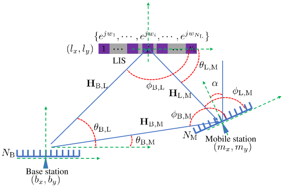
Figure 1: Positioning system with the aid of a large intelligent surface and multi-carrier mmWave OFDM signals. The coordinates and orientation of MS, $(m_{x},m_{y})$ and $\alpha$, are unknown and to be estimated.

The positioning system is presented in Fig. 1, which consists of one multiple-antenna BS, one multiple-antenna MS and one LIS. We consider a two-dimensional (2D) scenario with uniform linear arrays (ULAs) for both the antenna elements and LIS elements (i.e., analog phase shifters). The numbers of antenna elements at the BS and MS are $N_{\text{B}}$ and $N_{\text{M}}$, respectively, while the number of LIS elements is $N_{\text{L}}$. No rotation is assumed for the BS and the LIS while $\alpha$-rad rotation is assumed for the MS. The objective of the system is to localize the MS and estimate its orientation by using the received signals at the MS with $N$ mmWave orthogonal frequency division multiplexing (OFDM) subcarriers.

The propagation channel is composed of one direct path and one reflection path via the LIS. The direct channel between the BS and MS for the $n$-th subcarrier is expressed as

$${\mathbf{H}}_{\text{B,M}}[n] =\rho_{\text{B,M}}e^{-j2\pi\tau_{\text{B,M}}\frac{nB}{N}}\boldsymbol{\alpha}_{r}(\phi_{\text{B,M}})\boldsymbol{\alpha}_{t}^{H}(\theta_{\text{B,M}}),$$

$$\;\;\text{for}\;n=-(N-1)/2,\cdots,(N-1)/2,$$ (1)

where $\boldsymbol{\alpha}_{r}(\phi_{\text{B,M}})\in\mathbb{C}^{N_{\text{M}}\times 1}$ and $\boldsymbol{\alpha}_{t}(\theta_{\text{B,M}})\in\mathbb{C}^{N_{\text{B}}\times 1}$ are the antenna array response and steering vectors at the MS and BS, respectively. The $i$-th entry of $\boldsymbol{\alpha}_{r}(\phi_{\text{B,M}})$ and $\boldsymbol{\alpha}_{t}(\theta_{\text{B,M}})$ are $[\boldsymbol{\alpha}_{r}(\phi_{\text{B,M}})]_{i}=e^{j2\pi(i-1)\frac{d}{\lambda}\sin(\phi_{\text{B,M}})}$, $[\boldsymbol{\alpha}_{t}(\theta_{\text{B,M}})]_{i}=e^{j2\pi(i-1)\frac{d}{\lambda}\sin(\theta_{\text{B,M}})}$ with $d$ being the antenna element spacing, $\lambda$ being the wavelength of the signal, and $\theta_{\text{B,M}}$ and $\phi_{\text{B,M}}$ being the AoD and AoA, respectively. $j=\sqrt{-1}$, $\tau_{\text{B,M}}$ is the ToA, $B$ is the overall bandwidth for all the subcarriers, and $B\ll f_{c}$, where $f_{c}$ is the center frequency. $\rho_{\text{B,M}}\in\mathbb{R}^{+}$ is the free-space path loss occurred in the direct link for all the subcarriers, and $(\cdot)^{H}$ denotes the conjugate transpose operation.

The two tandem channels (${\mathbf{H}}_{\text{B,L}}[n]\in\mathbb{C}^{N_{\text{L}}\times N_{\text{B}}}$ for the first hop and ${\mathbf{H}}_{\text{L,M}}[n]\in\mathbb{C}^{N_{\text{M}}\times N_{\text{L}}}$ for the second hop) for the $n$-th subcarrier, which connect the BS to the MS via the LIS, are defined as

$${\mathbf{H}}_{\text{B,L}}[n]=\rho_{\text{B,L}}e^{-j2\pi\tau_{\text{B,L}}\frac{nB}{N}}\boldsymbol{\alpha}_{r}(\phi_{\text{B,L}})\boldsymbol{\alpha}_{t}^{H}(\theta_{\text{B,L}}),$$ (2)

and

$${\mathbf{H}}_{\text{L,M}}[n]=\rho_{\text{L,M}}e^{-j2\pi\tau_{\text{L,M}}\frac{nB}{N}}\boldsymbol{\alpha}_{r}(\phi_{\text{L,M}})\boldsymbol{\alpha}_{t}^{H}(\theta_{\text{L,M}}),$$ (3)

where the notations $\boldsymbol{\alpha}_{t}(\theta_{\text{B,L}})$, $\boldsymbol{\alpha}_{r}(\phi_{\text{B,L}})$, $\boldsymbol{\alpha}_{t}(\theta_{\text{L,M}})$, $\boldsymbol{\alpha}_{r}(\phi_{\text{L,M}})$, $\rho_{\text{B,L}}$, $\rho_{\text{L,M}}$, $\tau_{\text{B,L}}$, and $\tau_{\text{L,M}}$ are defined in the same way as those in (II).

The entire channel, including both the line-of-sight (LoS) path and the non-line-of-sight (NLoS) path (i.e., the reflection path via the LIS), between the BS and the MS for the $n$-th subcarrier can be formulated as

$${\mathbf{H}}[n]={\mathbf{H}}_{\text{B,M}}[n]+{\mathbf{H}}_{\text{L,M}}[n]\boldsymbol{\Omega}{\mathbf{H}}_{\text{B,L}}[n],$$ (4)

where $\boldsymbol{\Omega}=\mathrm{diag}(\exp\{j\omega_{1}\},\cdots,\exp\{j\omega_{N_{\text{L}}}\})\in\mathbb{C}^{N_{\text{L}}\times N_{\text{L}}}$ is the phase control matrix at the LIS. It is a diagonal matrix with constant-modulus entries in the diagonal.

Assuming that precoding ${\mathbf{F}}$ is exploited at the BS and the positioning reference signal (PRS) ${\mathbf{x}}[n]$ is transmitted over the $n$-th subcarrier, the downlink received signal is in the form of

$${\mathbf{y}}[n]=\sqrt{P}{\mathbf{H}}[n]{\mathbf{F}}{\mathbf{x}}[n]+{\mathbf{n}}[n],$$ (5)

where each entry in the additive white noise ${\mathbf{n}}[n]$ follows circularly-symmetric complex normal distribution $\mathcal{CN}(0,2\sigma^{2})$, and $P$ is the transmit power of the PRS.

The geometric relationship among the BS, LIS, and MS is formulated as

$$\tau_{\text{B,M}}=\|{\mathbf{b}}-{\mathbf{m}}\|_{2}/c,$$

$$\tau_{\text{B,L}}+\tau_{\text{L,M}}=\|{\mathbf{b}}-{\mathbf{l}}\|_{2}/c+\|{\mathbf{m}}-{\mathbf{l}}\|_{2}/c,$$

$$\theta_{\text{B,M}}=\arccos((m_{x}-b_{x})/\|{\mathbf{b}}-{\mathbf{m}}\|_{2}),$$

$$\theta_{\text{B,L}}=\arccos((l_{x}-b_{x})/\|{\mathbf{l}}-{\mathbf{b}}\|_{2}),$$

$$\theta_{\text{L,M}}=-\arccos((m_{x}-l_{x})/\|{\mathbf{l}}-{\mathbf{m}}\|_{2}),$$

$$\phi_{\text{B,M}}=\pi+\arccos((m_{x}-b_{x})/\|{\mathbf{b}}-{\mathbf{m}}\|_{2})-\alpha$$

$$\;\;\;\;\;\;=\pi+\theta_{\text{B,M}}-\alpha,$$

$$\phi_{\text{B,L}}=-\pi+\arccos((l_{x}-b_{x})/\|{\mathbf{b}}-{\mathbf{l}}\|_{2})=-\pi+\theta_{\text{B,L}},$$

$$\phi_{\text{L,M}}=\pi-\arccos((m_{x}-l_{x})/\|{\mathbf{l}}-{\mathbf{m}}\|_{2})-\alpha$$

$$\;\;\;\;=\pi+\theta_{\text{L,M}}-\alpha,$$

$$\rho_{\text{B,M}}=(\|{\mathbf{b}}-{\mathbf{m}}\|_{2})^{-\mu/2},$$

$$\rho_{\text{B,L}}=(\|{\mathbf{b}}-{\mathbf{l}}\|_{2})^{-\mu/2},$$

$$\rho_{\text{L,M}}=(\|{\mathbf{l}}-{\mathbf{m}}\|_{2})^{-\mu/2},$$ (6)

where ${\mathbf{b}}=[b_{x}\;b_{y}]^{T}$, ${\mathbf{l}}=[l_{x}\;l_{y}]^{T}$, and ${\mathbf{m}}=[m_{x}\;m_{y}]^{T}$ are the centers of the BS, LIS, and MS, respectively, $\alpha$ is the orientation of the MS, $\mu$ is the path loss exponent, $c$ is the speed of light, and $\|\cdot\|_{2}$ stands for the Euclidean norm. Based on Fig. 1, we can further impose the following constraints on the channel angular parameters: 1) $\theta_{\text{B,M}},\theta_{\text{B,L}}\in(0,\pi/2)$, 2) $\theta_{\text{L,M}}\in(-\pi/2,0)$, 3) $\phi_{\text{B,L}}\in(-\pi,-\pi/2)$, 4) $\phi_{\text{B,M}},\phi_{\text{L,M}}\in(\pi/2,\pi)$, and 5) $\alpha\in(0,\pi/2)$. It should be noted that we consider far-field communications. Therefore, additional constraints are imposed to the number of LIS elements: $\frac{2(N_{\text{L}}d)^{2}}{\lambda}<\|{\mathbf{b}}-{\mathbf{l}}\|$ and $\frac{2(N_{\text{L}}d)^{2}}{\lambda}<\|{\mathbf{l}}-{\mathbf{m}}\|$, which can be summarized as $N_{\text{L}}<\frac{\sqrt{\lambda}}{\sqrt{2}d}\cdot\min\{\sqrt{\|{\mathbf{b}}-{\mathbf{l}}\|},\sqrt{\|{\mathbf{l}}-{\mathbf{m}}\|}\}$.

Under the condition that the positions of the BS and the LIS are known a priori, the system can be virtually regarded as a two-LoS aided positioning system. Intuitively, better position estimation accuracy is expected compared to the scenario, which is a mixture of one LoS path and one NLoS path [4].

III Problem Formulation

We use the two-stage approach to estimate the user coordinate and orientation. In the first stage, we estimate the channel parameters, defined as $\boldsymbol{\eta}=[\tau_{\text{B,M}},\theta_{\text{B,M}},\phi_{\text{B,M}},\rho_{\text{B,M}},\tau_{\text{L,M}},\phi_{\text{L,M}},\rho_{\text{L,M}}]^{T}$ with $(\cdot)^{T}$ denoting the transpose operation. The estimate of $\boldsymbol{\eta}$ can be presented in a general form as

$$\hat{\boldsymbol{\eta}}=\boldsymbol{\eta}+{\mathbf{w}},$$ (7)

where ${\mathbf{w}}\sim\mathcal{CN}(\boldsymbol{0},\boldsymbol{\Sigma})$ denotes the estimation error.

Relying on the estimate $\hat{\boldsymbol{\eta}}$, we further obtain the MS’s coordinate $\hat{{\mathbf{m}}}$ and orientation $\hat{\alpha}$ via

$$[\hat{{\mathbf{m}}},\hat{\alpha}] =\operatorname*{argmax}\limits_{[{\mathbf{m}},\alpha]}\;p(\hat{\boldsymbol{\eta}}|\boldsymbol{\eta}({\mathbf{m}},\alpha))$$ (8)

$$=\mathop{\mathrm{argmin}}\limits_{[{\mathbf{m}},\alpha]}\;(\hat{\boldsymbol{\eta}}-\boldsymbol{\eta}({\mathbf{m}},\alpha))^{T}\boldsymbol{\Sigma}^{-1}(\hat{\boldsymbol{\eta}}-\boldsymbol{\eta}({\mathbf{m}},\alpha)),$$ (9)

where $\boldsymbol{\eta}({\mathbf{m}},\alpha)$ is a function of ${\mathbf{m}}$ and $\alpha$, building the relationship among $\boldsymbol{\eta}$, ${\mathbf{m}}$, and $\alpha$ detailed in (II).

In practice, the estimate of $\boldsymbol{\eta}$ can be done via compressive sensing techniques, e.g., orthogonal matching pursuit (OMP) [12], basis pursuit (BP) [12], or approximate message passing (AMP) [13] due to the inherent sparsity property of the mmWave MIMO channels [14].

The goal of the LIS aided mmWave MIMO positioning system is to minimize the average distortion of the position estimation with Euclidean distance measure, i.e.,

$$\mathrm{var}(\hat{{\mathbf{m}}})=E[(m_{x}-\hat{m}_{x})^{2}]+E[(m_{y}-\hat{m}_{y})^{2}],$$ (10)

and that of orientation estimation, i.e.,

$$\mathrm{var}(\hat{\alpha})=E[(\alpha-\hat{\alpha})^{2}],$$ (11)

where $E[\cdot]$ is the expectation operator.

IV Cramér Rao Lower Bounds

In general, we aim at calculating the Cramér Rao lower bounds for the vector-valued unknown parameter $\boldsymbol{\zeta}=[m_{x}\;m_{y}\;\alpha]^{T}$. However, it is not straightforward to obtain them. We first calculate the Fisher information matrix (FIM) of $\boldsymbol{\eta}$ for the $n$-th subcarrier, defined as $\bar{{\mathbf{J}}}[n]\in\mathbb{R}^{7\times 7}$ with $[\bar{{\mathbf{J}}}[n]]_{i,j}=\Psi_{n}(\eta_{i},\eta_{j})=\frac{P}{\sigma^{2}}\Re\{\frac{\partial\boldsymbol{\mu}^{H}[n]}{\partial\eta_{i}}\frac{\partial\boldsymbol{\mu}[n]}{\partial\eta_{j}}\}$, where $\boldsymbol{\mu}[n]=\sqrt{P}{\mathbf{H}}[n]{\mathbf{F}}{\mathbf{x}}[n]$. The details on all the elements in $\bar{{\mathbf{J}}}_{n}$ are described in Appendix A.

Observation 1: According to (18), (25), (31), and (36), the estimate of channel parameters in the direct link is independent from the NLoS via the LIS. The estimation performance depends on the design of precoding matrix ${\mathbf{F}}$ and PRS ${\mathbf{x}}[n]$.

Observation 2: According to (40), (43), and (45), the estimate of channel parameters in the indirect link is independent from the LoS. The estimation performance depends on $\beta[n]$, which is a function of ${\mathbf{F}}$, PRS ${\mathbf{x}}[n]$ and $\boldsymbol{\Omega}$, in the form of

$$\beta[n] =\boldsymbol{\alpha}^{H}_{t}(\theta_{\text{L,M}})\boldsymbol{\Omega}\boldsymbol{\alpha}_{r}(\phi_{\text{B,L}})\boldsymbol{\alpha}^{H}_{t}(\theta_{\text{B,L}}){\mathbf{F}}{\mathbf{x}}[n]$$

$$=\left[\boldsymbol{\alpha}_{t}(\theta_{\text{L,M}})\odot\boldsymbol{\alpha}^{*}_{r}(\phi_{\text{B,L}})\right]^{H}\boldsymbol{\omega}\boldsymbol{\alpha}^{H}_{t}(\theta_{\text{B,L}}){\mathbf{F}}{\mathbf{x}}[n],$$ (12)

where $\boldsymbol{\Omega}=\mathrm{diag}(\boldsymbol{\omega})$ and $\odot$ denotes element-wise product. $|\beta[n]|\leq N_{\text{L}}|\boldsymbol{\alpha}^{H}_{t}(\theta_{\text{B,L}}){\mathbf{F}}{\mathbf{x}}[n]|$. When $\omega_{i}=2\pi(i-1)\frac{d}{\lambda}[\sin(\theta_{\text{L,M}})-\sin(\phi_{\text{B,L}})]$, $|\beta[n]|=N_{\text{L}}|\boldsymbol{\alpha}^{H}_{t}(\theta_{\text{B,L}}){\mathbf{F}}{\mathbf{x}}[n]|$. In other words, when ${\mathbf{F}}$ and ${\mathbf{x}}[n]$ are fixed, we can get the optimal estimate of channel parameters in the indirect link when the phase control matrix at LIS satisfies the following condition: $\omega_{i}=2\pi(i-1)\frac{d}{\lambda}[\sin(\theta_{\text{L,M}})-\sin(\phi_{\text{B,L}})]$.

Then, we derive the Jacobian matrix ${\mathbf{T}}_{1}$ with $[{\mathbf{T}}_{1}]_{i,j}=\partial\eta_{i}/\partial\zeta_{j}$, detailed in the below:

$$\partial\tau_{\text{B,M}}/\partial m_{x}=\frac{\cos(\theta_{\text{B,M}})}{c},$$

$$\partial\theta_{\text{B,M}}/\partial m_{x}=\partial\phi_{\text{B,M}}/\partial m_{x}=-\frac{\sin(\theta_{\text{B,M}})}{\|{\mathbf{b}}-{\mathbf{m}}\|_{2}},$$

$$\partial\rho_{\text{B,M}}/\partial m_{x}=-\mu/2\|{\mathbf{b}}-{\mathbf{m}}\|_{2}^{-\mu/2-1}\cos(\theta_{\text{B,M}}),$$

$$\partial\tau_{\text{L,M}}/\partial m_{x}=\frac{\cos(\theta_{l,u})}{c},\partial\phi_{\text{L,M}}/\partial u_{x}=-\frac{\sin(\theta_{\text{L,M}})}{\|{\mathbf{l}}-{\mathbf{m}}\|_{2}},$$

$$\partial\rho_{\text{L,M}}/\partial m_{x}=-\mu/2\|{\mathbf{l}}-{\mathbf{m}}\|_{2}^{-\mu/2-1}\cos(\theta_{\text{L,M}}),$$

$$\partial\tau_{\text{B,M}}/\partial m_{y}=\frac{\sin(\theta_{\text{B,M}})}{c},$$

$$\partial\theta_{\text{B,M}}/\partial m_{y}=\partial\phi_{\text{B,M}}/\partial m_{y}=\frac{\cos(\theta_{\text{B,M}})}{\|{\mathbf{b}}-{\mathbf{m}}\|_{2}},$$

$$\partial\rho_{\text{B,M}}/\partial m_{y}=-\mu/2\|{\mathbf{b}}-{\mathbf{m}}\|_{2}^{-\mu/2-1}\sin(\theta_{\text{B,M}}),$$

$$\partial\tau_{\text{L,M}}/\partial m_{y}=\frac{\sin(\theta_{\text{L,M}})}{c},\partial\phi_{\text{L,M}}/\partial m_{y}=\frac{\cos(\theta_{\text{L,M}})}{\|{\mathbf{l}}-{\mathbf{m}}\|_{2}},$$

$$\partial\rho_{\text{L,M}}/\partial m_{y}=-\mu/2\|{\mathbf{l}}-{\mathbf{m}}\|_{2}^{-\mu/2-1}\sin(\theta_{\text{L,M}}),$$

$$\partial\tau_{\text{B,M}}/\partial\alpha=0,$$

$$\partial\theta_{\text{B,M}}/\partial\alpha=-1,\partial\phi_{\text{B,M}}/\partial\alpha=1,$$

$$\partial\rho_{\text{B,M}}/\partial\alpha=0,\partial\tau_{\text{L,M}}/\partial\alpha=0,$$

$$\partial\phi_{\text{L,M}}/\partial\alpha=-1,\partial\rho_{\text{L,M}}/\partial\alpha=0.$$ (13)

The FIM of $\boldsymbol{\zeta}$ for the $n$-th subcarrier is

$$\tilde{{\mathbf{J}}}[n]={\mathbf{T}}_{1}\bar{{\mathbf{J}}}[n]{\mathbf{T}}_{1}^{T},$$ (14)

and by summing up all the contributions from the $N$ subcarriers, the FIM $\tilde{{\mathbf{J}}}$ of $\boldsymbol{\zeta}$ is in the form of

$$\tilde{{\mathbf{J}}}=\sum_{n=-(N-1)/2}^{(N-1)/2}\tilde{{\mathbf{J}}}[n].$$ (15)

The objective is to find the minimal theoretically achievable value for the standard deviation of positioning estimation error and orientation estimation error, which is the Cramér Rao lower bound, written as

$$\text{PEB}=\sqrt{\mathrm{tr}\{[\tilde{{\mathbf{J}}}^{-1}]_{1:2,1:2}\}}\leq\sqrt{\mathrm{var}(\hat{{\mathbf{m}}})},$$ (16)

and

$$\text{OEB}=\sqrt{[\tilde{{\mathbf{J}}}^{-1}]_{3,3}}\leq\sqrt{\mathrm{var}(\hat{\alpha})}.$$ (17)

V Simulation Results

The parameters are set up as follows: $(b_{x},b_{y})=(0,0)$, $(l_{x},l_{y})=(160/3,80)$, $(m_{x},m_{y})=(80,40)$, $\alpha=\pi/10$, $\mu=2.08$ (path loss exponent), $N_{\text{B}}=128$, $N_{\text{M}}=32$, $N=31$, $B=100$ MHz, $f_{c}=60$ GHz, and $\alpha=\pi/10$. According to the far field constraints, $N_{\text{L}}\leq 138$. The signal-to-noise ratio (SNR) is defined as $\frac{P}{\sigma^{2}}$. For the purpose of comparison, we introduce a benchmark scenario [4] with one LoS and one NLoS path with the scatter located at $(160/3,80)$. For the calculation of theoretical performance limits, the location of the scatter is deterministic but unknown to the MS.

V-A Impact of the LIS: Phase Shifter

In this experiment, we set each element of ${\mathbf{f}}={\mathbf{F}}{\mathbf{x}}[n]$ as $e^{j\nu}$ with $\nu\sim\mathcal{U}(0\;\;2\pi]$, $\forall n$. It shown in (12) that if $\omega_{i}=2\pi(i-1)\frac{d}{\lambda}[\sin(\theta_{\text{L,M}})-\sin(\phi_{\text{B,L}})]$, the diagonal entries in FIM, e.g., (40), (43), and (45), can achieve the maximum value, i.e., $\boldsymbol{\alpha}^{H}_{t}(\theta_{\text{L,M}})\boldsymbol{\Omega}\boldsymbol{\alpha}_{r}(\phi_{\text{B,L}})$ in $\beta$ satisfies the following condition $\boldsymbol{\alpha}^{H}_{t}(\theta_{\text{L,M}})\boldsymbol{\Omega}\boldsymbol{\alpha}_{r}(\phi_{\text{B,L}})=N_{\text{L}}$ when $\omega_{i}=2\pi(i-1)\frac{d}{\lambda}[\sin(\theta_{\text{L,M}})-\sin(\phi_{\text{B,L}})]$ (labeled as “Incremental phase” in Fig. 2). This in turn provides a better estimation performance of NLoS channel parameters from the theoretical perspective, which is verified in Fig. 2. “LIS” in the legend stands for the studied LIS aided mmWave MIMO positioning system. Note that all the simulation curves are obtained under the same randomly-generated ${\mathbf{f}}$ and other parameters but only different phase conditions (benchmark scheme with random $\omega_{i}$ in $\boldsymbol{\Omega}$, labeled as “Random phase” in Fig. 2). The incremental phase significantly outperforms the random phase (roughly $10$ times better in the current experiment). The optimal design of ${\mathbf{f}}$ will bring better performance, and be left as our future work.

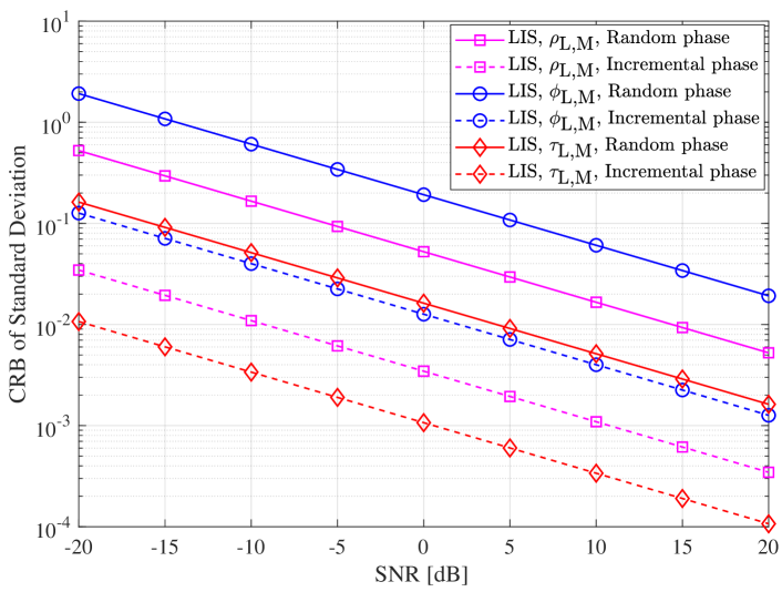
Figure 2: The impact of phases on CRB of standard deviation of channel parameters in the reflection path with $N_{\text{L}}=100$.

V-B Impact of the LIS: Number of Elements

In this experiment, we set $\omega_{i}=2\pi(i-1)\frac{d}{\lambda}[\sin(\theta_{\text{L,M}})-\sin(\phi_{\text{B,L}})]$ and SNR to 5 dB. The number of LIS elements plays a critical role on the estimation performance of channel parameters in the reflection path. The CRB of normalized standard deviation of $\tau_{\text{L,M}}$, $\phi_{\text{L,M}}$, and $\rho_{\text{L,M}}$ are inversely proportional to the number of elements in the LIS, e.g., $N_{\text{L}}$. As verified in Fig. 3, the larger the number of elements in the LIS, the better the estimation performance of the channel parameters. With around $100$ LIS elements, the estimation performance can be improved around $100$ times from the results shown in Fig. 3. In the legends, $\rho_{\text{B,S,M}}$, $\phi_{\text{B,S,M}}$, and $\tau_{\text{B,S,M}}$ denote the path loss, AoA, and ToA of the NLoS path via the scatter, respectively, for the benchmark scheme. Due to the fixed number of scatter, the estimation performance of the benchmark scheme stays unchanged. Note that the increase of elements does not have any great impact on the estimation accuracy of channel parameters of the direct path, which is not difficult to understand based on the FIM $\bar{{\mathbf{J}}}[n]$.

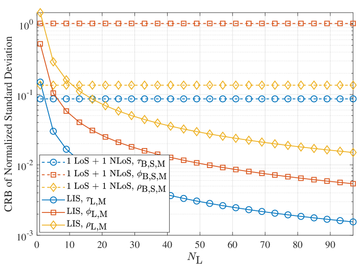
Figure 3: CRB of normalized standard deviation of channel parameters versus the number of LIS elements.

V-C PEB and OEB

In this subsection, we evaluate the impact of the number of LIS elements on both the PEB and the OEB while fixing $\omega_{i}=2\pi(i-1)\frac{d}{\lambda}[\sin(\theta_{\text{L,M}})-\sin(\phi_{\text{B,L}})]$. As shown in Figs. 4 and 5, the increase of elements improves the positioning performance. Even with the help of a $40$-element LIS, around 3 dB gain can be achieved when the OEB is at the level of $10^{-2}$. It should be noted that the performance enhancement mainly come from the improvement of the NLoS via the LIS.

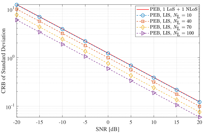
Figure 4: PEB versus the SNR.

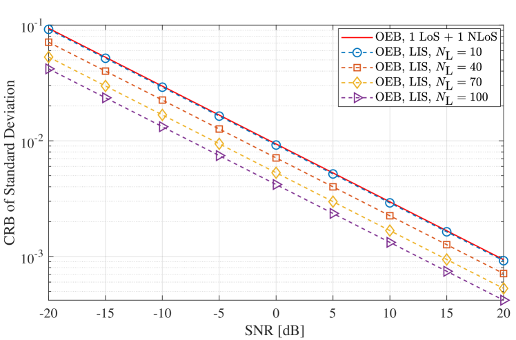
Figure 5: OEB versus the SNR.

VI Conclusions

We have studied the fundamental limits of mmWave MIMO positioning with the aid of a LIS. The impact of the number of LIS elements and the phases of LIS elements on the estimation of channel parameters has been investigated. This in turn, helps the analyses on the positioning and orientation error bounds. The comparison has been made between the positioning system with and without the assistance of LIS to show the potential benefits brought by the introduction of LIS even with passive elements. Since the beamformer design at BS and phase shifter design at LIS play a critical role in the positioning, the joint consideration of them will be left as our future investigation.

Appendix A Derivation of FIM

The derivation of the FIM on all the channel parameters is shown as follows:

$$\Psi_{n}(\tau_{\text{B,M}},\tau_{\text{B,M}})=\frac{PN_{\text{M}}\rho^{2}_{\text{B,M}}}{\sigma^{2}}\frac{(2\pi nB)^{2}}{N^{2}}\|\boldsymbol{\alpha}^{H}_{t}(\theta_{\text{B,M}}){\mathbf{F}}{\mathbf{x}}[n]\|_{2}^{2},$$ (18)

$$\Psi_{n}(\tau_{\text{B,M}},\theta_{\text{B,M}})=\frac{P\rho^{2}_{\text{B,M}}}{\sigma^{2}}\Re\{j2\pi\frac{nB}{N}({\mathbf{x}}[n])^{H}{\mathbf{F}}^{H}\boldsymbol{\alpha}_{t}(\theta_{\text{B,M}})\dot{\boldsymbol{\alpha}}^{H}_{t}(\theta_{\text{B,M}}){\mathbf{F}}{\mathbf{x}}[n]\},$$ (19)

$$\Psi_{n}(\tau_{\text{B,M}},\phi_{\text{B,M}})=\frac{P\rho^{2}_{\text{B,M}}}{\sigma^{2}}$$

$$\;\;\;\;\;\;\;\;\;\;\;\;\times\Re\{j2\pi\frac{nB}{N}({\mathbf{x}}[n])^{H}{\mathbf{F}}^{H}\boldsymbol{\alpha}_{t}(\theta_{\text{B,M}})\boldsymbol{\alpha}^{H}_{r}(\phi_{\text{B,M}})\dot{\boldsymbol{\alpha}}_{r}(\phi_{\text{B,M}})\boldsymbol{\alpha}^{H}_{t}(\theta_{\text{B,M}}){\mathbf{F}}{\mathbf{x}}[n]\},$$ (20)

$$\Psi_{n}(\tau_{\text{B,M}},\rho_{\text{B,M}})=\frac{P\rho_{\text{B,M}}}{\sigma^{2}}\|\boldsymbol{\alpha}^{H}_{t}(\theta_{\text{B,M}}){\mathbf{F}}{\mathbf{x}}[n]\|_{2}^{2}\Re\{j2\pi\frac{nB}{N}\}=0,$$ (21)

$$\Psi_{n}(\tau_{\text{B,M}},\tau_{\text{L,M}})=\frac{P\rho_{\text{B,M}}\rho_{\text{B,L}}\rho_{\text{L,M}}}{\sigma^{2}}\frac{(2\pi nB)^{2}}{N^{2}}$$

$$\;\;\;\;\;\;\;\;\;\;\;\;\times\Re\{\beta[n]\xi[n]({\mathbf{x}}[n])^{H}{\mathbf{F}}^{H}\boldsymbol{\alpha}_{t}(\theta_{\text{B,M}})\boldsymbol{\alpha}^{H}_{r}(\phi_{\text{B,M}})\boldsymbol{\alpha}_{r}(\phi_{\text{L,M}})\},$$ (22)

$$\Psi_{n}(\tau_{\text{B,M}},\phi_{\text{L,M}})=\frac{P\rho_{\text{B,M}}\rho_{\text{B,L}}\rho_{\text{L,M}}}{\sigma^{2}}$$

$$\;\;\;\;\;\;\;\;\;\;\;\;\times\Re\{j2\pi\frac{nB}{N}\beta[n]\xi[n]({\mathbf{x}}[n])^{H}{\mathbf{F}}^{H}\boldsymbol{\alpha}_{t}(\theta_{\text{B,M}})\boldsymbol{\alpha}^{H}_{r}(\phi_{\text{B,M}})\dot{\boldsymbol{\alpha}}_{r}(\phi_{\text{L,M}})\},$$ (23)

$$\Psi_{n}(\tau_{\text{B,M}},\rho_{\text{L,M}})=\frac{P\rho_{\text{B,M}}\rho_{\text{B,L}}}{\sigma^{2}}$$

$$\;\;\;\;\;\;\;\;\;\;\;\;\times\Re\{j2\pi\frac{nB}{N}\beta[n]\xi[n]({\mathbf{x}}[n])^{H}{\mathbf{F}}^{H}\boldsymbol{\alpha}_{t}(\theta_{\text{B,M}})\boldsymbol{\alpha}^{H}_{r}(\phi_{\text{B,M}})\boldsymbol{\alpha}_{r}(\phi_{\text{L,M}})\},$$ (24)

$$\Psi_{n}(\theta_{\text{B,M}},\theta_{\text{B,M}})=\frac{PN_{\text{M}}\rho^{2}_{\text{B,M}}}{\sigma^{2}}\|\dot{\boldsymbol{\alpha}}^{H}_{t}(\theta_{\text{B,M}}){\mathbf{F}}{\mathbf{x}}[n]\|_{2}^{2},$$ (25)

$$\Psi_{n}(\theta_{\text{B,M}},\phi_{\text{B,M}})=\frac{P\rho^{2}_{\text{B,M}}}{\sigma^{2}}$$

$$\;\;\;\;\;\;\;\;\;\;\;\;\times\Re\{({\mathbf{x}}[n])^{H}{\mathbf{F}}^{H}\dot{\boldsymbol{\alpha}}_{t}(\theta_{\text{B,M}})\boldsymbol{\alpha}^{H}_{r}(\phi_{\text{B,M}})\dot{\boldsymbol{\alpha}}_{r}(\phi_{\text{B,M}})\boldsymbol{\alpha}^{H}_{t}(\theta_{\text{B,M}}){\mathbf{F}}{\mathbf{x}}[n]\},$$ (26)

$$\Psi_{n}(\theta_{\text{B,M}},\rho_{\text{B,M}})=\frac{PN_{\text{M}}\rho_{\text{B,M}}}{\sigma^{2}}\Re\{({\mathbf{x}}[n])^{H}{\mathbf{F}}^{H}\dot{\boldsymbol{\alpha}}_{t}(\theta_{\text{B,M}})\boldsymbol{\alpha}^{H}_{t}(\theta_{\text{B,M}}){\mathbf{F}}{\mathbf{x}}[n]\},$$ (27)

$$\Psi_{n}(\theta_{\text{B,M}},\tau_{\text{L,M}})=\frac{P\rho_{\text{B,M}}\rho_{\text{B,L}}\rho_{\text{L,M}}}{\sigma^{2}}$$

$$\;\;\;\;\;\;\;\;\;\;\;\;\times\Re\{-j2\pi\frac{nB}{N}\beta[n]\xi[n]({\mathbf{x}}[n])^{H}{\mathbf{F}}^{H}\dot{\boldsymbol{\alpha}}_{t}(\theta_{\text{B,M}})\boldsymbol{\alpha}^{H}_{r}(\phi_{\text{B,M}})\boldsymbol{\alpha}_{r}(\phi_{\text{L,M}})\},$$ (28)

$$\Psi_{n}(\theta_{\text{B,M}},\phi_{\text{L,M}})=\frac{P\rho_{\text{B,M}}\rho_{\text{B,L}}\rho_{\text{L,M}}}{\sigma^{2}}$$

$$\;\;\;\;\;\;\;\;\;\;\;\;\times\Re\{\beta[n]\xi[n]({\mathbf{x}}[n])^{H}{\mathbf{F}}^{H}\dot{\boldsymbol{\alpha}}_{t}(\theta_{\text{B,M}})\boldsymbol{\alpha}^{H}_{r}(\phi_{\text{B,M}})\dot{\boldsymbol{\alpha}}_{r}(\phi_{\text{L,M}})\},$$ (29)

$$\Psi_{n}(\theta_{\text{B,M}},\rho_{\text{L,M}})=\frac{P\rho_{\text{B,M}}\rho_{\text{B,L}}}{\sigma^{2}}$$

$$\;\;\;\;\;\;\;\;\;\;\;\;\times\Re\{\beta[n]\xi[n]({\mathbf{x}}[n])^{H}{\mathbf{F}}^{H}\dot{\boldsymbol{\alpha}}_{t}(\theta_{\text{B,M}})\boldsymbol{\alpha}^{H}_{r}(\phi_{\text{B,M}})\boldsymbol{\alpha}_{r}(\phi_{\text{L,M}})\},$$ (30)

$$\Psi_{n}(\phi_{\text{B,M}},\phi_{\text{B,M}})=\frac{P\rho^{2}_{\text{B,M}}}{\sigma^{2}}\|\dot{\boldsymbol{\alpha}}_{r}(\phi_{\text{B,M}})\boldsymbol{\alpha}^{H}_{t}(\theta_{\text{B,M}}){\mathbf{F}}{\mathbf{x}}[n]\|_{2}^{2},$$ (31)

$$\Psi_{n}(\phi_{\text{B,M}},\rho_{\text{B,M}})=\frac{P\rho_{\text{B,M}}}{\sigma^{2}}$$

$$\;\;\;\;\;\;\;\;\;\;\;\;\times\Re\{({\mathbf{x}}[n])^{H}{\mathbf{F}}^{H}\boldsymbol{\alpha}_{t}(\theta_{\text{B,M}})\dot{\boldsymbol{\alpha}}^{H}_{r}(\phi_{\text{B,M}})\boldsymbol{\alpha}_{r}(\phi_{\text{B,M}})\boldsymbol{\alpha}^{H}_{t}(\theta_{\text{B,M}}){\mathbf{F}}{\mathbf{x}}[n]\},$$ (32)

$$\Psi_{n}(\phi_{\text{B,M}},\tau_{\text{L,M}})=\frac{P\rho_{\text{B,M}}\rho_{\text{B,L}}\rho_{\text{L,M}}}{\sigma^{2}}$$

$$\;\;\;\;\;\;\;\;\;\;\;\;\times\Re\{-j2\pi\frac{nB}{N}\beta[n]\xi[n]({\mathbf{x}}[n])^{H}{\mathbf{F}}^{H}\boldsymbol{\alpha}_{t}(\theta_{\text{B,M}})\dot{\boldsymbol{\alpha}}^{H}_{r}(\phi_{\text{B,M}})\boldsymbol{\alpha}_{r}(\phi_{\text{L,M}})\},$$ (33)

$$\Psi_{n}(\phi_{\text{B,M}},\phi_{\text{L,M}})=\frac{P\rho_{\text{B,M}}\rho_{\text{B,L}}\rho_{\text{L,M}}}{\sigma^{2}}$$

$$\;\;\;\;\;\;\;\;\;\;\;\;\times\Re\{\beta[n]\xi[n]({\mathbf{x}}[n])^{H}{\mathbf{F}}^{H}\boldsymbol{\alpha}_{t}(\theta_{\text{B,M}})\dot{\boldsymbol{\alpha}}^{H}_{r}(\phi_{\text{B,M}})\dot{\boldsymbol{\alpha}}_{r}(\phi_{\text{L,M}})\},$$ (34)

$$\Psi_{n}(\phi_{\text{B,M}},\rho_{\text{L,M}})=\frac{P\rho_{\text{B,M}}\rho_{\text{B,L}}}{\sigma^{2}}$$

$$\;\;\;\;\;\;\;\;\;\;\;\;\times\Re\{\beta[n]\xi[n]({\mathbf{x}}[n])^{H}{\mathbf{F}}^{H}\boldsymbol{\alpha}_{t}(\theta_{\text{B,M}})\dot{\boldsymbol{\alpha}}^{H}_{r}(\phi_{\text{B,M}})\boldsymbol{\alpha}_{r}(\phi_{\text{L,M}})\},$$ (35)

$$\Psi_{n}(\rho_{\text{B,M}},\rho_{\text{B,M}})=\frac{PN_{\text{M}}}{\sigma^{2}}\|\boldsymbol{\alpha}^{H}_{t}(\theta_{\text{B,M}}){\mathbf{F}}{\mathbf{x}}[n]\|_{2}^{2},$$ (36)

$$\Psi_{n}(\rho_{\text{B,M}},\tau_{\text{L,M}})=\frac{P\rho_{\text{B,L}}\rho_{\text{L,M}}}{\sigma^{2}}$$

$$\;\;\;\;\;\;\;\;\;\;\;\;\times\Re\{-j2\pi\frac{nB}{N}\beta[n]\xi[n]({\mathbf{x}}[n])^{H}{\mathbf{F}}^{H}\boldsymbol{\alpha}_{t}(\theta_{\text{B,M}})\boldsymbol{\alpha}^{H}_{r}(\phi_{\text{B,M}})\boldsymbol{\alpha}_{r}(\phi_{\text{L,M}})\},$$ (37)

$$\Psi_{n}(\rho_{\text{B,M}},\phi_{\text{L,M}})=\frac{P\rho_{\text{B,L}}\rho_{\text{L,M}}}{\sigma^{2}}$$

$$\;\;\;\;\;\;\;\;\;\;\;\;\times\Re\{\beta[n]\xi[n]({\mathbf{x}}[n])^{H}{\mathbf{F}}^{H}\boldsymbol{\alpha}_{t}(\theta_{\text{B,M}})\boldsymbol{\alpha}^{H}_{r}(\phi_{\text{B,M}})\dot{\boldsymbol{\alpha}}_{r}(\phi_{\text{L,M}})\},$$ (38)

$$\Psi_{n}(\rho_{\text{B,M}},\rho_{\text{L,M}})=\frac{P\rho_{\text{B,L}}}{\sigma^{2}}$$

$$\;\;\;\;\;\;\;\;\;\;\;\;\times\Re\{\beta[n]\xi[n]({\mathbf{x}}[n])^{H}{\mathbf{F}}^{H}\boldsymbol{\alpha}_{t}(\theta_{\text{B,M}})\boldsymbol{\alpha}^{H}_{r}(\phi_{\text{B,M}})\boldsymbol{\alpha}_{r}(\phi_{\text{L,M}})\},$$ (39)

$$\Psi_{n}(\tau_{\text{L,M}},\tau_{\text{L,M}})=\frac{PN_{\text{M}}\rho^{2}_{\text{B,L}}\rho^{2}_{\text{L,M}}}{\sigma^{2}}\frac{(2\pi nB)^{2}|\beta[n]|^{2}}{N^{2}},$$ (40)

$$\Psi_{n}(\tau_{\text{L,M}},\phi_{\text{L,M}})=\frac{P\rho^{2}_{\text{B,L}}\rho^{2}_{\text{L,M}}}{\sigma^{2}}$$

$$\;\;\;\;\;\;\;\;\;\;\;\;\times\Re\{j2\pi\frac{nB}{N}(\beta[n])^{*}\boldsymbol{\alpha}^{H}_{r}(\phi_{\text{L,M}})\dot{\boldsymbol{\alpha}}_{r}(\phi_{\text{L,M}})\boldsymbol{\Omega}\boldsymbol{\alpha}_{r}(\phi_{\text{B,L}})\boldsymbol{\alpha}^{H}_{t}(\theta_{\text{B,L}}){\mathbf{F}}{\mathbf{x}}[n]\},$$ (41)

$$\Psi_{n}(\tau_{\text{L,M}},\rho_{\text{L,M}})=\frac{P\rho^{2}_{\text{B,L}}\rho_{\text{L,M}}|\beta[n]|^{2}}{\sigma^{2}}\Re\{j2\pi\frac{nB}{N}\}=0,$$ (42)

$$\Psi_{n}(\phi_{\text{L,M}},\phi_{\text{L,M}})=\frac{P\rho^{2}_{\text{B,L}}\rho^{2}_{\text{L,M}}}{\sigma^{2}}\|\beta[n]\dot{\boldsymbol{\alpha}}_{r}(\phi_{\text{L,M}})\|_{2}^{2},$$ (43)

$$\Psi_{n}(\phi_{\text{L,M}},\rho_{\text{L,M}})=\frac{P\rho^{2}_{\text{B,L}}\rho_{\text{L,M}}}{\sigma^{2}}$$

$$\;\;\;\;\;\;\;\;\;\;\;\;\times\Re\{(\beta[n])^{*}\boldsymbol{\alpha}^{H}_{r}(\phi_{\text{L,M}})\dot{\boldsymbol{\alpha}}_{r}(\phi_{\text{L,M}})\boldsymbol{\Omega}\boldsymbol{\alpha}_{r}(\phi_{\text{B,L}})\boldsymbol{\alpha}^{H}_{t}(\theta_{\text{B,L}}){\mathbf{F}}{\mathbf{x}}[n]\},$$ (44)

$$\Psi_{n}(\rho_{\text{L,M}},\rho_{\text{L,M}})=\frac{PN_{\text{M}}\rho^{2}_{\text{B,L}}|\beta[n]|^{2}}{\sigma^{2}},$$ (45)

where $\dot{\boldsymbol{\alpha}}_{t}(\theta_{\text{B,M}})=\partial\boldsymbol{\alpha}_{t}(\theta_{\text{B,M}})/\partial\theta_{\text{B,M}}={\mathbf{D}}_{t}(\theta_{\text{B,M}})\alpha_{t}(\theta_{\text{B,M}})$, $\dot{\boldsymbol{\alpha}}_{r}(\phi_{\text{B,M}})=\partial\boldsymbol{\alpha}_{r}(\phi_{\text{B,M}})/\partial\phi_{\text{B,M}}={\mathbf{D}}_{r}(\phi_{\text{B,M}})\alpha_{r}(\phi_{\text{B,M}})$, $\dot{\boldsymbol{\alpha}}_{r}(\phi_{\text{L,M}})=\partial\boldsymbol{\alpha}_{r}(\phi_{\text{L,M}})/\partial\phi_{\text{L,M}}={\mathbf{D}}_{r}(\phi_{\text{L,M}})\alpha_{r}(\phi_{\text{L,M}})$ with ${\mathbf{D}}_{t}(\theta_{\text{B,M}})=j2\pi\frac{d}{\lambda}\cos(\theta_{\text{B,M}})\mathrm{diag}(0,1,\cdots,i,\cdots,N_{\text{B}}-1)$, ${\mathbf{D}}_{r}(\phi_{\text{B,M}})=j2\pi\frac{d}{\lambda}\cos(\phi_{\text{B,M}})\mathrm{diag}(0,1,\cdots,i,\cdots,N_{\text{M}}-1)$, ${\mathbf{D}}_{r}(\phi_{\text{L,M}})=j2\pi\frac{d}{\lambda}\cos(\phi_{\text{L,M}})\mathrm{diag}(0,1,\cdots,i,\cdots,N_{\text{M}}-1)$, $\xi[n]=e^{-j[2\pi(\tau_{\text{B,L}}+\tau_{\text{L,M}}-\tau_{\text{B,M}})\frac{nB}{N}]}$, and $\beta[n]=\boldsymbol{\alpha}^{H}_{t}(\theta_{\text{L,M}})\boldsymbol{\Omega}\boldsymbol{\alpha}_{r}(\phi_{\text{B,L}})\boldsymbol{\alpha}^{H}_{t}(\theta_{\text{B,L}}){\mathbf{F}}{\mathbf{x}}[n]$.

References

- [1] A. Yassin, Y. Nasser, M. Awad, A. Al-Dubai, R. Liu, C. Yuen, R. Raulefs, and E. Aboutanios, “Recent advances in indoor localization: A survey on theoretical approaches and applications,” IEEE Commun. Surveys Tuts., vol. 19, no. 2, pp. 1327–1346, Secondquarter 2017.
- [2] V. Savic and E. G. Larsson, “Fingerprinting-based positioning in distributed massive MIMO systems,” in IEEE Vehicular Technology Conference (VTC2015-Fall), Sep. 2015, pp. 1–5.
- [3] X. Wang, L. Gao, S. Mao, and S. Pandey, “CSI-based fingerprinting for indoor localization: A deep learning approach,” IEEE Trans. Veh. Technol., vol. 66, no. 1, pp. 763–776, Jan 2017.
- [4] A. Shahmansoori, G. E. Garcia, G. Destino, G. Seco-Granados, and H. Wymeersch, “Position and orientation estimation through millimeter-wave mimo in 5G systems,” IEEE Trans. Wireless Commun., vol. 17, no. 3, pp. 1822–1835, Mar. 2018.
- [5] Z. Abu-Shaban, X. Zhou, T. Abhayapala, G. Seco-Granados, and H. Wymeersch, “Error bounds for uplink and downlink 3D localization in 5G millimeter wave systems,” IEEE Trans. Wireless Commun., vol. 17, no. 8, pp. 4939–4954, Aug 2018.
- [6] H. Zhao, L. Zhang, and Y. Shen, “On the optimal beamspace design for direct localization systems,” in proc. of IEEE International Conference on Communications (ICC), May 2018, pp. 1–6.
- [7] R. Koirala, B. Denis, B. Uguen, D. Dardari, and H. Wymeersch, “Localization optimal multi-user beamforming with multi-carrier mmwave MIMO,” in proc. of IEEE International Symposium on Personal, Indoor and Mobile Radio Communications (PIMRC), Sep. 2018, pp. 1–7.
- [8] A. Kakkavas, G. Seco-Granados, H. Wymeersch, M. H. C. García, R. A. Stirling-Gallacher, and J. A. Nossek, “5G downlink multi-beam signal design for LOS positioning,” in IEEE Globecom, Dec. 2019, pp. 1–6.
- [9] C. Huang, A. Zappone, G. C. Alexandropoulos, M. Debbah, and C. Yuen, “Large intelligent surfaces for energy efficiency in wireless communication,” CoRR, vol. abs/1810.06934, 2018. [Online]. Available: http://arxiv.org/abs/1810.06934
- [10] E. Basar, M. Di Renzo, J. de Rosny, M. Debbah, M.-S. Alouini, and R. Zhang, “Wireless Communications Through Reconfigurable Intelligent Surfaces,” arXiv e-prints, p. arXiv:1906.09490, Jun 2019.
- [11] S. Hu, F. Rusek, and O. Edfors, “Beyond massive MIMO: The potential of positioning with large intelligent surfaces,” IEEE Trans. Signal Process., vol. 66, no. 7, pp. 1761–1774, Apr 2018.
- [12] D. L. Donoho, “Compressed sensing,” IEEE Trans. Inf. Theory, vol. 52, no. 4, pp. 1289–1306, Apr 2006.
- [13] G. Hannak, A. Perelli, N. Goertz, G. Matz, and M. E. Davies, “Performance analysis of approximate message passing for distributed compressed sensing,” IEEE J. Sel. Topics Signal Process., vol. 12, no. 5, pp. 857–870, Oct 2018.
- [14] T. S. Rappaport, S. Sun, R. Mayzus, H. Zhao, Y. Azar, K. Wang, G. N. Wong, J. K. Schulz, M. Samimi, and F. Gutierrez, “Millimeter wave mobile communications for 5G cellular: It will work!” IEEE Access, vol. 1, pp. 335–349, 2013.