GraphRQI: Classifying Driver Behaviors Using Graph Spectrums

Abstract

We present a novel algorithm (GraphRQI) to identify driver behaviors from road-agent trajectories. Our approach assumes that the road-agents exhibit a range of driving traits, such as aggressive or conservative driving. Moreover, these traits affect the trajectories of nearby road-agents as well as the interactions between road-agents. We represent these inter-agent interactions using unweighted and undirected traffic graphs. Our algorithm classifies the driver behavior using a supervised learning algorithm by reducing the computation to the spectral analysis of the traffic graph. Moreover, we present a novel eigenvalue algorithm to compute the spectrum efficiently. We provide theoretical guarantees for the running time complexity of our eigenvalue algorithm and show that it is faster than previous methods by 2 times. We evaluate the classification accuracy of our approach on traffic videos and autonomous driving datasets corresponding to urban traffic. In practice, GraphRQI achieves an accuracy improvement of up to $25\%$ over prior driver behavior classification algorithms. We also use our classification algorithm to predict the future trajectories of road-agents.

I Introduction

Autonomous driving is an active area of research [1, 2] and includes many issues related to perception, navigation, and control [2]. While some of the earlier work was focused on autonomous driving in mostly empty roads or highways, there is considerable recent work on developing technologies in urban scenarios. These urban scenarios consist of a variety of road-agents corresponding to vehicles, buses, trucks, bicycles, and pedestrians. In order to perform collision-free navigation, it is important to track the location of these road-agents [3, 4] and predict their trajectory in the near future [5, 6, 7, 8, 9, 10, 11]. These tasks can be improved with a better understanding and prediction of driver behavior and performing behavior-aware planning [12, 13, 6, 14]. For example, drivers can navigate dangerous traffic situations by identifying the aggressive drivers and avoiding them or keeping a distance. At the same time, there is a clear distinction between such driver behaviors and maneuver-based road-agent behaviors [15, 16, 17, 18]. According to studies in traffic psychology [19, 20, 21], driver behavior corresponds to labels for various driving traits, such as aggressive and conservative driving [19, 20, 21]. These studies further show that traffic flow and road-agent trajectories are significantly affected by driver behaviors. For instance, an aggressive road-agent overtaking a vehicle may cause the vehicle to slow down, or an overly cautious driver may drive slowly and cause congestion.

Our goal is to classify the drivers according to their behaviors in a given traffic video. The two most widely used behavior labels used to classify drivers are aggressive and conservative [22, 23, 24]. Recent studies have also explored more granular behaviors, such as reckless, impatient, careful and timid [25, 26]. For instance, impatient drivers show different traits (e.g., over-speeding, overtaking) than reckless drivers (e.g., driving in the opposite direction to the traffic) [25], but both can be regarded as aggressive. Similarly, timid drivers may drive slower than the speed limit [26], while careful drivers obey the traffic rules. However, both of them are marked as conservative drivers. In this paper, we consider a total of six different classes of driver behavior — impatient, reckless, threatening, careful, cautious, and timid [12]. For the rest of the paper, we collectively refer to the first three as aggressive driving, while the last three are categorized as part of conservative driving.

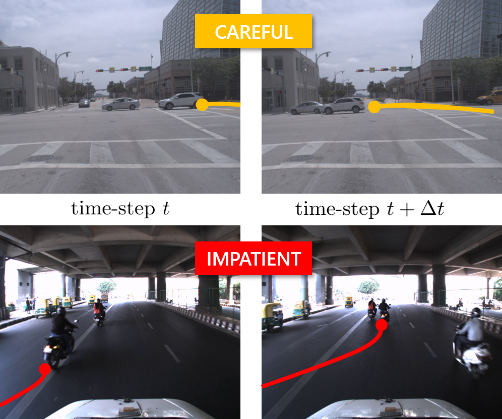
Figure 1: GraphRQI predicts the behaviors of road-agents in dense and heterogeneous traffic from one of the following classes–impatient, reckless, threatening, careful, cautious, timid. Our approach is up to 25% more accurate than prior behavior prediction methods.

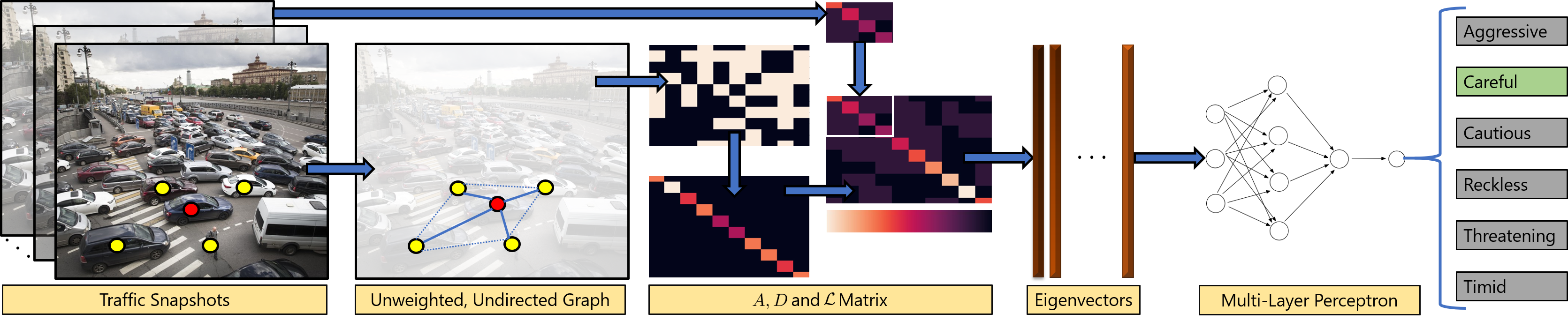
Figure 2: Overview of GraphRQI: At any instance of traffic, we use the current trajectories to form an unweighted and undirected graphical representation. We can then compute the adjacency matrix, the degree matrix, and the Laplacian matrix of the graph. Note that the principal leading submatrix of the Laplacian can be obtained from the Laplacian of the traffic from previous time-steps. We use our eigenvalue algorithm to compute the spectrum of the Laplacian, which is then used for training via a multi-layer perceptron to predict the driver behavior.

Since the behavior of individual drivers directly influences the trajectories of all other drivers in their neighborhood, we can represent the drivers as the nodes of a sparse, undirected, and unweighted graph, and the interactions between the drivers through edges between the corresponding nodes. In our formulation, we analyze the spectral properties of such a graph for behavior classification. However, there are a few challenges in calculating the spectrum of such graphs. First, traffic flow is dynamic, therefore the number of edges in the graph changes at each time-step. Second, the number of nodes in the graph tends to increase monotonically with each time-step, since retaining information on past interactions is useful for predicting current and future behaviors of other drivers [7]. This is a problem for current state-of-the-art methods that perform graph spectral analysis  [27], as the computational complexity grows at least as $\mathcal{O}(n^{1.5})$, where $n$ is the number of nodes in the graph. In order to classify the behaviors, we need to design efficient methods to perform spectral analysis of such traffic graphs.

Main Results: We present a novel algorithm to classify driver behaviors from road-agent trajectories. Our approach is general, and we don’t make any assumption about traffic density, heterogeneity, or the underlying scenarios. The trajectories are extracted from traffic videos or other sensor data, and the resulting behaviors are classified among the three aggressive or three conservative behaviors described above. In order to efficiently classify the behavior, we present two novel algorithms:

1. A classification algorithm, GraphRQI, that takes as input road-agent trajectories, converts them into a dynamic-graph-based representation of the traffic, and predicts driver behaviors as one of six labels from the spectrum of the dynamic graph.

2. An eigenvalue algorithm that updates the spectrum of the dynamic traffic graph with $n$ current nodes in $\mathcal{O}(n)$ time, up from $\mathcal{O}(n^{1.5})$ required by prior methods.

Finally, we demonstrate an application where knowledge of the behavior of a road-agent allows nearby road-agents to generate efficient and safer paths based on different behavioral characteristics. We have compared our algorithm with prior classification schemes and observe the following benefits:

• Accuracy improvement: We report improvement of up to $20\%$ and $25\%$ in the weighted classification accuracy on the TRAF dataset [9] and the Argoverse dataset [28], respectively.

• Speed improvement: With up to $100$ drivers, the runtime of our eigenvalue algorithm is $10$ milliseconds which is a speed of up to $2.348$ seconds over prior works for calculating the spectrums of dynamic traffic graph.

II Related Work

II-A Driver Behavior and Intent Prediction

There is a large body of research on driver behavior and intent prediction. Furthermore, many studies have been performed that provides insights into factors that contribute to different driver behavior. Feng et al. [29] proposed five driver characteristics (age, gender, personality via blood test, and education level) and four environmental factors (weather, traffic situation, quality of road infrastructure, and other cars’ behavior), and mapped them to 3 levels of aggressiveness (driving safely, verbally abusing other drivers, and taking action against other drivers). Rong et al. [22] presented a similar study but instead used different features such as blood pressure, hearing, and driving experience to conclude that aggressive drivers tailgate and weave in and out of traffic. Dahlen et al. [24] studied the relationships between driver personality and aggressive driving using the five-factor-model [30]. Aljaafreh et al. [31] categorized driving behaviors into four classes: Below normal, Normal, Aggressive, and Very aggressive, in accordance with accelerometer data. Social Psychology studies [32, 33] have examined the aggressiveness according to the background of the driver, including age, gender, violation records, power of cars, occupation, etc. Mouloua et al. [34] designed a questionnaire on subjects’ previous aggressive driving behavior and concluded that these drivers also repeated those behaviors under a simulated environment. However, the driver features used by these methods cannot be computed easily for autonomous driving in new and unknown environments, which mainly rely on visual sensors.

Several methods have analyzed driver behavior using visual and other information. Murphey et al. [35] conducted an analysis on the aggressiveness of drivers and observed that longitudinal (changing lanes) jerk is more related to aggressiveness than progressive (along the lane) jerk (i.e., rate of change in acceleration). Mohamad et al. [36] detected abnormal driving styles using speed, acceleration, and steering wheel movement, which indicated the direction of vehicles. Qi et al. [37] studied driving styles with respect to speed and acceleration. Shi et al. [38] pointed out that deceleration is not very indicative of the aggressiveness of drivers, but measurements of throttle opening, which are associated with acceleration, were more helpful in identifying aggressive drivers. Wang et al. [39] classified drivers into two categories, aggressive and normal, using speed and throttle opening captured by a simulator. Sadigh et al. [40] proposed a data-driven model based on Convex Markov Chains to predict whether a driver is paying attention while driving. Some recent approaches also utilize RL (reinforcement learning) and imitation learning techniques to teach networks to recognize various driver intentions [41, 42], while others have applied RNN and LSTM-based networks to perform data-driven driver intent prediction [43, 44]. Apart from behavior prediction, some methods have been proposed for behavior modeling [45, 46, 47, 48, 49]. In our case, we exploit the spectrum of dynamic traffic graphs to predict driver behaviors, which is complementary to these approaches and can be combined with such methods.

II-B Supervised Learning Using Graphs

Bruna et al. [50] introduce supervised learning using convolutions on graphs via graph convolutional networks (GCNs). Kipf et al. [51] extend GCNs to self-supervised learning. However, these methods are restricted to static graphs. In order to model the temporal nature of traffic using graphs, Yu et al. [52] used a Spatio-temporal GCN (STGCN). The authors use recurrent neural networks to compute the temporal features of the dynamic traffic network. TIMERS [53] incrementally computes the spectrum using incremental Singular Value Decomposition (SVD) [54]. The method implemented a restart on the SVD when the error increases above a threshold. Li et al. [55] proposed an algorithm for computing the spectrum for node classification tasks that support addition and deletions of edges.

III Background

Table I: Notations used in the paper.

Symbol	Description
$n$	Number of vehicles
$[m]$	{1,2,…,m}
$\lvert\cdot\rvert$	Number of non-zero elements in a vector or matrix.
$\mathcal{I}_{d}$	Set of indices corresponding to non-zero entries in a vector $d$.
$A_{\mathcal{S}}$	Set of columns of $A$, indexed by elements of $\mathcal{S}$.
$\mathcal{L}_{t}$	The $t^{\textrm{th}}$ Laplacian matrix in a sequence of sub-degree matrices.
$d=\textrm{dim}\mathcal{L}_{t}$	The dimension number of rows (or columns)) of the laplacian matrix .
$\delta$	A binary vector of length $n$ such that $\lvert\delta\rvert\ll n$
$U$	Eigenvector matrix
$\Lambda$	Diagonal matrix with eigenvalues on the diagonal.

Table II: Analytical Comparison of GraphRQI with classical and state-of-the-art eigenvector algorithms. In practice, our observed runtime is $10$ milliseconds which is a speed of up to $2.348$ seconds over prior works for calculating the spectrums of dynamic traffic graph.

Metric	SVD	IncrementalSVD [54]	RestartSVD [53]	TruncatedSVD	CG [27]	GraphRQI
Time	$\mathcal{O}(d^{3})$	$\mathcal{O}(\lvert\mathcal{L}_{t}\rvert r)$	$\mathcal{O}\Big{(}\lvert f(\mathcal{L}_{t})\rvert+\lvert g(\mathcal{L}_{t})\rvert k+\lvert g(\mathcal{L}_{t})_{\overline{\emptyset}}\rvert k^{2}\Big{)}$	$\mathcal{O}(dk^{2})$	$\mathcal{O}(d\sqrt{\kappa})$	$\mathcal{O}(\lvert\mathcal{L}^{\scriptscriptstyle-1}_{t}\rvert k)$
Space	$\mathcal{O}(d^{2})$	$\mathcal{O}(2\ dr)$	-	$\mathcal{O}(dk)$	$\mathcal{O}(d)$	$\mathcal{O}(d)$

Our overall objective is to classify all drivers in a traffic video into one of six behavior classes — impatient, reckless, threatening, careful, cautious, and timid. We assume that the trajectories of all the road-agents in the video are provided to us as the input. Given this input, we first construct a traffic graph at each time-step, with the number of road-agents during that time-step being the number of nodes and undirected, unweighted edges connecting the neighboring road-agents during that time-step. Next, we show that the spectrum of the Laplacian matrix of the graphs contains pertinent information to classify the nodes (drivers) into corresponding behavior classes (Section IV).

In this section, we give an overview of a graph spectrum and a brief overview of graph topology. Notations used frequently throughout the paper are presented in Table I.

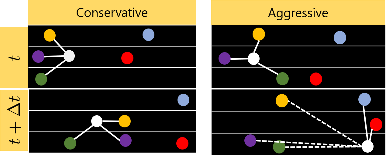
Figure 3: (left) Conservative vehicles tend to adhere to a uniform speed. Consequently, they form a uniform neighborhood that results in smooth topology in the traffic graph with short edges. (right) Aggressive drivers tend to display maneuvers such as tailgating, over-speeding, overtaking, and weaving. These maneuvers cause the road-agent to form sharper subgraphs in the traffic graph with long edges.

III-A Graph Spectrum

Given a graph $\mathcal{G}$, with a set of vertices $\mathcal{V}=\{v_{1},v_{2},\dots,v_{n}\}$ and a set of undirected, weighted edges $e_{ij}=e_{ji}=(v_{i},v_{j})$, $\mathcal{E}$, we define the entries of its adjacency matrix $A\in\mathbb{R}^{n\times n}$ as $A(i,j)=A(j,i)=e^{-d(v_{i},v_{j})}$ if $e_{ij}\in\mathcal{E}$ and $A(i,j)=0$, otherwise. The function $f(v_{i},v_{j})=e^{-d(v_{i},v_{j})}$ [56] denotes the interactions between any two road-agents, $v_{i}$ and $v_{j}$. The corresponding degree matrix $D\in\mathbb{R}^{n\times n}$ of the graph is a diagonal matrix with entries $D(i,i)=\sum_{j=1}^{n}A(i,j)$. The Laplacian matrix $\mathcal{L}=D-A$ of the graph has the entries,

$$\mathcal{L}(i,j)=\mathcal{L}(j,i)=\begin{cases}D(i,i)&\text{if $i=j$},\\ -e^{-d(v_{i},v_{j})}&\text{if $d(v_{i},v_{j})<\mu$},\\ 0&\text{otherwise.}\par\end{cases}$$

The matrix $U:=\{u_{i}|i=1\dots n\}$ of eigenvectors of $\mathcal{L}$ is called the spectrum of $\mathcal{L}$. It can be computed based on eigenvalue of $\mathcal{L}$.

III-B Graph Topology

The topology of a vertex $v_{i}$ in a graph refers to the arrangement of the adjacent neighborhood $\mathcal{N}_{i}$ of the vertex. For example, if $(v_{i},v_{j})\in\mathcal{E}$ $\forall v_{j}\in\mathcal{N}_{i}$ and $(v_{j},v_{k})\notin\mathcal{E}$ $\forall\{v_{j},v_{k}\}\in\mathcal{N}_{i}$, then we have a star topology [57]. The spectrum $U$ of the Laplacian matrix $\mathcal{L}$ can be used to compute the topology of a vertex. Let $w_{i}\in\mathbb{R}^{n}$ denote the $i^{\textrm{th}}$ column of the matrix $\mathcal{L}U$. Then the $j^{\textrm{th}}$ entry of $w_{i}$ is given by,

$$w_{i}(j)=D(j,j)u_{i}(j)-\sum u_{i}(k)=\sum\left(u_{i}(j)-u_{i}(k)\right).$$ (1)

Thus, the $j^{\textrm{th}}$ entry of $w_{i}$ equals the sum of edge values of all edges with $v_{j}$ as the common node. Since the arrangement of vertices depend on the edge lengths between them, this determines the topology of the graph.

IV Behavior Classification Using GraphRQI

In this section, we first show the construction of traffic graphs. Next, we present our eigenvalue algorithm. Finally, we present an analysis of our eigenvalue algorithm.

IV-A Computation of Traffic Graphs

Traffic-graphs and their topologies form the basis for our driver behavior classification approach. Behavioral traffic psychology studies show that aggressive drivers tend to display maneuvers such as tailgating, over-speeding, overtaking, and weaving [22]. From a topological perspective, all four maneuvers are similar (Figure 3, right) with a sharper graph structure with larger edge lengths. On the other hand, conservative vehicles tend to adhere to a uniform speed, forming a smoother topology with smaller edge lengths (Figure 3, left). Thus, topologies for aggressive behavior are different from the topologies for conservative behavior. We describe the formation of traffic-graphs next.

Algorithm 1 Our eigenvalue algorithm computes the $k$ eigenvectors, $\{u_{1},u_{2},\ldots,u_{k}\}$ of a Laplacian, $\mathcal{L}_{i}$.

1:$\mathcal{L}_{0},\Lambda_{0}$

2:for $j$ in range$(k)$ do

3:     Initialize $x_{\textrm{old}}$

4:     $x_{\textrm{new}}=x_{\textrm{old}}/\lVert x_{\textrm{old}}\rVert$

5:     while $\lVert x_{\textrm{new}}-x_{\textrm{old}}\rVert\leq\epsilon$ do

6:         $x_{\textrm{old}}=x_{\textrm{new}}/\lVert x_{\textrm{new}}\rVert$

7:         $x_{\textrm{new}}\leftarrow\textsc{update}(\sigma\sigma^{\top},\mathcal{L}_{t-1},\mu_{j})$      

8:     $u_{j}=x_{\textrm{new}}/\lVert x_{\textrm{new}}\rVert$ return $U=[u_{1},u_{2},\ldots,u_{k}]$

At the $t$-th time-step, we obtain the $k$-nearest neighbors [58] of each road-agent using their current trajectories. In our experiments, we heuristically choose $k=4$. We initialize an adjacency matrix $A_{t}$ with all zeros, and assign $A(i,j)=1$ if road-agents $v_{i},v_{j}$ are neighbors. We then form the Laplacian matrix (ala Section III-A) at the $t^{\textrm{th}}$ time-step, $\mathcal{L}_{t}=D_{t}-A_{t}$. As road-agents observe new neighbors, we update the Laplacian matrix using the following update:

$$\mathcal{L}_{t}=\left[\begin{array}[]{c|c}\mathcal{L}_{t-1}\rule[-5.59721pt]{0.0pt}{0.0pt}&0\rule[-5.59721pt]{0.0pt}{0.0pt}\\ \hline\cr 0\rule{0.0pt}{11.19443pt}&1\end{array}\right]+\delta\delta^{\top},$$

where $\mathcal{L}_{t-1}$ is the leading principal sub-matrix of $\mathcal{L}_{t}$ of order $k$ and $\delta$ is defined in Table I. For our experiments, we reset the Laplacian matrix after $T=100$ to avoid buffer overflow.

IV-B Eigenvalue Algorithm

Our eigenvalue algorithm is built upon the classical RQI algorithm [59] that computes an eigenvector $u$ that corresponds to an approximation of a given eigenvalue $\mu$ of a given matrix. However, the dominant step of the RQI consists of matrix inversion that generally requires $\mathcal{O}(d^{3})$ operations, and so the applicability of RQI to a sequence of dynamic ( or time-varying) matrices largely depends on two factors — computational complexity of matrix inversion, and the length of the sequence. For a sequence of dynamic Laplacian matrices, $\{\mathcal{L}_{1},\mathcal{L}_{2},\ldots,\mathcal{L}_{T}\}$, the main advantage of the GraphRQI approach is to be able to compute the eigenvector matrix, $U$, very efficiently by combining the following optimizations:

• Recursively exploit sub-$k$ matrix information.

• Exploit the sparsity and symmetry of Laplacian matrices to compute inverse Laplacian matrices efficiently.

We give the pseudo-code of our eigenvalue algorithm in Algorithm 1. At each time-step $t$, we compute $k$ eigenvectors of $\mathcal{L}_{t}$. For each eigenvector, we perform an iterative process. We begin by initializing a random vector. Next, we iteratively perform the following update rule until it converges to an eigenvector. For the $j^{\textrm{th}}$ eigenvector, the update rule is given as:

where sm refers to the Sherman-Morrison formula [60] that computes the inverse of a sum of a matrix and an outer product, $xx^{\top}$, where $x\in\mathbb{R}^{d\times 1}$ is a sparse vector, $\mu_{j}$ is the approximate eigenvalue corresponding to which we compute an eigenvector, $u_{j}$. $\mathcal{L}_{t-1},U_{t-1}$, and $\Lambda_{t-1}$ are the Laplacian, spectrum, and corresponding diagonal eigenvalue matrix of the previous time-step. $\delta$ is a sparse $\mathbb{R}^{d}$ vector where, if the $k^{\textrm{th}}$ entry of $\delta$ is denoted by $\delta(k)$, then the $k^{\textrm{th}}$ road-agent observes a new neighbor if $\delta(k)=1$.

Table III: Ablation study on TRAF and ARGO datasets. We perform a running time analysis of several eigenvalue algorithms. All experiments were performed on an 8 Core Intel Xeon(R) W2123 CPU clocked at 3.60GHz with 32 GB RAM to compute the eigenvectors for a $d\times d$ matrix, where $d$ is the number of road-agents. We also compare the accuracy of different supervised learning machine learning models and report the weighted classification accuracy.

	Eigenvalue Algorithms (Runtime)						GraphRQI + ML model (Accuracy)
Dataset	SVD	IncrementalSVD [54]	RestartSVD [53]	TruncatedSVD	CG	GraphRQI	LogReg	SVM	LSTM	GraphRQI
TRAF	34.2ms	67ms	1,644ms	37ms	2,365ms	16.9ms	69.1%	74.2%	71.4%	78.3%
ARGO	16.9ms	45ms	1,091ms	35ms	2,328ms	10ms	69.9%	75.0%	70.8%	89.9%

IV-C Graph Spectrum Analysis

We compute the spectrum of the graph that describes the topologies of traffic at various time-step to classify aggressive and conservative behaviors.

In Table II, we compare the time and space complexities of several state-of-the-art eigenvalue algorithms. For each of these methods, the input is a Laplacian matrix. We now state the theoretical guarantees for the running time and storage cost of our eigenvalue algorithm in the following theorems. All proofs are provided in the supplementary material.

Theorem IV.1.

Given a sequence, $\{\mathcal{L}_{1},\mathcal{L}_{2},\ldots,\mathcal{L}_{T}\}$, our eigenvalue algorithm for $\mathcal{L}_{t}$ converges cubically with a running time complexity of $\mathcal{O}(\lvert\mathcal{L}^{\scriptscriptstyle-1}_{t}\rvert k)$ for each Laplacian at time-step $t$, where $k\ll\textnormal{dim}(\mathcal{L}_{t})$, with a storage cost of $\mathcal{O}(d)$.

Informally, Theorem Lemma states that for a Laplacian matrix $\mathcal{L}_{t}$, the compuatation for each eigenvector requires $\mathcal{O}(\lvert\mathcal{L}^{\scriptscriptstyle-1}_{t}\rvert)$ operations, which is fewer than quadratic runtime algorithms that require $\mathcal{O}(d^{2})$ operations, since $\mathcal{O}(\lvert\mathcal{L}^{\scriptscriptstyle-1}_{t}\rvert)\ll d^{2}$. For a random intial iterate, $x$, our eigenvalue algorithm converges cubically, that is, at each iteration, $\lvert x_{\textrm{new}}-x_{\textrm{old}}\rvert=\mathcal{O}(\epsilon^{3})$.

Note that some eigenvalue algorithms make several assumptions in terms of running time complexity analysis. For example, the conjugate gradient method [27] requires $\mathcal{O}(d\sqrt{\kappa})$ operations. The success of conjugate gradient assumes the matrix is either well-conditioned or pre-conditioned by a preconditioning matrix, for which the running time becomes $\mathcal{O}(d^{1.5})$. IncrementalSVD [54] requires the matrix to be low-rank. In the general case, IncrementalSVD requires $\mathcal{O}(\lvert\mathcal{L}_{t}\rvert d)$ which becomes $\mathcal{O}(\lvert\mathcal{L}_{t}\rvert r)$ for low rank matrices with rank $r$. Our eigenvalue algorithm makes no such assumptions. We now state a lemma, related to our Laplacian matrix, that is used to prove Theorem Lemma.

Lemma IV.2.

The complexity of computing the inverse of a Laplacian at time-step $t$, $\mathcal{L}^{\scriptscriptstyle-1}_{t}$, grows as $\mathcal{O}(\lvert\mathcal{L}^{\scriptscriptstyle-1}_{t}\rvert)$.

The current best-case running-time complexity for inverting a $d\times d)$ matrix is $\mathcal{O}(d^{2.373})$ using a variation of the Coppersmith–Winograd algorithm [61]. We show that we can achieve an even lower runtime complexity for inverting our matrix in $\mathcal{O}(\lvert\mathcal{L}^{\scriptscriptstyle-1}_{t}\rvert)$, where $\mathcal{O}(\lvert\mathcal{L}^{\scriptscriptstyle-1}_{t}\rvert)\ll d^{2}$.

IV-D Behavior Classification

The graphs are constructed from the road-agent trajectories as described in Section IV-A. We then pass the spectrum of the traffic graphs as inputs to train a Multi-Layer Perceptron(MLP) [62] for behavior classification. The MLP is parametrized by a weight vector, $w$. Our goal is to learn the optimal parameters that minimize the squared error loss,

$$f(w)=\frac{1}{2}\sum_{k=1}^{d}\left(w^{\top}y_{k}-z_{k}\right)^{2}$$ (3)

where $d$ is the number of vehicles, $y_{k}$ is the $k^{\textrm{th}}$ row of the eigenvector matrix, $U$ and corresponds to the feature vector of the $k^{\textrm{th}}$ vehicle. The corresponding label of the $k^{\textrm{th}}$ vehicle is denoted as $z_{k}$. In our experiments, $d$ is around $100$ for each traffic video.

V Implementation and Performance

We evaluate the performance of our algorithm on two open-source datasets, TRAF and Argoverse, described in Section V-A. In Section V-B, we list other classification algorithms that are used to compare GraphRQI using standard classification evaluation metrics. We report our results and analysis in Section V-C. We perform exhaustive ablation experiments to motivate the advantages of of GraphRQI in Section V-D. Finally, in Section V-E we show how driver behavior knowledge can be useful and applied to road-agent trajectory prediction.

Table IV: We report weighted classification accuracy on TRAF and ARGO datasets. Our GraphRQI considerably improves the accuracy.

Dataset	Method	Weighted Accuracy
TRAF	DANE [63]	68.1%
	Cheung et al. [12]	63%
	GraphRQI	78.3%
ARGO	DANE [63]	65.5%
	Cheung et al. [12]	62.5%
	GraphRQI	89.9%

V-A Datasets

TRAF

The TRAF dataset [9] consists of road-agents in dense traffic with heterogeneous road-agent captured using front and top-down viewpoints in daylight as well as night setting. These videos correspond to the highway and urban traffic in dense situations from cities in China and India.

Argoverse

Argoverse [28] contains 3D tracking annotations, 300k extracted road-agent trajectories, and semantic maps collected in urban cities, Pittsburgh and Miami.

For both datasets, we obtained behavior classification labels through crowd-sourcing and used as the ground truth. All annotators were asked to choose from the six labels. We obtain labels for about 600 agents from TRAF and 250 agents from Argoverse. More details on the labeling can be found in the supplementary material.

V-B Evaluation Metrics and Methods

Our data contains a long-tail distribution of behavior labels (refer to the supplementary material for exact distribution). We report a weighted classification accuracy which defined as $A_{w}=\sum_{k=1}^{6}f_{k}A_{k}$. Here, for the $k^{\textrm{th}}$ behavior label, $f_{k}$ denotes the fraction of the road-agents with that label in the ground truth and $A_{k}$ denotes the accuracy for that label class. We also report the running time of our eigenvalue computation measured in seconds.

We compare our approach with Dynamic Attributed Network Embedding (DANE) [63] and Cheung et al. [12]. DANE considers two sets of input matrices — the data matrix and the attribute matrix, where the data consists of the IDs of objects and attributes are features describing the objects. We use DANE for behavior classification by using the IDs of road-agents for the data matrix and their trajectories for the attribute matrix. DANE uses an eigenvalue algorithm to compute, and update, the spectrum of the Laplacians for both the data and attribute matrix. Cheung et al. [12] do not use an eigenvalue algorithm; instead, they use linear lasso regression based on a set of trajectory features.

V-C Analysis

Classification Accuracies

We present the weighted accuracy for GraphRQI, DANE and Cheung et al. in Table IV. We show an improvement of upto $25$%.

Interpretability

Our approach of classifying the driver behavior is intuitive and interpretable. In Figure 4, GraphRQI classifies road-agent 1 (red bounding box) as threatening and road-agent 2 (yellow bounding box) as conservative. We plot the vector, $w=\mathcal{L}u$, where $u$ corresponds to the largest eigenvalue of $\mathcal{L}$, as a gradient below the figure. The larger entries of $w$ correspond to aggressive vehicles and smaller values correspond to conservative vehicles.

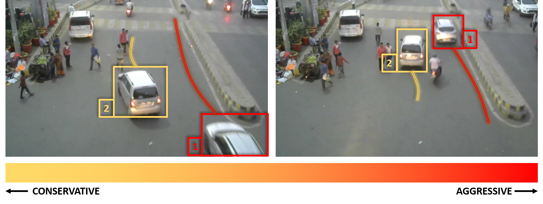
Figure 4: GraphRQI Performance: GraphRQI classifies road-agent 1 (red bounding box) as threatening and road-agent 2 (yellow bounding box) as conservative. We plot the vector, $w=\mathcal{L}u$, where $u$ is the eigenvector corresponding to the largest eigenvalue of $\mathcal{L}$, as a gradient below the figure.

V-D Ablation Experiments

Running Time Evaluation

For fair evaluation, we use the same programming platform (Python 3.7) and the same processor for running all the different methods (8 Core Intel Xeon(R) W2123 CPU clocked at 3.60GHz with 32 GB RAM). We empirically validate the theoretical guarantees of Theorem Lemma by replacing our eigenvalue algorithm with several standard eigenvector algorithms, Singular Value Decomposition (SVD), Incremental SVD[54], Restart SVD [53], Truncated SVD, and the state-of-the-art iterative method Conjugate Gradient Descent [27]. For SVD, and TruncatedSVD, we directly used the library routine implemented in the scipy package, and for RestartSVD, we used the authors’ original implementation. In practice, our method outperforms all these standard methods for Driver Behavior Classification. These results are shown in Table III.

Accuracy Evaluation

GraphRQI algorithm uses MLP for the final driver behavior classification. We replace this classifier with logistic regression, support vector machines (SVM [64])) and deep neural networks (LSTM [65]) and compare the results in Table III.

V-E Driver Behavior-Based Road-Agent Trajectory Prediction

We show that learning driver behavior can benefit road-agent navigation by improved trajectory prediction for each road-agent. Specifically, we demonstrate an application where knowledge of the behavior of a road-agent allows nearby road-agents to generate more efficient or safe paths. At any time-step $t$, given the coordinates of all road-agents and their corresponding behavior labels, we show that for the next $t+\Delta t$ seconds, aggressive (impatient, reckless, threatening) drivers may attempt to reach their goals faster through either overtaking, overspeeding, weaving, or tailgating. We also show that conservative (timid, cautious, careful) vehicles may steer away from aggressive road-agents. Our application is currently limited to straight road and four-way intersection networks. When moving through the network, each vehicle’s speed is computed using a car-following model [66]. The vehicles are parametrized using their positions, velocities, starting, and estimated short-term goal positions. Each vehicle is assigned a behavioral label through our behavior classification algorithm. Then as per the car-following model, the trajectories of the road agents are predicted. We include a demonstration of the application in the supplementary video.

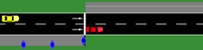
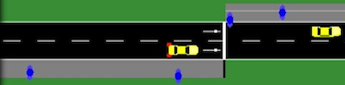
Figure 5: Trajectory Prediction Application: (top) We see an aggressive vehicle (red) cutting across a pedestrian, not allowing it to cross first. (bottom) Conservative vehicles, on the other hand, stop and wait for the pedestrian to cross first.

VI Conclusion, Limitations, and Future Work

We present a novel algorithm, GraphRQI, that can classify driver behaviors of road-agents from their trajectories. Our classification of behaviors is based on prior studies in traffic psychology, and our approach is designed for trajectory data from videos or other visual sensors. We compute the traffic matrices from the road-agent positions and use an eigenvalue algorithm to compute the spectrum of the Laplacian matrix. The spectrum comprises of the features used to train a multi-layer perceptron for driver behavior classification. We also present a faster algorithm to compute the eigenvalue and demonstrate the performance of our algorithm on two open-source traffic datasets. We observe $25\%$ improvement in classification over prior methods.

Our approach has some limitations. The accuracy of our approach is governed by the accuracy of the tracking methods used to compute the positions of the road-agent. While the spectrum of the traffic graph can be used to classify many behaviors, it may not be sufficient to classify the behaviors in all traffic scenarios. As part of future work, we also need to evaluate our algorithms on other traffic datasets. One major issue is the lack of sufficient labeled datasets in terms of driver behaviors. We would also like to combine the current approach with other deep learning models in order to improve accuracy and performance.

VII Acknowledgements

This work was supported in part by ARO Grants W911NF1910069 and W911NF1910315, Semiconductor Research Corporation (SRC), and Intel.

Appendix A Proof of Theorem IV.1

Theorem.

Given a sequence, $\{\mathcal{L}_{1},\mathcal{L}_{2},\ldots,\mathcal{L}_{T}\}$, our eigenvalue algorithm for $\mathcal{L}_{t}$ converges cubically with a running time complexity of $\mathcal{O}(\lvert\mathcal{L}^{\scriptscriptstyle-1}_{t}\rvert k)$ for each Laplacian at time-step $t$, where $k\ll\textnormal{dim}(\mathcal{L}_{t})$, with a storage cost of $\mathcal{O}(d)$.

Proof.

Our eigenvalue algorithm is motivated from the Rayleigh Quotient Iteration algorithm [59] (RQI). In RQI, to compute the eigenvector of any given matrix, $A$, corresponding to an approximation to a given eigenvalue, say $\eta$, the standard update formula for the RQI method is given as $x_{\textrm{new}}=(A-\eta I)^{-1}x_{\textrm{old}}$, where $x_{\textrm{old}}\in\mathbb{R}^{d\times 1}$ is initialized as a random vector. The efficiency of the update step depends on the efficiency of computing $(A-\eta I)^{-1}$. In GraphRQI, denoting $m=\lvert\mathcal{L}_{t}^{\scriptscriptstyle-1}\rvert$ as the number of non-zero elements of $\mathcal{L}_{t}^{\scriptscriptstyle-1}$, and $d=\textrm{dim}\mathcal{L}_{t}$, for each of the $k$ eigenvectors, the iterative update formula is: $x_{\textrm{new}}=(\mathcal{L}_{t}-\mu I)^{-1}x_{\textrm{old}}$. At first glance, it seems as if this update can be performed by applying the Sherman-Morrison (SM) update on the following decomposition:

$$(\mathcal{L}_{t}-\mu I)^{-1}=\left[\mathcal{L}_{t}-\mu\left(I_{1}+I_{2}+\ldots+I_{d}\right)\right]^{-1}$$ (4)

That is, by expressing $\mu I$ as a sum of $d$ rank-1 matrices, $I_{j}$, where each $I_{j}$ is a diagonal matrix with $I(j,j)=1$ and $0$ elsewhere. However, SM on $\mathcal{L}_{t}$ in the above equation requires $\mathcal{O}(d^{3})$ flops ($d^{2}$ flops for each SM operation applied $d$ times. See Lemma C). Therefore, we look towards a better solution.

Observe that we can decompose $\mathcal{L}_{t}=\mathcal{L}_{t}^{{}^{\prime}}+rr^{\top}$, where $\mathcal{L}_{t}^{{}^{\prime}}=\left[\begin{array}[]{c|c}\mathcal{L}^{r}_{t-1}\rule[-5.59721pt]{0.0pt}{0.0pt}&0\rule[-5.59721pt]{0.0pt}{0.0pt}\\ \hline\cr 0\rule{0.0pt}{11.19443pt}&1\end{array}\right]$ and $rr^{\top}$ is an outer product of rank 2 with $r\in\mathbb{R}^{d\times 2}$ is a vector of 1’s and 0’s, where $r(j)=1$ represents the addition of a new neighbor by the $j^{\textrm{th}}$ road-agent. $\mathcal{L}^{r}_{t-1}$ denotes the laplacian matrix at the previous time-step plus a diagonal update on account of observing $r$ new neighbors at the current time-step (This is further explained in lemma IV.2). So,

$$(\mathcal{L}_{t}-\mu I)^{-1}=(\mathcal{L}_{t}^{{}^{\prime}}+rr^{\top}-\mu I)^{-1},$$

where $rr^{\top}$ is a sum of two rank-1 matrices. Therefore, if we can compute $(\mathcal{L}_{t}^{{}^{\prime}}-\mu I)^{-1}$ in less than or equal to $\mathcal{O}(m)$, we are done. It is easy to verify that for any matrix $A$,

$$\left[\begin{array}[]{c|c}A\rule[-5.59721pt]{0.0pt}{0.0pt}&0\rule[-5.59721pt]{0.0pt}{0.0pt}\\ \hline\cr 0\rule{0.0pt}{11.19443pt}&1\end{array}\right]^{-1}=\left[\begin{array}[]{c|c}A^{-1}\rule[-5.59721pt]{0.0pt}{0.0pt}&0\rule[-5.59721pt]{0.0pt}{0.0pt}\\ \hline\cr 0\rule{0.0pt}{11.19443pt}&1\end{array}\right].$$

Therefore,

$$\left(\mathcal{L}_{t}^{{}^{\prime}}\right)^{\scriptscriptstyle-1}=\left[\begin{array}[]{c|c}\mathcal{L}^{r}_{t-1}\rule[-5.59721pt]{0.0pt}{0.0pt}&0\rule[-5.59721pt]{0.0pt}{0.0pt}\\ \hline\cr 0\rule{0.0pt}{11.19443pt}&1\end{array}\right]^{-1}=\left[\begin{array}[]{c|c}\left(\mathcal{L}^{r}_{t-1}\right)^{\scriptscriptstyle-1}\rule[-5.59721pt]{0.0pt}{0.0pt}&0\rule[-5.59721pt]{0.0pt}{0.0pt}\\ \hline\cr 0\rule{0.0pt}{11.19443pt}&1\end{array}\right]$$

and thus,

$$(\mathcal{L}_{t}^{{}^{\prime}}-\mu I)^{-1}=\left[\begin{array}[]{c|c}\left(\mathcal{L}^{r}_{t-1}-\mu I\right)^{\scriptscriptstyle-1}\rule[-5.59721pt]{0.0pt}{0.0pt}&0\rule[-5.59721pt]{0.0pt}{0.0pt}\\ \hline\cr 0\rule{0.0pt}{11.19443pt}&(1-\mu)\end{array}\right].$$

We can now use Lemma IV.2 to show that computing the inverse of the laplacian, $\left(\mathcal{L}^{r}_{t-1}-\mu I\right)$ can be performed in $\mathcal{O}(m)$. The entire update can be summarized as follows,

$\sigma\sigma^{\top}=\Sigma$.

At each time-step, we add a new column and a row to the laplacian matrix of the previous time-step. Therefore, the space complexity grows linearly with the dimension of the laplacian matrix. Finally, the cubic convergence follows from the classic RQI algorithm [59].

∎

Appendix B Proof of Lemma IV.2

Lemma.

The complexity of computing the inverse of a Laplacian at time-step $t$ grows as $\mathcal{O}(m)$.

Proof.

Note that $\mathcal{L}^{r}_{t-1}\neq\mathcal{L}_{t-1}\implies\left(\mathcal{L}^{r}_{t-1}\right)^{\scriptscriptstyle-1}\neq\mathcal{L}_{t-1}^{\scriptscriptstyle-1}$ since the diagonal elements (the degree of each node (vehicle)) are now different due the entry of new nodes at current time $t$. Let the number of new nodes be $r$. For example, if at the current time-step, 10 cars from the previous time-step observed a new neighbor, then $r=10$. Since we heuristically set the time-step and the KNN parameters, we constrain each vehicle observing at most 1 new neighbor for each time-step. Therefore,

$$\mathcal{L}^{r}_{t-1}=\mathcal{L}_{t-1}+\Sigma,$$

where $\Sigma=I_{1}+I_{2}+\ldots+I_{r}$ is a low-rank matrix with rank $r\ll d$, where we treat $r$ as a constant due to our earlier assumption. Each $I_{j}$ is a diagonal matrix with $I(j,j)=1$ and $0$ elsewhere. Hence,

$$\begin{split}\left(\mathcal{L}^{r}_{t-1}-\mu I\right)&=\mathcal{L}_{t-1}-\mu I+\Sigma\\ \left(\mathcal{L}^{r}_{t-1}-\mu I\right)^{\scriptscriptstyle-1}&=\left(\mathcal{L}_{t-1}-\mu I+I_{1}+I_{2}+\ldots+I_{r}\right)^{-1},\\ \end{split}$$ (6)

where $(\mathcal{L}_{t-1}-\mu I)^{-1}=U_{t-1}(\Lambda-\mu I)^{\scriptscriptstyle-1}U_{t-1}^{\top}$. Using the Sherman-Morrison formula $r$ times on $(\mathcal{L}_{t-1}-\mu I)$, we get $\left(\mathcal{L}^{r}_{t-1}-\mu I\right)^{\scriptscriptstyle-1}$ in $\mathcal{O}(m)$ (See appendix C).

∎

Appendix C Lemma 3: Each Sherman-Morrison operation requires $\mathcal{O}(m)$ flops.

Proof.

For a matrix of size $d\times d$, each SM operation requires,

• 2 matrix-vector multiplications - $\mathcal{O}(m)$

• 1 inner product - $\mathcal{O}(m)$

• 1 outer-product computation - $\mathcal{O}(m)$

• 1 matrix subtraction - $\mathcal{O}(m)$

∎

Appendix D Annotation of TRAF and Argoverse Datasets

We study and classify road-agents into six different driving behaviors. We used two datasets for training a neural network and the class-wise distribution of the final labels are shown in Figure 6.

Label	Traits
Impatient	Overtaking
	Over-speeding
	Tailgating
	Weaving
Threatening	Cutting in front of agents
	Driving extremely close to agents
Reckless	Driving in the wrong direction
	Jaywalking through traffic
	Not following rules
Careful	Maintain neighbors
	Uniform Speed
	Follow rules
Timid	Not moving
	Slowing down/coming to stop
Cautious	Waiting for vehicles/pedestrians

Table V: Driver Behavior Traits.

Studies in traffic psychology show that each of the six driving behaviors are associated with certain driving traits. For example, impatient drivers show different traits (e.g., over-speeding, overtaking) than reckless drivers (e.g., driving in the opposite direction to the traffic) [25]. Similarly, timid drivers may drive slower than the speed limit [26], and careful drivers obey the traffic rules. We now describe the labeling process. First we distinguish between annotators and expert annotators. Annotators correspond to the individuals that labeled the videos via crowd-sourcing. They may or may not have expertise or familiarity with the traffic in the videos. All annotators were asked to observe these traits in the videos and list the most prominent traits observed in each road-agent. The trait table is shown in the Table V.

The annotators were not shown the class-wise distribution of traits, nor were they shown annotations marked by any other annotator. Each annotator was presented with a uniform presentation of traits and their task was to simply mark the traits that they observed for each vehicle. Each annotator labeled every video. The final class was assigned by resolving discrepancies for each road-agent. Some vehicles would receive conflicting traits. If the conflicting traits belonged to the same Parent class (aggressive or conservative), then we would simply select the majority trait. In rare scenarios where there is no majority, we would simply take a final call. However, if the conflicting traits belonged to different parent classes, then that road-agent would be re-annotated through crowd-sourcing, and would repeat the steps.

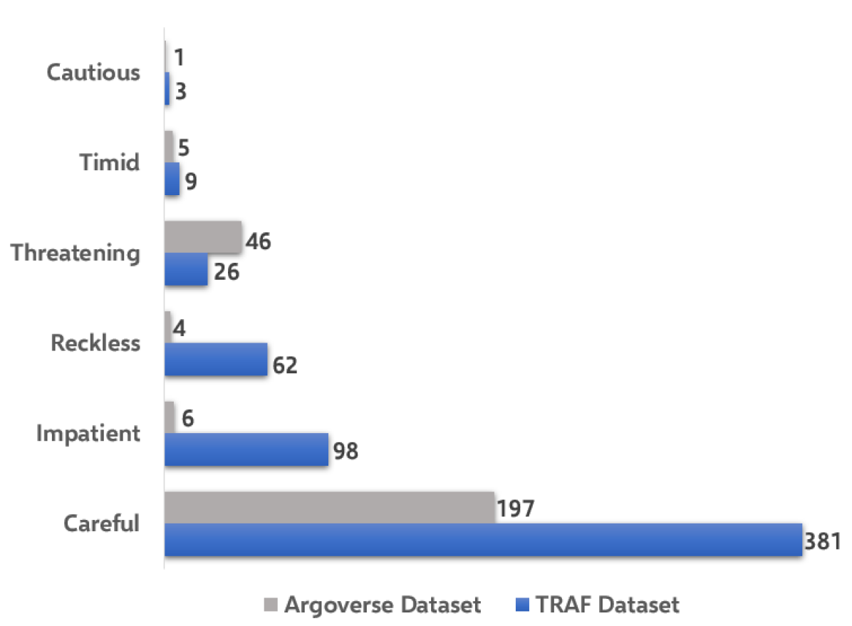
Figure 6: Class-wise distribution of the final labels

References

- [1] C. Badue, R. Guidolini, R. V. Carneiro, P. Azevedo, V. B. Cardoso, A. Forechi, L. F. R. Jesus, R. F. Berriel, T. M. Paixão, F. Mutz, et al., “Self-driving cars: A survey,” arXiv preprint arXiv:1901.04407, 2019.
- [2] W. Schwarting, J. Alonso-Mora, and D. Rus, “Planning and decision-making for autonomous vehicles,” Annual Review of Control, Robotics, and Autonomous Systems, 2018.
- [3] R. Chandra, U. Bhattacharya, T. Randhavane, A. Bera, and D. Manocha, “Roadtrack: Tracking road agents in dense and heterogeneous environments,” arXiv preprint arXiv:1906.10712, 2019.
- [4] R. Chandra, U. Bhattacharya, A. Bera, and D. Manocha, “Densepeds: Pedestrian tracking in dense crowds using front-rvo and sparse features,” arXiv preprint arXiv:1906.10313, 2019.
- [5] S. Pendleton, H. Andersen, X. Du, X. Shen, M. Meghjani, Y. Eng, D. Rus, and M. Ang, “Perception, planning, control, and coordination for autonomous vehicles,” Machines, vol. 5, no. 1, p. 6, 2017.
- [6] W. Schwarting, J. Alonso-Mora, and D. Rus, “Planning and decision-making for autonomous vehicles,” Annual Review of Control, Robotics, and Autonomous Systems, 2018.
- [7] A. Alahi, K. Goel, V. Ramanathan, A. Robicquet, L. Fei-Fei, and S. Savarese, “Social lstm: Human trajectory prediction in crowded spaces,” in Proceedings of the IEEE Conference on Computer Vision and Pattern Recognition, 2016, pp. 961–971.
- [8] A. Gupta, J. Johnson, L. Fei-Fei, S. Savarese, and A. Alahi, “Social GAN: Socially Acceptable Trajectories with Generative Adversarial Networks,” ArXiv e-prints, Mar. 2018.
- [9] R. Chandra, U. Bhattacharya, A. Bera, and D. Manocha, “Traphic: Trajectory prediction in dense and heterogeneous traffic using weighted interactions,” in Proceedings of the IEEE Conference on Computer Vision and Pattern Recognition, 2019, pp. 8483–8492.
- [10] R. Chandra, U. Bhattacharya, C. Roncal, A. Bera, and D. Manocha, “Robusttp: End-to-end trajectory prediction for heterogeneous road-agents in dense traffic with noisy sensor inputs,” arXiv preprint arXiv:1907.08752, 2019.
- [11] R. Chandra, T. Guan, S. Panuganti, T. Mittal, U. Bhattacharya, A. Bera, and D. Manocha, “Forecasting trajectory and behavior of road-agents using spectral clustering in graph-lstms,” arXiv preprint arXiv:1912.01118, 2019.
- [12] E. Cheung, A. Bera, E. Kubin, K. Gray, and D. Manocha, “Identifying driver behaviors using trajectory features for vehicle navigation,” in 2018 IEEE/RSJ International Conference on Intelligent Robots and Systems (IROS). IEEE, 2018, pp. 3445–3452.
- [13] E. Cheung, A. Bera, and D. Manocha, “Efficient and safe vehicle navigation based on driver behavior classification,” in Proceedings of the IEEE Conference on Computer Vision and Pattern Recognition Workshops, 2018, pp. 1024–1031.
- [14] B. Paden, M. Čáp, S. Z. Yong, D. Yershov, and E. Frazzoli, “A survey of motion planning and control techniques for self-driving urban vehicles,” IEEE Transactions on intelligent vehicles, vol. 1, no. 1, pp. 33–55, 2016.
- [15] J. Hong, B. Sapp, and J. Philbin, “Rules of the road: Predicting driving behavior with a convolutional model of semantic interactions,” in The IEEE Conference on Computer Vision and Pattern Recognition (CVPR), June 2019.
- [16] V. Ramanishka, Y.-T. Chen, T. Misu, and K. Saenko, “Toward driving scene understanding: A dataset for learning driver behavior and causal reasoning,” in Proceedings of the IEEE Conference on Computer Vision and Pattern Recognition, 2018, pp. 7699–7707.
- [17] L. Sun, W. Zhan, C.-Y. Chan, and M. Tomizuka, “Behavior planning of autonomous cars with social perception,” arXiv preprint arXiv:1905.00988, 2019.
- [18] X. Geng, H. Liang, B. Yu, P. Zhao, L. He, and R. Huang, “A scenario-adaptive driving behavior prediction approach to urban autonomous driving,” Applied Sciences, vol. 7, no. 4, p. 426, 2017.
- [19] R. Hoogendoorn, B. van Arerm, and S. Hoogendoom, “Automated driving, traffic flow efficiency, and human factors: Literature review,” Transportation Research Record, vol. 2422, no. 1, pp. 113–120, 2014.
- [20] R. Yoshizawa, Y. Shiomi, N. Uno, K. Iida, and M. Yamaguchi, “Analysis of car-following behavior on sag and curve sections at intercity expressways with driving simulator,” International Journal of Intelligent Transportation Systems Research, vol. 10, no. 2, pp. 56–65, 2012.
- [21] M. Saifuzzaman and Z. Zheng, “Incorporating human-factors in car-following models: a review of recent developments and research needs,” Transportation research part C: emerging technologies, vol. 48, pp. 379–403, 2014.
- [22] J. Rong, K. Mao, and J. Ma, “Effects of individual differences on driving behavior and traffic flow characteristics,” Transportation research record, vol. 2248, no. 1, pp. 1–9, 2011.
- [23] J. Warren, J. Lipkowitz, and V. Sokolov, “Clusters of driving behavior from observational smartphone data,” IEEE Intelligent Transportation Systems Magazine, vol. 11, no. 3, pp. 171–180, 2019.
- [24] E. R. Dahlen, B. D. Edwards, T. Tubré, M. J. Zyphur, and C. R. Warren, “Taking a look behind the wheel: An investigation into the personality predictors of aggressive driving,” Accident Analysis & Prevention, vol. 45, pp. 1–9, 2012.
- [25] B. McNally and G. L. Bradley, “Re-conceptualising the reckless driving behaviour of young drivers,” Accident Analysis & Prevention, vol. 70, pp. 245–257, 2014.
- [26] R. Cheng, H. Ge, and J. Wang, “An extended continuum model accounting for the driver’s timid and aggressive attributions,” Physics Letters A, vol. 381, no. 15, pp. 1302–1312, 2017.
- [27] J. R. Shewchuk et al., “An introduction to the conjugate gradient method without the agonizing pain,” 1994.
- [28] M.-F. Chang, J. Lambert, P. Sangkloy, J. Singh, S. Bak, A. Hartnett, D. Wang, P. Carr, S. Lucey, D. Ramanan, and J. Hays, “Argoverse: 3d tracking and forecasting with rich maps,” in The IEEE Conference on Computer Vision and Pattern Recognition (CVPR), June 2019.
- [29] Z. Wei-hua, “Selected model and sensitivity analysis of aggressive driving behavior,” 2012.
- [30] M. R. Barrick and M. K. Mount, “The big five personality dimensions and job performance: a meta-analysis,” Personnel psychology, vol. 44, no. 1, pp. 1–26, 1991.
- [31] A. Aljaafreh, N. Alshabatat, and M. S. N. Al-Din, “Driving style recognition using fuzzy logic,” 2012 IEEE International Conference on Vehicular Electronics and Safety (ICVES 2012), pp. 460–463, 2012.
- [32] B. Krahé and I. Fenske, “Predicting aggressive driving behavior: The role of macho personality, age, and power of car,” Aggressive Behavior: Official Journal of the International Society for Research on Aggression, vol. 28, no. 1, pp. 21–29, 2002.
- [33] K. H. Beck, B. Ali, and S. B. Daughters, “Distress tolerance as a predictor of risky and aggressive driving.” Traffic injury prevention, vol. 15 4, pp. 349–54, 2014.
- [34] J. C. Brill, M. Mouloua, E. Shirkey, and P. Alberti, “Predictive validity of the aggressive driver behavior questionnaire (adbq) in a simulated environment,” in Proceedings of the Human Factors and Ergonomics Society Annual Meeting, vol. 53, no. 18. SAGE Publications Sage CA: Los Angeles, CA, 2009, pp. 1334–1337.
- [35] Y. L. Murphey, R. Milton, and L. Kiliaris, “Driver’s style classification using jerk analysis,” 2009 IEEE Workshop on Computational Intelligence in Vehicles and Vehicular Systems, pp. 23–28, 2009.
- [36] I. Mohamad, M. A. M. Ali, and M. Ismail, “Abnormal driving detection using real time global positioning system data,” Proceeding of the 2011 IEEE International Conference on Space Science and Communication (IconSpace), pp. 1–6, 2011.
- [37] G. Qi, Y. Du, J. Wu, and M. Xu, “Leveraging longitudinal driving behaviour data with data mining techniques for driving style analysis,” IET intelligent transport systems, vol. 9, no. 8, pp. 792–801, 2015.
- [38] B. Shi, L. Xu, J. Hu, Y. Tang, H. Jiang, W. Meng, and H. Liu, “Evaluating driving styles by normalizing driving behavior based on personalized driver modeling,” IEEE Transactions on Systems, Man, and Cybernetics: Systems, vol. 45, pp. 1502–1508, 2015.
- [39] W. Wang, J. Xi, A. Chong, and L. Li, “Driving style classification using a semisupervised support vector machine,” IEEE Transactions on Human-Machine Systems, vol. 47, pp. 650–660, 2017.
- [40] D. Sadigh, K. R. Driggs-Campbell, A. Puggelli, W. Li, V. Shia, R. Bajcsy, A. L. Sangiovanni-Vincentelli, S. S. Sastry, and S. A. Seshia, “Data-driven probabilistic modeling and verification of human driver behavior,” in AAAI Spring Symposia, 2014.
- [41] S. Qi and S.-C. Zhu, “Intent-aware multi-agent reinforcement learning,” in 2018 IEEE International Conference on Robotics and Automation (ICRA). IEEE, 2018, pp. 7533–7540.
- [42] F. Codevilla, M. Miiller, A. López, V. Koltun, and A. Dosovitskiy, “End-to-end driving via conditional imitation learning,” in 2018 IEEE International Conference on Robotics and Automation (ICRA). IEEE, 2018, pp. 1–9.
- [43] A. Zyner, S. Worrall, and E. Nebot, “A recurrent neural network solution for predicting driver intention at unsignalized intersections,” IEEE Robotics and Automation Letters, vol. 3, no. 3, pp. 1759–1764, 2018.
- [44] A. Zyner, S. Worrall, J. Ward, and E. Nebot, “Long short term memory for driver intent prediction,” in 2017 IEEE Intelligent Vehicles Symposium (IV). IEEE, 2017, pp. 1484–1489.
- [45] H. Yeh, S. Curtis, S. Patil, J. van den Berg, D. Manocha, and M. Lin, “Composite agents,” in Proceedings of the 2008 ACM SIGGRAPH/Eurographics Symposium on Computer Animation, 2008, pp. 39–47.
- [46] D. Helbing and P. Molnar, “Social force model for pedestrian dynamics,” Physical review E, vol. 51, no. 5, p. 4282, 1995.
- [47] A. Bera, S. Kim, T. Randhavane, S. Pratapa, and D. Manocha, “Glmp-realtime pedestrian path prediction using global and local movement patterns,” in 2016 IEEE International Conference on Robotics and Automation (ICRA). IEEE, 2016, pp. 5528–5535.
- [48] A. Bera, S. Kim, and D. Manocha, “Realtime anomaly detection using trajectory-level crowd behavior learning,” in Proceedings of the IEEE Conference on Computer Vision and Pattern Recognition Workshops, 2016, pp. 50–57.
- [49] S. J. Guy, J. Van Den Berg, W. Liu, R. Lau, M. C. Lin, and D. Manocha, “A statistical similarity measure for aggregate crowd dynamics,” ACM Transactions on Graphics (TOG), vol. 31, no. 6, pp. 1–11, 2012.
- [50] J. Bruna, W. Zaremba, A. Szlam, and Y. LeCun, “Spectral networks and locally connected networks on graphs,” arXiv preprint arXiv:1312.6203, 2013.
- [51] T. N. Kipf and M. Welling, “Semi-supervised classification with graph convolutional networks,” arXiv preprint arXiv:1609.02907, 2016.
- [52] B. Yu, H. Yin, and Z. Zhu, “Spatio-temporal graph convolutional networks: A deep learning framework for traffic forecasting,” arXiv preprint arXiv:1709.04875, 2017.
- [53] Z. Zhang, P. Cui, J. Pei, X. Wang, and W. Zhu, “Timers: Error-bounded svd restart on dynamic networks,” in Thirty-Second AAAI Conference on Artificial Intelligence, 2018.
- [54] M. Brand, “Fast low-rank modifications of the thin singular value decomposition,” Linear algebra and its applications, vol. 415, no. 1, pp. 20–30, 2006.
- [55] J. Li, H. Dani, X. Hu, J. Tang, Y. Chang, and H. Liu, “Attributed network embedding for learning in a dynamic environment,” in Proceedings of the 2017 ACM on Conference on Information and Knowledge Management. ACM, 2017, pp. 387–396.
- [56] M. Belkin and P. Niyogi, “Laplacian eigenmaps for dimensionality reduction and data representation,” Neural computation, vol. 15, no. 6, pp. 1373–1396, 2003.
- [57] W. Stallings, Data and computer communications. Pearson Education India, 2007.
- [58] N. S. Altman, “An introduction to kernel and nearest-neighbor nonparametric regression,” The American Statistician, vol. 46, no. 3, pp. 175–185, 1992.
- [59] J. W. Demmel, Applied numerical linear algebra. Siam, 1997, vol. 56.
- [60] W. W. Hager, “Updating the inverse of a matrix,” SIAM review, vol. 31, no. 2, pp. 221–239, 1989.
- [61] V. V. Williams, “Multiplying matrices in o (n2. 373) time,” 2014.
- [62] M. W. Gardner and S. Dorling, “Artificial neural networks (the multilayer perceptron)—a review of applications in the atmospheric sciences,” Atmospheric environment, vol. 32, no. 14-15, pp. 2627–2636, 1998.
- [63] J. Li, H. Dani, X. Hu, J. Tang, Y. Chang, and H. Liu, “Attributed network embedding for learning in a dynamic environment,” in Proceedings of the 2017 ACM on Conference on Information and Knowledge Management. ACM, 2017, pp. 387–396.
- [64] C. Cortes and V. Vapnik, “Support-vector networks,” Machine learning, vol. 20, no. 3, pp. 273–297, 1995.
- [65] S. Hochreiter and J. Schmidhuber, “Long short-term memory,” Neural computation, vol. 9, no. 8, pp. 1735–1780, 1997.
- [66] S. Krauss, “Microscopic modeling of traffic flow: Investigation of collision free vehicle dynamics,” Ph.D. dissertation, 1998.