Non-Gaussian processes and neural networks at finite widths
Abstract
Gaussian processes are ubiquitous in nature and engineering. A case in point is a class of neural networks in the infinite-width limit, whose priors correspond to Gaussian processes. Here we perturbatively extend this correspondence to finite-width neural networks, yielding non-Gaussian processes as priors. The methodology developed herein allows us to track the flow of preactivation distributions by progressively integrating out random variables from lower to higher layers, reminiscent of renormalization-group flow. We further develop a perturbative procedure to perform Bayesian inference with weakly non-Gaussian priors.
I Inception
Gaussian processes model many phenomena in the physical world. A prime example is Brownian motion Brown (1828), modeled as the integral of Gaussian-distributed bumps exerted on a point-like solute Einstein (1905). The theory of elementary particles Weinberg (1995) also becomes a Gaussian process in the free limit where interactions between particles are turned off, and many-body systems as complex as glasses come to be Gaussian in the infinite-dimensional, mean-field, limit Parisi and Zamponi (2010). In the context of machine learning, Neal in Ref. Neal (1996) pointed out that a class of neural networks give rise to Gaussian processes in the infinite-width limit, which can perform exact Bayesian inference from training to test data Williams (1997). They occupy a corner of theoretical playground wherein the karakuri of neural networks is scrutinized Lee et al. (2018); Matthews et al. (2018); Jacot et al. (2018); Chizat et al. (2018); Lee et al. (2019); Geiger et al. (2019).
In reality, Gaussian processes are but mere idealizations. Brownian particles have finite-size structure, elementary particles interact, and many-body systems respond nonlinearly. In order to understand rich phenomena exhibited by these real systems, Gaussian processes rather serve as starting points to be perturbed around. Indeed many edifices in theoretical physics are built upon the successful treatment of non-Gaussianity, with a notable example being renormalization-group flow Kadanoff (1966); Wilson (1971); Weinberg (1996); Goldenfeld (2018). In the quest to elucidate behaviors of real neural networks away from the infinite-width limit, it is thus natural to wonder if the similar treatment of non-Gaussianity yields equally elegant and powerful machinery.
Here we set out on this program, perturbatively treating finite-width corrections to neural networks. Prior distributions of outputs are obtained through progressively integrating out preactivations of neurons layer by layer, yielding non-Gaussian priors. The whole procedure closely resembles renormalization-group flow Goldenfeld (2018); Mehta and Schwab (2014): it bridges probability distributions at different scales through coarse-graining of random variables at microscopic scales; the flow of distributions is traced through running couplings, which in particular capture the degree of non-Gaussianity in these distributions; resulting recursive equations (R1,R2,R3) govern the evolution of these running couplings from lower to higher layers, just as renormalization-group equations do from microscopic to macroscopic scales. Such a recursive approach enables us to treat finite-width corrections to various observables, for networks with arbitrary activation functions.
The rest of the paper is structured as follows. In Section II we review and set up basic concepts. Our master recursive formulae (R1,R2,R3) are derived in Section III, which control the flow of preactivation distributions. After an interlude with concrete examples in Section IV, we extend the Gaussian-process Bayesian inference to non-Gaussian priors in Section V and study inference of neural networks at finite widths. We conclude in Section VI with dreams.
II To infinity and beyond
In this paper we study real finite-width neural networks in the regime where the number of neurons in hidden layers is asymptotically large whereas input and output dimensions are kept constant.
II.1 Gaussian processes and neural networks at infinite widths
Let us focus on a class of neural networks termed multilayer perceptrons, with model parameters, , and an activation function, . For each input, , a neural network outputs a vector, , recursively defined as sequences of preactivations through
| (1) | |||||
| (2) |
Following Ref. Neal (1996), we assume priors for biases and weights given by independent and identically distributed Gaussian distributions with zero means, , and variances
| (3) | |||||
| (4) |
Higher moments are then obtained by Wick’s contractions Wick (1950); Zee (2010). For instance,
| (5) |
For those unfamiliar with Wick’s contractions and connected correlation functions (a.k.a. cumulants), a pedagogical review is provided in Appendix A as our formalism heavily relies on them.
In the infinite-width limit where (but finite and ), it has been argued – with varying degrees of rigor Neal (1996); Lee et al. (2018); Matthews et al. (2018) – that the prior distribution of outputs is governed by the Gaussian process with a kernel
| (6) |
and all the higher moments given by Wick’s contractions. Here, the sample index labels different inputs in a dataset. There exists a recursive formula that lets us evaluate this kernel for any pair of inputs Lee et al. (2018) [c.f. Equation (R1)]. Importantly, once the values of the kernel are evaluated for all the pairs of input data, , consisting of training inputs with target outputs and test inputs with unknown targets, we can perform exact Bayesian inference to yield mean outputs as predictions for test data Williams (1997); Williams and Rasmussen (2006) [c.f. Equation (GPM)]. This should be contrasted with stochastic gradient descent (SGD) optimization Robbins and Monro (1951), through which typically a single estimate for the optimal model parameters of the posterior, , is obtained and used to predict outputs for test inputs; Bayesian inference instead marginalizes over all model parameters, performing an ensemble average over the posterior distribution MacKay (1995).
II.2 Beyond infinity
We shall now study real finite-width neural networks in the regime .111Note that input and output dimensions, and , are arbitrary. To be precise, defining , we send while keeping , , , and constants, and compute the leading corrections. In particular it is crucial to keep the number of outputs constant in order to consistently perform Bayesian inference within our approach. At finite widths, there are corrections to Gaussian-process priors. In other words, a whole tower of nontrivial preactivation correlation functions beyond the kernel,
| (7) |
collectively dictate the distribution of preactivations. Our aim is to trace the flow of these distributions progressively and cumulatively all the way up to the last layer whereat Bayesian inference is executed. More specifically, we shall inductively and self-consistently show that two-point preactivation correlation functions take the form222In the main text we place tildes on objects that depend only on sample indices ’s in order to distinguish them from those that depend both on sample indices ’s and neuron indices ’s.
| (KS) |
and connected four-point preactivation correlation functions
| (V) | ||||
and higher cumulants are all suppressed by .333Given that the means of biases and weights are zero, for all odd . Here the Gaussian-process core kernel and the self-energy correction are symmetric under the exchange of sample indices and the four-point vertex is symmetric under , , and . At the first layer the preactivation distribution is exactly Gaussian for any finite widths and hence Equations (KS) and (V) are trivially satisfied, with
| (R0) |
Obtained in Section III are the recursive formulae that link these core kernel, self-energy, and four-point vertex at the -th layer to those at the -th layer while in Section V these tensors at the last layer are used to yield the leading correction for Bayesian inference at finite widths.
II.3 Related work
Our Schwinger operator approach is orthogonal to the replica approach by Cohen et al. (2019) and, unlike the planar diagrammatic approach by Dyer and Gur-Ari (2019), applies to general activation functions, made possible by accumulating corrections layer by layer rather than dealing with them all at once. See also Antognini (2019). More substantially, in contrast to these previous approaches, we here study finite-width effects on Bayesian inference and find that the renormalization-group picture naturally emerges, with layers playing the role of scales.
III Distributional flow
As auxiliary objects in recursive steps, let us introduce activation correlation functions
| (8) |
Our basic strategy is to establish relations
| (ZIGZAG) |
zigzagging between sets of preactivation correlation functions and sets of activation correlation functions, keeping track of leading finite-width corrections. Below, relations are obtained by integrating out preactivations while relations are obtained by integrating out biases and weights. At first glance the algebra in this paper may look horrifying but repeated applications of Wick’s contractions are all there is to it. The results are summarized in Section III.2.
III.1 Zigzag relations for preactivation and activation correlation functions
Integrating over the Gaussian biases and weights at ’s connections yield the relations that link activation correlations to preactivation correlations at the next layer. Recalling Equations (KS) and (V), trivial Wick’s contractions yield
| (9) | |||||
| (10) |
The remaining task is to relate preactivation correlations to activation correlations within the same layer, which will complete the zigzag relation (ZIGZAG) for these correlation functions.444The nontrivial parts of the inductive proof for Equations (KS) and (V) are to show (i) that the right-hand side of Equation (10) is finite as , (ii) that the leading contribution of Equation (9) is the Gaussian-process kernel, and (iii) that higher-point connected preactivation correlation functions are all suppressed by , all of which are verified in obtaining the recursive equations. See Appendix B for a full proof.
With the mastery of Wick’s contractions and connected correlation functions, it is simple to derive the following combinatorial hack (Appendix A.4): viewing prior preactivations
at the -th layer as a random -dimensional vector and defining the Gaussian integral with the kernel , the prior average
| (HACK) |
for any function . Here the operators and capture corrections due to self-energy and four-point vertex, respectively, and are defined as
| (OS) | ||||
| (OV) | ||||
where the sample indices are raised by using the inverse core kernel as a metric, meaning
| (11) | |||||
| (12) |
Using the above hack, we can evaluate the activation correlations by straightforward algebra with Wick’s contractions. In particular, as the Gaussian integral is diagonal in the neuron index , we just need to disentangle cases with repeated and unrepeated neuron indices. The solution for this exercise is in Appendix B: it is arguably the most cumbersome algebra in this paper.
III.2 Master recursive flow equations
Denoting the Gaussian integral with the core kernel for a single-neuron random vector , and plugging in results of Appendix B into Equations (9) and (10), we arrive at our master recursion relations
| (R1) | ||||
| (R2) | ||||
| (R3) | ||||
For , a special note about the ratio is in order: even though stays constant while , the terms proportional to that ratio are identically zero due to the complete Gaussianity (R0).
The preactivation distribution in the first layer (R0) sets the initial condition for the flow from lower to higher layers dictated by these recursive equations. Evolving through these recursive equations, the running couplings – , , and – then trace changes in the distributions of preactivations as the layer scale shifts, just as running couplings for physical systems track changes in effective Boltzmann distributions as the probing scale shifts. Once recursed up to the last layer , the resulting distribution of outputs can be succinctly encoded by the probability distribution
| (D0) |
with the potential where ,
| (D1) | ||||
| (D2) | ||||
| (13) |
Again, this can be derived through Wick’s contractions. It is important to note that is constant and thus can consistently be treated perturbatively.555If were of order , the potential would become a large- vector model, for which we would have to sum the infinite series of bubble diagrams Moshe and Zinn-Justin (2003).
IV Interlude: examples
The recursive relations obtained above can be evaluated numerically Lee et al. (2018) [or sometimes analytically for rectified linear unit (ReLU) activation Cho and Saul (2009)], which is a perfectly adequate approach: at the leading order it involves four-dimensional Gaussian integrals at most. Here, continuing the theme of wearing out Wick’s contractions, we develop an alternative analytic method that works for any polynomial activations Liao and Poggio (2017), providing another perfectly cromulent approach.
For a general polynomial activation of degree , , the nontrivial term in Equation (R1) can be expanded as
| (14) |
Each term can then be evaluated by Wick’s contractions and the same goes for all the terms in Equations (R2) and (R3).666The same approach could be adopted for an analytic function but it would in general be difficult to sum the resulting infinite series in a closed form. It could nonetheless be useful in, for example, proving convergence properties. Below and in Appendix C, we illustrate this procedure with simple examples.
IV.1 Deep linear networks
When the activation function is linear, , multilayer perceptrons are called deep linear networks Saxe et al. (2013). Setting and for simplicity, our recursion relations reduce to ,
and . Solving them yields the layer-independent core kernel and zero self-energy
| (15) |
and the linearly layer-dependent four-point vertex
| (16) |
It succinctly reproduces the result that can be obtained through planar diagrams in this special setup Dyer and Gur-Ari (2019). Quadratic activation Li et al. (2018) is worked out in Appendix C.1.
IV.2 ReLU with single input
The recursion relations simplify drastically for the case of a single input, , as worked out in detail in Appendix C.2. For instance, for ReLU activation with and , we obtain the layer-independent core kernel, zero self-energy, and the four-point vertex
| (17) |
Interestingly, as for deep linear networks, the factor appears again. This factor has also been found by Hanin and Rolnick (2018), which provides guidance for network architectural design through its minimization. We generalize this factor for monomial activations in Appendix C.2.1
IV.3 Experimental verification: output distributions for a single input
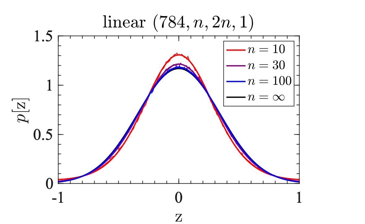
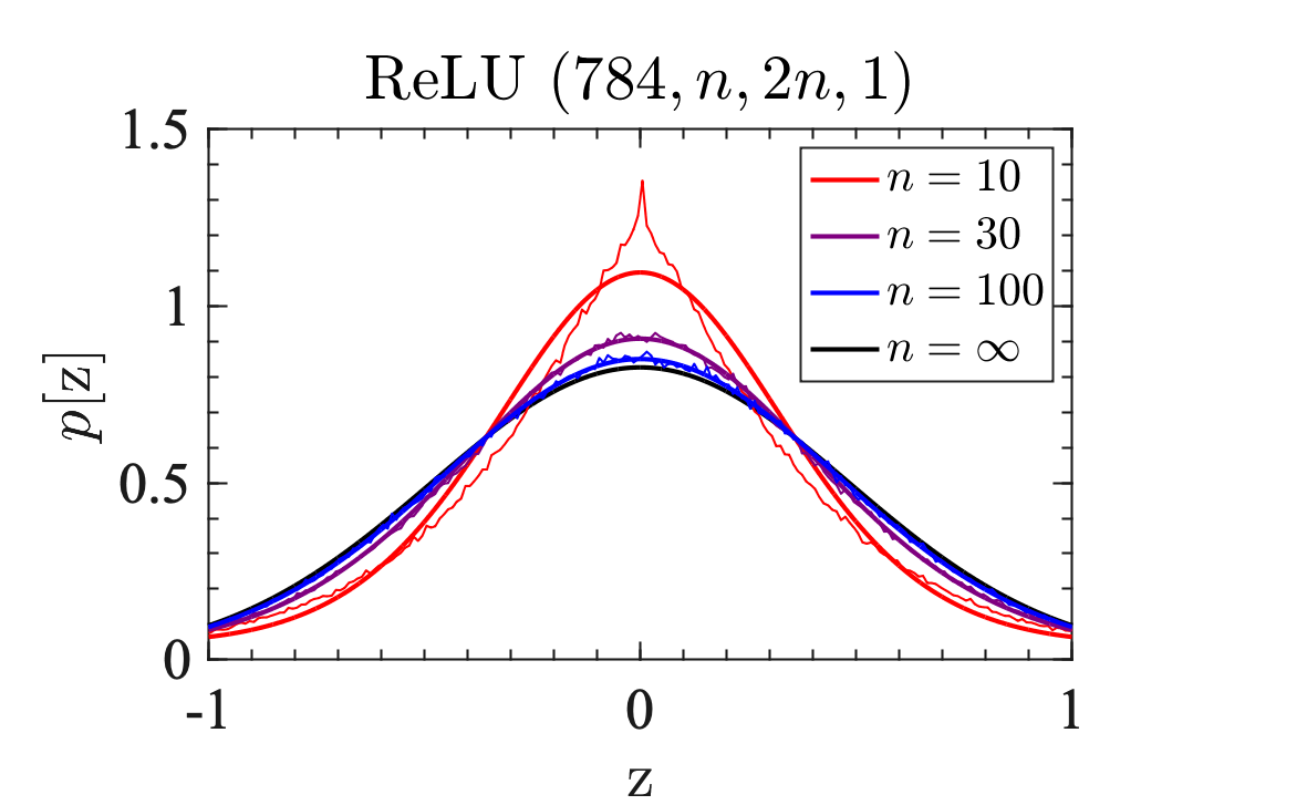
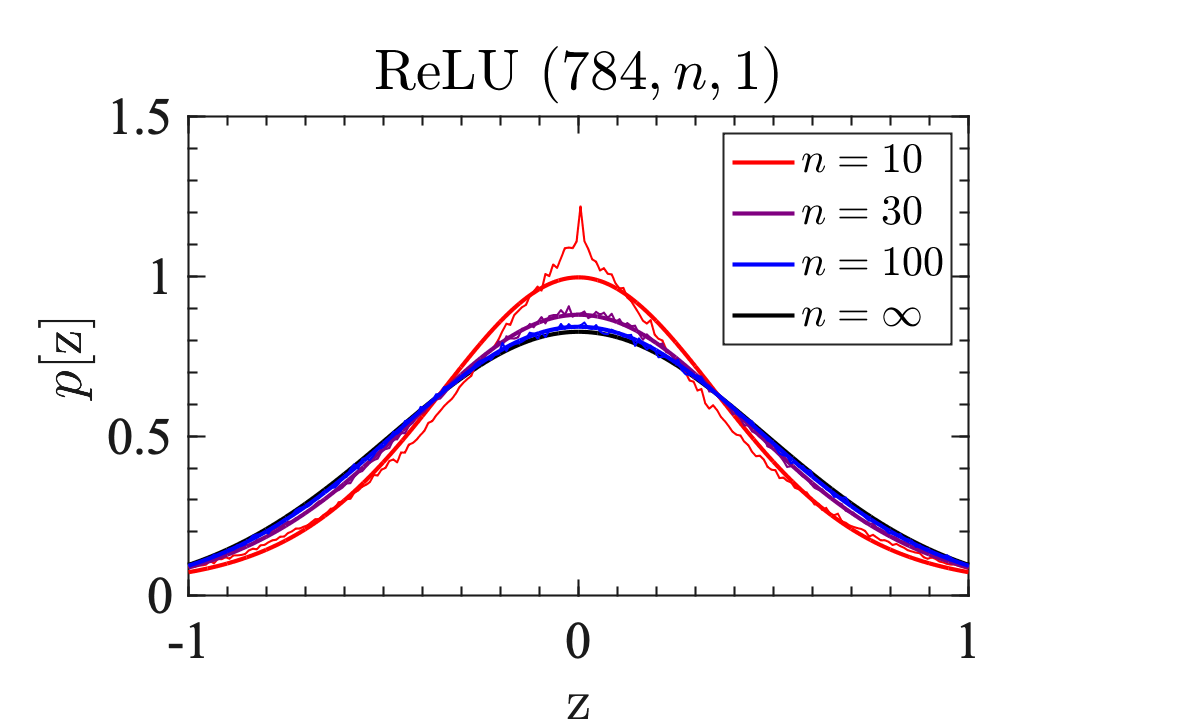
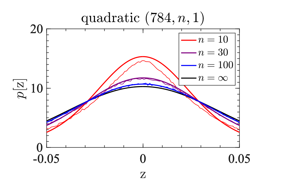
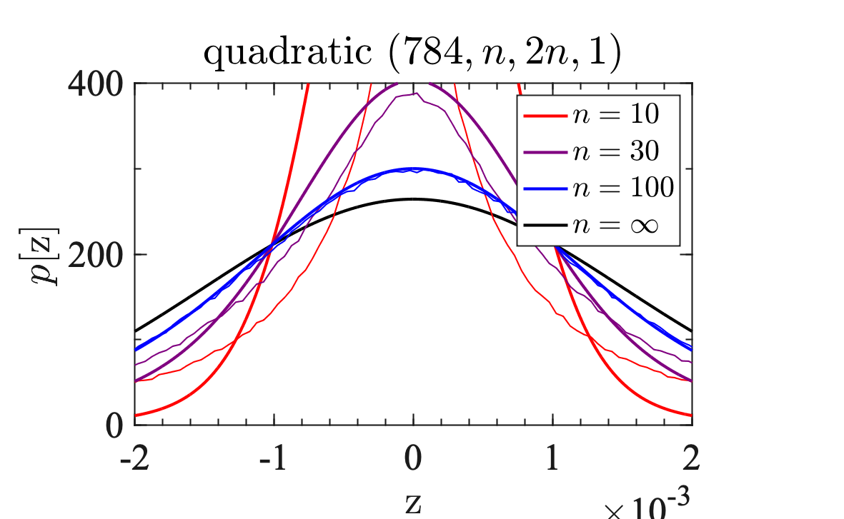
Here we put our theory to the test. For concreteness, take a single black-white image of hand-written digits with -by- pixels (i.e. ) from the MNIST dataset LeCun et al. (1998) without preprocessing, set depth , bias variance , weight variance , and widths , and use activations (linear) with and (ReLU) with . In Figure 1, for each width-parameter of the hidden layers we record the prior distribution of outputs over instances of Gaussian weights and compare it with the theoretical prediction – obtained by cranking the knob from the initial condition (R0) through the recursion relations (R1-R3) to the distribution (D0-D2). The prior distribution becomes increasingly non-Gaussian as networks narrow and the deviation from the Gaussian-process prior is correctly captured by our theory. Higher-order perturbative calculations are expected to systematically improve the quality – and extend the range – of the agreement. Additional experiments are performed in Appendix C.3, which further corroborates our theory.
V Bayesian inference
Let us take off from the terminal point of Section III: we have obtained the recursive equations (R0-R3) for the Gaussian-process kernel and the leading finite-width corrections and codified them in the weakly non-Gaussian prior distributions (D0-D2) of outputs
dictated by the potential with . Examples in Section IV illustrate that finite-width corrections stay perturbative typically when . Let us now divide inputs into training and test inputs as
| (18) |
and the training inputs come with target outputs
| (19) |
We shall develop a procedure to infer outputs for test inputs a lá Bayes, perturbatively extending the textbook Williams and Rasmussen (2006). For field theorists, our calculation is just a background-field calculation Weinberg (1996) in disguise.
Taking the liberty of notations, we let the number of input-data arguments dictate the summation over sample indices inside the potential , and denote the joint probabilities
| (20) |
Given the training targets , the posterior distribution of test outputs are given by Bayes’ rule:
| (Bayes) |
The leading Gaussian-process contributions can be segregated out through the textbook manipulation Williams and Rasmussen (2006) [c.f. Appendix D]: denoting the full Gaussian-process kernel in the last layer as
| (21) |
and the Gaussian-process posterior mean prediction as
| (GPM) |
and defining a fluctuation and a matrix ,
| (GP) |
For any function , its expectation over the Bayesian posterior (Bayes) then turns into
| (22) |
where the deviation kernel and the normalization factor
| (23) |
In particular the mean posterior output is given by
Stringing together , recalling Equation (D2) for , and using Wick’s contractions for one last time, the mean prediction becomes
| (NGPM) | |||
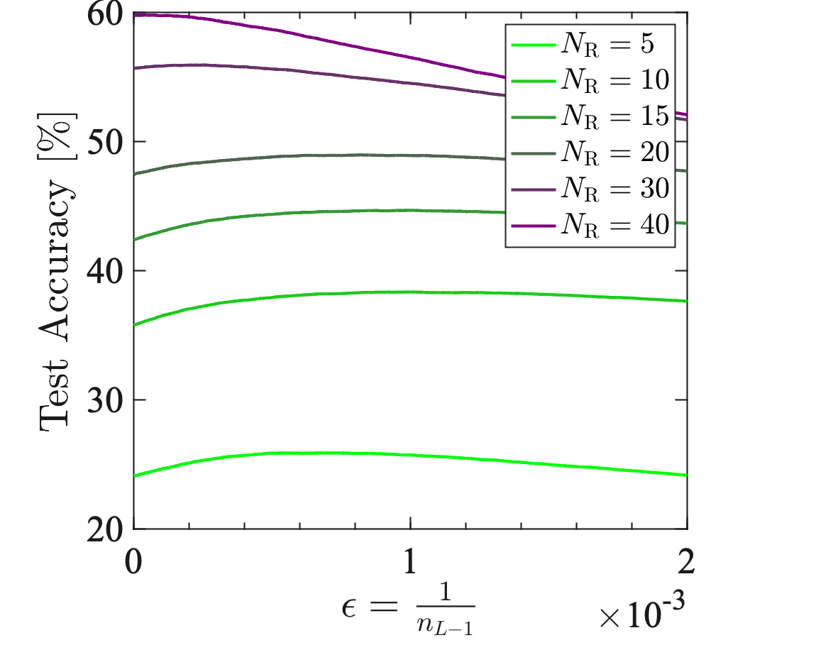
With additional manipulations, this expression can be simplified into the actionable form that is amenable to use in practice [c.f. Equations (NGPM’) and (D) in Appendix D]. It turns out that for deep linear networks the leading finite-width correction vanishes, and the first correction is likely to show up at higher order in asymptotic expansion, which is not carried out in this paper. Here we instead use the multilayer perceptron with the quadratic activation , zero bias variance , and weight variance for illustration, plugging Equations (S30,S31,S32) into Equations (NGPM’) and (D) and varying . Results in Figure 2 indicate the regularization effects of finite widths when the number of training samples, , is small, resulting in peak performance at finite widths. This is in line with expectations that finite widths ameliorate overfitting and that non-Gaussian priors increase the expressivity of neural functions, but additional large-scale extensive experiments would be desirable in the future.
VI Dreams
In this paper, we have developed the perturbative formalism that captures the flow of preactivation distributions from lower to higher layers. The resemblance between our recursive equations and renormalization-group flow equations in high-energy and statistical physics is highly appealing. It would be exciting to investigate the structure of fixed points away from the Gaussian asymptopia Schoenholz et al. (2016) and fully realize the dream articulated in Ref. Mehta and Schwab (2014) – the audacious hypothesis that neural networks wash away microscopic irrelevancies and extract relevant features – beyond their limited example of a mapping between two antiquated techniques.
In addition we have developed the perturbative Bayesian inference scheme universally applicable whenever prior distributions are weakly non-Gaussian, and have applied it to the specific cases of neural networks at finite widths. In light of possible finite-width regularization effects, it would be prudent to revisit the empirical comparison between SGD optimization and Bayesian inference at finite widths Lee et al. (2018); Novak et al. (2019), especially for convolutional neural networks.
Finally, given surging interests in SGD dynamics within the large-width regime Jacot et al. (2018); Chizat et al. (2018); Lee et al. (2019); Cohen et al. (2019); Dyer and Gur-Ari (2019), it would be natural to adapt our formalism for investigating corrections to neural tangent kernels, and even aspire to capture a transition from lazy-learning to feature-learning regimes.
Acknowledgments
The author thanks Yasaman Bahri for the discussion that seeded the idea for this project, Boris L. Hanin for persistently preaching about Gaussian processes, and David J. Schwab for permission to call his example limited with our friendship intact. The author also thanks Ethan S. Dyer, Mario Geiger, Guy Gur-Ari, Eric T. Mintun, Stephen H. Shenker, and Lexing Ying for substantially useful discussions, and Daniel A. Roberts for the quality control of all the jokes and more.
References
- Brown (1828) R. Brown, The Philosophical Magazine 4, 161 (1828).
- Einstein (1905) A. Einstein, Annalen der Physik 322, 549 (1905).
- Weinberg (1995) S. Weinberg, The quantum theory of fields: Volume I: Foundations (Cambridge University Press, 1995).
- Parisi and Zamponi (2010) G. Parisi and F. Zamponi, Reviews of Modern Physics 82, 789 (2010).
- Neal (1996) R. M. Neal, in Bayesian Learning for Neural Networks (Springer, 1996), pp. 29–53.
- Williams (1997) C. K. I. Williams, in Advances in Neural Information Processing Systems (1997), pp. 295–301.
- Lee et al. (2018) J. Lee, Y. Bahri, R. Novak, S. S. Schoenholz, J. Pennington, and J. Sohl-Dickstein, in International Conference on Learning Representations (2018), URL https://openreview.net/forum?id=B1EA-M-0Z.
- Matthews et al. (2018) A. G. d. G. Matthews, M. Rowland, J. Hron, R. E. Turner, and Z. Ghahramani, in International Conference on Learning Representations (2018), URL https://openreview.net/forum?id=H1-nGgWC-.
- Jacot et al. (2018) A. Jacot, F. Gabriel, and C. Hongler, in Advances in Neural Information Processing Systems (2018), pp. 8571–8580.
- Chizat et al. (2018) L. Chizat, E. Oyallon, and F. Bach, arXiv preprint arXiv:1812.07956 (2018).
- Lee et al. (2019) J. Lee, L. Xiao, S. S. Schoenholz, Y. Bahri, J. Sohl-Dickstein, and J. Pennington, arXiv preprint arXiv:1902.06720 (2019).
- Geiger et al. (2019) M. Geiger, S. Spigler, A. Jacot, and M. Wyart, arXiv preprint arXiv:1906.08034 (2019).
- Kadanoff (1966) L. P. Kadanoff, Physics Physique Fizika 2, 263 (1966).
- Wilson (1971) K. G. Wilson, Physical Review B 4, 3174 (1971).
- Weinberg (1996) S. Weinberg, The quantum theory of fields: Volume II: Modern Applications (Cambridge University Press, 1996).
- Goldenfeld (2018) N. Goldenfeld, Lectures on phase transitions and the renormalization group (CRC Press, 2018).
- Mehta and Schwab (2014) P. Mehta and D. J. Schwab, arXiv preprint arXiv:1410.3831 (2014).
- Wick (1950) G.-C. Wick, Physical Review 80, 268 (1950).
- Zee (2010) A. Zee, Quantum field theory in a nutshell (Princeton University Press, 2010).
- Williams and Rasmussen (2006) C. K. I. Williams and C. E. Rasmussen, Gaussian processes for machine learning (MIT Press, 2006).
- Robbins and Monro (1951) H. Robbins and S. Monro, The Annals of Mathematical Statistics 22, 400 (1951).
- MacKay (1995) D. J. C. MacKay, Network: Computation in Neural Systems 6, 469 (1995).
- Cohen et al. (2019) O. Cohen, O. Malka, and Z. Ringel, arXiv preprint arXiv:1906.05301 (2019).
- Dyer and Gur-Ari (2019) E. Dyer and G. Gur-Ari, arXiv preprint arXiv:1909.11304 (2019).
- Antognini (2019) J. M. Antognini, arXiv preprint arXiv:1908.10030 (2019).
- Moshe and Zinn-Justin (2003) M. Moshe and J. Zinn-Justin, Physics Reports 385, 69 (2003).
- Cho and Saul (2009) Y. Cho and L. K. Saul, in Advances in Neural Information Processing Systems (2009), pp. 342–350.
- Liao and Poggio (2017) Q. Liao and T. Poggio, arXiv preprint arXiv:1703.09833 (2017).
- Saxe et al. (2013) A. M. Saxe, J. L. McClelland, and S. Ganguli, arXiv preprint arXiv:1312.6120 (2013).
- Li et al. (2018) Y. Li, T. Ma, and H. Zhang, in Conference On Learning Theory (2018), pp. 2–47.
- Hanin and Rolnick (2018) B. Hanin and D. Rolnick, in Advances in Neural Information Processing Systems (2018), pp. 571–581.
- LeCun et al. (1998) Y. LeCun, L. Bottou, Y. Bengio, and P. Haffner, Proceedings of the IEEE 86, 2278 (1998).
- Schoenholz et al. (2016) S. S. Schoenholz, J. Gilmer, S. Ganguli, and J. Sohl-Dickstein, in International Conference on Learning Representations (2016), URL https://openreview.net/forum?id=H1W1UN9gg.
- Novak et al. (2019) R. Novak, L. Xiao, Y. Bahri, J. Lee, G. Yang, J. Hron, D. A. Abolafia, J. Pennington, and J. Sohl-Dickstein, in International Conference on Learning Representations (2019), URL https://openreview.net/forum?id=B1g30j0qF7.
Appendix A Wick’s tricks
Here is all you need to know in order to follow the calculations in the paper. In the main text, Wick’s contractions are used both for trivially integrating out biases and weights as straightforward applications of Appendix A.1 and for nontrivially integrating out preactivations, with concepts of cumulants reviewed in Appendix A.2 and A.3, culminating in the hack derived in Appendix A.4. The random variables are generically indexed by throughout this Appendix: when applying formulae for biases, ; for weights ; for full preactivations ; for single-neuron preactivations .
A.1 Wick’s contractions
For Gaussian-distributed variables with a kernel , moments
| (S1) |
For any odd such moments identically vanish. For even , Isserlis-Wick’s theorem states that
| (S2) |
where the sum is over all the possible pairings of variables, . In general, there are such pairings. For a proof, see for example Zee (2010). In order to understand and use the theorem, it is instructive to look at a few examples:
| (S3) | |||||
| (S4) |
and
A.2 Connected correlations
Given general (not necessarily Gaussian) random variables, connected correlation functions are defined inductively through
where the sum is over all the possible subdivisions of variables into clusters of sizes as . In order to understand the definition, it is again instructive to look at a few examples. Assuming that all the odd moments vanish,
| (S7) | |||||
Rearranging them in particular yields
If these examples do not suffice, here is yet another example to chew on:
and hence
We emphasize that these are just renderings of the definition (A.2). The power of this definition will be illustrated in the next two subsections.
A.3 Hierarchical clustering
We often encounter situations with the hierarchy
| (S12) |
where is a small perturbative parameter and here again odd moments are assumed to vanish. Often comes with the hierarchical structure is the asymptotic limit where
| (S13) |
with the Gaussian kernel at zero and the leading self-energy correction . Let us also denote the leading four-point vertex
| (S14) |
For instance this hierarchy holds for weakly-coupled field theories – from which we are importing names such as self-energy, vertex, and metric – and, in this paper, such hierarchical structure is inductively shown to hold for prior preactivations with in the regime . Note that, by definition, and are symmetric under and is symmetric under permutations of .777In the main text the connected four-point preactivation correlation functions are symmetric under the permutations of four indices, .
A.4 Combinatorial hack
So far we have reviewed the standard technology of Wick’s contractions, connected correlation functions, and all that. Our objective now is to develop a method to evaluate for random variables obeying the hierarchical-clustering property (S12),888More precisely, we shall inductively use only the weaker proposition that for along with Equations (S13) and (S14). which is the inductive hypothesis made in the main text; by extension, the resulting method (HACK’) lets us perturbatively evaluate for any function that can be obtained as a limit of a sequence of analytic functions.
With the review of connected correlation functions passed us, first note that
| (CLUSTER) | ||||
| (CLUSTER’) | ||||
where in the last equality Wick’s theorem was used backward.
Below, let us use the inverse kernel as a metric to raise indices:
| (S15) | |||||
| (S16) |
Then, in order to simplify the second set of terms in Equation (CLUSTER’) involving self-energy, note that
where the symmetry of was used. Hence, defining
| (OS’) |
we obtain
| (S17) | |||||
| (S18) |
The similar algebraic exercise renders the other term in Equation (CLUSTER’) to be
| (S19) | |||||
| (S20) |
with
| (OV’) |
In summary, for any function of random variables
| (HACK’) |
Appendix B Full condensed proof
In this Appendix, we provide a full inductive proof for one of the main claims in the paper, streamlined in the main text. Namely, we assume at the -th layer that Equations (KS) and (V) hold and that all the higher-point connected preactivation correlation functions are of order – which are trivially true at – and prove the same for the -th layer. We assume the full mastery of Appendix A or, conversely, this section can be used to test the mastery of Wick’s tricks.
First, trivial Wick’s contractions yield
Studiously disentangling cases with different numbers of repetitions in neuron indices , we notice that at order , terms without repetition or with only one repetition contribute, finding
where we used the inductive hierarchical assumption at the -th layer, i.e., its consequence (HACK) and denoted a single-neuron random vector and the Gaussian integral with the core kernel . Plugging in expressions (OS,OV) for operators ,
and
As special cases, we obtain expressions advertised in the main text to be contained in this Appendix:
and
Assembling everything,
In particular,
| (S28) | |||||
| (S29) |
completing our inductive proof. Note that .
Nowhere in our derivation had we assumed anything about the form of activation functions. The only potential exceptions to our formalism are exponentially growing activation functions – which we never see in practice – that would make the Gaussian integrals unintegrable.
Appendix C Bestiary of concrete examples
C.1 Quadratic activation
Let us take multilayer perceptrons with quadratic activation, , and study the distributions of preactivations in the second layer as another illustration of our technology. From the master recursion relations (R1-R3) with the initial condition (R0), Wick’s contractions yield
| (S30) | ||||
| (S31) | ||||
| (S32) |
where . These expressions are used in the main text for the experimental study of finite-width corrections on Bayesian inference.
C.2 Details for single-input cases
The recursive relations simplify drastically for the case of a single input, . Setting for simplicity and dropping index, our recursive equations reduce to
| (S33) | ||||
| (S34) | ||||
| (S35) | ||||
C.2.1 Monomials with single input
For monomial activations, , such as in deep linear networks Saxe et al. (2013) and quadratic activations Li et al. (2018),
| (S36) | ||||
| (S37) | ||||
| (S38) |
In particular the four-point vertex solution is given by
| (S39) |
The factor generalizes the factor for linear and ReLU activations. Following Ref. Hanin and Rolnick (2018), this factor guides us to narrow hidden layers as we pass through nonlinear activations for .
C.2.2 ReLU with single input
ReLU activation, , can also be worked out for a single input through Wick’s contractions, noting that the Gaussian integral is halved, yielding
| (S40) | ||||
| (S41) | ||||
| (S42) |
Setting for simplicity, these equations can be solved, leading to
| (S43) | ||||
| (S44) | ||||
| (S45) |
C.3 More experiments on output distributions
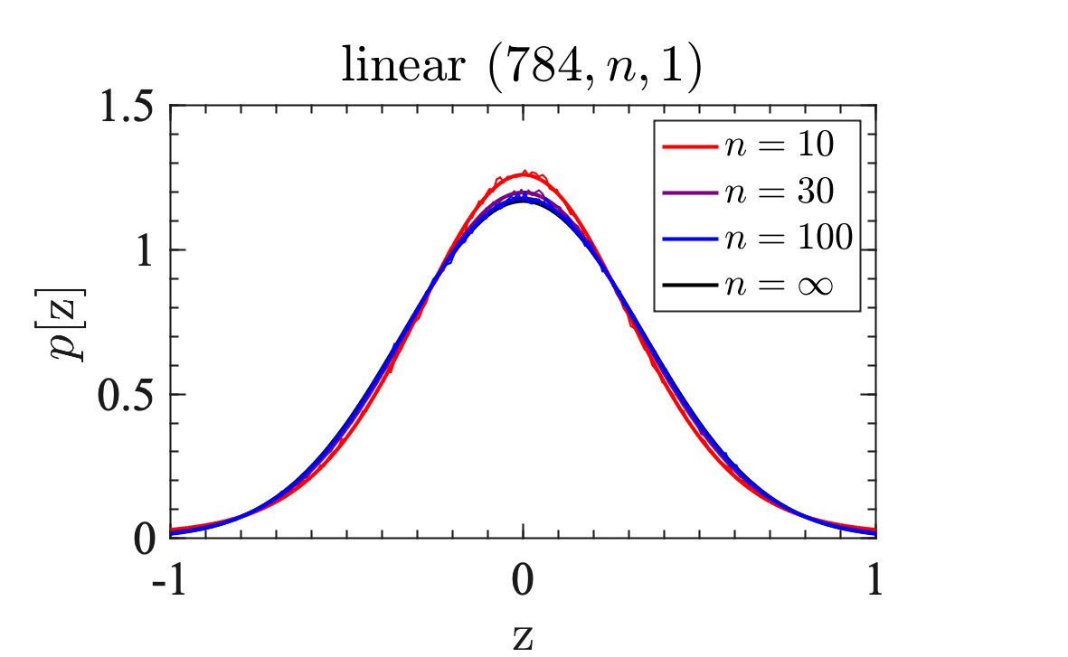
Here is an extended version of experiments in Section IV.3. As in the main text, take a single black-white image of hand-written digits from the MNIST dataset as an -dimensional input, without preprocessing. Set bias variance , weight variance , and use activations (linear) with , (quadratic) with , and (ReLU) with . For all three cases, we consider both depth with widths and depth with widths . As in Figure 1, in Figure S1, for each width-parameter of the hidden layers we record the prior distribution of outputs over instances of Gaussian weights and compare it with the theoretical prediction. Results again corroborate our theory.


Appendix D Finite-width corrections on Bayesian inference
In order to massage Equation (NGPM) into an actionable form, first playing with the metric inversions and defining , the mean prediction becomes
| (S46) | |||
This expression simplifies drastically through the identity
| (S47) |
which can be checked explicitly, recalling . Incidentally, this identity can also be used to prove Equation (GP). Now equipped with this identity, recalling , we notice that and . Similarly
and other components [i.e. with one or both of training components replaced by test components ] vanish. Equation (S46) thus simplifies to
| (S48) | |||
Finally, denoting the matrix inside the parenthesis to be
| (NGPM’) | ||||
and noticing and ,
is the mean prediction. Equations (NGPM’) and (D) with are actionable, i.e., easy to program.