XNOR-Net++: Improved binary neural networks

Abstract

This paper proposes an improved training algorithm for binary neural networks in which both weights and activations are binary numbers. A key but fairly overlooked feature of the current state-of-the-art method of XNOR-Net [Rastegari et al.(2016)Rastegari, Ordonez, Redmon, and Farhadi] is the use of analytically calculated real-valued scaling factors for re-weighting the output of binary convolutions. We argue that analytic calculation of these factors is sub-optimal. Instead, in this work, we make the following contributions: (a) we propose to fuse the activation and weight scaling factors into a single one that is learned discriminatively via backpropagation. (b) More importantly, we explore several ways of constructing the shape of the scale factors while keeping the computational budget fixed. (c) We empirically measure the accuracy of our approximations and show that they are significantly more accurate than the analytically calculated one. (d) We show that our approach significantly outperforms XNOR-Net within the same computational budget when tested on the challenging task of ImageNet classification, offering up to 6% accuracy gain.

1 Introduction

An open problem in deep learning is how to port recent developments into devices other than desktop machines with one or more high-end GPUs, such as the devices that billions of users use in their everyday life and work like cars, smart-phones, tablets, TVs etc. The straightforward approach to solving this problem is to train models that are both smaller and faster. One of the prominent methods for achieving both goals is through training binary networks, especially when both activations and network weights are binary [Courbariaux et al.(2015)Courbariaux, Bengio, and David, Courbariaux et al.(2016)Courbariaux, Hubara, Soudry, El-Yaniv, and Bengio, Rastegari et al.(2016)Rastegari, Ordonez, Redmon, and Farhadi]. In this case, the binary convolution can be efficiently implemented using the XNOR gate, resulting in model compression ratio of $\sim 32\times$ and speed-up of $\sim 58\times$ on CPU [Rastegari et al.(2016)Rastegari, Ordonez, Redmon, and Farhadi]. As there is no such thing as a free lunch, these impressive figures come at the cost of reduced accuracy. For example, there is $\sim 18\%$ drop in top-1 accuracy between a real-valued ResNet-18 and its binary counterpart on ImageNet [Rastegari et al.(2016)Rastegari, Ordonez, Redmon, and Farhadi]. The main aim of this work is to try to bridge this gap by training more powerful binary networks.

The key observation made in the seminal work of [Rastegari et al.(2016)Rastegari, Ordonez, Redmon, and Farhadi] is that one can compensate to some extent for the error caused by the binary approximation by re-scaling the output of the binary convolution using real-valued scale factors. This maintains all the advantages of binary convolutions by adding a negligible number of parameters and complexity. Our key observation in this work is regarding how these scaling factors are computed. While the authors of [Rastegari et al.(2016)Rastegari, Ordonez, Redmon, and Farhadi] used an analytic approximation for each layer, we argue that this is sub-optimal for learning the task in hand, and propose to learn these factors discriminatively via backpropagation. This allows the network to optimize the scaling factors with respect to the loss function of the task in hand rather than trying to reduce the approximation error induced by the binarization.

In particular, we make the following contributions:

• We propose to fuse the activation and weight scaling factors into a single one that is learned discriminatively via backpropagation. Further, we propose several ways to construct the shape of these scale factors keeping the complexity at test time fixed. Our constructs increase the expressivity of the scaling factors that are now statistically learned both spatially and channel-wise (Section 4.1).

• We empirically measure the accuracy of our approximations and show that they are significantly more accurate than the analytically calculated one (Section 4.2).

• We show that our improved training of binary networks is agnostic to network architecture used by applying it to both shallow and deep residual networks.

• Exhaustive experiments conducted on the challenging ImageNet dataset show that our method offers an improvement of more than 6% in absolute terms over the state-of-the-art (Section 5).

2 Related work

This section offers a brief overview of the relevant work on designing deep learning methods suitable for running under tight computational constraints. In order to achieve this, in the recent years, a series of different techniques have been proposed such as: network pruning [Lin et al.(2017a)Lin, Rao, Lu, and Zhou, Han et al.(2015)Han, Mao, and Dally, Molchanov et al.(2016)Molchanov, Tyree, Karras, Aila, and Kautz], which consists of removing the least important weights/activations, conditional computation [Bengio et al.(2015)Bengio, Bacon, Pineau, and Precup], low rank approximations [Kim et al.(2015)Kim, Park, Yoo, Choi, Yang, and Shin, Lebedev et al.(2014)Lebedev, Ganin, Rakhuba, Oseledets, and Lempitsky, Kossaifi et al.(2019)Kossaifi, Bulat, Tzimiropoulos, and Pantic], which decompose the weights and enforce a low rank constraint on them, designing of efficient architectures [He et al.(2016a)He, Zhang, Ren, and Sun, He et al.(2016b)He, Zhang, Ren, and Sun] and network quantization [Zhou et al.(2016)Zhou, Wu, Ni, Zhou, Wen, and Zou, Lin et al.(2015)Lin, Talathi, and Annapureddy]. A detailed review of all of these different techniques goes beyond the scope of this paper, so herein we will focus on presenting the closest to our work: designing efficient architectures and network quantization, focusing, more specifically, on network binarization [Courbariaux et al.(2016)Courbariaux, Hubara, Soudry, El-Yaniv, and Bengio, Rastegari et al.(2016)Rastegari, Ordonez, Redmon, and Farhadi, Bulat and Tzimiropoulos(2017)].

2.1 Efficient neural networks

With the increase in popularity of mobile devices a large body of work on designing efficient convolutional networks has emerged. From an architectural standpoint such methods take either a holistic approach (i.e. improving the overall structure) or local, by improving the convolutional block or the convolution operation itself.

Local optimization. Since the groundbreaking work of Krizhevsky et al. [Krizhevsky et al.(2012)Krizhevsky, Sutskever, and Hinton] that introduced the AlexNet architecture, subsequent work attempted to improve the overall accuracy while reducing the computational demand. In VGG [Simonyan and Zisserman(2014)], the large convolutional filters previously used in AlexNet (up to $11\times 11$) were replaced with a series of smaller $3\times 3$ filters that had an equivalent receptive field size (e.g. 2 convolutional layers with $3\times 3$ filters are equivalent with one that has $5\times 5$ filters). This idea is further explored in the numerous versions of the inception block [Szegedy et al.(2015)Szegedy, Liu, Jia, Sermanet, Reed, Anguelov, Erhan, Vanhoucke, and Rabinovich, Szegedy et al.(2016)Szegedy, Vanhoucke, Ioffe, Shlens, and Wojna, Szegedy et al.(2017)Szegedy, Ioffe, Vanhoucke, and Alemi] where one of the proposed changes was to decompose some of the convolutional layers that have a $3\times 3$ kernel into two consecutive layers with $1\times 3$ and $3\times 1$ kernels, respectively. In [He et al.(2016a)He, Zhang, Ren, and Sun], He et al. introduce the so-called “bottleneck” block that reduces the number of channels processed by large filters (i.e. $3\times 3$) using 2 convolutional layers with a $1\times 1$ kernel that project the features into a lower dimensional space and back. This idea is further explored in [Xie et al.(2016)Xie, Girshick, Dollár, Tu, and He] where the convolutional layers with $3\times 3$ filters are decomposed into a series of independent smaller layers with the help of grouped convolutions. Similar ideas are explored in MobileNet [Howard et al.(2017)Howard, Zhu, Chen, Kalenichenko, Wang, Weyand, Andreetto, and Adam] and MobileNet-v2 [Sandler et al.(2018)Sandler, Howard, Zhu, Zhmoginov, and Chen] that use point-wise grouped convolutions and inverted residual modules, respectively. Chen et al. [Chen et al.(2019)Chen, Fang, Xu, Yan, Kalantidis, Rohrbach, Yan, and Feng] propose to factorize the feature maps of a convolutional network by their frequencies, introducing an adapted convolution operation that stores and processes feature maps that vary spatially “slower” at a lower spatial resolution reducing the overall computation cost and memory footprint.

Holistic optimization. Most of the recent architectures build upon the landmark work of He et al. [He et al.(2016a)He, Zhang, Ren, and Sun] that proposed the so-called Residual networks. Dense-Net [Huang et al.(2016)Huang, Liu, Weinberger, and van der Maaten], for example, adds a connection from a given layer inside a macro-module to every other layer. In [Redmon et al.(2016)Redmon, Divvala, Girshick, and Farhadi] and its improved versions [Redmon and Farhadi(2017), Redmon and Farhadi(2018)], the authors introduce the “You Only Look Once”(YOLO) architecture which designs a new framework for object detection with a specially optimized topology for the network backbone that allows for real-time or near real-time performance on a modern high-end GPU.

Note, that in this work, we do not attempt to improve the network architecture itself and instead explore our novel approach in the context of both shallow (AlexNet [Krizhevsky et al.(2012)Krizhevsky, Sutskever, and Hinton]) and deep residual networks (ResNets [He et al.(2016a)He, Zhang, Ren, and Sun, He et al.(2016b)He, Zhang, Ren, and Sun]) showing that our method is orthogonal and complementary to methods that propose better network topologies.

2.2 Network binarization

With the rise of in-hardware support for low-precision operations, recently, network quantization has emerged as a natural way of improving the efficiency of CNNs by aligning them with the underlining hardware implementations. Of particular interest is the extreme case of quantization - network binarization, where the features and the weights of a neural network are quantized to two states, typically $\{\pm 1\}$.

While initially binarization was thought to be unfeasible due to the extreme quantization errors introduced, recent work suggests otherwise [Courbariaux et al.(2014)Courbariaux, Bengio, and David, Courbariaux et al.(2015)Courbariaux, Bengio, and David, Courbariaux et al.(2016)Courbariaux, Hubara, Soudry, El-Yaniv, and Bengio, Rastegari et al.(2016)Rastegari, Ordonez, Redmon, and Farhadi]. However, despite of the recent effort, training fully binary networks remains notoriously difficult. It is important to note that among the methods that make use of binarization, some of them binarize the weights [Courbariaux et al.(2015)Courbariaux, Bengio, and David, Faraone et al.(2018)Faraone, Fraser, Blott, and Leong, Tang et al.(2017)Tang, Hua, and Wang] while keeping the input signal either real or quantized to n-bits, and some of them additionally binarize the signal too [Rastegari et al.(2016)Rastegari, Ordonez, Redmon, and Farhadi, Courbariaux et al.(2016)Courbariaux, Hubara, Soudry, El-Yaniv, and Bengio, Bulat and Tzimiropoulos(2017), Bulat and Tzimiropoulos(2018)]. Because the input features dominate the overall memory consumption (especially for large batch sizes), an effective binarization approach should ideally binarize both weights and features. Not only does this reduce the memory footprint, but also allows the replacement of all the multiplications used in a convolutional layer with bitwise operations. In this work, we study and attempt to improve this particular case of interest.

The method of [Zhou et al.(2016)Zhou, Wu, Ni, Zhou, Wen, and Zou] Zhou et al. allocates a different number of bits per each network component based on their sensitivity to numerical inaccuracies. As such, the method proposes to use 1 bit for the weights, 2 for the activations and 6 for the gradients. [Wang et al.(2018)Wang, Hu, Zhang, Zhang, Liu, and Cheng] introduces a n-bit quantization method ($n\geq 2$), in which a low-bit code is firstly composed and then a transformation function is learned. In [Faraone et al.(2018)Faraone, Fraser, Blott, and Leong], the authors quantize the weights using 1 to 2 bits and the features using 2 to 8 bits, by learning a symmetric codebook for each particular weight subgroup.

The foundations of the fully binarized networks were laid out in [Courbariaux et al.(2014)Courbariaux, Bengio, and David] and the follow-up works of [Courbariaux et al.(2015)Courbariaux, Bengio, and David, Courbariaux et al.(2016)Courbariaux, Hubara, Soudry, El-Yaniv, and Bengio]. To reduce the quantization error and improve their expressivity, in [Rastegari et al.(2016)Rastegari, Ordonez, Redmon, and Farhadi], the authors propose to use two real-valued scaling factors, one for the weights and one for activations. The proposed XNOR-Net [Rastegari et al.(2016)Rastegari, Ordonez, Redmon, and Farhadi] is the first method to report good results on a large-scale dataset (ImageNet). In this work, we propose to fuse the activation and weight scaling factors into a single one which is learned discriminatively instead of computing them analytically as in [Rastegari et al.(2016)Rastegari, Ordonez, Redmon, and Farhadi]. We also motivate and explore various ways for constructing the shape of the factors.

Bulat&Tzimiropoulos [Bulat and Tzimiropoulos(2017)] propose a novel residual block specifically designed for binary networks for localization tasks, addressing the binarization problem from a network topology standpoint. In [Zhou et al.(2018)Zhou, Yao, Wang, and Chen], Zhou et al. proposes a loss-aware binarization method that jointly regularizes the approximation error and the task loss. Motivated by the fact that for large batch sizes most of the memory is taken by activations, the method of [Mishra et al.(2017)Mishra, Cook, Nurvitadhi, and Marr] proposes to increase the network width (represented by the number of channels of a given convolutional layer). Similarly, the work of [Lin et al.(2017b)Lin, Zhao, and Pan] introduces the ABC-Net that uses up to 5 parallel binary convolutional layers to approximate a real one. While this increases the network accuracy, it does so at a high cost as the resulting network is up to 5$\times$ slower. In contrast, we improve the overall accuracy of fully binarized networks within the same computational budget.

3 Background

This section reviews the binarization process proposed in [Courbariaux et al.(2015)Courbariaux, Bengio, and David] alongside XNOR-Net, its improved version from [Rastegari et al.(2016)Rastegari, Ordonez, Redmon, and Farhadi], which still represents the state-of-the-art method for training binary networks.

For a given layer $L$ of a CNN architecture we denote with $\mathcal{W}\in\mathbb{R}^{o\times c\times w\times h}$ and $\mathcal{I}\in\mathbb{R}^{c\times w_{in}\times h_{in}}$ its weights and input features, where $o$ represents the number of output channels, $c$ the number of input channels and ($w,h$) the width and height of the convolutional kernel. Moreover, $w_{in}\geq w$ and $h_{in}\geq h$ represent the spatial dimensions of $\mathcal{I}$. Following [Courbariaux et al.(2015)Courbariaux, Bengio, and David], the binarization is done by taking the sign of the weights and input features, where

$$\text{sign}(x)=\begin{cases}-1,&\mbox{if }x\leq 0\\ 1,&\mbox{if }x>0\end{cases}.$$ (1)

Because binarization is a highly destructive process in which large quantization errors are induced, the achieved accuracy, especially on challenging datasets (such as Imagenet) is low. To alleviate this, Rastegari et al. [Rastegari et al.(2016)Rastegari, Ordonez, Redmon, and Farhadi] introduce two analytically calculated real-valued scaling factors, one for the weights and one for the input features, which are used to re-weight the output of a binary convolution as follows:

$$\mathcal{I}\ast\mathcal{W}\approx\left(\text{sign}(\mathcal{I})\stackMath\mathbin{\stackinset{c}{0ex}{c}{0ex}{\ast}{\bigcirc}}\text{sign}(\mathcal{W})\right)\odot\mathcal{K}\mathbf{\alpha},$$ (2)

where $\odot$ denotes the element-wise multiplication, $\ast$ the real-valued convolution operation and $\stackMath\mathbin{\stackinset{c}{0ex}{c}{0ex}{\ast}{\bigcirc}}$ its binary counterpart (implemented using bitwise operations), $\mathbf{\alpha}_{i}=\frac{\left\lVert\mathcal{W}_{i,\,\boldsymbol{:}\,,\,\boldsymbol{:}\,,\,\boldsymbol{:}\,}\right\rVert_{\ell 1}}{n},~{}i=\{1,2,\cdots,o\}$, $n=c\times w\times h$ is the weight scaling factor, and $\mathcal{K}$ the activation scaling factor. $\mathcal{K}$ is efficiently computed by convolving $\mathcal{A}=\frac{\sum\lVert I_{i,\,\boldsymbol{:}\,,\,\boldsymbol{:}\,}\rVert}{c}$ with a 2D filter $k\in\mathbb{R}^{w\times h}$, where $\forall{ij}~{}k_{ij}=\frac{1}{w\times h}$. Note, that as the calculation of $\mathcal{K}$ is relatively expensive due to the fact that it is recomputed at each forward pass, it is common to drop it at the expense of a slight drop in accuracy [Rastegari et al.(2016)Rastegari, Ordonez, Redmon, and Farhadi, Bulat and Tzimiropoulos(2017)]. In contrast, in this work, we fuse $\mathbf{\alpha}$ and $\mathcal{K}$ into a single factor that is learned via backpropagation. In the process, we motivate and explore various ways of forming the shape of this factor.

4 Method

In this section, we firstly present, in Sub-section 4.1, our proposed improved binarization technique, coined XNOR-Net++, that increases the representational power of binary networks by describing novel ways to construct scaling factors for the binary convolutional layers. Next, Sub-sections 4.2 and 4.3 analyze empirically the performance of our method and, the speed-up and memory savings offered.

4.1 XNOR-Net++

As mentioned earlier (see Section 4.2), directly binarizing the weights and the input features of a given layer using the sign function is known to induce high quantization errors. To alleviate this, in [Rastegari et al.(2016)Rastegari, Ordonez, Redmon, and Farhadi], one of the key elements that allowed the training of more accurate binary networks on challenging datasets was the introduction of the scaling factors $\mathbf{\alpha}$ and $\mathcal{K}$ for the weight and features, respectively (see also Section 3). While the analytical solution provided in [Rastegari et al.(2016)Rastegari, Ordonez, Redmon, and Farhadi] works well, in general, it fails to take in consideration the overall task at hand and has limited flexibility since obtaining a good minimum is directly tight with the distribution of the binary weights. Moreover, computing the scaling factor with respect to the features is relatively expensive and needs to be done for every new input.

To alleviate this, in this work, we propose to fuse the activation and weight scaling factors into a single one, denoted as $\Gamma$, that is learned discriminatively via backpropagation. This allows us to capture a statistical representation of our data, facilitates the learning process and even has the advantage that at test time the analytic calculation of these factors is not required, thus reducing the number of real-valued operations. In particular, we propose to re-formulate Eq. (2) as:

$$\mathcal{I}\ast\mathcal{W}\approx\left(\text{sign}(\mathcal{I})\stackMath\mathbin{\stackinset{c}{0ex}{c}{0ex}{\ast}{\bigcirc}}\text{sign}(\mathcal{W})\right)\odot\Gamma$$ (3)

This new formulation allows us to explore various ways of constructing the shape of $\Gamma$ during training. Specifically, we propose to construct $\Gamma$ in the following 4 ways:

Case 1:

$$\Gamma=\mathbf{\alpha},~{}~{}\mathbf{\alpha}\in\mathbb{R}^{o\times 1\times 1}$$ (4)

Case 2:

$$\Gamma=\mathbf{\alpha},~{}~{}\mathbf{\alpha}\in\mathbb{R}^{o\times h_{out}\times w_{out}}$$ (5)

Case 3:

$$\Gamma=\mathbf{\alpha}\otimes\mathbf{\beta},~{}~{}\mathbf{\alpha}\in\mathbb{R}^{o},\mathbf{\beta}\in\mathbb{R}^{h_{out}\times w_{out}}$$ (6)

Case 4:

$$\Gamma=\mathbf{\alpha}\otimes\mathbf{\beta}\otimes\mathbf{\gamma},~{}~{}\mathbf{\alpha}\in\mathbb{R}^{o},\mathbf{\beta}\in\mathbb{R}^{h_{out}},\mathbf{\gamma}\in\mathbb{R}^{w_{out}}$$ (7)

Case 1: The first straightforward approach is to simply learn one scaling factor per each input channel, similarly to what a Batch Normalization layer would do. As Tables 1 and 2 show learning this alone instead of computing it analytically is already significantly better than the analytically calculated factors proposed in [Rastegari et al.(2016)Rastegari, Ordonez, Redmon, and Farhadi].

Case 2: While Case 1 works reasonably well, it fails to capture the information en-capsuled over the spatial dimensions. To address this, in Eq. (5), we propose to learn a dense scaling, one value for each output pixel, which as Table 1 shows, performs 0.6% better than the previous version.

Case 3: While Case 2 performs 0.6% better than the previous version, it is relatively large in size and harder to optimize often leading to some sort of overfitting. As such, in Eq. (6), we propose to decompose this dense scaling into two terms combined using an outer product. As Eq. (6) shows, $\mathbf{\alpha}$ learns the statistics over the output channel dimension while $\mathbf{\beta}$ over the spatial dimensions. With a reduced number of parameters, when compared to our previous version, this further boosts the performance by 0.6%.

Case 4: Upon analyzing $\mathbf{\beta}$ in Case 3, we noticed that it is low rank and as such further compressions are possible. This leads us to the final version shown in Eq. (7), where we learn a rank-1 factor for each mode (channels, height, weight). This further reduces the number of parameters making their number negligible when compared with the overall number of weights present inside a layer and improves the performance by a further 0.4%.

Note, that in all cases, during testing, the factors are merged together into a single one and a single element-wise product takes place (see also Section 4.3).

Method	shapes	Top-1 acc.	Top-5 acc.
baseline [Rastegari et al.(2016)Rastegari, Ordonez, Redmon, and Farhadi]	-	51.2%	73.2%
Case 1: $\mathbf{\alpha}$	$\mathbf{\alpha}\in\mathbb{R}^{o\times 1\times 1}$	55.5%	78.5%
Case 2: $\mathbf{\alpha}$	$\mathbf{\alpha}\in\mathbb{R}^{o\times h_{out}\times w_{out}}$	56.1%	79.0%
Case 3: $\mathbf{\alpha\otimes\beta}$	$\mathbf{\alpha}\in\mathbb{R}^{o},\mathbf{\beta}\in\mathbb{R}^{w_{out}\times h_{out}}$	56.7%	79.5%
Case 4: $\mathbf{\alpha\otimes\beta\otimes\gamma}$	$\mathbf{\alpha}\in\mathbb{R}^{o},\mathbf{\beta}\in\mathbb{R}^{w_{out}}$ $\mathbf{\gamma}\in\mathbb{R}^{h_{out}}$	57.1%	79.9%

Table 1: Top-1 and Top-5 classification accuracy using a binarized ResNet-18 on Imagenet for various ways of constructing the scaling factor. $\mathbf{\alpha},\mathbf{\beta},\mathbf{\gamma}$ are statistically learned via backpropagation. Note that, at test time, all of them can be merged into a single factor, and a single element-wise multiplication is required.

4.2 Empirical performance analysis

In Section 5, we showcased the advantages of learning a single scaling factor $\Gamma$ discriminatively and explored various ways to construct it for further improving the achieved accuracy for the task of ImageNet classification. Herein, we reach similar conclusions by analyzing the quantization loss, and more specifically, by showing that, for a given real-valued convolutional layer, our method can approximate its output with a binary convolution with higher fidelity.

For our experiments, we created a convolutional layer with $\mathcal{W}\in\mathbb{R}^{64\times 64\times 3\times 3}$ and $\mathcal{I}\in\mathbb{R}^{64\times 16\times 16}$ both initialized from a normal distribution. We then tried to compute an equivalent binary layer having as target to minimize the reconstruction error between its output and the one of the real-valued layer. As shown in [Rastegari et al.(2016)Rastegari, Ordonez, Redmon, and Farhadi], the optimal solution for the binary weights is given by $\text{sign}(\mathcal{W})$. Although [Rastegari et al.(2016)Rastegari, Ordonez, Redmon, and Farhadi] does develop an analytic solution for the weights, this solution is only an approximation. Hence, for the needs of our experiment, we fixed the binary weights as $\text{sign}(\mathcal{W})$ and then trained the scaling factors for the cases proposed in section 4.1. The layer is trained until convergence using Adam [Kingma and Ba(2014)] (SGD and RMSProp gave similar results). We then repeated the process 100 times, for different $\mathcal{W}$ and $\mathcal{I}$. The L1 distance between the output of the real convolution and that of the binary one is shown in Table 2. Notice that our methods consistently outperforms [Rastegari et al.(2016)Rastegari, Ordonez, Redmon, and Farhadi] by a large margin.

Method	shapes	L1 distance
Direct binarization [Courbariaux et al.(2016)Courbariaux, Hubara, Soudry, El-Yaniv, and Bengio]	-	$6.36\pm 0.04$
Baseline XNOR [Rastegari et al.(2016)Rastegari, Ordonez, Redmon, and Farhadi]	-	$0.095\pm 0.002$
Case 1: $\mathbf{\alpha}$	$\mathbf{\alpha}\in\mathbb{R}^{o\times 1\times 1}$	$0.038\pm 0.001$
Case 3: $\mathbf{\alpha\otimes\beta}$	$\mathbf{\alpha}\in\mathbb{R}^{o},\mathbf{\beta}\in\mathbb{R}^{w_{out}\times h_{out}}$	$0.037\pm 0.001$
Case 4: $\mathbf{\alpha\otimes\beta\otimes\gamma}$	$\mathbf{\alpha}\in\mathbb{R}^{o},\mathbf{\beta}\in\mathbb{R}^{w_{out}}$ $\mathbf{\gamma}\in\mathbb{R}^{h_{out}}$	$\mathbf{0.035\pm 0.001}$

Table 2: L1 distance between the output of a real-valued convolutional layer and its binary counterpart using different methods for learning the scale factors. In all cases, the binary weights are fixed as $\text{sign}(\mathcal{W})$. Note that, in XNOR-Net, the scale factors are not learned but analytically calculated.

4.3 Efficiency analysis

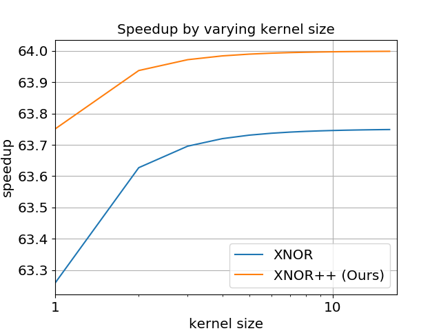
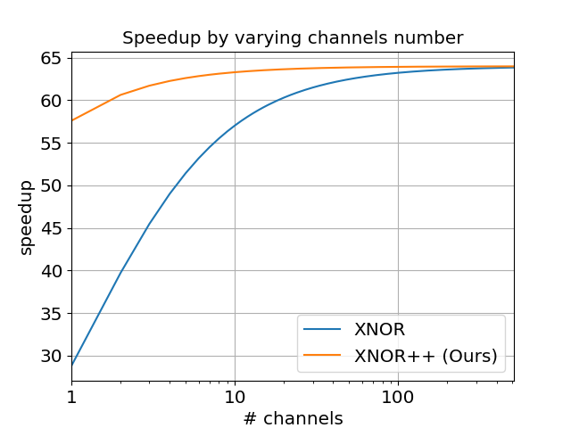
Figure 1: Theoretical speed-up offered by our method and [Rastegari et al.(2016)Rastegari, Ordonez, Redmon, and Farhadi].

An important aspect of binary convolutions are the speed-ups offered. Assuming an implementation with no algorithmic optimizations, the total number of operations for a given convolutional layer is $N=c\times w\times h\times w_{out}\times h_{out}\times o$. Given the usage of bit-packing and an SIMD approach, a modern CPU can execute 64$\times$ more binary operations per clock than multiplications. Since the XNOR-Net [Rastegari et al.(2016)Rastegari, Ordonez, Redmon, and Farhadi] method computes an independent scale for the weights and the features, in addition to $N$ XNOR ops, the binary layer will require $2\times c\times h_{out}\times w_{out}$ multiplications and $c\times h_{out}\times w_{out}\times h\times w$ additions, making the overall theoretical speed-up approx. equal to:

$$S_{XNOR}=\frac{64\times w\times h\times o}{w\times h\times o+2+h\times w}.$$ (8)

In contrast, since our method fuses the scaling factors, it only requires $c\times w_{out}\times h_{out}$ additional floating point operations:

$$S_{OURS}=\frac{64\times w\times h\times o}{w\times h\times o+1}.$$ (9)

Notice that the speed-up is independent of the input feature resolution and does not include the memory access cost. Assuming a layer with 256 output channels and a kernel size of $3\times 3$ (one of the most common layers found in a Resnet architecture [He et al.(2016a)He, Zhang, Ren, and Sun]), $S_{XNOR}\approx 63.69\times$ while $S_{OURS}\approx 63.98\times$. In terms of storage, similarly to BNN and XNOR-Net, our method can take advantage of bit-packing offering a space saving of $\approx 64\times$.

5 Results

In this section, we describe the experimental setting used in our work and compare our method against other state-of-the-art binary networks. We show that our approach largely outperforms the current top performing methods by more than 6% on ImageNet classification.

5.1 Experimental setup

This section describes the experimental setup of our paper going through the dataset and networks used and providing details regarding the training process.

5.1.1 Network architecture

Herein, we describe the topology of the two networks used: AlexNet [Krizhevsky et al.(2012)Krizhevsky, Sutskever, and Hinton] and ResNet-18 [He et al.(2016a)He, Zhang, Ren, and Sun] alongside their modifications, if any.

ResNet-18. We preserved the overall network architecture (i.e. 18 layers distributed over 4 macro-blocks; except for the first and last layer all of them are grouped in pairs of 2 inside a basic block [He et al.(2016a)He, Zhang, Ren, and Sun]). We note that we followed [Rastegari et al.(2016)Rastegari, Ordonez, Redmon, and Farhadi] and used the basic block version with pre-activation [He et al.(2016b)He, Zhang, Ren, and Sun] moving the activation function after the convolution and adding a sign function before it.

AlexNet. In line with previous works [Rastegari et al.(2016)Rastegari, Ordonez, Redmon, and Farhadi, Courbariaux et al.(2016)Courbariaux, Hubara, Soudry, El-Yaniv, and Bengio], we removed the local normalization operation and added a batch normalization [Ioffe and Szegedy(2015)] layer followed by a sign activation before each convolutional layer. Additionally, we kept the dropout on both fully connected layers setting its value to 0.5.

As in [Rastegari et al.(2016)Rastegari, Ordonez, Redmon, and Farhadi], the first and last layers for both networks were kept real.

5.1.2 Datasets

We trained and evaluated our models on ImageNet [Deng et al.(2009)Deng, Dong, Socher, Li, Li, and Fei-Fei]. ImageNet is a large-scale image recognition dataset containing 1.2M training and 50,000 validation samples distributed over 1000 non-overlapping classes.

5.1.3 Training

For training both ResNet-18 [He et al.(2016a)He, Zhang, Ren, and Sun] and AlexNet [Krizhevsky et al.(2012)Krizhevsky, Sutskever, and Hinton] we follow the common practices used for training binary nets [Rastegari et al.(2016)Rastegari, Ordonez, Redmon, and Farhadi]: we resized the input images to $256\times 256$px and then randomly cropped them during training to $224\times 224$px for ResNet and $227\times 227$px for AlexNet, while during testing we center-cropped them to the corresponding sizes. For both models, the initial learning rate was set to $10^{-3}$ and the weight decay to $10^{-5}$. The learning rate was dropped during training every 25 epochs by a factor of 10. The entire training process runs for 80 epochs. Similarly to [Rastegari et al.(2016)Rastegari, Ordonez, Redmon, and Farhadi], we used a batch size of 400 for AlexNet and 256 for ResNet. The weights are initialized as in [He et al.(2016a)He, Zhang, Ren, and Sun].

All of our models were trained using Adam [Kingma and Ba(2014)]. They are implemented in Pytorch [Paszke et al.(2017)Paszke, Gross, Chintala, Chanan, Yang, DeVito, Lin, Desmaison, Antiga, and Lerer].

5.2 Comparison with state-of-the-art

In this section, we compare the performance of our approach against those of other state-of-the-art methods that binarize both the weights and the features within the same computational budget. We note that most of prior work only binarize the weights and use either full precision or n-bits quantized activations and as such cannot take advantage of the large speed-ups offered by full binary convolutions. We also note that to allow for a fair comparison, we compare only against methods that use the same number of weights: to achieve high accuracy, ABC-Net increases the network size $25\times$, while their version which has the same number of parameters as ours (i.e. for M=N=1 using a ResNet-18, where M and N represent the expansion rates for the features and weights respectively) achieves a top-1 accuracy of 42.2% only (vs 57.1% achieved by our methods).

Our results are summarized in Table 3: when using ResNet-18, our method significantly outperforms the state-of-the-art by about 6% in terms of absolute error using both Top-1 and Top-5 metrics. For AlexNet, we observe that the improvement was not as great. In general, we found that AlexNet was much harder to train and prone to overfitting.

Method	AlexNet		ResNet-18
	Top-1 accuracy	Top-5 accuracy	Top-1 accuracy	Top-5 accuracy
BNN [Courbariaux et al.(2016)Courbariaux, Hubara, Soudry, El-Yaniv, and Bengio]	41.8%	67.1%	42.2%	69.2%
XNOR-Net [Rastegari et al.(2016)Rastegari, Ordonez, Redmon, and Farhadi]	44.2%	69.2%	51.2%	73.2%
Bethge et al. [Bethge et al.(2018)Bethge, Bornstein, Loy, Yang, and Meinel]	-	-	54.4%	77.5%
Ours	46.9%	71.0%	57.1%	79.9%
Real valued [Krizhevsky et al.(2012)Krizhevsky, Sutskever, and Hinton]	56.6%	80.2%	69.3%	89.2%

Table 3: Top-1 and Top-5 classification accuracy using binarized AlexNet and ResNet-18 architectures on the validation set of Imagenet.

6 Conclusion

We revisited the calculation of scale factors used to re-weight the output of binary convolutions by proposing to learn them discriminatively via backpropagation. We also explored different shapes for these factors. We showed large improvements of up to $6\%$ on ImageNet classification using ResNet-18.

References

- [Bengio et al.(2015)Bengio, Bacon, Pineau, and Precup] Emmanuel Bengio, Pierre-Luc Bacon, Joelle Pineau, and Doina Precup. Conditional computation in neural networks for faster models. arXiv preprint arXiv:1511.06297, 2015.
- [Bethge et al.(2018)Bethge, Bornstein, Loy, Yang, and Meinel] Joseph Bethge, Marvin Bornstein, Adrian Loy, Haojin Yang, and Christoph Meinel. Training competitive binary neural networks from scratch. arXiv preprint arXiv:1812.01965, 2018.
- [Bulat and Tzimiropoulos(2017)] Adrian Bulat and Georgios Tzimiropoulos. Binarized convolutional landmark localizers for human pose estimation and face alignment with limited resources. In ICCV, 2017.
- [Bulat and Tzimiropoulos(2018)] Adrian Bulat and Yorgos Tzimiropoulos. Hierarchical binary cnns for landmark localization with limited resources. IEEE Transactions on Pattern Analysis and Machine Intelligence, 2018.
- [Chen et al.(2019)Chen, Fang, Xu, Yan, Kalantidis, Rohrbach, Yan, and Feng] Yunpeng Chen, Haoqi Fang, Bing Xu, Zhicheng Yan, Yannis Kalantidis, Marcus Rohrbach, Shuicheng Yan, and Jiashi Feng. Drop an octave: Reducing spatial redundancy in convolutional neural networks with octave convolution. arXiv preprint arXiv:1904.05049, 2019.
- [Courbariaux et al.(2014)Courbariaux, Bengio, and David] Matthieu Courbariaux, Yoshua Bengio, and Jean-Pierre David. Training deep neural networks with low precision multiplications. arXiv, 2014.
- [Courbariaux et al.(2015)Courbariaux, Bengio, and David] Matthieu Courbariaux, Yoshua Bengio, and Jean-Pierre David. Binaryconnect: Training deep neural networks with binary weights during propagations. In NIPS, 2015.
- [Courbariaux et al.(2016)Courbariaux, Hubara, Soudry, El-Yaniv, and Bengio] Matthieu Courbariaux, Itay Hubara, Daniel Soudry, Ran El-Yaniv, and Yoshua Bengio. Binarized neural networks: Training deep neural networks with weights and activations constrained to+ 1 or-1. arXiv, 2016.
- [Deng et al.(2009)Deng, Dong, Socher, Li, Li, and Fei-Fei] Jia Deng, Wei Dong, Richard Socher, Li-Jia Li, Kai Li, and Li Fei-Fei. Imagenet: A large-scale hierarchical image database. In CVPR, 2009.
- [Faraone et al.(2018)Faraone, Fraser, Blott, and Leong] Julian Faraone, Nicholas Fraser, Michaela Blott, and Philip HW Leong. Syq: Learning symmetric quantization for efficient deep neural networks. In Proceedings of the IEEE Conference on Computer Vision and Pattern Recognition, pages 4300–4309, 2018.
- [Han et al.(2015)Han, Mao, and Dally] Song Han, Huizi Mao, and William J Dally. Deep compression: Compressing deep neural networks with pruning, trained quantization and huffman coding. arXiv preprint arXiv:1510.00149, 2015.
- [He et al.(2016a)He, Zhang, Ren, and Sun] Kaiming He, Xiangyu Zhang, Shaoqing Ren, and Jian Sun. Deep residual learning for image recognition. In CVPR, 2016a.
- [He et al.(2016b)He, Zhang, Ren, and Sun] Kaiming He, Xiangyu Zhang, Shaoqing Ren, and Jian Sun. Identity mappings in deep residual networks. In ECCV, 2016b.
- [Howard et al.(2017)Howard, Zhu, Chen, Kalenichenko, Wang, Weyand, Andreetto, and Adam] Andrew G Howard, Menglong Zhu, Bo Chen, Dmitry Kalenichenko, Weijun Wang, Tobias Weyand, Marco Andreetto, and Hartwig Adam. Mobilenets: Efficient convolutional neural networks for mobile vision applications. arXiv preprint arXiv:1704.04861, 2017.
- [Huang et al.(2016)Huang, Liu, Weinberger, and van der Maaten] Gao Huang, Zhuang Liu, Kilian Q Weinberger, and Laurens van der Maaten. Densely connected convolutional networks. arXiv, 2016.
- [Ioffe and Szegedy(2015)] Sergey Ioffe and Christian Szegedy. Batch normalization: Accelerating deep network training by reducing internal covariate shift. arXiv, 2015.
- [Kim et al.(2015)Kim, Park, Yoo, Choi, Yang, and Shin] Yong-Deok Kim, Eunhyeok Park, Sungjoo Yoo, Taelim Choi, Lu Yang, and Dongjun Shin. Compression of deep convolutional neural networks for fast and low power mobile applications. arXiv preprint arXiv:1511.06530, 2015.
- [Kingma and Ba(2014)] Diederik P Kingma and Jimmy Ba. Adam: A method for stochastic optimization. arXiv preprint arXiv:1412.6980, 2014.
- [Kossaifi et al.(2019)Kossaifi, Bulat, Tzimiropoulos, and Pantic] Jean Kossaifi, Adrian Bulat, Georgios Tzimiropoulos, and Maja Pantic. T-net: Parametrizing fully convolutional nets with a single high-order tensor. In Proceedings of the IEEE Conference on Computer Vision and Pattern Recognition, pages 7822–7831, 2019.
- [Krizhevsky et al.(2012)Krizhevsky, Sutskever, and Hinton] Alex Krizhevsky, Ilya Sutskever, and Geoffrey E Hinton. Imagenet classification with deep convolutional neural networks. In NIPS, 2012.
- [Lebedev et al.(2014)Lebedev, Ganin, Rakhuba, Oseledets, and Lempitsky] Vadim Lebedev, Yaroslav Ganin, Maksim Rakhuba, Ivan Oseledets, and Victor Lempitsky. Speeding-up convolutional neural networks using fine-tuned cp-decomposition. arXiv preprint arXiv:1412.6553, 2014.
- [Lin et al.(2015)Lin, Talathi, and Annapureddy] Darryl D Lin, Sachin S Talathi, and V Sreekanth Annapureddy. Fixed point quantization of deep convolutional networks. arXiv, 2015.
- [Lin et al.(2017a)Lin, Rao, Lu, and Zhou] Ji Lin, Yongming Rao, Jiwen Lu, and Jie Zhou. Runtime neural pruning. In Advances in Neural Information Processing Systems, pages 2181–2191, 2017a.
- [Lin et al.(2017b)Lin, Zhao, and Pan] Xiaofan Lin, Cong Zhao, and Wei Pan. Towards accurate binary convolutional neural network. In Advances in Neural Information Processing Systems, pages 345–353, 2017b.
- [Mishra et al.(2017)Mishra, Cook, Nurvitadhi, and Marr] Asit Mishra, Jeffrey J Cook, Eriko Nurvitadhi, and Debbie Marr. Wrpn: Training and inference using wide reduced-precision networks. arXiv preprint arXiv:1704.03079, 2017.
- [Molchanov et al.(2016)Molchanov, Tyree, Karras, Aila, and Kautz] Pavlo Molchanov, Stephen Tyree, Tero Karras, Timo Aila, and Jan Kautz. Pruning convolutional neural networks for resource efficient transfer learning. arXiv preprint arXiv:1611.06440, 3, 2016.
- [Paszke et al.(2017)Paszke, Gross, Chintala, Chanan, Yang, DeVito, Lin, Desmaison, Antiga, and Lerer] Adam Paszke, Sam Gross, Soumith Chintala, Gregory Chanan, Edward Yang, Zachary DeVito, Zeming Lin, Alban Desmaison, Luca Antiga, and Adam Lerer. Automatic differentiation in pytorch. 2017.
- [Rastegari et al.(2016)Rastegari, Ordonez, Redmon, and Farhadi] Mohammad Rastegari, Vicente Ordonez, Joseph Redmon, and Ali Farhadi. Xnor-net: Imagenet classification using binary convolutional neural networks. In ECCV, 2016.
- [Redmon and Farhadi(2017)] Joseph Redmon and Ali Farhadi. Yolo9000: better, faster, stronger. In Proceedings of the IEEE conference on computer vision and pattern recognition, pages 7263–7271, 2017.
- [Redmon and Farhadi(2018)] Joseph Redmon and Ali Farhadi. Yolov3: An incremental improvement. arXiv preprint arXiv:1804.02767, 2018.
- [Redmon et al.(2016)Redmon, Divvala, Girshick, and Farhadi] Joseph Redmon, Santosh Divvala, Ross Girshick, and Ali Farhadi. You only look once: Unified, real-time object detection. In Proceedings of the IEEE conference on computer vision and pattern recognition, pages 779–788, 2016.
- [Sandler et al.(2018)Sandler, Howard, Zhu, Zhmoginov, and Chen] Mark Sandler, Andrew Howard, Menglong Zhu, Andrey Zhmoginov, and Liang-Chieh Chen. Mobilenetv2: Inverted residuals and linear bottlenecks. In Proceedings of the IEEE Conference on Computer Vision and Pattern Recognition, pages 4510–4520, 2018.
- [Simonyan and Zisserman(2014)] Karen Simonyan and Andrew Zisserman. Very deep convolutional networks for large-scale image recognition. arXiv, 2014.
- [Szegedy et al.(2015)Szegedy, Liu, Jia, Sermanet, Reed, Anguelov, Erhan, Vanhoucke, and Rabinovich] Christian Szegedy, Wei Liu, Yangqing Jia, Pierre Sermanet, Scott Reed, Dragomir Anguelov, Dumitru Erhan, Vincent Vanhoucke, and Andrew Rabinovich. Going deeper with convolutions. In CVPR, 2015.
- [Szegedy et al.(2016)Szegedy, Vanhoucke, Ioffe, Shlens, and Wojna] Christian Szegedy, Vincent Vanhoucke, Sergey Ioffe, Jon Shlens, and Zbigniew Wojna. Rethinking the inception architecture for computer vision. In Proceedings of the IEEE conference on computer vision and pattern recognition, pages 2818–2826, 2016.
- [Szegedy et al.(2017)Szegedy, Ioffe, Vanhoucke, and Alemi] Christian Szegedy, Sergey Ioffe, Vincent Vanhoucke, and Alexander A Alemi. Inception-v4, inception-resnet and the impact of residual connections on learning. In AAAI, 2017.
- [Tang et al.(2017)Tang, Hua, and Wang] Wei Tang, Gang Hua, and Liang Wang. How to train a compact binary neural network with high accuracy? In Thirty-First AAAI Conference on Artificial Intelligence, 2017.
- [Wang et al.(2018)Wang, Hu, Zhang, Zhang, Liu, and Cheng] Peisong Wang, Qinghao Hu, Yifan Zhang, Chunjie Zhang, Yang Liu, and Jian Cheng. Two-step quantization for low-bit neural networks. In Proceedings of the IEEE Conference on Computer Vision and Pattern Recognition, pages 4376–4384, 2018.
- [Xie et al.(2016)Xie, Girshick, Dollár, Tu, and He] Saining Xie, Ross Girshick, Piotr Dollár, Zhuowen Tu, and Kaiming He. Aggregated residual transformations for deep neural networks. arXiv, 2016.
- [Zhou et al.(2018)Zhou, Yao, Wang, and Chen] Aojun Zhou, Anbang Yao, Kuan Wang, and Yurong Chen. Explicit loss-error-aware quantization for low-bit deep neural networks. In CVPR, 2018.
- [Zhou et al.(2016)Zhou, Wu, Ni, Zhou, Wen, and Zou] Shuchang Zhou, Yuxin Wu, Zekun Ni, Xinyu Zhou, He Wen, and Yuheng Zou. Dorefa-net: Training low bitwidth convolutional neural networks with low bitwidth gradients. arXiv, 2016.