Thermodynamics of AdS₅ black holes: holographic QCD and Stückelberg model

Abstract

We explore the thermodynamics of AdS₅ black holes in two models: i) an improved holographic QCD model with a simple dilaton potential, and ii) the Stückelberg model in 5D. In the former case, by applying techniques of singular perturbation theory, we obtain a resummation of the naive expansion at high temperatures, providing a good fit to the lattice data for the trace anomaly. In the latter, we find a solution of the equations of motion by considering an expansion in the conformal dimension of the current associated to the gauge field.

1 Introduction

The gauge/gravity duality is a powerful tool to study the properties of gauge theories, and in particular of QCD, in their strongly coupled regime. Using this duality, the thermodynamics of a field theory can be obtained from the classical computation of the thermodynamics of black holes in the gravity dual. The entropy of a black hole can be computed from the famous Bekenstein-Hawking entropy formula [1, 2, 3, 4, 5]. In conformal AdS₅ the entropy scales like $S_{\textrm{Black Hole}}\propto r_{h}^{3}\propto T^{3}$; however, in order to have a reliable extension of this duality to SU($\text{N}_{c}$) Yang-Mills theory, the first task is to control the breaking of conformal invariance. Conformal transformations are broken by quantum corrections due to the necessary regularization of the UV divergences, yielding the so-called trace anomaly [6, 7]

$$\langle T^{\mu}_{\mu}\rangle=-\varepsilon+3p=-\frac{\beta(g)}{2g^{3}}\langle(F_{\mu\nu}^{a})^{2}\rangle\,,$$ (1)

where $T^{\mu\nu}$ is the energy-momentum tensor, $\varepsilon$ is the energy density, $p$ is the pressure and $\beta$ is the beta function. We will explore the application of techniques of singular perturbation theory to get a better control of the high temperature expansion of the thermodynamic quantities.

On the other hand, theories with a massive gauge field in the bulk of AdS₅ have been proposed as holographic duals of QCD with dynamical gauge fields. The relation of the Stückelberg field in holography to the axial anomaly has been first pointed out in Ref. [8]. Recent applications of the Stückelberg mechanism include the computation of anomalous effective actions [9], anomalous transport and their renormalization properties [10, 11], AdS/QCD [12] and beyond the Standard Model scenarios [13]. In the last part of this work we will study the thermodynamics of the Stückelberg model in 5D as well as the consistency of the entropy formula in this model.

2 The holographic QCD model

The bottom-up approach is based on the building of a gravity dual of QCD, including the main properties of this theory. We introduce in this section the model and study the solutions.

2.1 The model

One of the most successful holographic models of QCD within the bottom-up scenario is the 5D Einstein-dilaton model, with the Euclidean action [2]

$$\begin{split}S&=\frac{1}{2\kappa^{2}}\int d\rho\,d^{4}x\sqrt{G}\Bigl{(}-R+G^{\mu\nu}\partial_{\mu}\Phi\partial_{\nu}\Phi+2V(\Phi)\Bigr{)}+S_{{\mathrm{GH}}}\,,\end{split}$$ (2)

where $\kappa^{2}=1/(2M^{3})$ is the 5D Newton constant with $M$ the Planck mass, and $\Phi$ is a scalar field to be identified with the Yang-Mills coupling through $g^{2}=e^{\gamma\Phi}$. The boundary term $S_{{\mathrm{GH}}}$ is the usual Gibbons-Hawking contribution built up from the extrinsic curvature. The introduction of a scalar field breaks conformal invariance, and the form of the scalar potential $V(\Phi)$ is usually phenomenologically adjusted to describe some observables of QCD. We can introduce the superpotential, whose relation with the scalar potential is $V(\Phi)=\frac{1}{2}W^{\prime}(\Phi)^{2}-\frac{2}{3}W(\Phi)^{2}$. In this work we will consider the simple form of the superpotential

$$W(\Phi)=\ell^{-1}(3+v_{0}e^{\gamma\Phi})\,,$$ (3)

where $\ell$ is the radius of the asymptotically AdS₅ background. The combination $\gamma^{2}v_{0}/2\equiv b_{0}$ can be taken from the one-loop $\beta$-function of a pure SU($\text{N}_{c}$) gauge theory, i.e.

$$\beta(g):=\mu\frac{dg}{d\mu}=-b_{0}g^{3}=-\frac{11\,\text{N}_{c}}{3(4\pi)^{2}}g^{3}\,.$$ (4)

2.2 Equations of motion

We are interested in the study of finite temperature solutions of the Einstein-scalar gravity model corresponding to a black hole. In Fefferman-Graham coordinates the metric is

$$ds^{2}=G_{\mu\nu}dx^{\mu}dx^{\nu}=\frac{\ell^{2}}{4\rho^{2}}d\rho^{2}+\frac{\ell^{2}}{\rho}g_{\tau\tau}(\rho)d\tau^{2}+\frac{\ell^{2}}{\rho}g_{xx}(\rho)d{\vec{x}}^{2}\,.$$ (5)

The asymptotic expansions for the metric and the dilaton field in holographic QCD models have been studied in details in these coordinates [14]. This metric has a regular horizon at $\rho=\rho_{h}$, i.e. $g_{\tau\tau}(\rho_{h})=g_{\tau\tau}^{\prime}(\rho_{h})=0$, and the temperature and entropy density of the black hole are given by

$$T=\frac{1}{2\pi}\sqrt{2\rho_{h}g_{\tau\tau}^{\prime\prime}(\rho_{h})}\,,\qquad s=\frac{2\pi}{\kappa^{2}}\left(\frac{\ell^{2}}{\rho_{h}}g_{xx}(\rho_{h})\right)^{3/2}\,.$$ (6)

Using this metric, the equation for the scalar field, which is a second order differential equation, can be decoupled by an additional differentiation. Then it can be converted in autonomous by making the change of variables, $(\rho,\Phi)\to(\Phi,u(\Phi))$, where $u(\Phi)\equiv\rho\,\Phi^{\prime}(\rho)$, leading to 

$$u^{\prime\prime}(\Phi)=\frac{\bigl{(}u^{\prime}(\Phi)\bigr{)}^{2}}{u(\Phi)}-\frac{3\ell^{2}V^{\prime}(\Phi)}{4u(\Phi)^{2}}u^{\prime}(\Phi)+\frac{\ell^{4}\bigl{(}V^{\prime}(\Phi)\bigr{)}^{2}}{16u(\Phi)^{3}}+\frac{\ell^{2}\bigl{(}8V(\Phi)+3V^{\prime\prime}(\Phi)\bigr{)}}{12u(\Phi)}\,.$$ (7)

At zero temperature, when $g_{xx}=g_{\tau\tau}$, the solution corresponds to a domain wall configuration, $u_{0}(\Phi)=\frac{\ell}{2}W^{\prime}(\Phi)=\tfrac{\gamma v_{0}}{2}e^{\gamma\Phi}$, and it is given by

$$e^{\gamma\Phi(\rho)}=\frac{2}{\gamma^{2}v_{0}\,\log\left(\rho_{0}/\rho\right)}\,,\qquad g_{xx}(\Phi)=g_{\tau\tau}(\Phi)=g_{(0)}\cdot e^{-2\Phi/(3\gamma)}\,.$$ (8)

Using $g^{2}=e^{\gamma\Phi}$ and Eq. (4), it turns out that the radial coordinate $\rho^{-1/2}$ can be interpreted as the renormalization group (RG) scale, and $\rho_{0}^{-1/2}\equiv\Lambda_{{\mathrm{QCD}}}$ is an integration constant corresponding to the location of the Landau pole of QCD. The other integration constant $g_{(0)}$ is arbitrary.

2.3 Asymptotically AdS black hole solutions from resummation

We now consider a black hole solution specified by the horizon data $(\rho_{h},\Phi_{h})$. Local analysis of the equations of motion shows that, in order to have a regular horizon at $\Phi=\Phi_{h}$, it is necessary that $\lim_{\Phi\to\Phi_{h}}\bigl{(}u(\Phi)g^{\prime}_{xx}(\Phi)-g_{xx}(\Phi)\bigr{)}=0$, which fixes the first term of the power series solution

$$u(\Phi)=\sum_{n=0}^{\infty}a_{n}(\Phi_{h})(\Phi_{h}-\Phi)^{n+1/2}\,,$$ (9)

and similar expressions for $g_{xx}(\Phi)$ and $g_{\tau\tau}(\Phi)$. We will study the analytical solution in the regime $\nu\equiv\gamma v_{0}e^{\gamma\Phi_{h}}\ll 1$ for any $\gamma>0$ by using a boundary-layer analysis. In this regime the leading part of each coefficient of the series (9) behaves as $a_{n}(\Phi_{h})\propto\nu^{-n+1/2}$. This suggests to consider an expansion of the form $u^{\mathrm{in}}(\Phi)=\sum_{n=1}^{\infty}\nu^{n}U_{n}((\Phi_{h}-\Phi)/\nu)$ which is valid in the region of boundary-layer near the horizon, where the inner variable, $\Psi\equiv(\Phi_{h}-\Phi)/\nu$, is $O(1)$. The first order of this expansion reads $u^{\mathrm{in}}(\Phi)=\frac{\nu}{2}\sqrt{1-e^{-4\Psi}}+O(\nu^{2})$. For the regime outside the boundary layer we tried a solution of the form $u^{\mathrm{out}}(\Phi)=\sum_{n=1}^{\infty}\nu^{n}u_{n}(\Phi_{h}-\Phi)$, and the corresponding substitution in Eq. (7) leads to $u^{\mathrm{out}}(\Phi)=\frac{\nu}{2}e^{\gamma(\Phi-\Phi_{h})}$ to all orders in $\nu$, so that the outer solution has the same form as the zero temperature solution. Thus the asymptotic matching produces a uniform approximation valid for $(-\infty,\Phi_{h})$ given by

$$u^{\mathrm{unif}}(\Phi)=\frac{v_{0}\gamma}{2}e^{\gamma\Phi}+u^{\mathrm{in}}(\Phi)-\frac{v_{0}\gamma}{2}e^{\gamma\Phi_{h}}+O(\nu^{2})\,,$$ (10)

so that $|u(\Phi)-u^{\mathrm{unif}}(\Phi)|=O(\nu^{2})$. The last term in Eq. (10) is the common limit of the inner and outer approximation in the matching region, $\nu\ll\Phi_{h}-\Phi\ll 1$.

From the knowledge of the lowest orders of $u^{\mathrm{in}}(\Phi)$, it is possible to get in closed form the lowest orders in $\nu$ for the inner solutions of the metric, $g_{ij}^{\mathrm{in}}(\Phi)=\sum_{n}\nu^{n}g_{(n)ij}(\Psi)$, while the outer solution reduces to the zero temperature result given by Eq. (8). Finally, the asymptotic matching of the outer solution with the inner expansion determines the horizon quantities

$$g_{xx}(\Phi_{h}) =2g_{(0)}e^{-2\Phi_{h}/(3\gamma)}\left(1-\frac{\nu\,\log 2}{3\gamma}+O(\nu^{2})\right)\,,$$ (11)

$$g_{\tau\tau}^{\prime}(\Phi_{h}) =-\frac{8g_{(0)}e^{-2\Phi_{h}/(3\gamma)}}{\nu}\left(1+\frac{\nu}{12\gamma}(4+3\gamma^{2}-4\log 2)+O(\nu^{2})\right)\,.$$ (12)

Note that the second derivative in Eq. (6) is written as $g_{\tau\tau}^{\prime\prime}(\rho_{h})=\rho_{h}^{-2}\lim_{\Phi\to\Phi_{h}}\bigl{(}u(\Phi)u^{\prime}(\Phi)g_{\tau\tau}^{\prime}(\Phi)\bigr{)}$, so that these quantities are directly related to the temperature and entropy of the black hole.

3 Thermodynamics of holographic QCD

Using the previous results, we can apply the holographic prescription [16] for the derivation of the trace anomaly of the Yang-Mills theory (see e.g. Ref. [2] for full details on the procedure).

3.1 Trace Anomaly

The perturbative running of the coupling constant in Yang-Mills theory induces a deformation in the action which may be written as

$$\delta S=\delta\left(\frac{1}{2g^{2}}\right)\int d{{}^{4}}x\,\Tr F^{2}=\int d{{}^{4}}x\left(\frac{\gamma}{2}e^{-\gamma\Phi}\delta\Phi\right)\left(-\Tr F^{2}\right)\,.$$ (13)

This gives rise to the trace anomaly of the stress tensor

$$T^{\mu}_{\mu}=-\frac{\beta(g)}{g^{3}}\Tr F^{2}=b_{0}\Tr F^{2}\,.$$ (14)

To apply the holographic prescription we can assume that the boundary value of the combination $\frac{\gamma}{2b_{0}}e^{-\gamma\Phi(\rho)}\delta\Phi(\rho)$ plays the role of a source that couples to the dual operator $\mathcal{O}=-b_{0}\Tr F^{2}$. The one-point function $\langle\mathcal{O}\rangle$ is therefore proportional to the gluon condensate.

With the zero temperature solution $\Phi_{0}(\rho)$ given by Eq. (8) and $\gamma^{2}v_{0}/2=b_{0}$, one can prove that a change in the scale $\delta\rho_{0}$, induces a change in the scalar field $\delta\Phi$ of the form $\frac{\gamma}{2b_{0}}e^{-\gamma\Phi_{0}}\delta\Phi=-\frac{\delta\rho_{0}}{2\rho_{0}}$. Then, according with Eq. (13), the derivative of the free energy density $w$ with respect to $\log\rho_{0}$ must be proportional to the gluon condensate, leading to

$$2\rho_{0}\frac{\partial w}{\partial\rho_{0}}=b_{0}\langle\Tr F^{2}\rangle\qquad\textrm{where}\qquad S=\frac{V_{3}}{T}\,w\,.$$ (15)

3.2 First law of thermodynamics

We then assume that the free energy density is a function of the source $\rho_{0}$ and the temperature $T$, whose variation is $dw=-s\,dT-\langle\mathcal{O}\rangle d\rho_{0}/(2\rho_{0})$. This assumption requires the condition for integrability $2\rho_{0}\partial s/\partial\rho_{0}=\partial\langle\mathcal{O}\rangle/\partial T$, which has been checked in Ref. [15] by using holographic renormalization techniques. Since there is no conserved charge, the Euler identity adopts the form $w=\varepsilon-Ts$. Then, it follows that the first law of thermodynamics is

$$d\varepsilon=T\,ds-\langle\mathcal{O}\rangle\frac{d\rho_{0}}{2\rho_{0}}\,.$$ (16)

At this point one can observe that there is a similarity to the thermodynamic identities of elastic bodies, where the work done by an applied stress $\tau_{ij}$ is given by $dW=-V_{3}\tau_{ij}\,d\eta_{ij}$, being $\eta_{ij}$ the strain deformation and $V_{3}$ the volume, see e.g. Refs. [17, 18]. This means that the source $\sim\log\sqrt{\rho_{0}}$ plays the role of the deformation, while the condensate $\langle\mathcal{O}\rangle$ is the analogous of the stress tensor. There is no need to interpret the source as any kind of chemical potential [19, 20], and this analogy with the thermodynamics of deformation seems more suitable.

3.3 Equation of state when $\nu\ll 1$

Using dimensional analysis one finds that a compact way of writing the pressure is

$$p(T,\rho_{0})=-w=aT^{4}+aT^{4}\,{\mathcal{N}}(T^{2}\rho_{0})\,,$$ (17)

where $a$ is a constant and ${\mathcal{N}}(x)$ is a function to be determined. We may now compute the pressure from the information about the horizon encoded in Eqs. (11) and (12), which determine the temperature and entropy density when $T\sqrt{\rho_{h}}\gg 1$ and $\Phi_{h}\to-\infty$. When using the relation $\rho_{h}\simeq 2\rho_{0}\exp\left(-\frac{2}{\gamma^{2}v_{0}}e^{-\gamma\Phi_{h}}\right)$, one obtains for the entropy density 

$$\frac{s}{T^{3}}=T^{-3}\frac{\partial p}{\partial T}=4a+4a\,{\mathcal{N}}(T^{2}\rho_{0})+2a\,T^{2}\rho_{0}\,{\mathcal{N}}^{\prime}(T^{2}\rho_{0})\,,$$ (18)

with $a=\ell^{3}\pi^{4}/(2\kappa^{2})$ and ${\mathcal{N}}(x)=-\frac{3}{\mathcal{W}\left(3v_{0}^{-1}(g_{(0)}^{-1}\pi^{2}x)^{3\gamma^{2}/2}\right)}+O(\mathcal{W}^{-2})$, where $\mathcal{W}(z)$ denotes the principal branch of the Lambert $\mathcal{W}$-function. The trace of the thermal stress tensor can be obtained from the relation, $\varepsilon+p=Ts=T\partial_{T}p$, as

$$\varepsilon-3p=-b_{0}\langle\Tr F^{2}\rangle=\frac{\ell^{3}\pi^{4}\gamma^{2}T^{4}}{2\kappa^{2}}{\mathcal{N}}(T^{2}\rho_{0})^{2}+\ldots\,.$$ (19)

The asymptotic behavior $\mathcal{W}(z)\sim\log z$ as $z\to\infty$ is consistent with the logarithmic behavior of the trace anomaly at high temperature. Note that in the opposite limit, $\mathcal{W}(z)\approx z$ as $z\to 0$, the model seems to predict the existence of power corrections in temperature. Although these corrections are desirable, as we will see below they don’t play any phenomenological role within this model. However, it is remarkable that the resummation performed above leads to such a result. Finally, we display in the left panel of Fig. 1 the entropy density (normalized to $T^{3}$) as a function of the inverse of temperature. Note that this is a multivalued function with two regimes corresponding to big (upper branch) and small (lower branch) black holes.

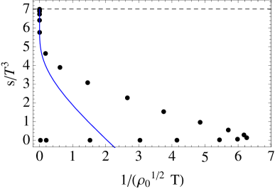
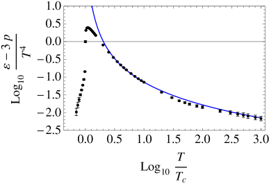
Figure 1: Left panel: $s/T^{3}$ as a function of $(\rho_{0}^{1/2}T)^{-1}$. We display as dots the result from a numerical computation of the equations of motion, while the solid (blue) line corresponds to the analytical result of Eq. (18). The horizontal dashed lines correspond to the Stefan-Boltzmann limit. We have used $\text{N}_{c}=3$ and $\gamma=\sqrt{2/3}$. Right panel: $(\varepsilon-3p)/T^{4}$ as a function of $T$. The dots correspond to the lattice data for gluodynamics from [21] with $\text{N}_{c}=3$. We show as a solid (blue) line the analytical result from Eq. (19) with the values of the parameters given in Sec. 3.4.

3.4 Phenomenological consequences for QCD

We can now compare the results of the model by considering $\gamma$ and $\rho_{0}$ as free parameters, with the lattice data of the equation of state of gluodynamics in SU(3). The best fit to the lattice data of the trace anomaly of Ref. [21] for temperatures $3T_{c}\leq T\leq 1000T_{c}$ leads to $\gamma=2.375(19)$ and $\rho_{0}T_{c}^{2}/g_{(0)}=0.0555(10)$, with $\chi^{2}/\textrm{dof}=0.088$. The result for the trace anomaly is displayed in the right panel of Fig. 1. We conclude that the model leads to an accurate description of the lattice data in the whole regime $3\leq T/T_{c}$. For temperatures closer to $T_{c}$, it has been discussed in the literature that a good description of the lattice data requires the existence of power corrections in $T^{2}$, see e.g. Refs. [22, 23]. However, from this analysis it seems to be that the model does not lead to power corrections in this regime. In either case, we cannot exclude that power corrections could become relevant after considering the effects of RG flows connecting two fixed points, a study already outlined in Ref. [15], or in a sophisticated version of the model.

4 The Stückelberg model

In the last part of this work we will study the thermodynamics of the Stückelberg model in 5D. This model is an extension of the Einstein-Maxwell theory including a massive gauge field.

4.1 The model

The Stückelberg model in 5D is defined by the Euclidean action

$$S=\int dzd^{4}x\sqrt{G}\bigg{[}\frac{1}{2\kappa^{2}}\left(R+\frac{12}{\ell^{2}}\right)-\frac{1}{4g_{5}^{2}}F_{\mu\nu}F^{\mu\nu}-\frac{1}{2g_{5}^{2}}G^{\mu\nu}(\partial_{\mu}\Phi-mA_{\mu})(\partial_{\nu}\Phi-mA_{\nu})\bigg{]}+S_{{\mathrm{GH}}}\,,$$ (20)

where $A_{\mu}$ is a U($1$) gauge field with mass $m$. The mass of the gauge field is related to the conformal dimension $\tilde{\Delta}$ of the U($1$) current operator $J^{\mu}$ dual to the gauge potential as $m^{2}\ell^{2}=(\Delta-3)(\Delta-1)$ with $3\leq\Delta<4$, where for convenience we have defined $\Delta:=3-\tilde{\Delta}$. Let us consider for the moment the metric in conformal coordinates

$$ds^{2}=\frac{\ell^{2}}{z^{2}}\left[dz^{2}+g_{ij}dx^{i}dx^{j}\right]\,,$$ (21)

which is asymptotically AdS₅ near the boundary, $z\to 0$. The behavior of the time component of the gauge field in this regime is

$$A_{\tau}(z)=A_{(0)\tau}\left(\frac{z}{\ell}\right)^{3-\Delta}+{\cal O}^{\tau}_{A}\left(\frac{z}{\ell}\right)^{\Delta-1}+\cdots\,,$$ (22)

where $A_{(0)\tau}$ corresponds to a deformation of the conformal field theory (CFT), with energy scale $\Lambda=1/\ell$, i.e.

$$\int d^{4}x\,A_{(0)\tau}{\mathcal{J}}=\int d^{4}x\,\Lambda^{3-\Delta}A_{(0)\tau}{\cal O}^{\tau}_{A}\,.$$ (23)

In this expression ${\cal O}^{\tau}_{A}\equiv{\mathcal{J}}\Lambda^{\Delta-3}$ is a condensate of dimension $\Delta$, while $A_{(0)\tau}$ plays the role of a chemical potential.

4.2 Black hole solution

The equations of motion of the model follow from the variation of the action with respect to scalar and gauge fields, and the metric. Since we are interested in black hole solutions, we will consider the following ansatz

$$ds^{2}=\frac{r^{2}f(r)}{\ell^{2}}d\tau^{2}+\frac{\ell^{2}}{r^{2}g(r)}dr^{2}+\frac{r^{2}}{\ell^{2}}d{\vec{x}}^{2}\,,\qquad A(r)=j(r)d\tau\,,\qquad\Phi(r)\;=\;\textrm{const}\,,$$ (24)

where we have used $r=\ell^{2}/z$, and seek for perturbative solutions to first order in $\Delta-3$. The leading order solution, $\Delta=3$, corresponds to the well-known result in the Einstein-Maxwell theory in 5D, which reads

$$f_{0}(r)=g_{0}(r)\;=\;\left(1-\frac{r_{h}^{2}}{r^{2}}\right)\left(1+\frac{r_{h}^{2}}{r^{2}}-\frac{q^{2}}{r_{h}^{2}r^{4}}\right)\,,\qquad j_{0}(r)=A_{(0)\tau}\left(1-\frac{r_{h}^{2}}{r^{2}}\right)\,,$$ (25)

where the charge associated to the U($1$) symmetry is $q=\sqrt{\frac{2}{3}}\frac{A_{(0)\tau}\ell r_{h}^{2}\kappa}{g_{5}}$, and the temperature of the black hole is $T_{0}=\frac{r_{h}}{\pi\ell^{2}}\left(1-\frac{q^{2}}{2r_{h}^{6}}\right)$. We use the parametrization

$$f(r)=f_{0}(r)\left(1+F(r)\right)\,,\qquad g(r)=f_{0}(r)\left(1+F(r)+G(r)\right)\,,\qquad j(r)=j_{0}(r)+J(r)\,,$$ (26)

where $F,\;G,\;J$ are corrections of $O(\Delta-3)$. By plugging these functions into the equations of motion, one gets two first order differential equations for $F$ and $G$, and one second order differential equation for $J$. Then there are four integration constants that can be fixed from: i) asymptotically AdS₅ of the solution, i.e. $f(r)\to 1$ as $r\to\infty$; ii) regularity of $F(r)$ at the horizon; iii) vanishing of $A_{\tau}(r)$ at the horizon, or equivalently $J(r_{h})=0$; and finally iV) the behavior of $A_{\tau}$ near the boundary must be $A_{\tau}(r)\sim A_{(0)\tau}\left(\frac{r}{\ell}\right)^{\Delta-3}$, cf. Eq. (22). These conditions fix the constants and determine the temperature as a function of $r_{h}$ and $A_{(0)\tau}$, so that

$$T(r_{h},A_{(0)\tau})=T_{0}\left(1+\frac{\delta T}{T_{0}}\right)\quad\textrm{where}\qquad\frac{\delta T}{T_{0}}=F(r_{h})+\frac{1}{2}G(r_{h})\,.$$ (27)

The explicit expressions for $f(r)$, $g(r)$ and $j(r)$ are too complicated to be shown here, but we will provide below the explicit results for the thermodynamical quantities which simplify a lot.

4.3 Renormalization

In order to get the renormalized action, we need to add appropriate counterterms to cancel the divergences of the action at the boundary. In Fefferman-Graham coordinates the metric becomes as in Eq. (5), while the gauge field is $A=A_{\tau}(\rho)d\tau$ with $\rho=z^{2}$. From $g(r)$ one can obtain the asymptotic series giving $r$ in terms of $z$. The expansion near the boundary turns out to be

$$r=\frac{\ell^{2}}{z}+a_{1}z+a_{3}z^{3}+a_{5}z^{5}+b_{5}z^{5}\log z+\cdots\,,\qquad z\to 0\,,$$ (28)

with the lowest order coefficient given by $a_{1}=-q^{2}m^{2}/(8r_{h}^{4})$. This series expansion yields explicit expressions for the metric components $g_{xx}(\rho)$ and $g_{\tau\tau}(\rho)$ near the boundary. After a straightforward computation, one can write the bulk contribution of the action as a total derivative, and then identify the counterterm needed to cancel the divergences. The result is

$$S_{{\mathrm{ct}}}=\frac{1}{2\kappa^{2}}\int d^{4}x\sqrt{h}\,\frac{6}{\ell}+\frac{\ell}{4g_{5}^{2}}\int d^{4}x\sqrt{h}\,h^{ij}(\partial_{i}\Phi-mA_{i})(\partial_{j}\Phi-mA_{j})\,,$$ (29)

where $h$ is the induced metric at the boundary. The renormalized action is then related to the thermodynamics of the system as

$$S_{{\mathrm{ren}}}=S_{{\mathrm{reg}}}+S_{{\mathrm{ct}}}=\frac{V_{3}}{T}\,w(r_{h},q)\,,$$ (30)

where $w$ is the free energy. In the last part of this section we will obtain explicit expressions for some of the thermodynamical variables.

4.4 Thermodynamical variables

These variables can be obtained from the thermodynamic potential Eq. (30) by using the standard thermodynamical relations. At finite temperature and chemical potential, these read

$$p=-w\,,\qquad\varepsilon=-T^{2}\frac{\partial}{\partial T}\left(\frac{w}{T}\right)\bigg{|}_{\mu}\,,\qquad s=-\frac{\partial w}{\partial T}\bigg{|}_{\mu}\,,\qquad n=-\frac{\partial w}{\partial\mu}\bigg{|}_{T}\,,$$ (31)

where $n$ and $\mu$ are the charge density and chemical potential, respectively. These quantities fulfill the Euler identity $\varepsilon+p=Ts+\mu n$. Other quantity of interest is the speed of sound, which is defined as a variation at fixed entropy per particle, i.e.

$$c_{s}^{2}=\left(\frac{\partial p}{\partial\varepsilon}\right)_{s/n}=\left(\frac{\partial p}{\partial\varepsilon}\right)_{n}+\frac{n}{\varepsilon+p}\left(\frac{\partial p}{\partial n}\right)_{\varepsilon}\,.$$ (32)

Using these formulas and the free energy computed as explained in Sec. 4.3, one obtains that in the high temperature limit, $|A_{(0)\tau}|\ll T$, the trace anomaly and speed of sound write

$$\varepsilon-3p=(\Delta-3)\frac{2\pi^{2}\ell}{g_{5}^{2}}A_{(0)\tau}^{2}T^{2}+\cdots\,,\qquad c_{s}^{2}=\frac{1}{3}-\frac{(\Delta-3)A_{(0)\tau}^{2}}{3\xi^{2}T^{2}}+\cdots\,,$$ (33)

where $\xi=(\sqrt{3}\pi g_{5}\ell)/(2\kappa)$, and the dots stand for higher powers of $1/T$. Note that $\varepsilon-3p\geq 0$ and $c_{s}^{2}\leq\frac{1}{3}$, so that the terms $\propto(\Delta-3)$ correspond to non-conformal corrections induced by the deformation of the CFT, cf. Sec. 4.1. Finally, one can check the validity of the Bekenstein-Hawking entropy formula in this model. Using Eqs. (31) and (33) one finds $s=2\pi r_{h}^{3}/(\kappa^{2}\ell^{3})$. A trivial comparison with the area of the event horizon, ${\cal A}$, computed with the metric Eq. (24) leads to $s=2\pi{\cal A}/\kappa^{2}$, confirming the validity of the entropy relation. This means that the usual laws of black hole thermodynamics are fulfilled also when $\Delta>3$, at least up to order $O(\Delta-3)$.

5 Conclusions

In this work we have studied the thermodynamics of a holographic model for QCD by applying techniques of singular perturbation theory. We have seen that with these techniques the leading asymptotics of the trace anomaly $\sim(\log T)^{-2}$ is resummed to give a dependence controlled by the Lambert $\mathcal{W}$-function. This reproduces the expected logarithmic suppression at high temperature, and it produces an accurate description of the lattice data in the regime $T\geq 3T_{c}$, even with a simple model having two parameters.

In the second part of this work we have studied the thermodynamical properties of the Stückelberg model in 5D. We have obtained analytical results by performing an expansion in the conformal dimension of the current operator, and found that the expressions are governed by pieces that break conformal invariance. The Bekenstein-Hawking entropy formula turns out to be still valid, at least at first order in the expansion.

Part of this work is based on Ref. [15], co-authored with Manuel Valle. I would like to thank him for collaboration and enlightening discussions. This research has been supported by Spanish MINEICO and European FEDER funds (Grant No. FIS2017-85053-C2-1-P), Plan Nacional de Altas Energías Spanish MINEICO (Grant No. FPA2015-64041-C2-1-P), Junta de Andalucía (Grant No. FQM-225), Basque Government (Grant No. IT979-16), and Consejería de Conocimiento, Investigación y Universidad of the Junta de Andalucía and European Regional Development Fund (ERDF) (Grant No. SOMM17/6105/UGR), as well as by Spanish MINEICO Ramón y Cajal Program (Grant No. RYC-2016-20678), and by Universidad del País Vasco UPV/EHU, Bilbao, Spain, through a Visiting Professor appointment.

References

References

- [1] Gubser S S and Nellore A 2008 Phys. Rev. D78 086007 (Preprint 0804.0434)
- [2] Gursoy U, Kiritsis E, Mazzanti L and Nitti F 2009 JHEP 05 033 (Preprint 0812.0792)
- [3] Alanen J, Kajantie K and Suur-Uski V 2009 Phys. Rev. D80 126008 (Preprint 0911.2114)
- [4] Megias E, Pirner H J and Veschgini K 2011 Phys. Rev. D83 056003 (Preprint 1009.2953)
- [5] Li D, He S, Huang M and Yan Q S 2011 JHEP 09 041 (Preprint 1103.5389)
- [6] Collins J C, Duncan A and Joglekar S D 1977 Phys. Rev. D16 438–449
- [7] Landsman N P and van Weert C G 1987 Phys. Rept. 145 141
- [8] Klebanov I R, Ouyang P and Witten E 2002 Phys. Rev. D65 105007 (Preprint hep-th/0202056)
- [9] Coriano C, Irges N and Morelli S 2007 JHEP 07 008 (Preprint hep-ph/0701010)
- [10] Gursoy U and Jansen A 2014 JHEP 10 092 (Preprint 1407.3282)
- [11] Jimenez-Alba A, Landsteiner K and Melgar L 2014 Phys. Rev. D90 126004 (Preprint 1407.8162)
- [12] Casero R, Kiritsis E and Paredes A 2007 Nucl. Phys. B787 98–134 (Preprint hep-th/0702155)
- [13] Kiritsis E 2005 Phys. Rept. 421 105–190 [Erratum: Phys. Rept.429,121(2006)] (Preprint hep-th/0310001)
- [14] Papadimitriou I 2011 JHEP 08 119 (Preprint 1106.4826)
- [15] Megias E and Valle M 2018 Fortsch. Phys. 66 1800035 (Preprint 1707.04747)
- [16] Klebanov I R and Witten E 1999 Nucl. Phys. B556 89–114 (Preprint hep-th/9905104)
- [17] Landau L D and Lifshitz E M 1986 Theory of Elasticity (Butterworth-Heinemann; 3 edition)
- [18] Wallace D C 1998 Thermodynamics of Crystals (Dover Publications)
- [19] Buchel A and Liu J T 2003 JHEP 11 031 (Preprint hep-th/0305064)
- [20] Lu H, Pope C N and Wen Q 2015 JHEP 03 165 (Preprint 1408.1514)
- [21] Borsanyi S, Endrodi G, Fodor Z, Katz S D and Szabo K K 2012 JHEP 07 056 (Preprint 1204.6184)
- [22] Pisarski R D 2007 Prog. Theor. Phys. Suppl. 168 276–284 (Preprint hep-ph/0612191)
- [23] Megias E, Ruiz Arriola E and Salcedo L L 2009 Phys. Rev. D80 056005 (Preprint 0903.1060)