The POLARBEAR collaboration

Internal Delensing of Cosmic Microwave Background Polarization $B$-Modes with the POLARBEAR Experiment

Abstract

Using only cosmic microwave background polarization data from the POLARBEAR experiment, we measure $B$-mode polarization delensing on subdegree scales at more than $5\sigma$ significance. We achieve a 14% $B$-mode power variance reduction, the highest to date for internal delensing, and improve this result to 22% by applying for the first time an iterative maximum a posteriori delensing method. Our analysis demonstrates the capability of internal delensing as a means of improving constraints on inflationary models, paving the way for the optimal analysis of next-generation primordial $B$-mode experiments.

Introduction.​ $-$​

Inflation is a paradigm which can explain the physics of the primordial Universe. It features an early epoch of accelerated expansion during which the primordial density perturbations as well as a generic stochastic background of gravitational waves are produced. The latter subsequently imprints a unique signature in the anisotropies of the cosmic microwave background (CMB) polarization, curl-like patterns ($B$-modes), most prominent on degree angular scales Seljak and Zaldarriaga (1997); Kamionkowski et al. (1997); Polnarev (1985). The amplitude of such a signal (usually parametrized by the tensor-to-scalar ratio $r$) can be related to the energy scale at which inflation took place and thus is one of the most promising probes of the physics of the early Universe Kamionkowski and Kovetz (2016). However, large-scale structures (LSS) in the Universe distort the predominant gradient-like E-modes of CMB polarization (that are mainly generated by the primordial scalar perturbations) through weak gravitational lensing, creating additional $B$-mode polarization Lewis and Challinor (2006); Seljak and Hirata (2004) that contaminates the tensor signal.

The lensing $B$-modes act as a source of variance, and will soon limit primordial $B$-mode searches. Removing the lensing effects in CMB maps (delensing) will become a necessary data analysis step Kesden et al. (2002). Delensing requires the subtraction of a template of the lensing $B$-mode signal constructed from observed E-modes and a tracer of the mass distribution that lensed the CMB. This tracer can be obtained from CMB through its lensing potential (internal delensing) or using external astrophysical data. Delensing has been demonstrated on data only recently Larsen et al. (2016); Carron et al. (2017); Manzotti et al. (2017); Aghanim et al. (2020). A maximal reduction in B-power of 28% has been achieved using the cosmic infrared background as the lensing tracer Manzotti et al. (2017); Sherwin and Schmittfull (2015). The only internal delensing attempts so far used Planck data and achieved a 5%–7% reduction in power limited by the high noise in the tracer measurement Carron et al. (2017); Aghanim et al. (2020). While CIB and LSS delensing will remain more powerful in the next few years, internal delensing is expected to eventually become more effective and remove the lensing $B$-modes almost optimally Carron (2019) when suitably low-noise data are available Hirata and Seljak (2003).

We report here a delensing analysis of the subdegree $B$-mode signal angular power spectrum $C_{\ell}^{\rm BB}$ of the CMB polarization experiment POLARBEAR Arnold et al. (2012); Kermish et al. (2012). We test two types of internal lensing estimators: the standard quadratic estimator (QE) $\hat{\phi}^{\rm QE}$ Hu and Okamoto (2002) and a more powerful maximum a posteriori (MAP) iterative method $\hat{\phi}^{\rm MAP}$ Hirata and Seljak (2003); Carron and Lewis (2017), applied here to data for the first time.

The reconstruction noise of CMB internal estimates originates from random anisotropic features in the CMB maps that were interpreted as lensing. Hence, an attempt to remove the lensing features using these tracers can suppress too much anisotropy of the CMB maps. Large delensinglike signatures (called internal delensing bias), unrelated to actual delensing, can then be found in the delensed CMB spectra Teng et al. (2011); Carron et al. (2017); Sehgal et al. (2017). To mitigate this problem we introduce a dedicated technique applicable both to the QE and MAP estimations.

Data and simulations.​ $-$​

We use the first two seasons of observations between 2012 and 2014, covering an effective sky area of 25 deg² at $3\mbox{$.\mkern-4.0mu^{\prime}$}5$ resolution distributed over three sky patches chosen for their low foreground contamination, referred to as RA23, RA12 and RA4.5. The effective white-noise levels in the full-season coadded map of the Stokes parameters $Q^{\rm dat}$ and $U^{\rm dat}$ reach 6, 7, and 10 $\mu$Karcmin respectively. These are among the deepest observations of CMB polarization to date at high angular resolution. This dataset is well suited for an internal delensing analysis as it provides good signal-to-noise measurements of both the lensing tracer and CMB polarization. Details of the POLARBEAR data analysis are given in Refs. Ade et al. (2014) (PB14) and Ade et al. (2017) (PB17). In this work we assume Planck 2015 Ade et al. (2016) as our fiducial $\Lambda$CDM cosmology and use CMB maps produced with POLARBEAR pipeline A. We correct the maps for the absolute calibration, polarization efficiency and polarization angle miscalibration following PB17 before any further processing. We use Fourier modes $500\leq\ell\leq 2500$ to construct the lensing tracers and report delensing results in four linearly spaced multipole bins between $500\leq\ell\leq 2100$. To characterize uncertainties in our analysis we use two sets of 500 simulated POLARBEAR datasets including realistic noise and data processing effects as in PB17. The two sets share the same noise realizations but use lensed or Gaussian CMB drawn from a lensed CMB power spectrum as sky signal. We refer to these sets of simulations as non-Gaussian and Gaussian simulations respectively.

Power spectrum estimation.​ $-$​

Following PB14 and PB17, we estimate the $E$- and $B$-mode power spectra Zaldarriaga and Seljak (1997) from the daily $Q$ and $U$ maps through an inverse noise variance weighted average of their pure-pseudo cross-spectra Smith and Zaldarriaga (2007); Grain et al. (2009) accounting for the sky masking, telescope beam, and data processing effects Hivon et al. (2002). To estimate the delensed spectra we follow the same pipeline, but first subtract the templates of the lensing $B$-mode described below from each daily map prior to the cross-spectrum calculation. We denote the difference in power after and before delensing by $\Delta D_{\ell}^{\rm BB}\equiv D_{\ell}^{\rm BB,delens}-D_{\ell}^{\rm BB}$, where $D_{\ell}^{\rm BB}=\ell(\ell+1)C_{\ell}^{\rm BB}/2\pi$.

Quadratic estimate.​ $-$​

From the full-season-coadded maps $X^{\rm dat}=(Q^{\rm dat},U^{\rm dat})$ we produce Wiener filtered $E$- and $B$-modes $X^{\rm WF}_{\bm{\ell}}\!\equiv\!(E^{\rm WF}_{\bm{\ell}},B^{\rm WF}_{\bm{\ell}})$ in the flat-sky approximation as follows. We build pixel-space diagonal noise covariance matrices $N$ from our noise simulations, which include inhomogeneities induced by the observing strategy. Combining this with the full effective PB17 transfer function $\mathcal{B}$ (defined as mapping the CMB $E$ and $B$ Fourier modes to pixelized Stokes data, including the instrument beam and processing transfer function), we have

$$X^{\rm WF}_{\bm{\ell}}\!\equiv\!\left[\!\begin{pmatrix}\!\frac{1}{C_{\ell}^{\rm EE}}&0\\ 0&\frac{1}{C_{\ell}^{\rm BB}}\!\end{pmatrix}\!\delta_{{\bm{\ell}}{\bm{\ell}}^{\prime}}\!+\!\left[\mathcal{B}^{\dagger}N^{-1}\mathcal{B}\right]_{{\bm{\ell}}{\bm{\ell}}^{\prime}}\!\right]^{-1}\mathcal{B}^{\dagger}\!N^{-1}\!X^{\rm dat}\!.$$ (1)

This neglects the small $E$ to $B$ leakage caused by data processing as well as anisotropies in the transfer function. Both effects are included in the simulations and only result in a slight suboptimality of the lensing tracer. We mask pixels with estimated noise level larger than 55 $\mu$Karcmin, and include PB17 point source masks. To reduce the internal delensing biases, we modify the $N$ matrix by artificially assigning extra noise $\sigma_{b}$ to every single $B$-mode within the multipole bin $b$ that we try to delens. Such modes are the main contributors to the biases. We refer to this procedure as the overlapping $B$-modes deprojection (OBD). The $N^{-1}$ matrix is then replaced by the $N^{-1}_{(b)}$ matrix

$$N^{-1}_{(b)}\equiv N^{-1}-N^{-1}\mathcal{T}_{b}\left(\frac{1}{\sigma_{b}^{2}}+\mathcal{T}^{\dagger}_{b}N^{-1}\mathcal{T}_{b}\right)^{-1}\mathcal{T}^{\dagger}_{b}N^{-1},$$ (2)

where for every $B$-mode multipole ${\bm{\ell}}_{B}=\ell_{B}e^{i\phi_{{\bm{\ell}}_{B}}}$ within a multipole bin $\left[\mathcal{T}_{b}\right]_{Q({\bm{x}}_{i}){\bm{\ell}}_{B}}=\sin 2\phi_{{\bm{\ell}}_{B}}e^{i{\bm{\ell}}_{B}\cdot{\bm{x}}_{i}}$ and $\left[\mathcal{T}_{b}\right]_{U({\bm{x}}_{i}){\bm{\ell}}_{B}}=\cos 2\phi_{{\bm{\ell}}_{B}}e^{i{\bm{\ell}}_{B}\cdot{\bm{x}}_{i}}$. The complete masking of these modes is achieved only for infinite $\sigma_{b}^{2}$, but in this case the inversion of the bracketed matrix in Eq. (2) becomes numerically unstable. To avoid this, we chose a high, but finite, noise amplitude $\sigma_{b}=1000$$\mu$Karcmin to sufficiently down weight them. Using $\sigma_{b}=100$$\mu$Karcmin does not change our results. Equation (1) is then evaluated with a simple conjugate gradient solver. From these filtered maps an unnormalized quadratic estimate of the CMB lensing Fourier modes $\hat{g}_{\bm{L}}$ is built following Ref. Carron and Lewis (2017), using the minimum variance combination of the EE and EB estimators (in the fiducial model). At the POLARBEAR level of sensitivity, the polarization data provide a CMB lensing reconstruction noise lower than that achievable using temperature data on all angular scales. The EB estimator in particular has the lowest noise in RA23 and RA12 sky patches. The estimate is then normalized and Wiener filtered as $\hat{\phi}_{{\bm{L}}}^{\rm QE,WF}=\epsilon_{L}N^{(0)}_{L}\left(\hat{g}_{\bm{L}}-\left\langle\hat{g}_{\bm{L}}\right\rangle_{\rm MC}\right)$, where $\epsilon_{L}\equiv C_{L}^{\phi\phi,\rm fid}/(C_{L}^{\phi\phi,\rm fid}+N_{L}^{(0)})$, $N_{L}^{(0)}$ is the QE reconstruction noise level Okamoto and Hu (2003) as predicted from the central noise levels of the patches, their effective transfer functions, CMB $E$ and $B$ multipole cuts. $C_{L}^{\phi\phi,\rm fid}$ is our fiducial lensing potential power spectrum. This isotropic normalization is adequate in the patch centers where delensing is most efficient, but results in a slight down weighting of the tracer toward the edges where the noise is higher. Finally, $\left\langle\hat{g}_{\bm{L}}\right\rangle_{\rm MC}$ is the “mean-field” used to subtract sources of anisotropies unrelated to lensing (Hanson and Lewis, 2009) obtained by averaging 200 simulations. $\epsilon_{L}$ may be interpreted as a naive estimator of the scale-dependent delensing efficiency in the patch centers Sherwin and Schmittfull (2015). OBD trades delensing efficiency for lower delensing biases. In RA23 this reduces $\epsilon_{L}$ by $\sim 35\%$, $20\%$, $10\%$, and $5\%$ for our four bins, compared to no deprojection. This issue is less severe for experiments aiming at delensing degree-scale $B$-modes as in this case the modes to exclude are restricted to the largest scales, which carry little information for the lensing potential reconstruction.

Iterative estimate.​ $-$​

The construction of the MAP lensing estimate follows closely Ref. Carron and Lewis (2017) (with the addition of OBD), which can be briefly summarized as follows: at each iteration step, the filter in Equation (1) is replaced with a similar filter with vanishing $C_{\ell}^{\rm BB}$ but which includes the lensing deflection estimate in $\mathcal{B}$. This reconstructs a partially delensed CMB. Then, a quadratic estimator with modified weights corrected by a mean-field term is used to capture residual lensing from these new maps. Our treatment of the mean field is simpler than Ref. Carron and Lewis (2017). The mean field is small at the scales of interest, and its reevaluation at each step and band-power bin for each simulation realization is expensive. Thus, we use the same mean field computed for $\hat{\phi}^{QE}$ at all steps. We perform three iterations after which we see no significant improvement.

Lensing B-mode templates.​ $-$​

For each $\hat{\phi}_{{\bm{L}}}$ estimate, we build a $B$-mode template synthesizing first the $\hat{\phi}$ map, the polarization map $P^{(E^{t})}=Q^{(E^{t})}+iU^{(E^{t})}$ from an $E$-mode template ($E^{t}$) and then projecting the remapped polarization template $P^{(E^{t})}[\hat{n}+\nabla\hat{\phi}(\hat{n})]$ into $B$-modes ($B^{t}$). For $E^{t}$ we use the $E^{\rm WF}_{\bm{\ell}}$ solution of Eq. (1) without any $B$-mode deprojection and apply the multipoles cuts $500\leq\ell_{E}\leq 2500$. The excluded multipoles contribute 10% of the lensing $B$-mode power in our lowest bin $\ell_{B}\sim 500$ Fabbian and Stompor (2013), and percent level at higher $\ell_{B}$. The impact on our delensing efficiency is thus minor. All lensing multipoles $L\leq 100$ are cut from the lensing map. This removes all scales where the mean-field is large compared to the signal, but does not affect the delensing capability of the tracer.

Internal delensing bias.​ $-$​

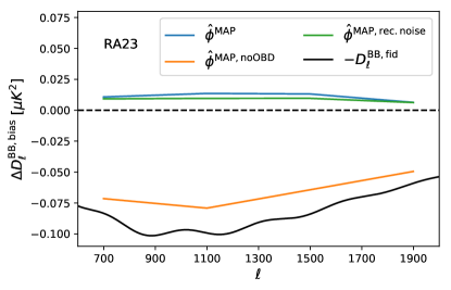
Figure 1: Total delensing bias (defined as the result of the internal delensing operation applied to Gaussian CMB simulations) in our $\hat{\phi}^{\rm MAP}$ analysis (blue line) of RA23. The contribution due to the noise of $\hat{\phi}^{\rm MAP}$ acting on the $E$-mode template is shown in green. The delensing bias one would obtain without the overlapping $B$-modes deprojection (orange line) approaches the amplitude of $D_{\ell}^{\rm BB}$ of our fiducial cosmology (black line), mimicking perfect delensing.

$B^{t}$ is built out of three CMB fields: $E^{t}$, $E^{\rm WF}$, and $B^{\rm WF}$, where the last two are used to estimate $\hat{\phi}_{{\bm{L}}}$. In a standard QE implementation the leading contribution to the internal delensing bias (though not all of it at low-noise levels Namikawa (2017)) is sourced by the disconnected (Gaussian) correlation functions involving four CMB fields. The leading contributing terms in the spectrum[$(B^{\rm dat}-B^{t})^{2}$, schematically] have the form $[E^{\rm t}\star\hat{\phi}^{\rm noise}(E^{\rm WF},B^{\rm WF})]\cdot B^{\rm dat}$, where $\star$ denotes the template building operation, the center dot $(\cdot)$ denotes the cross-spectrum between the template and the data, and $\hat{\phi}^{\rm noise}$ being the noise of the lensing tracer reconstructed using the EB estimator. Following Ref. Carron et al. (2017), we compute the delensing bias as $\Delta\hat{D}_{\ell_{b}}^{\rm BB,bias}\equiv\langle\Delta\hat{D}_{\ell_{b}}^{\rm BB}\rangle_{G}$, where $\langle\cdot\rangle_{G}$ denotes that the entire internal delensing operation is performed on Gaussian simulations, and averaged over. Since the simulations are Gaussian, the estimated lensing tracers are pure noise, and this term captures these disconnected correlators. In Fig. 1 we show the MAP $\Delta\hat{D}_{\ell_{b}}^{\rm BB,bias}$ for the RA23 data (the QE curves are similar). If no OBD is performed we see a strong negative signal similar to our negative fiducial $D_{\ell}^{\rm BB}$, creating the illusion of an almost perfect delensing (orange line). OBD prevents correlating overlapping modes in $B^{\rm WF}$ and $B^{\rm dat}$, reducing the entire bias by almost an order of magnitude (blue). Were the tracer noise statistically independent of the map being delensed, we would only see the (positive) B-power induced by the remapping of $P^{(E^{t})}$ by the tracer noise (green). This contribution can be quantified by delensing each simulation realization with an independent MAP tracer. The dominant residual contribution to the delensing bias after OBD is mostly sourced by this term, owing to $B$-modes at $\ell_{B}>2500$ leaking to lower $\ell_{B}$ in both $B^{\rm WF}$ and $B^{\rm dat}$ due to the presence of the mask which convolves different angular scales. We verified this directly with the help of another, simpler set of simulations where all modes above $\ell_{B}>2500$ were artificially zeroed out prior the analysis.

Results.​ $-$​

We build debiased band powers according to

$$\Delta\hat{D}_{\ell_{b}}^{\rm BB,debiased}=\Delta\hat{D}_{\ell_{b}}^{\rm BB}-\Delta\hat{D}_{\ell_{b}}^{\rm BB,bias}.$$ (3)

In Fig. 2 we show the inverse-variance weighted combination of $\Delta\hat{D}_{\ell}^{\rm BB,debiased}$ in the POLARBEAR patches. Table 1 shows the values of the amplitude $\Delta A^{\rm delens}$ of the simulation predictions of $\Delta\hat{D}_{\ell_{b}}^{\rm BB,debiased}$ fit to the data. By construction, these band-powers are in practice free of the internal delensing bias, and $\Delta A^{\rm delens}=0$ in the absence of lensing signatures in the data. For the patch-combined measurement, we detect a nonzero $\Delta A^{\rm delens}$ with a significance $\Delta A^{\rm delens}/\sigma_{\Delta A^{\rm delens}}$ of $5\sigma$ using $\hat{\phi}^{\rm QE}$, consistent with simulation predictions ($\Delta A^{\rm delens}=1$). The significance of the patch-combined measurement increases to $5.3\sigma$ using $\hat{\phi}^{\rm MAP}$. Our deepest patch RA23 alone provides a $4\sigma$ measurement.

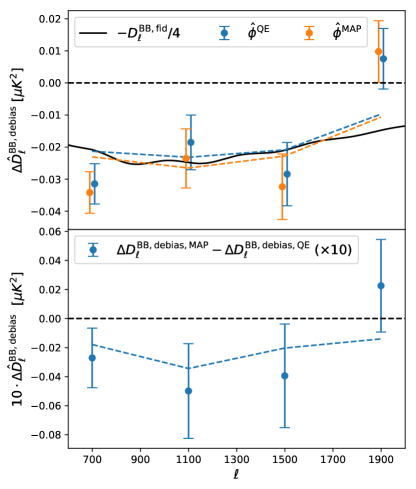
Figure 2: Top: Inverse-variance combination of the debiased spectral differences $\Delta\hat{D}_{\ell}^{\rm BB,debiased}$ measured in the POLARBEAR sky patches using QE (blue) and MAP (orange) delensing. The dashed lines show expectations obtained as average of results computed on simulations. Bottom: Difference between MAP and QE delensed $\Delta\hat{D}_{\ell}^{\rm BB,debiased}$ compared to simulation expectations (dashed lines). As both these quantities are highly correlated, the error bar of this statistic is significantly reduced when compared to those of the top panel. The significance of this difference being nonzero is $2.1\sigma$.

$\Delta\hat{D}_{\ell_{b}}^{\rm BB,debiased}$	$\Delta A^{\rm delens}[\hat{\phi}^{\rm QE}]$	$\Delta A^{\rm delens}[\hat{\phi}^{\rm MAP}]$
RA23	1.26 $\pm$ 0.33	1.38 $\pm$ 0.32
RA12	1.16 $\pm$ 0.39	1.09 $\pm$ 0.37
RA4.5	0.79 $\pm$ 0.59	0.59 $\pm$ 0.57
Patch combined	1.22 $\pm$ 0.24	1.24 $\pm$ 0.23

Table 1: Fit of the amplitude $\Delta A^{\rm delens}$ of the simulation prediction to the debiased delensed spectrum difference $\Delta\hat{D}_{\ell_{b}}^{\rm BB,debiased}$. Error bars were calculated using the Gaussian simulation set. A nonzero delensing signal is measured at more than $5\sigma$ after combining the data of all patches, consistent with simulation predictions $(\Delta A^{\rm delens}=1)$.

In all cases, $\Delta A^{\rm delens}$ agrees with expectations from simulations (shown as dashed line in Fig. 2), where the MAP delensing always outperforms QE. While MAP delensing does increase the significance of our results, we see evidence for the improvement over QE in the data only at modest significance. The difference of $\Delta\hat{D}_{\ell_{b}}^{\rm BB,debiased}$ computed with MAP and QE is nonzero at $2.1\sigma$ significance, consistent with simulation expectations. The fluctuations in this statistic are caused by the decoherence of the MAP-delensed and QE-delensed maps sourced by the slightly different noise components in the tracers. A deviation from zero of this difference is thus sourced by a difference in the delensed signal.

How much lensing $B$-mode power variance did we actually remove? The debiasing procedure subtracts $B$-power that acts as a source of additional variance in parameter inference. Hence, the relevant quantity is the reduction of power without any debiasing. We find a reduction of $B$-power of 14% ($\hat{\phi}^{\rm QE}$) and 22% ($\hat{\phi}^{\rm MAP}$) for our deepest patch RA23, in agreement with simulation expectations [$(13\pm 9)\%$ and $(15\pm 9)\%$, respectively, for its mean value]. It is more difficult to distinguish the QE from the MAP result without debiasing on real data or on a single realization of the simulations. The observed difference between MAP and QE is thus measured at only $1.1\sigma$, down from $2.1\sigma$ when performing debiasing. For MAP, RA12 and RA4.5 achieved a 15% and 1% power reduction consistent with QE results.

Robustness and consistency tests.​ $-$​

We test the consistency between $\Delta\hat{D}_{\ell_{b}}^{\rm BB}$ of data and simulations using templates built with different tracers. We subtract from $\Delta\hat{D}_{\ell_{b}}^{\rm BB}$ measured on the data the average of the same quantity computed with the non-Gaussian simulations $\left\langle\Delta\hat{D}_{\ell_{b}}^{\rm BB}\right\rangle$ and fit to these band powers the amplitude parameter $\Delta A^{\rm BB}$ of the fiducial binned $-D_{\ell}^{\rm BB}$. By construction, $\Delta A^{\rm BB}=0$ indicates a delensed $B$-power consistent with simulation expectations. We also build $\chi^{2}$’s from $\Delta\hat{D}_{\ell_{b}}^{\rm BB}$ as follows: with $\Sigma_{bb^{\prime}}$ the covariance of $\Delta\hat{D}_{\ell_{b}}^{\rm BB}$ computed from the non-Gaussian simulations, we compute the data $\chi^{2}$ across all multipole bins $b$,

$$\chi^{2}\!\equiv\!\sum_{b,b^{\prime}}\!\left(\!\Delta\hat{D}_{\ell_{b}}^{\rm BB}\!-\!\left\langle\!\Delta\hat{D}_{\ell_{b}}^{\rm BB}\!\right\rangle\!\right)\!\Sigma^{-1}_{bb^{\prime}}\!\left(\!\Delta\hat{D}_{\ell_{b^{\prime}}}^{\rm BB}\!-\!\left\langle\!\Delta\hat{D}_{\ell_{b^{\prime}}}^{\rm BB}\!\right\rangle\!\right),$$ (4)

that we turn into probability-to-exceed (PTE) values from the empirical ranking of the data $\chi^{2}$ compared to the results obtained for the simulations. Part of the noise and cosmic variance cancels in $\Delta\hat{D}_{\ell_{b}}^{\rm BB}$, and this spectral difference is constrained about 4 times better (empirically) than the band powers themselves. In addition to $\hat{\phi}^{\rm QE}$, $\hat{\phi}^{\rm MAP}$, and $\hat{\phi}^{\rm MAP}-\hat{\phi}^{\rm QE}$ tracers, we used $\hat{\phi}^{\rm QE}$ removing modes $L>500$ ($\hat{\phi}^{\rm QE,lowpass}$) to assess the impact of unmodeled tracer noise. To test for delensing bias we used a QE tracer $\hat{\phi}^{\rm QE,noOBD}$ built without OBD. Furthermore, we used tracers uncorrelated or anticorrelated with LSS, such as the lensing curl mode estimate $\hat{\omega}$ Pratten and Lewis (2016); Fabbian et al. (2018); Marozzi et al. (2016) (expected to be pure noise at our noise levels), $-\hat{\phi}^{\rm QE}$, and a QE tracer $\hat{\phi}^{\rm QE,\rm indep}$ estimated from an independent simulation. This is independent from the map to delens, but has otherwise the same statistical properties. All these should produce no delensing and an increase of B-power after template subtraction.

$\Delta\hat{D}^{\rm BB}_{\ell_{b}}-\langle\Delta\hat{D}_{\ell_{b}}^{\rm BB}\rangle$	RA23 $\Delta A^{\rm BB}$	RA12 $\Delta A^{\rm BB}$	RA4.5 $\Delta A^{\rm BB}$	RA23 PTE	RA12 PTE	RA4.5 PTE
$\hat{\phi}^{\rm QE}$	$\phantom{-}0.01\pm 0.12$ (0.13)	$\phantom{-}0.09\pm 0.13$ (0.10)	$-0.02\pm 0.15$ (0.05)	4%	60%	58%
$\hat{\phi}^{\rm MAP}$	$\phantom{-}0.07\pm 0.12$ (0.15)	$\phantom{-}0.04\pm 0.14$ (0.11)	$-0.05\pm 0.15$ (0.06)	4%	84%	75%
$\hat{\phi}^{\rm QE,lowpass}$	$-0.01\pm 0.10$ (0.13)	$\phantom{-}0.08\pm 0.12$ (0.10)	$-0.02\pm 0.13$ (0.07)	16%	39%	77%
$\hat{\phi}^{\rm MAP}-\hat{\phi}^{\rm QE}$	$\phantom{-}0.04\pm 0.04$ (0.01)	$-0.07\pm 0.04$ (0.02)	$-0.04\pm 0.04$ (0.02)	47%	17%	70%
$\hat{\phi}^{\rm QE,noOBD}$	$-0.01\pm 0.16$ ($1.10$)	$\phantom{-}0.01\pm 0.19$ (1.09)	$-0.20\pm 0.22$ (1.04)	14%	80%	76%
$\hat{\omega}^{\rm QE}$	$-0.18\pm 0.12$ ($-0.18$)	$-0.11\pm 0.13$ ($-0.14$)	$\phantom{-}0.22\pm 0.13$ ($-0.10$)	13%	3%	22%
-$\hat{\phi}^{\rm QE}$	$\phantom{-}0.05\pm 0.19$ ($-0.42$)	$-0.29\pm 0.18$ ($-0.29$)	$\phantom{-}0.07\pm 0.17$ ($-0.19$)	7%	14%	46%
$\hat{\phi}^{\rm QE,indep}$	$\phantom{-}0.06\pm 0.10$ ($-0.13$)	$\phantom{-}0.03\pm 0.10$ ($-0.10$)	$-0.05\pm 0.11$ ($-0.06$)	62%	5%	98%

Table 2: Consistency tests between delensing observed on data $\Delta\hat{D}^{\rm BB}_{\ell_{b}}$ and simulations expectations $\langle\Delta\hat{D}_{\ell_{b}}^{\rm BB}\rangle$ for different lensing tracers. For each patch we show the results of the fit of the amplitude $\Delta A^{\rm BB}$ of our fiducial $-D_{\ell}^{\rm BB}$ to $\Delta\hat{D}^{\rm BB}_{\ell_{b}}-\langle\Delta\hat{D}_{\ell_{b}}^{\rm BB}\rangle$, as well as the $\chi^{2}$ PTEs for the consistency of such quantity with a null power spectrum. $\Delta A^{\rm BB}$ fitted to $\langle\Delta\hat{D}_{\ell_{b}}^{\rm BB}\rangle$ (which includes the delensing bias) is shown in parentheses. $\Delta A^{\rm BB}>0$ means a reduction of $B$-power.

Table 2 shows the summary of our tests. $\Delta A^{\rm BB}$ amplitudes show no visible bias with respect to our simulations but we observe PTE values below 5%, notably in RA23. As all these tests are correlated we assessed the significance of these low PTEs simulating 20,000 realizations of all the band powers included in our test suites starting from their empirical covariance matrix estimated from our non-Gaussian simulations, and repeating the $\chi^{2}$ analysis. We found that the probability of observing three PTEs lower than 4% in our test suite is 11% and thus concluded that our data’s low PTEs are not significant.

Galactic foregrounds and systematics.​ $-$​

Polarized dust emission could affect delensing, for example by adding Gaussian power to the tracer noise, and hence reducing the delensing efficiency. Since the dust angular power spectrum falls sharply with multipole $\ell$ and we use only $\ell_{B}\geq 500$, we expect this effect to be small. The lensing estimator could also capture specific trispectra signatures in the highly non-Gaussian dust emission, which would propagate in lensing reconstruction and, later, delensing if uncorrected for. Preliminary studies suggest that at 150 GHz this effect is not important (Challinor et al., 2018). It is implausible for such a signature to match the LSS deflection field; so this would also act to reduce the delensing efficiency. We quantified the expected impact of small-scale Gaussian polarized dust emission in our measurement by adding to our simulated datasets a template of this emission at our frequency produced with Model 1 of the PySM package Thorne et al. (2017), itself based on Planck COMMANDER templates Adam et al. (2016). Comparing simulated $\Delta\hat{D}_{\ell_{b}}^{\rm BB}$ with and without dust we found a bias smaller than 1% of the statistical error in all multipole bins. We ignored polarized galactic synchrotron contamination as it is subdominant in PB17 Ade et al. (2017). Instrumental systematics effects in the POLARBEAR measurements of $D_{\ell}^{\rm BB}$ and QE reconstruction were found to be negligible with respect to statistical uncertainties Ade et al. (2017); Aguilar Faúndez et al. (2019).

Conclusions.​ $-$​

Our analysis has achieved the highest internal $B$-mode delensing efficiencies to date, and is the first where the lensing tracer has been built from CMB polarization alone, serving as a proof of concept for future experiments where CMB polarization rather than temperature power will dominate the lensing tracer sensitivity. This work provides the first demonstration on deep polarization data that superior delensing efficiencies can indeed be achieved using iterative delensing methods Hirata and Seljak (2003); Carron and Lewis (2017). This is a crucial step toward an efficient exploitation of future high-sensitivity $B$-mode polarization experiments of the next decade Abazajian et al. (2016); Ade et al. (2019); Suzuki et al. (2018), for which iterative methods will provide close-to-optimal constraints on the physics of inflation Carron (2019).