The Berkeley sample of Type II supernovae: $BVRI$ light curves and spectroscopy of 55 SNe II

Abstract

In this work, $BVRI$ light curves of 55 Type II supernovae (SNe II) from the Lick Observatory Supernova Search program obtained with the Katzman Automatic Imaging Telescope and the 1 m Nickel telescope from 2006 to 2018 are presented. Additionally, more than 150 spectra gathered with the 3 m Shane telescope are published. We conduct an analyse of the peak absolute magnitudes, decline rates, and time durations of different phases of the light and colour curves. Typically, our light curves are sampled with a median cadence of 5.5 days for a total of 5093 photometric points. In average $V$-band plateau declines with a rate of 1.29 mag (100 days)^-1, which is consistent with previously published samples. For each band, the plateau slope correlates with the plateau length and the absolute peak magnitude: SNe II with steeper decline have shorter plateau duration and are brighter. A time-evolution analysis of spectral lines in term of velocities and pseudoequivalent widths is also presented in this paper. Our spectroscopic sample ranges between 1 and 200 days post-explosion and has a median ejecta expansion velocity at 50 days post-explosion of 6500 km s^-1 (H$\alpha$ line) and a standard dispersion of 2000 km s^-1. Nebular spectra are in good agreement with theoretical models using a progenitor star having a mass $<16$ ${\rm M}_{\odot}$. All the data are available to the community and will help to understand SN II diversity better, and therefore to improve their utility as cosmological distance indicators.

1 Introduction

Type I and Type II supernova (SN) classification was initially established by Minkowski (1941) on the presence or absence of Balmer features in their spectra (see Filippenko 1997 for a review). Type II supernovae (hereafter SNe II) are known to be the final explosion of a massive star with an extensive hydrogen envelope (Smartt 2015 for a review).

The majority of the SN II progenitors have been constrained first using hydrodynamical models (Grassberg et al., 1971; Falk & Arnett, 1977) and local host-galaxy environment studies (Huang, 1987; van Dyk, 1992), and then later confirmed by direct progenitor detections (Van Dyk et al., 2003; Smartt et al., 2009; Fraser et al., 2012; Smartt, 2015; Van Dyk et al., 2019). It is now well accepted that SN II progenitors are the explosion of only one stellar population (red supergiants) with a zero-age main sequence mass between 8 ${\rm M}_{\odot}$ and $\sim$ 20 ${\rm M}_{\odot}$.

Based on photometric properties, SNe II were classified into two subgroups: SNe IIP characterised by a phase of constant luminosity and SNe IIL with a linear light-curve decline (Barbon et al., 1979). However, recently, large SN II sample studies have questioned this sub-classification and have suggested that the SN II family forms only one continuous group (Anderson et al., 2014; Sanders et al., 2015; Valenti et al., 2016; Galbany et al., 2016; de Jaeger et al., 2018a). Therefore, in this manuscript, SNe IIP and SNe II are referred to as SNe II.

As SN II progenitors are better understood than any other type of SN (e.g., no direct for SN Ia progenitor) and because SNe II are the most abundant SN type in nature ($\sim 60$% Li et al. 2011a), over the last two decades the SN community has demonstrated a growing interest in studying their properties and using them as metallicity (Dessart et al., 2014; Anderson et al., 2016) or standard candles (e.g., Hamuy & Pinto 2002). SN II standardisation using different methods, has shown promising results to measure extragalactic distances: the “expanding photosphere method” (Kirshner & Kwan, 1974), the “standard candle method” (Hamuy & Pinto, 2002; Nugent et al., 2006; Poznanski et al., 2009; Olivares E. et al., 2010; D’Andrea et al., 2010; Poznanski et al., 2010; de Jaeger et al., 2017a; Gall et al., 2018), the “photospheric magnitude method” (Rodríguez et al., 2014; Rodríguez et al., 2019), and the “photometric colour method” (de Jaeger et al., 2015, 2017b). Moreover, techniques for measuring extragalactic distances using independent methods (such as those afforded by SNe II) have grown increasingly important in light of recent results showing 4.4$\sigma$ disagreement between local measurements (using SNe Ia; Riess et al. 2016, 2018; Riess et al. 2019) of the local Hubble-Lemaitre constant and that inferred from the cosmic microwave background radiation (CMBR) assuming a $\Lambda$CDM cosmology (Planck Collaboration et al., 2016).

However, the distance precision derived using SNe II is still worse than that obtained with SNe Ia. The dispersion could arise from intrinsic progenitor properties like the mass of the H envelope, the metallicity, the radius, or the characteristics of circumstellar material (CSM) around the progenitor. For example, in the last few years, several studies have shown that the majority of SNe II at early epochs present evidence of CSM interactions (e.g., Khazov et al., 2016; Morozova et al., 2016; Yaron et al., 2017; Moriya et al., 2017; Dessart et al., 2017; Morozova et al., 2017; Forster et al., 2018). Moreover, some SNe II with strong CSM interaction have proven to be poor standard candles (de Jaeger et al., 2018a).

Even if individual SN II studies can be found in the literature as for example: SN 1999em (Hamuy et al., 2001; Leonard et al., 2002a; Elmhamdi et al., 2003), SN 1999gi (Leonard et al., 2002b), SN 2004et (Sahu et al., 2006; Maguire et al., 2010), SN 2005cs (Pastorello et al., 2009), SN 2013by (Valenti et al., 2015), SN 2013ej (Valenti et al., 2014; Bose et al., 2015; Huang et al., 2015; Mauerhan et al., 2017; Dhungana et al., 2016)), and SN 2016esw (de Jaeger et al., 2018b), only a small fraction of large SN II samples have been published (Hamuy, 2003; Arcavi et al., 2012; Anderson et al., 2014; Faran et al., 2014a, b; Spiro et al., 2014; Sanders et al., 2015; Galbany et al., 2016; Valenti et al., 2016; Hicken et al., 2017; Gutiérrez et al., 2017). Investigating large samples is indispensable for understanding the underlying causes of the differences in spectroscopic and photometric properties and thus for improving the current methods for deriving precise extragalactic distances.

In this work, we pursue the recent effort to do statistical analyses of large samples to better understand SN II diversity. For this purpose, we use photometric and spectroscopic observations of 55 local SNe II obtained by the UC Berkeley SN group. During the past two decades and under the Lick Observatory Supernova Search (Filippenko et al., 2001; Leaman et al., 2011, LOSS), the UC Berkeley SN group has been one of the most active groups in SN discoveries ($\sim 40$% of nearby SNe during the years 1998–2008; a smaller fraction thereafter, with the advent of wide-angle SN surveys). Their efforts have permitted the building of large datasets of any type of SN and led to the publications of a wide range of studies: SNe Ia (Ganeshalingam et al., 2010; Silverman et al., 2012a, b, c; Silverman & Filippenko, 2012; Zheng et al., 2017), SN rates (Li et al., 2011a; Shivvers et al., 2017; Graur et al., 2017b; Graur et al., 2017a), stripped-envelope supernovae (Matheson et al., 2001; Shivvers et al., 2019), SNe IIn (Bilinski et al., 2015), and SN II (Poznanski et al., 2009, 2010; Faran et al., 2014a, b; Silverman et al., 2017). However, even if a few individual objects have been published recently in the literature, such as SN 2009kr (Elias-Rosa et al., 2010), SN 2010id (Gal-Yam et al., 2011), and SN 2013ej (Dhungana et al., 2016), not all of the SN II photometric and spectroscopic data gathered by the UC Berkeley SN group since Faran et al. (2014a, b) have been published.

Therefore, the purpose of this paper is to report SN II photometric and spectroscopic data obtained by our group since 2005 and the last SN II Berkeley data sample release by Faran et al. (2014a, b). All the dataset will be immediately available to the community and the reader can find information on each SN in Appendix A, Table LABEL:SN_sample. Note that this paper is part of a more extensive data release, including stripped-envelope SNe (Zheng et al., in prep.) and SNe Ia (Stahl et al., in prep.).

This paper is divided as follows. Section 2 describes optical observations and data-reduction procedures; Section 3 presents an analysis of the photometric and spectroscopic properties of our sample, including light curves, colours, absolute magnitudes, velocities, and time evolution of spectral lines. Finally, Section 4 contains a summary and the conclusions.

2 Data Sample

The Berkeley SN II sample consists of 55 objects observed between 2006 and 2018 using the Lick Observatory (Mt. Hamilton, CA) facilities. Among these transients, 30 were discovered by LOSS (Filippenko et al., 2001). For almost all the SNe, spectra were obtained using the 3 m Shane Lick telescope and the Keck-I/Keck-II 10 m telescopes in Hawaii (see Section 2.2). However, for 9 SNe II our group did not obtain any spectra, and therefore we complete our spectroscopic sample with spectra available in the literature.

The heliocentric redshifts were obtained from the host-galaxy recession velocities published in the NASA/IPAC extragalactic Database (NED) when available, otherwise from the SN spectra. The redshift distribution of the Berkeley SN II sample is presented in Figure 1; the redshift ranges from 0.0022 (SN 2013ej) to 0.0559 (SN 2015O) with an average value of 0.0125 and a standard dispersion of 0.0103. Note that 29 SNe II are located in the Hubble flow ($z>0.01$). In Appendix A, Table LABEL:SN_sample, the reader can find information on each SN: its host galaxy, dust extinction from the Milky Way (MW), recession velocity, distance modulus, explosion epoch, last nondetection and detection epochs, number of photometric points and number of spectra.

For each SN, to determine the explosion date, the same methodology used by Anderson et al. (2014) or Galbany et al. (2016) was applied. When nondetections are available, the explosion date is taken as the intermediate epoch between the last nondetection and the first detection, and its uncertainty corresponds to half of this duration. When nondetections are not available, the explosion date is obtained using SNID (Blondin & Tonry, 2007) by matching SN II spectral templates with well-constrained explosion epochs. The explosion date is then taken as the average epoch of the best fits and its uncertainty as the standard deviation (Gutiérrez et al., 2017). Note that three SNe II (SN 2016bkv, SN 2018aoq, SN 2018bek) observed by our group will be published in more detailed studies (Van Dyk et al., in prep.; Lymin et al., in prep.).

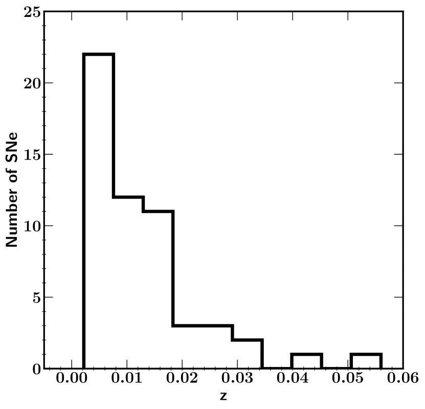
Figure 1: In this figure shows the redshift distribution of the 55 SNe II. The average value of the distribution is 0.0125 with a standard deviation of 0.0103. 29 SNe II have $z>0.01$.

2.1 Photometry

SN images were obtained using the 0.76 m Katzman Automatic Imaging Telescope (KAIT) and the 1 m Nickel telescope, both at Lick Observatory (average seeing $\lesssim 2$″). The majority of our images ($\sim 65$%) were taken with the completely robotic KAIT telescope and an exposure of 60 s in $BVRI$, while the exposure times for the Nickel images average 600 s and 300 s for $B$ and $VRI$, respectively. For more information concerning the transmission curves and the colour terms for the KAIT and Nickel telescopes, the readers are referred to Stahl et al. 2019 (in prep.).

The photometric reductions are fully described by Stahl et al. 2019 (in prep.); here we only briefly summarise the procedure. Using our automated image-reduction pipeline (Ganeshalingam et al. 2010 and Stahl et al. 2019 (in prep.)), we applied to all of the images bias removal, flat-field corrections, and astrometric solution. A majority of SNe ($\sim 60$%) were relatively close from their host galaxy, and therefore, to remove the host-galaxy luminosity, galaxy subtraction were required. Subtraction templates were obtained on a dark night using the Nickel telescope and after the SN had faded beyond detection (generally at least 1 yr after the discovery).

Finally, using DAOPHOT (Stetson, 1987) from the IDL Astronomy User’s Library, point-spread-function (PSF) photometry was performed to to measure the SN flux relative to local standard stars in the same field. Instrumental magnitudes were calibrated using two or more standard stars (depending on the field) from the Pan-STARRS1 Surveys (Chambers et al., 2016; Schlafly et al., 2012, PS1). ‎$grizy$ PS1 magnitudes were transformed into the Landolt standard system (Landolt, 1992) using the transformations given by Tonry et al. (2012). Finally, the transformation between the standard Landolt system into instrumental magnitudes was achieved using the following equations:

$$b =B+C_{B}(B-V)+{\rm constant},$$ (1a)

$$v =V+C_{V}(B-V)+{\rm constant},$$ (1b)

$$r =R+C_{R}(V-R)+{\rm constant},~{}{\rm and}$$ (1c)

$$i =I+C_{I}(V-I)+{\rm constant},$$ (1d)

where lower-case and upper-case bandpass letters are (respectively) the instrumental magnitudes and the Landolt magnitudes. The coefficient $C_{i}$ ($i=B,V,R,I$) represent the average colour terms published by Ganeshalingam et al. (2010) and Stahl et al. 2019 (in prep.). Note that there are no atmospheric effects or zero points, as they are absorbed into the constant. Finally, it is worth noting that the SN II photometry is released in the natural system of the KAIT and Nickel telescopes (transmission curves are available in Stahl et al. 2019 in prep.).

2.2 Spectroscopy

Optical spectra were obtained using the Kast double spectrograph (Miller & Stone, 1993) on the 3 m Shane telescope at Lick Observatory (155/213 spectra), the Low Resolution Imaging Spectrometer (LRIS; Oke et al. 1995) mounted on the Keck-I 10 m telescope (16/213 spectra) located on Maunakea (Hawaii), and the DEep Imaging Multi-Object Spectrograph (DEIMOS Faber et al. 2003) mounted on Keck-II 10 m telescope also located on Maunakea (7/213 spectra). To minimise light losses due to atmospheric dispersion, all of the specta were obtained at (or near) the parallactic angle (Filippenko, 1982).

To reduce our spectroscopic data, we use two fully automated public pipelines: TheKastShiv for Kast spectra and LPIPE to reduce LRIS longslit spectrum (Perley, 2019). Briefly, these two pipelines follow standard spectroscopic reduction techniques. First, the spectra were debiased, flat-field, and cleaned of cosmic rays. Then, one dimensional spectra were extracted and calibrated using lamps. Finally, spectrophotometric standard stars observed on the same night are used to calibrate the flux and removed atmospheric absorption lines.

To complete the spectral analysis, 35 spectra from the literature were added to our sample. Of these 35 spectra, four (of SN 2013bu, SN 2015X, SN 2017jbj, and SN 2016cyx) were unpublished but publicly available and were downloaded from the WISeREP database; the others were obtained from the WISeREP database or from electronic links in the published manuscripts. These 35 spectra were obtained with the 2.5 m Irénée du Pont telescope using the WFCCD and the Boller and Chivens spectrographs and the 6.5 m Magellan Clay and Baade telescopes with LDSS-2 and LDSS-3 at Las Campanas Observatory (SN 2007il, SN 2009ao; Gutiérrez et al. 2017), the Australian National University 2.3 m telescope with the Wide-Field Spectrograph (SN 2012ec, SN 2014dq; Childress et al. 2016), the 1.82 m telescope at Cima Ekar with the AFOSC spectrograph (SN 2013bu, SN 2015X, SN 2017jbj), the 2.56 m Nordic Optical Telescope with the ALFOSC instrument (SN 2013ft; Khazov et al. 2016), and the Fred Lawrence Whipple Observatory 1.5 m telescope with the FAST spectrograph (SN 2016cyx). The majority of our spectra cover a wavelength range of 3600–10,000 Å with a resolution of $\sim 10$ Å.

The distribution of the number of spectra per object shown in Figure 2 peaks at one spectrum per SN and has a median value of three spectra. 17 SNe only have one spectrum, one SN has no spectrum (SN 2014cn), and $\sim 70$% of the SNe in our sample have at least two spectra. SN 2013ab and SN 2015V are the SNe with the most spectra (14), and 15 SNe have more than five spectra each.

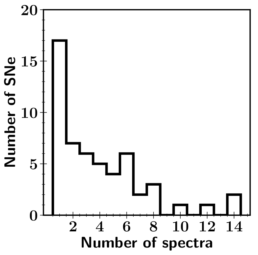
Figure 2: Black histogram represents the number of spectra per SN. In total, our sample is composed of 213 spectra and 55 SNe II.

3 Results

In this Section, we present the photometric properties (light and colour curves, absolute peak magnitudes, and slopes) and spectroscopic properties (velocities, pseudoequivalent widths) of our sample. All of these characteristics are also compared to the low-$z$ SN II samples published in the literature (Anderson et al., 2014; Galbany et al., 2016; Gutiérrez et al., 2017).

3.1 Photometric analysis

3.1.1 Light curves

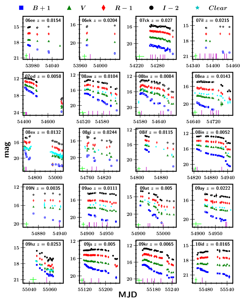
Figure 14: SN II observed light curves corrected for MW extinction. Blue squares are magnitudes in $B$, green triangles are $V$, red diamonds are $R$, and black circles are $I$. The abscissa is the Modified Julian Date (MJD). In each panel, the IAU name and the redshift are given in the upper right. Full symbols are KAIT data while empty symbols are Nickel data. The vertical magenta lines indicate the epochs of optical spectroscopy while the vertical green line represents the explosion date and its associated uncertainty.

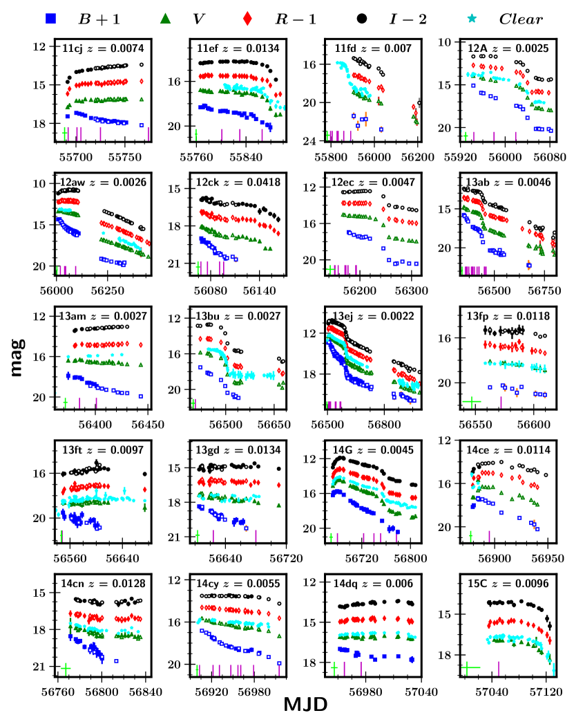
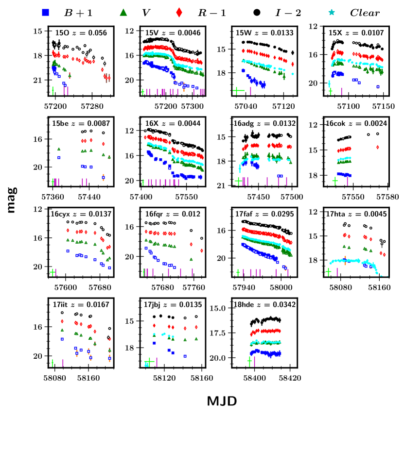
Figure 14: SN II observed light curves corrected for MW extinction. Blue squares are magnitudes in $B$, green triangles are $V$, red diamonds are $R$, and black circles are $I$. The abscissa is the Modified Julian Date (MJD). In each panel, the IAU name and the redshift are given in the upper right. Full symbols are KAIT data while empty symbols are Nickel data. The vertical magenta lines indicate the epochs of optical spectroscopy while the vertical green line represents the explosion date and its associated uncertainty.

In Figure 14, we present 55 $BVRI$ and Clear (i.e., unfiltered) light curves in the natural KAIT/Nickel photometric system. All magnitudes have been corrected for MW extinction using the dust maps of Schlafly & Finkbeiner 2011 assuming $R_{V}=3.1$ and the Cardelli et al. (1989) extinction law. We decided to not correct for host-galaxy extinction as to date no accurate methods exist to estimate it (Poznanski et al., 2011; Phillips et al., 2013; Faran et al., 2014a; Galbany et al., 2017; de Jaeger et al., 2018a). Neither $K$-corrections (Oke & Sandage, 1968; Hamuy et al., 1993; Kim et al., 1996) nor $S$-corrections (Stritzinger et al., 2002) have been applied owing to the low redshifts of our objects (see Figure 1) and the similarity between the different filters of the KAIT/Nickel system.

In Figure 3, the light-curve coverage for each SN is shown. The photometric observations start on average 12 days after the explosion with a standard deviation of 17 days. 16 SNe have their first photometric point before five days since the explosion and the vast majority of the objects before 10 days (66%). On average, the last optical images were obtained 144 days after the explosion with a standard deviation of 110 days. Two thirds of the SNe have photometric data $>100$ days after the explosion. Each SN has an average of 93 photometric points with a standard deviation of 77 points, and almost half of the SNe have at least 80 points. With 449 photometric points, SN 2013ej is the object with the best photometric coverage, followed by SN 2015V with 287 points. For SN 2006ek, we obtained only 12 optical images, our poorest sampling. The total photometric points published in this work is 5093.

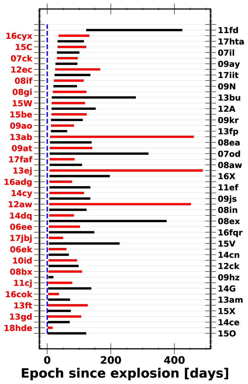
Figure 3: $BVRI$ light-curve coverage for each SN sorted by increasing first photometric observation. The vertical blue dashed line represents the explosion date.

3.1.2 Colour curves

In Figure 4, six different colour curves of the 55 SNe II are represented ($(B-V)$, $(B-R)$, $(B-I)$, $(V-R)$, $(V-I)$, and $(R-I)$). As expected, all of the colours follow the general SN II colour behaviour: at early times (30–40 days) a rapid increase is seen while at later the increase is much slower. Finally, at late epochs ($>80$–100 days) the colour curves are flatter, as they all depend on the ⁵⁶Co decay (Galbany et al., 2016). Differences in colour evolution between the different colours are also seen. The redder colours increase more slowly than the bluer colours because the red part of the spectrum is less sensitive to temperature changes than the blue part. With our LOSS sample, we do not see two distinct patterns of colour evolution in any of the colour curves, and therefore, confirming that SNe II form an unique class (Anderson et al., 2014; Sanders et al., 2015; Valenti et al., 2016; Galbany et al., 2016; de Jaeger et al., 2018a).

As described by Galbany et al. (2016), all of the colours do not show the same dispersion, with $(B-I)$ showing the largest scatter while $(R-I)$ the smallest. Galbany et al. (2016) attributed this scatter to host-galaxy dust as reddening is strongest at bluer bands. However, de Jaeger et al. (2018a) have shown that host-galaxy extinction does not seem to be the principal parameter to explain the dispersion in observed colours. They suggested that the main parameter affecting the observed colour diversity is intrinsic, depending on differences in progenitor radius and/or circumstellar material around the progenitor stars.

Even if the majority of the SN II colours diversity is intrinsic, the reddest SNe II should be affected by host-galaxy extinction. In our sample, we identify two objects (SN 2013am and SN 2016cok) whose $(B-V)$ colour differs by $>2\sigma$ from the average colour. These objects are highly extinguished: $\sim 2$ mag for SN 2013am (Tomasella et al., 2018) and $\sim 1.5$ mag for SN 2016cok (Kochanek et al., 2017). Note also that SN 2008ex shows red colours that can be explained by an unusual SN II optical light curve (after cooling the brightness increases).

Finally, following de Jaeger et al. (2018a), as $(B-V)$ colour curves can be described with one or two slopes, we perform for each SN a weighted least-squares fit of the $(B-V)$ colour curves. From our sample, the first colour slope, the second slope, and the epoch of transition have average values ($N=16$) of 2.52 $\pm$ 0.50, 0.48 $\pm$ 0.19, and 38.2 $\pm$ 5.62, respectively. These values are consistent with those published by de Jaeger et al. (2018a): 2.63 $\pm$ 0.62, 0.77 $\pm$ 0.25, and 37.7 $\pm$ 4.31. Similarly, the $(B-V)$ values at 15, 30, 50, and 70 days after the explosion are also consistent with those derived by de Jaeger et al. (2018a): 0.30 $\pm$ 0.21, 0.69 $\pm$ 0.24, 0.96 $\pm$ 0.25, and 1.06 $\pm$ 0.29, respectively. However, with this sample, we do not recover the correlation found by de Jaeger et al. (2018a) between the first and second slope. Absence of a statistically significant trend is explained by the small number of objects with good temporal coverage to see two slopes ($N=16$). To address the small number statistics issue, we add to our sample 28 SNe II from the previous LOSS SN II data release (Faran et al., 2014a, b). All these SNe II have well defined explosion dates and were observed under the same conditions (same telescopes, same pipeline). From this new sample, 14 SNe II have enough temporal coverage to see two slopes and therefore, the total SN II number increases to 30 SNe II ($N=16+14$). With this new sample, the correlation found by de Jaeger et al. (2018a) between the first and second colour slopes is confirmed with a Pearson factor of 0.54 $\pm$ 0.14 ($p\leq 2.0\times 10^{-2}$).

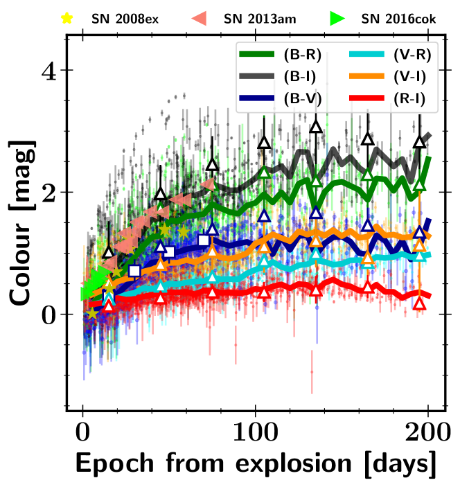
Figure 4: 55 $(B-R)$, $(B-I)$, $(B-V)$, $(V-I)$, $(V-R)$, and $(R-I)$ colour evolution corrected for MW extinction are respectively represented in green, black, blue, orange, cyan, and red. Individual measurements are shown with dots while solid lines indicate average colours in a bin size of five days. Blue squares represent the $(B-V)$ colour at 15, 30, 50, and 70 days after the explosion from the Carnegie Supernova Project-I (de Jaeger et al., 2018a). Empty triangles represent the average colour in a bin size of 30 days published by Galbany et al. (2016). The $(B-V)$ colours of SN 2008ex, SN 2013am, and SN 2016cok are respectively highlighted using yellow stars, salmon left-pointed triangles, and lime right-pointed triangles.

3.1.3 Absolute magnitudes

For each SN, absolute magnitudes are calculated using the distance modulus and the SN apparent magnitudes corrected only for MW extinction. The distance modulus is obtained using the cosmic microwave background corrected recession velocities if the value is higher than 3000 km s^-1 and assuming a $\Lambda$CDM model ($\Omega_{m}=0.3$, $\Omega_{\Lambda}=0.7$) with a Hubble constant of 70 km s^-1 Mpc^-1. An uncertainty of 300 km s^-1 is added to take into account the galaxy peculiar velocities. For recession velocities smaller than 3000 km s^-1, peculiar-motion errors are too large making the distance measurement unreliable. For these cases, following Anderson et al. (2014), the distance moduli are collected from NED (see Table LABEL:SN_sample) and based Cepheids, Tully-Fisher relation, or SN II methods.

In Figure 5, for each SN, the $BVRI$ absolute magnitude light curves are displayed in separate panels. We see that the absolute peak magnitudes spread over a wide range of $-14$ to $-18.5$ mag. The two brightest objects are SN 2017faf and SN 2012ck ($M_{V}\approx-18.5$ mag and $M_{V}\approx-18.2$ mag), while SN 2013am and SN 2016cok are the faintest objects in our sample ($\sim-14$ mag). However, as mentioned in Section 3.1.2, these two objects are highly extinguished (Tomasella et al., 2018; Kochanek et al., 2017). If we restrict our sample to the bluest objects by selecting only the SNe having an average $(B-V)$ colour less than the average $(B-V)$ colour of the whole sample, the range of absolute peak magnitude is still large ($-15$ to $-18.5$ mag). This suggests that the absolute magnitude range has an intrinsic origin in lieu of host-galaxy extinction. Note also that as demonstrated by Anderson et al. (2014) for the $V$ band and confirmed later by Sanders et al. (2015); Galbany et al. (2016) for all the bands, even if our sample shows a wide range in both absolute magnitudes and light-curve morphologies, there is no evidence of two separate subpopulations, confirming that the SN II progenitor originates from a single stellar population.

Finally, for each SN and each filter, we derive the absolute magnitude at peak brightness using a low-order polynomial fit to the photometry close to the maximum photometric point. Otherwise, for the majority of the cases, due to the absence of peak (lack of early data), the maximum brightness is taken as the first photometric point if the epoch is less than 20 days post-explosion. Our average absolute peak magnitudes excluding SN 2013am and SN 2016cok (two highly extinguished SNe) are $<B_{\rm max}>=-16.39$ mag ($\sigma=1.08$, $N=42$), $<V_{\rm max}>=-16.53$ mag ($\sigma=0.94$, $N=42$), $<R_{\rm max}>=-16.74$ mag ($\sigma=0.94$, $N=41$), and $<I_{\rm max}>=-16.95$ mag ($\sigma=0.89$, $N=42$). These values are slightly lower ($\sim 0.2$–0.3 mag) than those published by Galbany et al. (2016) but are still consistent within the uncertainties ($<B_{\rm max}>=-16.43$ mag, $<V_{\rm max}>=-16$.89 mag, $<R_{\rm max}>=-16.96$ mag, and $<I_{\rm max}>=-17.27$ mag).

The small differences above can be explained mostly by (1) the uncertainties in the SN distances (almost 20 SNe II have distances from the Tully-Fisher relation), (2) the fact that no clear maximum is seen, and therefore the first photometric point is only an approximation of the maximum, (3) observational selection effects (KAIT targets bright galaxies; Leaman et al. 2011), and (4) the uncertainties added by the host-galaxy extinction into the absolute peak magnitude values. For example, for the $V$ band, only 10 SNe II have their maximum derived from a polynomial fit. If we select only those SNe, the average absolute peak magnitudes is brighter ($-17.17$ mag). Now, if we derive the average peak magnitude only for the SNe having a recession velocity higher than 3000 km s^-1, the new values obtained are more consistent with those of Galbany et al. (2016): $<B_{\rm max}>=-16.57$ mag ($\sigma=1.14$, $N=23$), $<V_{\rm max}>=-16.74$ mag ($\sigma=0.92$, $N=23$), $<R_{\rm max}>=-16.96$ mag ($\sigma=0.85$, $N=23$), and $<I_{\rm max}>=-17.20$ mag ($\sigma=0.82$, $N=23$). Note that among the SNe having the lowest absolute peak magnitudes ($V$ band), two objects are highly extinguished (SN 2013am and SN 2016cok), while others have already been discussed in the literature such as SN 2008in (Roy et al., 2011), SN 2009N (Takáts et al., 2014), and SN 2010id (Gal-Yam et al., 2011).

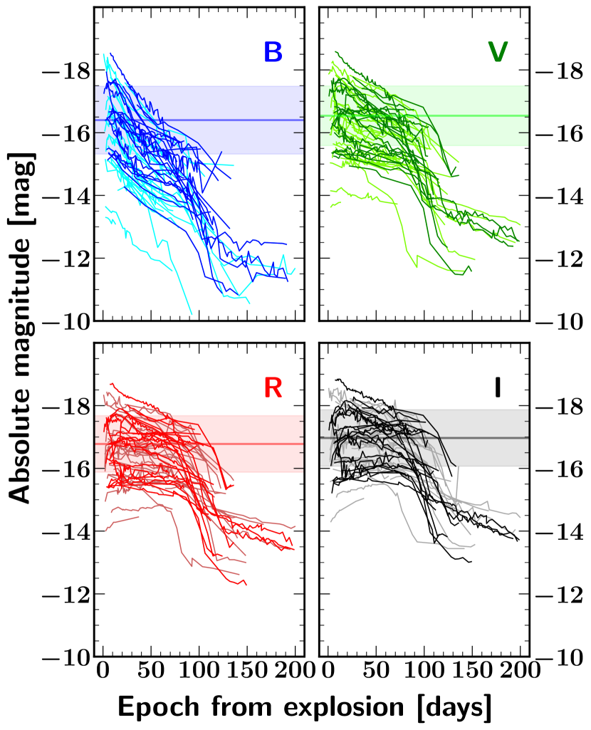
Figure 5: 55 $B$, $V$, $R$, and $I$ absolute magnitude light curves are displayed in four different panels. All the light curves have been interpolated using zero-order spline polynomials. In each panel, the darkest colours represent the SNe with the bluest $(B-V)$ colour. The horizontal line and the filled region represent the average peak magnitudes and their 1$\sigma$ uncertainties, respectively.

3.1.4 Light-curve properties

In this section, following Anderson et al. (2014) and Galbany et al. (2016), we investigate the SN II light-curve properties by measuring two different parameters: (1) the decline rate in magnitudes per 100 days between the peak brightness and the end of the plateau and (2) the optically thick phase duration (OPTd) which is equivalent to the epoch of the end of the plateau phase.

For our sample, the average plateau length in the $V$ band is 86 $\pm$ 11 days, similar to those published by Anderson et al. (2014) and Galbany et al. (2016): 83.7 $\pm$ 16.7 days and 77.5 $\pm$ 26.3 days, respectively. With a duration of 60 days, SN 2017faf has the shortest plateau, while SN 2014cy with a duration of 104 days has the largest OPTd. For $s_{1}$, $s_{2}$, $s_{3}$, and $s$ we derive respective average values of 2.60 mag (100 days)^-1 ($\sigma=1.10$; $N=10$), 1.29 mag (100 days)^-1 ($\sigma=0.90$; $N=45$), 1.15 mag (100 days)^-1 ($\sigma=0.35$; $N=11$), and 1.38 mag (100 days)^-1 ($\sigma=0.91$; $N=45$). These values are also consistent with those published by Anderson et al. (2014) [2.65 mag (100 days)^-1 ($\sigma=1.50$; $N=28$), 1.27 mag (100 days)^-1 ($\sigma=0.93$; $N=113$), and 1.47 mag (100 days)^-1 ($\sigma=0.82$; $N=30$)] and by Galbany et al. (2016) [1.53 mag (100 days)^-1 ($\sigma=0.91$; $N=45$)], respectively.

In Figure 6, histograms of the $s$-parameter distributions in each band are displayed. As expected, a trend is seen between the filter and the decline rate, in the sense of SNe II declining more steeply in bluer bands than in redder bands. For each band we derive an average decline rate of 3.31 mag (100 days)^-1 ($\sigma=1.49$; $N=34$), 1.38 mag (100 days)^-1 ($\sigma=0.91$; $N=45$), 0.82 mag (100 days)^-1 ($\sigma=0.73$; $N=42$), 0.57 mag (100 days)^-1 ($\sigma=0.81$; $N=45$) for $B$, $V$, $R$, and $I$, respectively. These values are similar with those published by Galbany et al. (2016). In contrast to the $s$ parameter, the OPTd values are similar for all bands, with only a slight (but not significant) increase for redder bands (85 $\pm$ 14, 86 $\pm$ 11, 87 $\pm$ 10, and 87 $\pm$ 11 days for $B$, $V$, $R$, and $I$, respectively). Note also, if we add the previous Berkeley SN II data release (Faran et al., 2014a, b) to our sample, the distributions and the average values are almost identical.

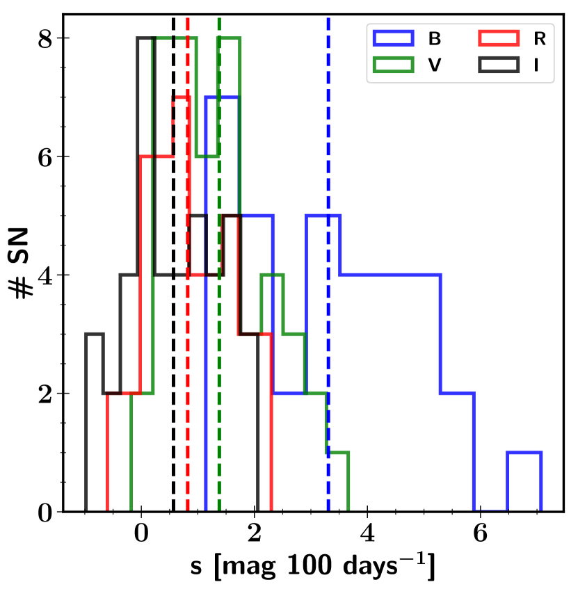
Figure 6: Histograms of the $s$-parameter distributions in each band for the Berkeley SN II sample. The vertical dashed line represents the average value. $B$, $V$, $R$, and $I$ histograms are displayed in blue, green, red, and black, respectively.

3.1.5 Brightness and decline-rate correlations

In this section, we investigate the correlation derived by various authors (Anderson et al., 2014; Sanders et al., 2015; Pejcha & Prieto, 2015; Valenti et al., 2016; Galbany et al., 2016) between the absolute peak magnitude and the plateau slope — that is, rapidly declining SNe II are generally more luminous than slowly declining SNe II. This relation has also been used to standardise SNe II and to derive extragalactic distances with a precision of $\sim 18$% (de Jaeger et al., 2015, 2017b).

In Figure 7, the absolute peak magnitude ($M$max) versus the decline rate between the maximum brightness and the end of the plateau ($s$ parameter) is plotted. In all the bands, a statistically significant correlation is seen between those two quantities, i.e., brighter SNe II decline faster. The average Pearson factors are $r_{B}=-0.56\pm 0.12$ ($N=29$, $p\leq 4.0\times 10^{-2}$), $r_{V}=-0.53\pm 0.11$ ($N=37$, $p\leq 9.0\times 10^{-3}$), $r_{R}=-0.61\pm 0.11$ ($N=33$, $p\leq 3.5\times 10^{-3}$), and $r_{I}=-0.72\pm 0.09$ ($N=34$, $p\leq 1.0\times 10^{-4}$). Our results also support the existence of the correlation between $s$ and $M$max for the $B$ band (Galbany et al., 2016), contrary to Pejcha & Prieto (2015) who do not find a correlation for bands with $\lambda<0.5\,\mu$m.

Figure 8 shows the correlation between the OPTd and the decline rate. In all the bands, the OPTd distribution ranges from $\sim 60$ to $\sim 110$ days with an average value of 86 days. From this figure, we see that SNe II with steeper decline generally have shorter plateau duration. The average slope of this correlation is $-24.964\pm 5.481$, once again consistent with the value derived by Galbany et al. (2016). However, contrary to their work, the strength of the correlation does not increase from bluer to redder bands and remains mostly similar in each band ($Pearsonfactor\pm 0.5$–0.6).

Finally, these two correlations between the decline rate and the absolute magnitude or the OPTd agree with previous observational and theoretical work (Blinnikov & Bartunov, 1993; Popov, 1993; Anderson et al., 2014; Sanders et al., 2015; Pejcha & Prieto, 2015; Valenti et al., 2016; Galbany et al., 2016). SN progenitors with smaller hydrogen envelopes have shorter OPTd because the radiation is trapped for a shorter time and are brighter as a larger fraction of radiation can escape. It is worth noting that the narrow plateau duration distribution ($\sim 15$%) could be explained by the idea that if the energy varies directly as the cube of the mass, the plateau duration only depends slightly on the radius (Poznanski, 2013).

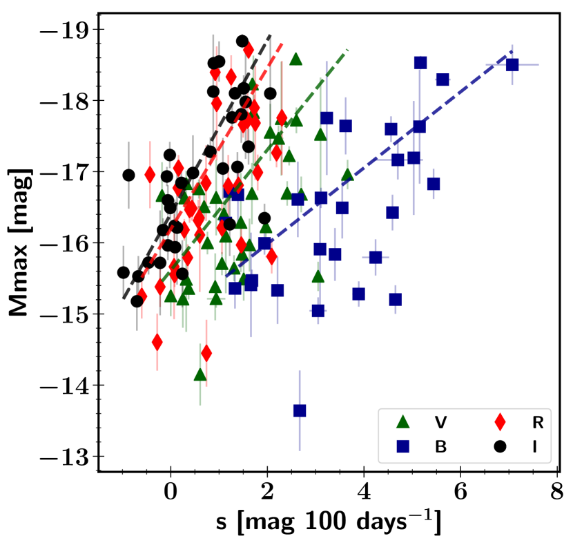
Figure 7: Absolute peak magnitudes versus the slope in mag per 100 days between the maximum brightness and the end of the plateau ($s$ parameter). Blue squares, green triangles, red diamonds, and black circles represent $B$, $V$, $R$, and $I$, respectively. In all the bands, more-luminous SNe II have steeper decline rates.

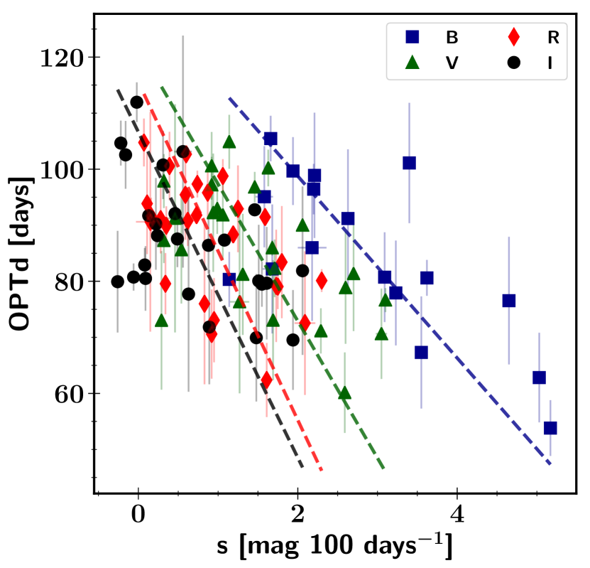
Figure 8: Optically thick duration (OPTd; plateau phase) versus decline rate in mag per 100 days between the maximum brightness and the end of the plateau ($s$ parameter). Blue squares, green triangles, red diamonds, and black circles represent $B$, $V$, $R$, and $I$, respectively. In all the bands, faster-declining SNe II have shorter OPTd.

3.2 Spectroscopic analysis

At early phases, a SN II spectrum exhibits a blue continuum (10,000 K) with strong P-Cygni profiles of Balmer lines (H$\alpha$ $\lambda 6563$, H$\beta$ $\lambda 4861$, H$\gamma$ $\lambda 4341$) and the He I $\lambda 5876$ line. With time, the SN ejecta will expand and the inner products will start to appear as (for example) Fe ii $\lambda\lambda 4924$, 5018, 5169, Na i D $\lambda\lambda 5890$, 5896, O i $\lambda 7774$, or Ca ii $\lambda\lambda 8498$, 8542, 8662 (also Sc ii, Ba ii, Ti ii; see Gutiérrez et al. 2017). Finally, the ejecta will become transparent (nebular phase), allowing the photons to escape from the core. Therefore, the spectrum will be dominated by emission lines formed by recombination or by collisional excitation such as O i $\lambda\lambda 6300$, 6364, Fe ii $\lambda 7155$, and Ca ii $\lambda\lambda 7291$, 7323.

3.2.1 Sample properties

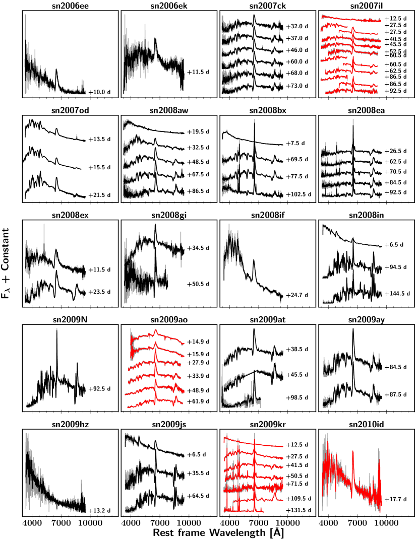
Figure 15: Spectral sequence for each SN. The spectra are shown in the rest frame, and the date listed for each SN is the number of days since the explosion (rest frame). The redshift of each SN is also labelled. The original spectra are shown in grey while in black the spectra are binned (10 Å). We represent in red the spectra that are already available the literature.

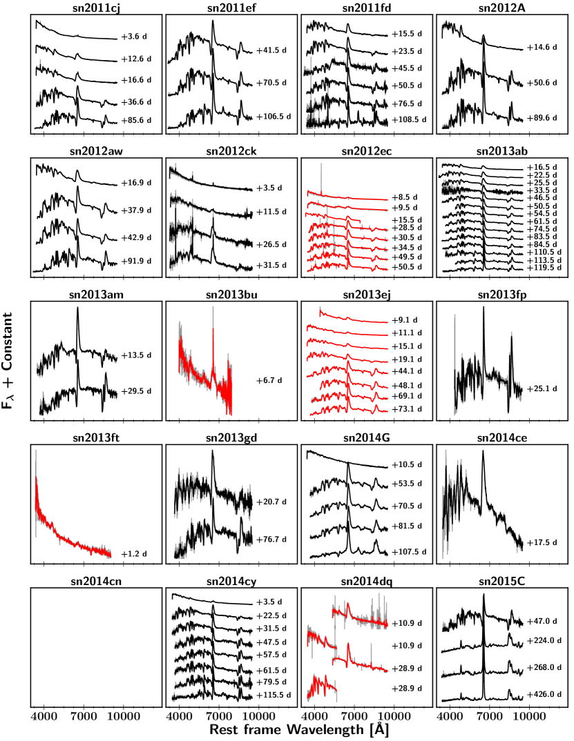
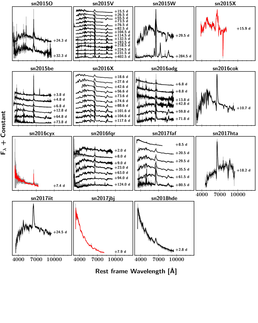
Figure 15: Spectral sequence for each SN. The spectra are shown in the rest frame, and the date listed for each SN is the number of days since the explosion (rest frame). The redshift of each SN is also labelled. The original spectra are shown in grey while in black the spectra are binned (10 Å). We represent in red the spectra that are already available the literature.

In Figure 15, we display 213 optical spectra of 55 SNe II, among which $\sim 160$ spectra from 43 SNe II are previously unpublished. The distribution of our spectroscopic sample as a function of the epoch after the explosion is displayed in Figure 9, showing that the majority (87%) of the spectra were taken $<100$ days since the explosion and only 27 spectra were obtained after 100 days. Half of the spectra were obtained during the hydrogen recombination phase, between 30 and 100 days. The earliest spectrum in our compilation corresponds to SN 2013ft (iPTF13dkk) at $1\pm 1$ days (already published by Khazov et al. 2016), followed by the unpublished SN 2016fqr spectrum at $2\pm 1.5$ days. The oldest spectrum was taken at 4$26\pm 19$ days (SN 2015C). In the same figure, we also represent for the first and last spectrum epoch (for each SN) distributions in red and blue, respectively. The majority of SNe in our compilation have their first spectra within 20 days after the explosion, with an average value of 18 days and a standard deviation of 17 days. The last spectrum was obtained on average 77 days after the explosion, and three unpublished SNe had their last spectra taken after 200 days (SN 2015C, SN 2015V, and SN 2015W), during the nebular phase.

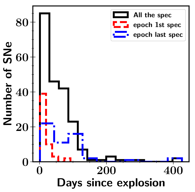
Figure 9: Black histogram represents the spectrum epoch distributions. Red-dot histogram and blue dash-dot histogram are the distributions in days of the first and the last spectrum taken for each SN, respectively.

3.2.2 Median spectra

In this section, following the work done by Liu et al. (2016) and Shivvers et al. (2019), we construct a median spectrum at different phases to investigate the spectral line variations between the different SNe II. As epochs, we choose 15, 50, 80, and $>250$ days after the explosion, corresponding to the maximum brightness, the recombination phase, the end of the plateau, and the radioactive phase, respectively. For each epoch (at $\pm 5$ days except for the radioactive phase), we select only one spectrum per SN and then correct the spectrum for the MW extinction and the redshift.

Each corrected spectrum is normalised using a pseudocontinuum defined with a cubic spline. Then, all the normalised spectra are smoothed (window of width 21 Å) and then interpolate using the same wavelength array. Finally, for each wavelength, we derive the median flux value and its median absolute deviation. In Figure 10, the median spectra at the four different epochs are displayed.

During the photospheric phase (15, 50, 80 days), most of the spectral variation is seen in the H$\alpha$ line profile and the strength of iron lines. These variations reflect the diversity of SN II progenitor properties. For example, the ratio between the absorption and the emission of the H$\alpha$ P-Cygni profile correlates with the expansion velocity (Gutiérrez et al., 2014). Similarly, Dessart et al. (2014) has shown that metal line shapes depend on the progenitor metallicity. Note also, even if some variations are seen in the median spectra during the plateau phase (50 days), almost no differences are seen between the median spectra of the slow-declining and fast-declining SNe (7/13 SNe II with $s_{2}>1.5$ mag (100 days)^-1). This is again consistent with the fact that the SNe II compose a unique group (Anderson et al., 2014; Sanders et al., 2015; Valenti et al., 2016; Galbany et al., 2016). Finally, in the nebular spectrum, the shapes of the different emission-line profiles are similar (Maguire et al., 2012a), but a variation of the strength of the forbidden emission lines (e.g., [O i] $\lambda\lambda 6300$, 6364) is seen. This scatter indicates differences in progenitor-star masses.

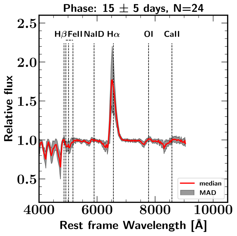
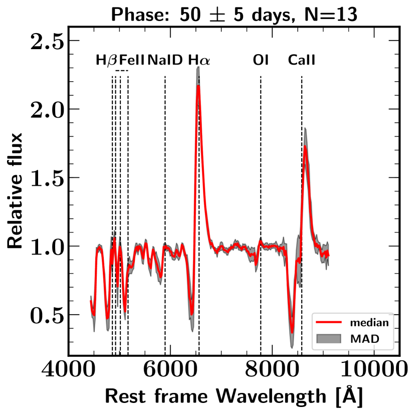
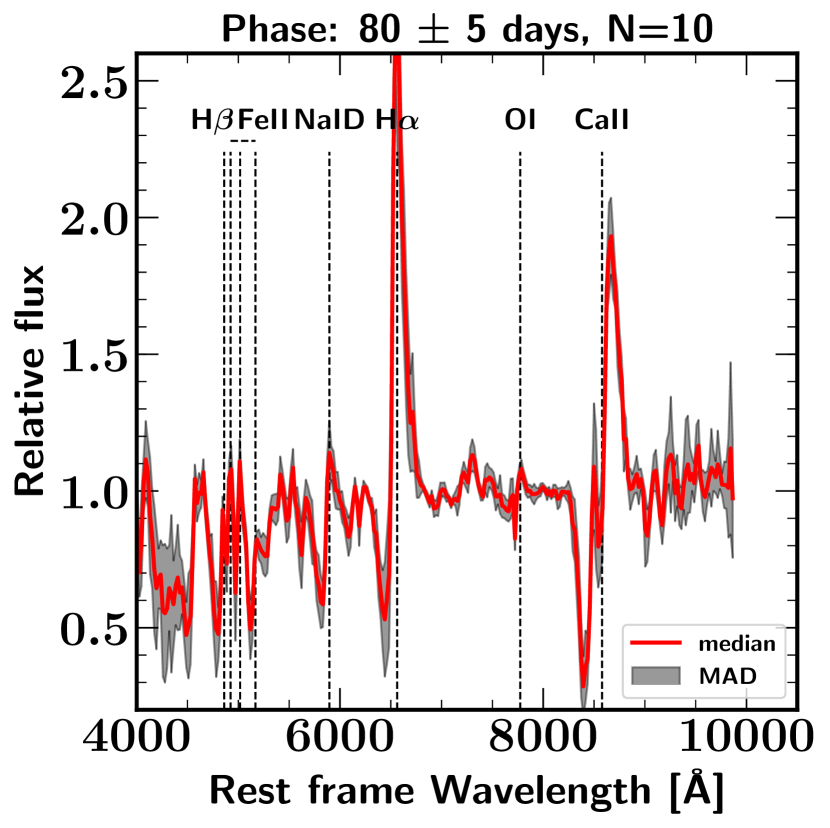
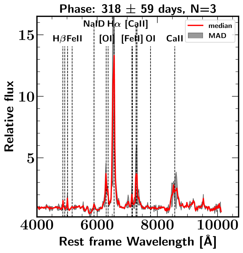
Figure 10: Median spectra at 15 $\pm$ 5, 50 $\pm$ 5, 80 $\pm$ 5, and $\sim 300$ days after the explosion are displayed. Only one spectrum per SN is included, and the number of spectra used is indicated ($N$). The median spectrum is shown in red while the median absolute deviation is in grey.

3.2.3 Absorption velocity

In this and the following (3.2.4) sections, we measure the absorption velocity and the strength of six spectral lines present during the photospheric phase. Two lines are visible throughout the whole SN spectrum evolution (H$\alpha$ $\lambda 6563$, H$\beta$ $\lambda 4861$), and four during the plateau phase (Fe ii $\lambda\lambda 4924$, 5018, 5169 and Na i D $\lambda 5893$). We also investigate the H$\alpha$ extra absorption component (also called “Cachito”; Gutiérrez et al. 2017) which is related to Si ii $\lambda 6355$ at early phases and to a high-velocity feature of H$\alpha$ at late epochs (Gutiérrez et al., 2017). Even if after 20 days, strong lines such as O i $\lambda 7774$ or the Ca ii near-infrared triplet ($\lambda\lambda 8498$, 8542, 8662) emerge in the spectrum, those lines are not included in this analysis as they are contaminated by telluric lines or result from blended lines, making it difficult to measure the pseudoequivalent width (pEW) and the velocity.

Minimum flux of the absorption of different features is used to measure the ejecta expansion velocities. The minimum flux position in wavelength is estimated using IRAF and by fitting a Gaussian profile. The position in wavelength is then transformed into velocity using the Doppler relativistic formula. To obtain velocity uncertainties, we change the continuum fit many times, measure the minimum of the absorption and determining their standard deviation. To this uncertainty, another one from the spectral resolution ($\sim 10$ Å) is also added in quadrature. All of the velocities are shown in Figure 12 together with their average evolution from the Carnegie Supernova Project-I (CSP-I) SN II sample (Gutiérrez et al., 2017).

Figure 12 shows that SN II ejecta velocities follow the typical evolution for homologous expansion (a power law; Hamuy 2001): in the ejecta, deeper material is at smaller radii and therefore moving at lower velocities. At all epochs, H$\alpha$ shows higher velocities than other lines, with a velocity starting at $\sim 10,500$ km s^-1 at early times (10 days) to $\sim 6500$ km s^-1 during the plateau phase (50 days). At 50 days, the H$\alpha$ velocity displays a large range from $\sim 8500$ km s^-1 to $\sim 4500$ km s^-1. Following H$\alpha$, H$\beta$ has the highest velocities, with a velocity ranging from $\sim 8500$ km s^-1 (10 days) to $\sim 5500$ km s^-1, on average 1000–1500 km s^-1 smaller than H$\alpha$. Finally, the iron lines exhibit the lowest velocities, with a range from $\sim 6000$ km s^-1 to $\sim 2500$ km s^-1 at 50 days. This velocity sequence (H$\alpha$ $>$ H$\beta$ $>$ Fe ii) is expected; since the H$\alpha$ and H$\beta$ lines are formed at larger radii, and therefore their velocities should be higher than those formed closer to the photosphere like the Fe ii lines (Dessart & Hillier, 2005; Takáts & Vinkó, 2012). As seen in Figure 12, our velocity measurements are consistent with those derived by Gutiérrez et al. (2017) using a low-redshift sample of 122 SNe II. For each element, the majority of our velocities are within their $1\sigma$ standard deviation (red filled region), and their average values are also similar to ours (e.g., median difference of $\sim 200$ km s^-1 for H$\alpha$).

It is also important to note that as suggested by a number of previous studies (Nugent et al., 2006; Poznanski et al., 2010; Takáts & Vinkó, 2012; de Jaeger et al., 2017b), H$\beta$ absorption is the best line for measuring the expansion velocity of the ejecta at early times or in a noisy spectrum. At early times, H$\alpha$ absorption is sometimes blended with Si ii $\lambda 6355$ (Gutiérrez et al., 2017), leading to an overestimate of the velocities ($>14,000$ km s^-1; see Figure 12); moreover, the Fe ii $\lambda$5018 line only appears later than H$\beta$ (30–40 days after the explosion), while Fe ii $\lambda$5169 is often blended with other features.

Finally, as discussed by (Gutiérrez et al., 2017), 40% of the SNe II in our compilation exhibit on the blue side of the H$\alpha$ lines an extra component between 6100 and 6300 Å at early epochs ($<40$–45 days after explosion) and between 6300 and 6450 Å at later epochs. The differences in the line shape and strength between the two phases suggest different origins: at early epochs, the extra component is associated with Si ii $\lambda 6355$, while at later epochs it is associated with a high-velocity feature of H$\alpha$ (Gutiérrez et al., 2017).

3.2.4 Absorption-line strength measurements

Absorption-line strength measurements are useful for a better understanding of SN II progenitor diversity: metal-line strength depends on progenitor metallicity (Dessart et al., 2014) and plays a role in the Hubble-diagram scatter (de Jaeger et al., 2017a). To quantify the absorption strength, we use the pEW. As for the velocities, the pEW is derived using IRAF by marking the two edges of the absorption line and defining a pseudocontinuum. Then a pixel-value integration is achieved between the two marked points.

In Figure 12, the pEW evolution for each element is displayed together with the average evolution from the CSP-I SN II sample (Gutiérrez et al., 2017, shown in red). H$\alpha$ and H$\beta$ exhibit similar evolutionary behaviour, with an increment of the pEW during the first two months from 0 to $\sim 80$ Å following by a plateau. However, as noted by (Gutiérrez et al., 2017), after $\sim 80$ days the peW decreases in a few SNe II. On the other hand, the Fe ii and Na i D pEW evolution show a steady increase with time. For Fe ii $\lambda$5169, the pEW grows from 0 to $\sim 60$ Å, becoming the strongest iron line, while the Na i D $\lambda 5893$ pEW evolves from from 0 to $\sim 90$ Å.

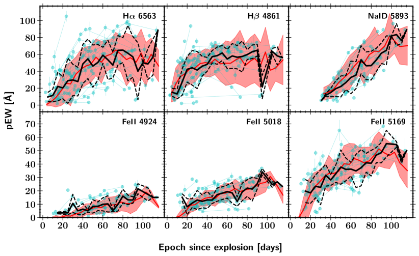
Figure 11: Expansion-velocity evolution of H$\alpha$ $\lambda 6563$, H$\beta$ $\lambda 4861$, Na i D $\lambda 5893$, and Fe ii $\lambda\lambda 4924$, 5018, 5169 are displayed (cyan circles). The black solid and dashed lines represent the average velocity in bins of five days and its standard deviation. The solid red and filled region are the average and the standard deviation derived by Gutiérrez et al. (2017) using the CSP-I sample.

Figure 12: Pseudoequivalent-width evolution of H$\alpha$ $\lambda 6563$, H$\beta$ $\lambda 4861$, Na i D $\lambda 5893$, and Fe ii $\lambda\lambda 4924$, 5018, 5169 are displayed (cyan circles). The black solid and dashed lines represent the average pEW in bins of five days and its standard deviation. The solid red and filled region are the average and the standard deviation derived by Gutiérrez et al. (2017) using the CSP-I sample.

3.2.5 Late-time spectra

After being powered by hydrogen recombination, the light curve enters a phase where the hydrogen envelope becomes transparent and the core becomes visible. At that time, the energy is produced by the radioactive decay of ⁵⁶Co into ⁵⁶Fe. The P-Cygni absorption features (indicators of an optically thick photosphere) present in the spectrum disappear, leaving a weak continuum dominated by forbidden emission lines of oxygen ([O i] $\lambda\lambda 6300$, 6364), calcium ([Ca ii] $\lambda\lambda 7291$, 7325), iron ([Fe ii] $\lambda 7155$), and lines that were present during the photospheric phase such as H$\alpha$ $\lambda 6563$ and the Ca ii near-infrared triplet ($\lambda\lambda 8498$, 8542, 8662). Nebular spectra are useful for constraining the physical properties of the SN progenitor. After carefully taking into account the primordial oxygen, the [O i] $\lambda\lambda 6300$, 6364 flux can be used to estimate the main-sequence mass of the progenitor star; larger progenitor masses lead to stronger oxygen lines (Maguire et al., 2012a; Jerkstrand et al., 2012, 2014; Dessart & Hillier, 2019).

In this section, we compare our late-time spectra to a set of theoretical nebular spectra presented by Jerkstrand et al. (2014) and Dessart et al. (2013). For the first set, four progenitor masses have been modelled (12, 15, 19, and 25 ${\rm M}_{\odot}$), while for the six models presented by Dessart et al. (2013) the mass is constant (15 ${\rm M}_{\odot}$) but the progenitor metallicity and mixing-length parameters vary.

Most of the nebular spectra from our sample have already been published by Silverman et al. (2017). However, seven spectra of three recent SNe II were previously unpublished (SN 2015C, SN 2015V, and SN 2015W). These spectra were selected based on their epochs ($>200$ days after the explosion) and visual inspection (no continuum emission or P-Cygni absorption features). We compare each spectrum to each model at the closest epoch, and select the best fit using a cross-correlation algorithm over the full wavelength range and a visual sanity check.

In Figure 13, the seven nebular spectra together with their best theoretical fits are displayed. Consistent with Jerkstrand et al. (2015) and archival prediscovery images (Smartt, 2015), our nebular spectra are in good agreement with progenitor stars having $M<16{\rm M}_{\odot}$. Even if (as noticed by Silverman et al. 2017) theoretical models generally underproduce the Ca ii NIR triplet ($\lambda\lambda 8498$, 8542, 8662) or overproduce the He i ($\lambda 7065$) emission, the strength of the [O i] $\lambda\lambda 6300$, 6364 doublet is well fitted by the 12 or 15 ${\rm M}_{\odot}$ models. It is worth noting the case of SN 2015C, where almost no spectral evolution is seen between the spectra taken 268 and 426 days after the explosion, while theoretical models show strong evolution of the [Ca ii] $\lambda\lambda 7291$, 7324 flux.

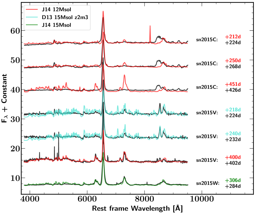
Figure 13: Eight observed nebular spectra of four SNe II from our sample (in black) are compared with theoretical models from Dessart et al. (2013) or Jerkstrand et al. (2014). The epochs of the observed spectra and the best theoretical models are shown together with the SN names.

4 Summary and Conclusions

In this work, we present a compilation of SNe II observed over the past decade by the Berkeley SN group. This sample consists of 55 optical light curves obtained with the KAIT and Nickel telescopes at Lick Observatory. Our $BVRI$ light curves start (on average) 12 days after the explosion and last until 144 days. For each band, we estimate the main photometric parameters (the absolute peak magnitude, the length of the plateau, and the slope of the plateau), and we also investigate the $(B-R)$, $(B-I)$, $(B-V)$, $(V-I)$, $(V-R)$, and $(R-I)$ colour curves. In addition to the visual-wavelength photometry, 213 spectra ranging between 1 and 426 days post-explosion are analysed. For each spectrum, we measure the absorption velocity and the strength of six spectral lines: H$\alpha$ $\lambda 6563$, H$\beta$ $\lambda 4861$, Fe ii $\lambda\lambda 4924$, 5018, 5169, and Na i D $\lambda 5893$. To study the spectral-line variations among the different SNe II, we also construct a median spectrum at four different phases (15, 50, 80, and older than 250 days after the explosion). Finally, we compare our seven previously unpublished late-time spectra to a set of theoretical nebular spectra. The main results obtained from our photometric and spectroscopic analysis can be summarised as follows.

1. Confirming earlier studies, we find that SNe IIP and SNe IIL share common photometric and spectroscopic properties and therefore, form a continuous group.

2. The absolute peak magnitudes (not corrected for host-galaxy extinction) found are $<B_{\rm max}>=-16.40$ mag ($\sigma=1.08$, $N=42$), $<V_{\rm max}>=-16.54$ mag ($\sigma=0.95$, $N=42$), $<R_{\rm max}>=-16.78$ mag ($\sigma=0.90$, $N=41$), and $<I_{\rm max}>=-16.97$ mag ($\sigma=0.90$, $N=42$).

3. Similar to previous studies (Faran et al., 2014a; Galbany et al., 2016; de Jaeger et al., 2018a), we found that redder colours (e.g., $R-I$) increase more slowly with time than the bluer colours (e.g., $B-V$) as the blue part of the spectrum is more sensitive to temperature changes. At a given epoch, the scatter among different SNe is larger for bluer colours than redder colours (cf Figure 4). This scatter could be caused by intrinsic progenitor properties or host-galaxy extinction.

4. The plateau length is similar in all the bands while the plateau slope decreases in redder filters (Sanders et al., 2015; Galbany et al., 2016).

5. For each band, the plateau slope correlates with the plateau length and the absolute peak magnitude: SNe II with steeper decline are generally brighter and have shorter plateau duration (Anderson et al., 2014; Sanders et al., 2015; Galbany et al., 2016).

6. In SN II photospheric spectra, most of the variation is seen in the H$\alpha$ feature and the strength of iron lines, reflecting the diversity of SN II progenitor properties (e.g., Gutiérrez et al. 2014; Dessart et al. 2014).

7. Consistent with (Gutiérrez et al., 2017), the pEW of H$\alpha$ and H$\beta$ increases during the first two months from 0 to $\sim 80$ Å until reaching a plateau, while the Fe ii and Na i D pEW show a steady increase with time.

8. Our nebular spectra are in good agreement with progenitor stars having $M<16{\rm M}_{\odot}$.

Note that, our photometry and spectroscopy is available for download from the Berkeley SuperNova DataBase (SNDB; Silverman et al. 2012a) or can be requested from the authors. All of the spectra are in units of $10^{-15}$ erg s^-1 cm^-2 Å^-1. The photometry is published in the natural system. The photometric error bars include only the statistical uncertainties (scatter in sky values, Poisson errors) and uncertainties in the calibration catalogue. No uncertainties associated with the host-galaxy subtraction are applied ($\sim 0.06$ mag; see Stahl et al. 2019, in prep.).

Appendix A SN II sample information, light curves, and spectra.

Table 1: Type II Supernova Sample.

SN	Host Galaxy	$A_{V}$(MW)	$v_{\rm helio}$	DM	Explosion date	Nondetect	Discovery	$\#$ Phot	$\#$ Spectra	Ref
		mag	km s-1	mag	MJD	UT	UT
SN 2006ee	NGC 774	0.167	4620	34.12(0.14)	53961.0(4)	Aug. 10.45	Aug. 18.47	30	1	Joubert & Li (2006)
SN 2006ek	MCG +04-52-3	0.213	6104	34.61(0.11)	53968.5(4)	Aug. 17.39	Aug. 25.27	12	1	Mostardi et al. (2006)
SN 2007ck	MCG +05-43-16	0.309	8083	35.32(0.09)	54228.0(13)a	06 Sep. 18	May 19.04	122	6	Boles (2007)
SN 2007il	IC 1704	0.129	6454	34.75(0.11)	54348.5(4)	Sep 2.45	Sep. 10.45	16	12b	Chu & Li (2007)
SN 2007od	UGC 12846	0.100	1734	31.91(0.80)c	54400.5(5)a	06 Oct 18	Nov 2.85	90	3	Mikuz & Maticic (2007)
SN 2008aw	NGC 4939	0.111	3110	33.48(0.18)	54517.5(10)	Feb. 11.54	Mar. 2.49	79	5	Winslow et al. (2008)
SN 2008bx	Anon.	0.065	2518	32.99(0.80)c	54576.5(4)	Apr. 9	Apr. 22.35	106	4	Puckett et al. (2008)
SN 2008ea	NGC 7624	0.366	4275	33.77(0.16)	54646.5(8)	Jun. 21.44	Jul. 6.07	81	5	Mostardi et al. (2008)
SN 2008ex	UGC 11428	0.201	3945	33.67(0.17)	54692.5(2)	Aug. 14.31	Aug. 17.32	70	2	Li & Filippenko (2008)
SN 2008gi	CGCG 415-004	0.181	7328	35.07(0.09)	54742.5(9)	Sep. 24.40	Oct. 12.41	38	2	Chu et al. (2008)
SN 2008if	MCG -01-24-10	0.090	3440	33.68(0.16)	54806.3(5)	Dec. 2.23	Dec. 12.21	24	1	Pignata et al. (2008)
SN 2008in	NGC 4303	0.061	1566	30.38(0.47)c	54824.5(2)	Dec. 23.95	Dec. 26.79	86	3	Nakano et al. (2008)
SN 2009N	NGC 4487	0.057	1036	31.49(0.40)c	54846.5(5)a	Jan. 3	Jan. 24.8	18	1	Nakano et al. (2009a)
SN 2009ao	NGC 2939	0.106	3339	33.62(0.17)	54890.1(4)	Feb. 24.12	Mar. 4.12	67	6b	Pignata et al. (2009)
SN 2009at	NGC 5301	0.047	1503	31.71(0.20)c	54900.5(8)a	05 Jan. 10	Mar. 11.63	51	3	Nakano et al. (2009b)
SN 2009ay	NGC 6479	0.117	6650	34.90(0.10)	54894.5(15)	Feb. 17	Mar. 20.41	58	2	Puckett & Peoples (2009)
SN 2009hz	UGC 11499	0.469	7572	35.16(0.08)	55043.8(3)	Jul 29.37	Aug. 3.30	42	1	Kong et al. (2009)
SN 2009js	NGC 918	0.968	1507	32.33(0.15)d	55109.5(6)	Sep. 30.44	Oct. 11.44	105	3	Nakano et al. (2009c)
SN 2009kre	NGC 1832	0.200	1939	32.08(0.25)c	55132.5(10)a	Oct. 3.76	Nov. 6.73	117	7	Nakano et al. (2009d)
SN 2010ide	NGC 7483	0.166	4939	34.10(0.14)	55452.3(3)f	Sep. 11.34	Sep. 15.24	72	1	Lin et al. (2010)
SN 2011cj	UGC 9356	0.072	2224	32.86(0.47)c	55688.4(2)	May 5.39	May 9.39	106	5	Li et al. (2011b)
SN 2011ef	UGC 12640	0.188	4009	33.60(0.18)	55759.5(1)	Jul. 16.44	Jul. 18.46	97	3	Blanchard et al. (2011)
SN 2011fd	NGC 2273B	0.201	2101	32.22(0.35)c	55782.5(10)a	Apr. 21	Aug. 20.12	53	6	Koff et al. (2011)
SN 2012A	NGC 3239	0.088	753	29.93(0.37)d	55929.4(3)	Dec. 29	Jan. 7.38	62	3	Moore et al. (2012)
SN 2012aw	NGC 3351	0.076	778	30.01(0.09)g	56002.1(1)f	Mar. 15.27	Mar. 16.9	284	4	Fagotti et al. (2012)
SN 2012ck	Anon.	0.260	12520	36.30(0.05)	56064.5(2)	May 15.50	May 19.50	125	4	Kandrashoff et al. (2012)
SN 2012ec	NGC 1084	0.073	1407	31.20(0.40)c	56142.5(9)f	$\cdots$	Aug 11.04	77	8h	Monard et al. (2012)
SN 2013ab	NGC 5669	0.075	1368	31.40(0.53)c	56339.5(1)	Feb. 15.53	Feb. 17.54	165	14	Blanchard et al. (2013)
SN 2013am	NGC 3623	0.068	807	30.54(0.40)c	56371.5(1.5)f	Mar. 20.20	Mar 21.64	86	2	Nakano et al. (2013)
SN 2013bu	NGC 7331	0.250	816	30.79(0.08)g	56399.3(4.5)	Apr. 12.8	Apr. 21.76	64	1h	Itagaki et al. (2013)
SN 2013eje	NGC 628	0.191	657	29.93(0.40)c	56496.9(1)f	Jul 14.42	Jul. 25.45	449	8	Kim et al. (2013)
SN 2013fp	IC 421	0.663	3548	33.57(0.17)	56546.9(7.5)	Sep. 4.4	Sep. 19.4	55	1	Zheng et al. (2013)
SN 2013ft	NGC 774	0.148	2907	33.66(0.29)d	56546.8(1)	Sep. 11.29	Sep. 13.29	135	1h	Fuller et al. (2013)
SN 2013gd	MCG-01-10-39	0.374	4021	33.75(0.16)	56603.3(2)	Nov. 5.3	Nov. 9.35	113	2	Casper et al. (2013)
SN 2014G	NGC 3448	0.003	1350	31.94(0.80)c	56669.5(2)	Jan. 10.85	Jan 14.32	150	5	Itagaki et al. (2014)
SN 2014ce	NGC 7673	0.119	3408	33.22(0.20)	56877.5(1)	Aug. 8	Aug. 9.52	62	1	Kim et al. (2014)
SN 2014cn	NGC 4134	0.05	3826	34.02(0.15)	56767.2(4)	Apr. 16	Apr. 24.38	113	0	Kumar et al. (2014)
SN 2014cy	NGC 7742	0.049	1663	31.73(0.80)c	56899.5(1)f	Aug 29.3	Aug 31.0	99	8	Nishimura (2014)
SN 2014dq	ESO 467-G51	0.051	1808	31.35(0.28)c	56945.6(3)	Oct. 13.09	Oct. 19.09	97	4h	Bock et al. (2014)
SN 2015C	IC 4221	0.223	2889	33.32(0.20)	57003.0(19)a	$\cdots$	Jan. 7.60	46	4	Pina et al. (2015)
SN 2015O	PGC 1426131	0.404	16788	36.98(0.04)	57194.7(1)	Jun. 21	Jun. 22.38	68	2	Ross et al. (2015)
SN 2015V	UGC 11000	0.105	1369	31.42(0.73)c	57112.5(4)	Mar. 27	Apr. 4.52	287	14	Zheng & Filippenko (2015)
SN 2015W	UGC 3617	0.380	3984	33.88(0.15)	57020.5(16)	14 Dec. 14	Jan. 12.27	62	2	Kim et al. (2015)
SN 2015X	UGC 3777	0.162	3213	33.42(0.19)	57074.1(2)	Feb. 19	Feb. 23.22	109	1h	Hughes et al. (2015)
SN 2015be	NGC 1843	0.402	2603	32.63(0.17)c	57360.2(2)	Dec. 2	Dec. 6.39	19	6	Stegman et al. (2015)
SN 2016X	UGC 08041	0.061	1321	30.91(0.43)c	57406.4(1.0)	Jan 18.35	Jan 20.58	203	10	Stanek et al. (2016)
SN 2016adg	UGC 3376	0.875	3945	33.81(0.16)	57420.2 (5.0)	Jan 18.35	Jan 20.58	95	6	Zheng (2016)
SN 2016cok	M66	0.091	727	30.13(0.08)g	57534.3(2)	May 24.32	May 28.29	34	1	Bock & Dong (2016)
SN 2016cyx	UGC 01814	0.401	4104	33.72(0.17)	57569.6(6)	Jun. 24.60	Jul. 6.59	41	1h	Brown (2016)
SN 2016fqr	NGC 1122	0.242	3599	33.46(0.18)	57632.0(1.5)	Aug. 30.49	Sep. 2.52	49	7	Channa et al. (2016)
SN 2017faf	Annon.	0.187	8845	35.54(0.08)	57930.5(2)	Jun 24.46	Jun 28.43	260	6	Tonry et al. (2017a)
SN 2017hta	UGCA 81	2.867	1338	31.59(0.40)c	58054.8(5)	Oct. 24.45	Nov. 2.31	28	1	Rikhter & Filippenko (2017)
SN 2017iit	UGC 3232	1.615	5006	34.29(0.13)	58074.5(1)	Nov. 16.50	Nov. 18.50	33	1	Tonry et al. (2017b)
SN 2017jbj	NGC 259	0.124	4045	33.64(0.17)	58104.1(5)a	$\cdots$	Dec. 20.47	20	1h	Itagaki (2017)
SN 2018hde	CGCG 230-008	0.323	10240	35.84(0.07)	58397.2(1)	Oct. 5.34	Oct. 7.17	64	1	Zheng et al. (2018)

Notes: The relevant information for all SNe II from the Berkeley sample is displayed. The first column gives the SN name, followed by (Column 2) the name of its host galaxy and (Column 3) its reddening due to dust in our Milky Way Galaxy (Schlafly & Finkbeiner, 2011). We then (Column 4) list the host-galaxy recession velocity taken from NED and (Column 5) the distance modulus. The explosion epoch and its uncertainty are given in Column 6. Columns 7 and 8 respectively give the UT dates of the last nondetection and the discovery. Column 9 presents the number of photometric points (including $BVRI$ bands), while Column 10 gives the number of spectra. Finally, Column 11 lists the discovery reference.

^a Explosion date determined using SNID (Blondin & Tonry, 2007).

^b Spectra taken from the literature (CSP-I; Gutiérrez et al. 2017).

^c From NED using Tully-Fisher measurements. Uncertainties are the standard deviation of the mean.

^d From SN measurements: NGC 918 (Maguire et al., 2012b), SN 2012A (Nugent et al., 2006; Poznanski et al., 2009; Rodríguez et al., 2014), and SN 2013ft (de Jaeger et al., 2017b).

^e LOSS data already used/published: SN 2009kr (Elias-Rosa et al., 2010), SN 2010id (Gal-Yam et al., 2011), and SN 2013ej (Dhungana et al., 2016).

^f Information found in the literature: PTF10vld (Gal-Yam et al., 2011), PTF12bvh (Poznanski et al., 2012), SN 2012ec (Barbarino et al., 2015), SN 2013am (Tomasella et al., 2018), SN 2013ej (Dhungana et al., 2016), and SN 2014cy (Valenti et al., 2016).

^g From Cepheid measurements: NGC 3351 (Graham et al., 1997), NGC 7331 (Kanbur et al., 2003), and M66 (Kanbur et al., 2003).

^h Spectra taken from the literature (https://wiserep.weizmann.ac.il/).

Figure 14: SN II observed light curves corrected for MW extinction. Blue squares are magnitudes in $B$, green triangles are $V$, red diamonds are $R$, and black circles are $I$. The abscissa is the Modified Julian Date (MJD). In each panel, the IAU name and the redshift are given in the upper right. Full symbols are KAIT data while empty symbols are Nickel data. The vertical magenta lines indicate the epochs of optical spectroscopy while the vertical green line represents the explosion date and its associated uncertainty.

Figure 15: Spectra sequence for each SNe. The spectra are shown in the rest frame, and the date listed for each SN is the number of days since the explosion (rest frame). The redshift of each SN is also labelled. The original spectra are shown in grey while in black the spectra were binned (10Å). We represent in red the spectra that are already available the literature.

References

- Anderson et al. (2014) Anderson J. P., González-Gaitán S., Hamuy M., et al., 2014, ApJ, 786, 67
- Anderson et al. (2016) Anderson J. P., Gutierrez C. P., Dessart L., et al., 2016, A&A, 589, A110
- Arcavi et al. (2012) Arcavi I., Gal-Yam A., Cenko S. B., et al., 2012, ApJ, 756, L30
- Barbarino et al. (2015) Barbarino C., et al., 2015, MNRAS, 448, 2312
- Barbon et al. (1979) Barbon R., Ciatti F., Rosino L., 1979, A&A, 72, 287
- Bilinski et al. (2015) Bilinski C., Smith N., Li W., Williams G. G., Zheng W., Filippenko A. V., 2015, MNRAS, 450, 246
- Blanchard et al. (2011) Blanchard P., Cenko S. B., Li W., Filippenko A. V., Brimacombe J., 2011, Central Bureau Electronic Telegrams, 2772, 1
- Blanchard et al. (2013) Blanchard P., et al., 2013, Central Bureau Electronic Telegrams, 3422
- Blinnikov & Bartunov (1993) Blinnikov S. I., Bartunov O. S., 1993, A&A, 273, 106
- Blondin & Tonry (2007) Blondin S., Tonry J. L., 2007, ApJ, 666, 1024
- Bock & Dong (2016) Bock G., Dong S., 2016, Transient Name Server Discovery Report, 382
- Bock et al. (2014) Bock G., Challis P., Berlind P., 2014, Central Bureau Electronic Telegrams, 4008
- Boles (2007) Boles T., 2007, Central Bureau Electronic Telegrams, 970, 1
- Bose et al. (2015) Bose S., Sutaria F., Kumar B., et al., 2015, ApJ, 806, 160
- Brown (2016) Brown J., 2016, Transient Name Server Discovery Report, 457
- Cardelli et al. (1989) Cardelli J. A., Clayton G. C., Mathis J. S., 1989, ApJ, 345, 245
- Casper et al. (2013) Casper C., et al., 2013, Central Bureau Electronic Telegrams, 3700
- Chambers et al. (2016) Chambers K. C., et al., 2016, arXiv e-prints, p. arXiv:1612.05560
- Channa et al. (2016) Channa S., Zheng W., Filippenko A. V., 2016, Transient Name Server Discovery Report, 626
- Childress et al. (2016) Childress M. J., et al., 2016, Publ. Astron. Soc. Australia, 33, e055
- Chu & Li (2007) Chu J., Li W., 2007, Central Bureau Electronic Telegrams, 1062
- Chu et al. (2008) Chu J., Li W., Filippenko A. V., 2008, Central Bureau Electronic Telegrams, 1303
- D’Andrea et al. (2010) D’Andrea C. B., Sako M., Dilday B., et al., 2010, ApJ, 708, 661
- de Jaeger et al. (2015) de Jaeger T., González-Gaitán S., Anderson J. P., et al., 2015, ApJ, 815, 121
- de Jaeger et al. (2017a) de Jaeger T., Galbany L., Filippenko A. V., et al., 2017a, MNRAS, 472, 4233
- de Jaeger et al. (2017b) de Jaeger T., González-Gaitán S., Hamuy M., et al., 2017b, ApJ, 835, 166
- de Jaeger et al. (2018a) de Jaeger T., Anderson J. P., Galbany L., et al., 2018a, MNRAS, 476, 4592
- de Jaeger et al. (2018b) de Jaeger T., et al., 2018b, MNRAS, 478, 3776
- Dessart & Hillier (2005) Dessart L., Hillier D. J., 2005, A&A, 439, 671
- Dessart & Hillier (2019) Dessart L., Hillier D. J., 2019, A&A, 625, A9
- Dessart et al. (2013) Dessart L., Hillier D. J., Waldman R., Livne E., 2013, MNRAS, 433, 1745
- Dessart et al. (2014) Dessart L., Gutierrez C. P., Hamuy M., et al., 2014, MNRAS, 440, 1856
- Dessart et al. (2017) Dessart L., John Hillier D., Audit E., 2017, A&A, 605, A83
- Dhungana et al. (2016) Dhungana G., Kehoe R., Vinko J., et al., 2016, ApJ, 822, 6
- Elias-Rosa et al. (2010) Elias-Rosa N., Van Dyk S. D., Li W., et al., 2010, ApJ, 714, L254
- Elmhamdi et al. (2003) Elmhamdi A., Danziger I. J., Chugai N., et al., 2003, MNRAS, 338, 939
- Faber et al. (2003) Faber S. M., et al., 2003, in Iye M., Moorwood A. F. M., eds, Society of Photo-Optical Instrumentation Engineers (SPIE) Conference Series Vol. 4841, Instrument Design and Performance for Optical/Infrared Ground-based Telescopes. pp 1657–1669, doi:10.1117/12.460346
- Fagotti et al. (2012) Fagotti P., et al., 2012, Central Bureau Electronic Telegrams, 3054, 1
- Falk & Arnett (1977) Falk S. W., Arnett W. D., 1977, ApJS, 33, 515
- Faran et al. (2014a) Faran T., Poznanski D., Filippenko A. V., et al., 2014a, MNRAS, 442, 844
- Faran et al. (2014b) Faran T., Poznanski D., Filippenko A. V., et al., 2014b, MNRAS, 445, 554
- Filippenko (1982) Filippenko A. V., 1982, PASP, 94, 715
- Filippenko (1997) Filippenko A. V., 1997, ARA&A, 35, 309
- Filippenko et al. (2001) Filippenko A. V., Li W. D., Treffers R. R., Modjaz M., 2001, in Paczynski B., Chen W.-P., Lemme C., eds, Astronomical Society of the Pacific Conference Series Vol. 246, IAU Colloq. 183: Small Telescope Astronomy on Global Scales. p. 121
- Forster et al. (2018) Forster F., et al., 2018, Nature Astronomy, 2, 808
- Fraser et al. (2012) Fraser M., et al., 2012, ApJ, 759, L13
- Fuller et al. (2013) Fuller K. L., et al., 2013, Central Bureau Electronic Telegrams, 3672
- Gal-Yam et al. (2011) Gal-Yam A., et al., 2011, ApJ, 736, 159
- Galbany et al. (2016) Galbany L., Hamuy M., Phillips M. M., et al., 2016, AJ, 151, 33
- Galbany et al. (2017) Galbany L., Mora L., González-Gaitán S., et al., 2017, MNRAS, 468, 628
- Gall et al. (2018) Gall E. E. E., et al., 2018, A&A, 611, A25
- Ganeshalingam et al. (2010) Ganeshalingam M., Li W., Filippenko A. V., et al., 2010, ApJS, 190, 418
- Graham et al. (1997) Graham J. A., et al., 1997, ApJ, 477, 535
- Grassberg et al. (1971) Grassberg E. K., Imshennik V. S., Nadyozhin D. K., 1971, Ap&SS, 10, 28
- Graur et al. (2017a) Graur O., Bianco F. B., Modjaz M., Shivvers I., Filippenko A. V., Li W., Smith N., 2017a, ApJ, 837, 121
- Graur et al. (2017b) Graur O., Bianco F. B., Huang S., Modjaz M., Shivvers I., Filippenko A. V., Li W., Eldridge J. J., 2017b, ApJ, 837, 120
- Gutiérrez et al. (2014) Gutiérrez C. P., Anderson J. P., Hamuy M., et al., 2014, ApJ, 786, L15
- Gutiérrez et al. (2017) Gutiérrez C. P., et al., 2017, ApJ, 850, 89
- Hamuy (2001) Hamuy M. A., 2001, PhD thesis, The University of Arizona
- Hamuy (2003) Hamuy M., 2003, ApJ, 582, 905
- Hamuy & Pinto (2002) Hamuy M., Pinto P. A., 2002, ApJ, 566, L63
- Hamuy et al. (1993) Hamuy M., Phillips M. M., Wells L. A., Maza J., 1993, PASP, 105, 787
- Hamuy et al. (2001) Hamuy M., Pinto P. A., Maza J., et al., 2001, ApJ, 558, 615
- Hicken et al. (2017) Hicken M., et al., 2017, ApJS, 233, 6
- Huang (1987) Huang Y. L., 1987, PASP, 99, 461
- Huang et al. (2015) Huang F., Wang X., Zhang J., et al., 2015, ApJ, 807, 59
- Hughes et al. (2015) Hughes A., Zheng W., Filippenko A. V., 2015, Central Bureau Electronic Telegrams, 4049
- Itagaki (2017) Itagaki K., 2017, Transient Name Server Discovery Report, 1444
- Itagaki et al. (2013) Itagaki K., et al., 2013, Central Bureau Electronic Telegrams, 3498
- Itagaki et al. (2014) Itagaki K., et al., 2014, Central Bureau Electronic Telegrams, 3792
- Jerkstrand et al. (2012) Jerkstrand A., Fransson C., Maguire K., Smartt S., Ergon M., Spyromilio J., 2012, A&A, 546, A28
- Jerkstrand et al. (2014) Jerkstrand A., Smartt S. J., Fraser M., Fransson C., Sollerman J., Taddia F., Kotak R., 2014, MNRAS, 439, 3694
- Jerkstrand et al. (2015) Jerkstrand A., et al., 2015, MNRAS, 448, 2482
- Joubert & Li (2006) Joubert N., Li W., 2006, Central Bureau Electronic Telegrams, 597
- Kanbur et al. (2003) Kanbur S. M., Ngeow C., Nikolaev S., Tanvir N. R., Hendry M. A., 2003, A&A, 411, 361
- Kandrashoff et al. (2012) Kandrashoff M., Fuller K., Cenko S. B., Li W., Filippenko A. V., Silverman J. M., 2012, Central Bureau Electronic Telegrams, 3121
- Khazov et al. (2016) Khazov D., Yaron O., Gal-Yam A., et al., 2016, ApJ, 818, 3
- Kim et al. (1996) Kim A., Goobar A., Perlmutter S., 1996, PASP, 108, 190
- Kim et al. (2013) Kim M., et al., 2013, Central Bureau Electronic Telegrams, 3606
- Kim et al. (2014) Kim H., et al., 2014, Central Bureau Electronic Telegrams, 3942
- Kim et al. (2015) Kim H., Zheng W., Filippenko A. V., 2015, Central Bureau Electronic Telegrams, 4168
- Kirshner & Kwan (1974) Kirshner R. P., Kwan J., 1974, ApJ, 193, 27
- Kochanek et al. (2017) Kochanek C. S., et al., 2017, MNRAS, 467, 3347
- Koff et al. (2011) Koff R. A., Magill L., Kotak R., Pastorello A., Ochner P., Lykke J., 2011, Central Bureau Electronic Telegrams, 2791
- Kong et al. (2009) Kong J., Cenko S. B., Li W., Filippenko A. V., 2009, Central Bureau Electronic Telegrams, 1897
- Kumar et al. (2014) Kumar S., et al., 2014, Central Bureau Electronic Telegrams, 3952
- Landolt (1992) Landolt A. U., 1992, AJ, 104, 340
- Leaman et al. (2011) Leaman J., Li W., Chornock R., Filippenko A. V., 2011, MNRAS, 412, 1419
- Leonard et al. (2002a) Leonard D. C., Filippenko A. V., Gates E. L., et al., 2002a, PASP, 114, 35
- Leonard et al. (2002b) Leonard D. C., Filippenko A. V., Li W., et al., 2002b, AJ, 124, 2490
- Li & Filippenko (2008) Li W., Filippenko A. V., 2008, Central Bureau Electronic Telegrams, 1470
- Li et al. (2011a) Li W., Leaman J., Chornock R., et al., 2011a, MNRAS, 412, 1441
- Li et al. (2011b) Li G., et al., 2011b, Central Bureau Electronic Telegrams, 2721
- Lin et al. (2010) Lin K., Cenko S. B., Li W., Filippenko A. V., 2010, Central Bureau Electronic Telegrams, 2467
- Liu et al. (2016) Liu Y.-Q., Modjaz M., Bianco F. B., Graur O., 2016, ApJ, 827, 90
- Maguire et al. (2010) Maguire K., Di Carlo E., Smartt S. J., Pastorello A., et al., 2010, MNRAS, 404, 981
- Maguire et al. (2012a) Maguire K., et al., 2012a, MNRAS, 420, 3451
- Maguire et al. (2012b) Maguire K., et al., 2012b, MNRAS, 426, 2359
- Matheson et al. (2001) Matheson T., Filippenko A. V., Li W., Leonard D. C., Shields J. C., 2001, AJ, 121, 1648
- Mauerhan et al. (2017) Mauerhan J. C., Van Dyk S. D., Johansson J., et al., 2017, ApJ, 834, 118
- Mikuz & Maticic (2007) Mikuz H., Maticic S., 2007, Central Bureau Electronic Telegrams, 1116
- Miller & Stone (1993) Miller R. P. S., Stone R. P., 1993, Lick Observatory Technical Report 66 (UC Santa Cruz)
- Minkowski (1941) Minkowski R., 1941, PASP, 53, 224
- Monard et al. (2012) Monard L. A. G., Childress M., Scalzo R., Yuan F., Schmidt B., 2012, Central Bureau Electronic Telegrams, 3201
- Moore et al. (2012) Moore B., Newton J., Puckett T., 2012, Central Bureau Electronic Telegrams, 2974
- Moriya et al. (2017) Moriya T. J., Yoon S.-C., Gräfener G., Blinnikov S. I., 2017, MNRAS, 469, L108
- Morozova et al. (2016) Morozova V., Piro A. L., Renzo M., Ott C. D., 2016, ApJ, 829, 109
- Morozova et al. (2017) Morozova V., Piro A. L., Valenti S., 2017, ApJ, 838, 28
- Mostardi et al. (2006) Mostardi R., Khandrika H., Li W., 2006, Central Bureau Electronic Telegrams, 605
- Mostardi et al. (2008) Mostardi R., Li W., Filippenko A. V., 2008, Central Bureau Electronic Telegrams, 1432
- Nakano et al. (2008) Nakano S., Kadota K., Wells W., 2008, Central Bureau Electronic Telegrams, 1636
- Nakano et al. (2009a) Nakano S., Kadota K., Buzzi L., 2009a, Central Bureau Electronic Telegrams, 1670
- Nakano et al. (2009b) Nakano S., Kadota K., Ikari Y., Itagaki K., 2009b, Central Bureau Electronic Telegrams, 1718
- Nakano et al. (2009c) Nakano S., Itagaki K., Yusa T., Parisky X., Cenko S. B., Li W., Filippenko A. V., 2009c, Central Bureau Electronic Telegrams, 1969
- Nakano et al. (2009d) Nakano S., Yusa T., Kadota K., 2009d, Central Bureau Electronic Telegrams, 2006
- Nakano et al. (2013) Nakano S., et al., 2013, Central Bureau Electronic Telegrams, 3440
- Nishimura (2014) Nishimura K., 2014, Central Bureau Electronic Telegrams, 3964
- Nugent et al. (2006) Nugent P., Sullivan M., Ellis R., et al., 2006, ApJ, 645, 841
- Oke & Sandage (1968) Oke J. B., Sandage A., 1968, ApJ, 154, 21
- Oke et al. (1995) Oke J. B., Cohen J. G., Carr M., et al., 1995, PASP, 107, 375
- Olivares E. et al. (2010) Olivares E. F., Hamuy M., Pignata G., et al., 2010, ApJ, 715, 833
- Pastorello et al. (2009) Pastorello A., Valenti S., Zampieri L., et al., 2009, MNRAS, 394, 2266
- Pejcha & Prieto (2015) Pejcha O., Prieto J. L., 2015, ApJ, 799, 215
- Perley (2019) Perley D. A., 2019, PASP, 131, 084503
- Phillips et al. (2013) Phillips M. M., Simon J. D., Morrell N., et al., 2013, ApJ, 779, 38
- Pignata et al. (2008) Pignata G., et al., 2008, Central Bureau Electronic Telegrams, 1619
- Pignata et al. (2009) Pignata G., et al., 2009, Central Bureau Electronic Telegrams, 1711
- Pina et al. (2015) Pina K., et al., 2015, Central Bureau Electronic Telegrams, 4049
- Planck Collaboration et al. (2016) Planck Collaboration Ade P. A. R., Aghanim N., et al., 2016, A&A, 594, A13
- Popov (1993) Popov D. V., 1993, ApJ, 414, 712
- Poznanski (2013) Poznanski D., 2013, MNRAS, 436, 3224
- Poznanski et al. (2009) Poznanski D., Butler N., Filippenko A. V., et al., 2009, ApJ, 694, 1067
- Poznanski et al. (2010) Poznanski D., Nugent P. E., Filippenko A. V., 2010, ApJ, 721, 956
- Poznanski et al. (2011) Poznanski D., Ganeshalingam M., Silverman J. M., Filippenko A. V., 2011, MNRAS, 415, L81
- Poznanski et al. (2012) Poznanski D., Nugent P. E., Ofek E. O., Gal-Yam A., Kasliwal M. M., 2012, The Astronomer’s Telegram, 3996
- Puckett & Peoples (2009) Puckett T., Peoples M., 2009, Central Bureau Electronic Telegrams, 1728
- Puckett et al. (2008) Puckett T., Gagliano R., Orff T., 2008, Central Bureau Electronic Telegrams, 1348
- Riess et al. (2016) Riess A. G., Macri L. M., Hoffmann S. L., et al., 2016, ApJ, 826, 56
- Riess et al. (2018) Riess A. G., Casertano S., Yuan W., et al., 2018, ApJ, 855, 136
- Riess et al. (2019) Riess A. G., Casertano S., Yuan W., Macri L. M., Scolnic D., 2019, arXiv e-prints,
- Rikhter & Filippenko (2017) Rikhter A., Filippenko W. Z. A. A. V., 2017, Transient Name Server Discovery Report, 1205
- Rodríguez et al. (2014) Rodríguez Ó., Clocchiatti A., Hamuy M., 2014, AJ, 148, 107
- Rodríguez et al. (2019) Rodríguez Ó., et al., 2019, MNRAS, 483, 5459
- Ross et al. (2015) Ross T. W., et al., 2015, Central Bureau Electronic Telegrams, 4125
- Roy et al. (2011) Roy R., Kumar B., Benetti S., et al., 2011, ApJ, 736, 76
- Sahu et al. (2006) Sahu D. K., Anupama G. C., Srividya S., Muneer S., 2006, MNRAS, 372, 1315
- Sanders et al. (2015) Sanders N. E., Soderberg A. M., Gezari S., et al., 2015, ApJ, 799, 208
- Schlafly & Finkbeiner (2011) Schlafly E. F., Finkbeiner D. P., 2011, ApJ, 737, 103
- Schlafly et al. (2012) Schlafly E. F., Finkbeiner D. P., Jurić M., et al., 2012, ApJ, 756, 158
- Shivvers et al. (2017) Shivvers I., et al., 2017, PASP, 129, 054201
- Shivvers et al. (2019) Shivvers I., et al., 2019, MNRAS, 482, 1545
- Silverman & Filippenko (2012) Silverman J. M., Filippenko A. V., 2012, MNRAS, 425, 1917
- Silverman et al. (2012a) Silverman J. M., Foley R. J., Filippenko A. V., et al., 2012a, MNRAS, 425, 1789
- Silverman et al. (2012b) Silverman J. M., Kong J. J., Filippenko A. V., 2012b, MNRAS, 425, 1819
- Silverman et al. (2012c) Silverman J. M., Ganeshalingam M., Li W., Filippenko A. V., 2012c, MNRAS, 425, 1889
- Silverman et al. (2017) Silverman J. M., et al., 2017, MNRAS, 467, 369
- Smartt (2015) Smartt S. J., 2015, Publ. Astron. Soc. Australia, 32, e016
- Smartt et al. (2009) Smartt S. J., Eldridge J. J., Crockett R. M., Maund J. R., 2009, MNRAS, 395, 1409
- Spiro et al. (2014) Spiro S., Pastorello A., Pumo M. L., et al., 2014, MNRAS, 439, 2873
- Stanek et al. (2016) Stanek et al., 2016, Transient Name Server Discovery Report, 38
- Stegman et al. (2015) Stegman S., Zheng W., Filippenko A. V., 2015, Central Bureau Electronic Telegrams, 4218
- Stetson (1987) Stetson P. B., 1987, PASP, 99, 191
- Stritzinger et al. (2002) Stritzinger M., Hamuy M., Suntzeff N. B., et al., 2002, AJ, 124, 2100
- Takáts & Vinkó (2012) Takáts K., Vinkó J., 2012, MNRAS, 419, 2783
- Takáts et al. (2014) Takáts K., et al., 2014, MNRAS, 438, 368
- Tomasella et al. (2018) Tomasella L., et al., 2018, MNRAS, 475, 1937
- Tonry et al. (2012) Tonry J. L., Stubbs C. W., Lykke K. R., et al., 2012, ApJ, 750, 99
- Tonry et al. (2017a) Tonry J., Stalder B., Denneau L., Heinze A., Weiland H., Rest A., Smith K. W., Smartt S. J., 2017a, Transient Name Server Discovery Report, 703
- Tonry et al. (2017b) Tonry J., Stalder B., Denneau L., Heinze A., Weiland H., Rest A., Smith K. W., Smartt S. J., 2017b, Transient Name Server Discovery Report, 1284
- Valenti et al. (2014) Valenti S., Sand D., Pastorello A., et al., 2014, MNRAS, 438, L101
- Valenti et al. (2015) Valenti S., Sand D., Stritzinger M., et al., 2015, MNRAS, 448, 2608
- Valenti et al. (2016) Valenti S., Howell D. A., Stritzinger M. D., et al., 2016, MNRAS, 459, 3939
- Van Dyk et al. (2003) Van Dyk S. D., Li W., Filippenko A. V., 2003, PASP, 115, 1289
- Van Dyk et al. (2019) Van Dyk S. D., et al., 2019, arXiv e-prints,
- Winslow et al. (2008) Winslow D., Li W., Filippenko A. V., 2008, Central Bureau Electronic Telegrams, 1279
- Yaron et al. (2017) Yaron O., Perley D. A., Gal-Yam A., et al., 2017, Nature Physics, 13, 510
- Zheng (2016) Zheng W., 2016, Transient Name Server Discovery Report, 96
- Zheng & Filippenko (2015) Zheng W., Filippenko A. V., 2015, The Astronomer’s Telegram, 7345
- Zheng et al. (2013) Zheng W., Li W., Filippenko A. V., Cenko S. B., Milisavljevic D., 2013, Central Bureau Electronic Telegrams, 3664
- Zheng et al. (2017) Zheng W., Kelly P. L., Filippenko A. V., 2017, ApJ, 848, 66
- Zheng et al. (2018) Zheng W., Brink T., Filippenko A. V., 2018, Transient Name Server Classification Report, 1566
- van Dyk (1992) van Dyk S. D., 1992, AJ, 103, 1788