Min-Max Optimization without Gradients: Convergence and Applications to Black-Box Evasion and Poisoning Attacks

Abstract

In this paper, we study the problem of constrained min-max optimization in a black-box setting, where the desired optimizer cannot access the gradients of the objective function but may query its values. We present a principled optimization framework, integrating a zeroth-order (ZO) gradient estimator with an alternating projected stochastic gradient descent-ascent method, where the former only requires a small number of function queries and the later needs just one-step descent/ascent update. We show that the proposed framework, referred to as ZO-Min-Max, has a sub-linear convergence rate under mild conditions and scales gracefully with problem size. We also explore a promising connection between black-box min-max optimization and black-box evasion and poisoning attacks in adversarial machine learning (ML). Our empirical evaluations on these use cases demonstrate the effectiveness of our approach and its scalability to dimensions that prohibit using recent black-box solvers.

1 Introduction

Min-max optimization problems have been studied for multiple decades (Wald, 1945), and the majority of the proposed methods assume access to first-order (FO) information, i.e. gradients, to find or approximate robust solutions (Nesterov, 2007; Gidel et al., 2017; Hamedani et al., 2018; Qian et al., 2019; Rafique et al., 2018; Sanjabi et al., 2018b; Lu et al., 2019; Nouiehed et al., 2019; Lu et al., 2019; Jin et al., 2019). Different from standard optimization, min-max optimization tackles a composition of an inner maximization problem and an outer minimization problem. It can be used in many real-world applications, which are faced with various forms of uncertainty or adversary. For instance, when training a ML model on user-provided data, malicious users can carry out a data poisoning attack: providing false data with the aim of corrupting the learned model (Steinhardt et al., 2017; Tran et al., 2018; Jagielski et al., 2018). At inference time, malicious users can evade detection of multiple models in the form of adversarial example attacks (Goodfellow et al., 2014; Liu et al., 2016, 2018a). Our study is particularly motivated by the design of data poisoning and evasion adversarial attacks from black-box machine learning (ML) or deep learning (DL) systems, whose internal configuration and operating mechanism are unknown to adversaries. We propose zeroth-order (gradient-free) min-max optimization methods, where gradients are neither symbolically nor numerically available, or they are tedious to compute.

Recently, zeroth-order (ZO) optimization has attracted increasing attention in solving ML/DL problems, where FO gradients (or stochastic gradients) are approximated based only on the function values. For example, ZO optimization serves as a powerful and practical tool for generation of adversarial example to evaluate the adversarial robustness of black-box ML/DL models (Chen et al., 2017; Ilyas et al., 2018; Tu et al., 2018; Ilyas et al., 2019; Chen et al., 2018; Li et al., 2019). ZO optimization can also help to solve automated ML problems, where the gradients with respect to ML pipeline configuration parameters are intractable (Aggarwal et al., 2019; Wang & Wu, 2019). Furthermore, ZO optimization provides computationally-efficient alternatives of high-order optimization methods for solving complex ML/DL tasks, e.g., robust training by leveraging input gradient or curvature regularization (Finlay & Oberman, 2019; Moosavi-Dezfooli et al., 2019), network control and management (Chen & Giannakis, 2018; Liu et al., 2018b), and data processing in high dimension (Liu et al., 2018b; Golovin et al., 2019). Other recent applications include generating model-agnostic contrastive explanations (Dhurandhar et al., 2019) and escaping saddle points (Flokas et al., 2019).

Current studies (Ghadimi & Lan, 2013; Nesterov & Spokoiny, 2015; Duchi et al., 2015; Ghadimi et al., 2016; Shamir, 2017; Balasubramanian & Ghadimi, 2018; Liu et al., 2018c, 2019) suggested that ZO methods for solving single-objective optimization problems typically agree with the iteration complexity of FO methods but encounter a slowdown factor up to a small-degree polynomial of the problem dimensionality. To the best of our knowledge, it was an open question whether any convergence rate analysis can be established for black-box min-max (bi-level) optimization. In this paper, we develop a provable and scalable black-box min-max stochastic optimization method by integrating a query-efficient randomized ZO gradient estimator with a computation-efficient alternating gradient descent-ascent framework. Here the former requires a small number of function queries, and the latter needs just one-step descent/ascent update.

Contribution.

We summarize our contributions as follows. (i) We identify a class of black-box attack problems which turn out to be min-max black-box optimization problems. (ii) We propose a scalable and principled framework (ZO-Min-Max) for solving constrained min-max saddle point problems under both one-sided and two-sided black-box objective functions. Here the one-sided setting refers to the scenario where only the outer minimization problem is black-box. (iii) We provide a novel convergence analysis characterizing the number of objective function evaluations required to attain locally robust solution to black-box min-max problems (structured by nonconvex outer minimization and strongly concave inner maximization). Our analysis handles stochasticity in both objective function and ZO gradient estimator, and shows that ZO-Min-Max yields $\mathcal{O}(1/T+1/b+d/q)$ convergence rate, where $T$ is number of iterations, $b$ is mini-batch size, $q$ is number of random direction vectors used in ZO gradient estimation, and $d$ is number of optimization variables. (iv) We demonstrate the effectiveness of our proposal in practical data poisoning and evasion attack generation problems.

2 Related Work

FO min-max optimization.

Gradient-based methods have been applied with celebrated success to solve min-max problems such as robust learning (Qian et al., 2019), generative adversarial networks (GANs) (Sanjabi et al., 2018a), adversarial training (Al-Dujaili et al., 2018b; Madry et al., 2018), and robust adversarial attack generation (Wang et al., 2019b). Some of FO methods are motivated by theoretical justifications based on Danskin’s theorem (Danskin, 1966), which implies that the negative of the gradient of the outer minimization problem at inner maximizer is a descent direction (Madry et al., 2018). Convergence analysis of other FO min-max methods has been studied under different problem settings, e.g., (Lu et al., 2019; Qian et al., 2019; Rafique et al., 2018; Sanjabi et al., 2018b; Nouiehed et al., 2019). It was shown in (Lu et al., 2019) that a deterministic FO min-max algorithm has $\mathcal{O}(1/T)$ convergence rate. In (Qian et al., 2019; Rafique et al., 2018), stochastic FO min-max methods have also been proposed, which yield the convergence rate in the order of $\mathcal{O}(1/\sqrt{T})$ and $\mathcal{O}(1/T^{1/4})$, respectively. However, these works were restricted to unconstrained optimization at the minimization side. In (Sanjabi et al., 2018b), noncovnex-concave min-max problems were studied, but the proposed analysis requires solving the maximization problem only up to some small error. In (Nouiehed et al., 2019), the $\mathcal{O}(1/T)$ convergence rate was proved for nonconvex-nonconcave min-max problems under Polyak- Łojasiewicz conditions. Different from the aforementioned FO settings, ZO min-max stochastic optimization suffers randomness from both stochastic sampling in objective function and ZO gradient estimation, and this randomness would be coupled in alternating gradient descent-descent steps and thus make it more challenging in convergence analysis.

Gradient-free min-max optimization.

In the black-box setup, coevolutionary algorithms were used extensively to solve min-max problems (Herrmann, 1999; Schmiedlechner et al., 2018). However, they may oscillate and never converge to a solution due to pathological behaviors such as focusing and relativism (Watson & Pollack, 2001). Fixes to these issues have been proposed and analyzed—e.g., asymmetric fitness (Jensen, 2003; Branke & Rosenbusch, 2008). In (Al-Dujaili et al., 2018c), the authors employed an evolution strategy as an unbiased approximate for the descent direction of the outer minimization problem and showed empirical gains over coevlutionary techniques, albeit without any theoretical guarantees. Min-max black-box problems can also be addressed by resorting to direct search and model-based descent and trust region methods (Audet & Hare, 2017; Larson et al., 2019; Rios & Sahinidis, 2013). However, these methods lack convergence rate analysis and are difficult to scale to high-dimensional problems. For example, the off-the-shelf model-based solver COBYLA only supports problems with $2^{16}$ variables at maximum in SciPy Python library (Jones et al., 2001), which is even smaller than the size of a single ImageNet image.

The recent work (Bogunovic et al., 2018) proposed a robust Bayesian optimization (BO) algorithm and established a theoretical lower bound on the required number of the min-max objective evaluations to find a near-optimal point. However, BO approaches are often tailored to low-dimensional problems and its computational complexity prohibits scalable application. From a game theory perspective, the min-max solution for some problems correspond to the Nash equilibrium between the outer minimizer and the inner maximizer, and hence black-box Nash equilibria solvers can be used (Picheny et al., 2019; Al-Dujaili et al., 2018a). This setup, however, does not always hold in general. Our work contrasts with the above lines of work in designing and analyzing black-box min-max techniques that are both scalable and theoretically grounded.

3 Problem Setup

In this section, we define the black-box min-max problem and briefly motivate its applications. By min-max, we mean that the problem is a composition of inner maximization and outer minimization of the objective function $f$. By black-box, we mean that the objective function $f$ is only accessible via functional evaluations. Mathematically, we have

$$\begin{array}[]{ll}\displaystyle\min_{\mathbf{x}\in\mathcal{X}}\max_{\mathbf{y}\in\mathcal{Y}}&f(\mathbf{x},\mathbf{y})\end{array}$$ (2)

where $\mathbf{x}$ and $\mathbf{y}$ are optimization variables, $f$ is a differentiable objective function, and $\mathcal{X}\subset\mathbb{R}^{d_{x}}$ and $\mathcal{Y}\subset\mathbb{R}^{d_{y}}$ are compact convex sets. For ease of notation, let $d_{x}=d_{y}=d$. In (2), the objective function $f$ could represent either a deterministic loss or stochastic loss $f(\mathbf{x},\mathbf{y})=\mathbb{E}_{\boldsymbol{\xi}\sim p}\left[f(\mathbf{x},\mathbf{y};\boldsymbol{\xi})\right]$, where $\boldsymbol{\xi}$ is a random variable following the distribution $p$. In this paper, we cover the stochastic variant in (2). We focus on two black-box scenarios. (a) One-sided black-box: $f$ is a white box w.r.t. $\mathbf{y}$ but a black box w.r.t. $\mathbf{x}$. (b) Two-sided black-box: $f$ is a black box w.r.t. both $\mathbf{x}$ and $\mathbf{y}$.

Motivation of setup (a) and (b).

The formulation of the one-sided black-box min-max problem can be used to design the black-box ensemble evasion attack, where the attacker generates adversarial examples (i.e., crafted examples with slight perturbations for misclassification at the testing phase) and optimizes its worst-case performance against an ensemble of black-box classifiers and/or example classes. The formulation of two-sided black-box min-max problem represents another type of attack at the training phase, known as poisoning attack, where the attacker deliberately influences the training data (by injecting poisoned samples) to manipulate the results of a black-box predictive model. Although problems of designing ensemble evasion attack (Liu et al., 2016, 2018a; Wang et al., 2019b) and data poisoning attack (Jagielski et al., 2018; Wang et al., 2019a) have been studied in the literature, most of them assumed that the adversary has the full knowledge of the target ML model, leading to an impractical white-box attack setting. By contrast, we provide a solution to min-max attack generation under black-box ML models. We refer readers to Section 6 for further discussion and demonstration of our framework on these problems.

4 ZO-Min-Max: A Framework for Black-Box Min-Max Optimization

Our interest is in a scalable and theoretically principled framework for solving black-box min-max problems of the form (2). To this end, we first introduce a randomized gradient estimator that only requires a few number of point-wise function evaluations. Based on that, we then propose a ZO alternating projected gradient method to solve (2) under both one-sided and two-sided black-box setups.

Randomized gradient estimator.

In the ZO setting, we adopt a randomized gradient estimator to estimate the gradient of a function with the generic form $h(\mathbf{x})\mathrel{\mathop{:}}=\mathbb{E}_{\boldsymbol{\xi}}[h(\mathbf{x};\boldsymbol{\xi})]$ (Gao et al., 2014; Berahas et al., 2019),

$$\widehat{\nabla}_{\mathbf{x}}h(\mathbf{x})={\frac{1}{bq}\sum_{j\in\mathcal{I}}\sum_{i=1}^{q}\frac{d[h(\mathbf{x}+\mu\mathbf{u}_{i};\boldsymbol{\xi}_{j})-h(\mathbf{x};\boldsymbol{\xi}_{j})]}{\mu}}\mathbf{u}_{i},$$ (3)

where $d$ is number of variables, $\mathcal{I}$ denotes the mini-batch set of $b$ i.i.d. stochastic samples $\{\boldsymbol{\xi}_{j}\}_{j=1}^{b}$, $\{\mathbf{u}_{i}\}_{i=1}^{q}$ are $q$ i.i.d. random direction vectors drawn uniformly from the unit sphere, and $\mu>0$ is a smoothing parameter. We note that the ZO gradient estimator (3) involves randomness from both stochastic sampling w.r.t. $\mathbf{u}_{i}$ as well as the random direction sampling w.r.t. $\boldsymbol{\xi}_{j}$. It is known from (Gao et al., 2014, Lemma 2) that $\widehat{\nabla}_{\mathbf{x}}h(\mathbf{x})$ provides an unbiased estimate of the gradient of the smoothing function of $h$ rather than the true gradient of $h$. Here the smoothing function of $h$ is defined by $h_{\mu}(\mathbf{x})=\mathbb{E}_{\mathbf{v}}[h(\mathbf{x}+\mu\mathbf{v})]$, where $\mathbf{v}$ follows the uniform distribution over the unit Euclidean ball. Besides the bias, we provide an upper bound on the variance of (3) in Lemma 1.

Lemma 1.

Suppose that for all $\boldsymbol{\xi}$, $h(\mathbf{x};\boldsymbol{\xi})$ has $L_{h}$ Lipschitz continuous gradients and the gradient of $h(\mathbf{x};\boldsymbol{\xi})$ is upper bounded as $\|\nabla_{\mathbf{x}}h(\mathbf{x};\boldsymbol{\xi})\|_{2}^{2}\leq\eta^{2}$ at $\mathbf{x}\in\mathbb{R}^{d}$. Then $\mathbb{E}\left[\widehat{\nabla}_{\mathbf{x}}h(\mathbf{x})\right]=\nabla_{\mathbf{x}}h_{\mu}(\mathbf{x})$, and

$$\mathbb{E}\left[\|\widehat{\nabla}_{\mathbf{x}}h(\mathbf{x})-\nabla_{\mathbf{x}}h_{\mu}(\mathbf{x})\|_{2}^{2}\right]\leq\sigma^{2}(L_{h},\mu,b,q,d),$$ (4)

where the expectation is taken over all randomness, and $\sigma^{2}(L_{h},\mu,b,q,d)=\frac{2\eta^{2}}{b}+\frac{4d\eta^{2}+\mu^{2}L_{h}^{2}d^{2}}{q}$.

Proof: See Appendix B.2. $\square$

In Lemma 1, if we choose $\mu\leq 1/\sqrt{d}$, then the variance bound is given by $\mathcal{O}(1/b+d/q)$. In our problem setting (2), the ZO gradients $\widehat{\nabla}_{\mathbf{x}}f(\mathbf{x},\mathbf{y})$ and $\widehat{\nabla}_{\mathbf{y}}f(\mathbf{x},\mathbf{y})$ follow the generic form of (3) by fixing $\mathbf{y}$ and letting $h(\cdot)\mathrel{\mathop{:}}=f(\cdot,\mathbf{y})$ or by fixing $\mathbf{x}$ and letting $h(\cdot)\mathrel{\mathop{:}}=f(\mathbf{x},\cdot)$, respectively.

Algorithmic framework.

To solve problem (2), we alternatingly perform ZO projected gradient descent/ascent method for updating $\mathbf{x}$ and $\mathbf{y}$. Specifically, the ZO projected gradient descent (ZO-PGD) is conducted over $\mathbf{x}$

$$\mathbf{x}^{(t)}=\mathrm{proj}_{\mathcal{X}}\left(\mathbf{x}^{(t-1)}-\alpha\widehat{\nabla}_{\mathbf{x}}f\left(\mathbf{x}^{(t-1)},\mathbf{y}^{(t-1)}\right)\right),$$ (5)

where $t$ is the iteration index, $\widehat{\nabla}_{\mathbf{x}}f$ denotes the ZO gradient estimate of $f$ w.r.t. $\mathbf{x}$, $\alpha>0$ is the learning rate at the $\mathbf{x}$-minimization step, and $\mathrm{proj}_{\mathcal{X}}(\mathbf{a})$ signifies the projection of $\mathbf{a}$ onto $\mathcal{X}$, given by the solution to the problem $\min_{\mathbf{x}\in\mathcal{X}}\|\mathbf{x}-\mathbf{a}\|_{2}^{2}$. For one-sided ZO min-max optimization, besides (5), we perform FO projected gradient ascent (PGA) over $\mathbf{y}$. And for two-sided ZO min-max optimization, our update on $\mathbf{y}$ obeys ZO-PGA

$$\mathbf{y}^{(t)}=\mathrm{proj}_{\mathcal{Y}}\left(\mathbf{y}^{(t-1)}+\beta\widehat{\nabla}_{\mathbf{y}}f\left(\mathbf{x}^{(t)},\mathbf{y}^{(t-1)}\right)\right),$$ (6)

where $\beta>0$ is the learning rate at the $\mathbf{y}$-maximization step, and $\widehat{\nabla}_{\mathbf{y}}f$ denotes the ZO gradient estimate of $f$ w.r.t. $\mathbf{y}$. The proposed method is named as ZO-Min-Max; see the pseudocode in Appendix A.

Why estimates gradient rather than distribution of function values?

Besides ZO optimization using random gradient estimates, the black-box min-max problem (2) can also be solved using the Bayesian optimization (BO) approach, e.g., (Bogunovic et al., 2018; Al-Dujaili et al., 2018a). The core idea of BO is to approximate the objective function as a Gaussian process (GP) learnt from the history of function values at queried points. Based on GP, the solution to problem (2) is then updated by maximizing a certain reward function, known as acquisition function. The advantage of BO is its mild requirements on the setting of black-box problems, e.g., at the absence of differentiability. However, BO usually does not scale beyond low-dimensional problems since learning the accurate GP model and solving the acquisition problem takes intensive computation cost per iteration. By contrast, our proposed method is more efficient, and mimics the first-order method by just using the random gradient estimate (3) as the descent/ascent direction. In Figure A1, we compare ZO-Min-Max with the BO based STABLEOPT algorithm proposed by (Bogunovic et al., 2018) through a toy example shown in Appendix C and a poisoning attack generation example in Sec. 6.2. We can see that ZO-Min-Max not only achieves more accurate solution but also requires less computation time.

Why is difficult to analyze the convergence of ZO-Min-Max?

The convergence analysis of ZO-Min-Max is more challenging than the case of FO min-max algorithms. The stochasticity of the gradient estimator makes the convergence analysis sufficiently different from the FO deterministic case (Lu et al., 2019; Qian et al., 2019), since the errors in minimization and maximization are coupled as the algorithm proceeds.

Moreover, the conventioanl analysis of ZO optimization for single-objective problems cannot directly be applied to ZO-Min-Max. Even at the one-sided black-box setting, ZO-Min-Max conducts alternating optimization using one-step ZO-PGD and PGA with respect to $\mathbf{x}$ and $\mathbf{y}$ respectively. This is different from a reduced ZO optimization problem with respect to $\mathbf{x}$ only by solving problem $\min_{\mathbf{x}\in\mathcal{X}}h(\mathbf{x})$, where $h(\mathbf{x})\mathrel{\mathop{:}}=\max_{\mathbf{y}\in\mathcal{Y}}f(\mathbf{x},\mathbf{y})$. Here acquiring the solution to the inner maximization problem could be non-trivial and computationally intensive. Furthermore, the alternating algorithmic structure leads to opposite optimization directions (minimization vs maximization) over variables $\mathbf{x}$ and $\mathbf{y}$ respectively. Even applying ZO optimization only to one side, it needs to quantify the effect of ZO gradient estimation on the descent over both $\mathbf{x}$ and $\mathbf{y}$. We provide a detailed convergence analysis of ZO-Min-Max in Sec. 5.

5 Convergence Rate Analysis

We first elaborate on assumptions and notations used in analyzing the convergence of ZO-Min-Max (Algorithm A1).

A1: In (2), $f(\mathbf{x},\mathbf{y})$ is continuously differentiable, and is strongly concave w.r.t. $\mathbf{y}$ with parameter $\gamma>0$, namely, given $\mathbf{x}\in\mathcal{X}$, $f(\mathbf{x},\mathbf{y}_{1})\leq f(\mathbf{x},\mathbf{y}_{2})+\nabla_{\mathbf{y}}f(\mathbf{x},\mathbf{y}_{2})^{T}(\mathbf{y}_{1}-\mathbf{y}_{2})-\frac{\gamma}{2}\|\mathbf{y}_{1}-\mathbf{y}_{2}\|^{2}$ for all points $\mathbf{y}_{1},\mathbf{y}_{2}\in\mathcal{Y}$. And $f$ is lower bounded by a finite number $f^{*}$ and has bounded gradients $\|\nabla_{\mathbf{x}}f(\mathbf{x},\mathbf{y};\boldsymbol{\xi})\|\leq\eta^{2}$ and $\|\nabla_{\mathbf{y}}f(\mathbf{x},\mathbf{y};\boldsymbol{\xi})\|\leq\eta^{2}$ for stochastic optimization with $\boldsymbol{\xi}\sim p$. Here $\|\cdot\|$ denotes the $\ell_{2}$ norm. The constraint sets $\mathcal{X},\mathcal{Y}$ are convex and bounded with diameter $R$.

A2: $f(\operatorname{\mathbf{x}},\operatorname{\mathbf{y}})$ has Lipschitz continuous gradients, i.e., there exists $L_{x},L_{y}>0$ such that $\|\nabla_{\operatorname{\mathbf{x}}}f(\operatorname{\mathbf{x}}_{1},\operatorname{\mathbf{y}})-\nabla_{\operatorname{\mathbf{x}}}f(\operatorname{\mathbf{x}}_{2},\operatorname{\mathbf{y}})\|\leq L_{x}\|\operatorname{\mathbf{x}}_{1}-\operatorname{\mathbf{x}}_{2}\|$ for $\forall\operatorname{\mathbf{x}}_{1},\operatorname{\mathbf{x}}_{2}\in\mathcal{X}$, and $\|\nabla_{\operatorname{\mathbf{y}}}f(\operatorname{\mathbf{x}}_{1},\operatorname{\mathbf{y}})-\nabla_{\operatorname{\mathbf{y}}}f(\operatorname{\mathbf{x}}_{2},\operatorname{\mathbf{y}})\|\leq L_{y}\|\operatorname{\mathbf{x}}_{1}-\operatorname{\mathbf{x}}_{2}\|$ and $\|\nabla_{\operatorname{\mathbf{y}}}f(\operatorname{\mathbf{x}},\operatorname{\mathbf{y}}_{1})-\nabla_{\operatorname{\mathbf{y}}}f(\operatorname{\mathbf{x}},\operatorname{\mathbf{y}}_{2})\|\leq L_{y}\|\operatorname{\mathbf{y}}_{1}-\operatorname{\mathbf{y}}_{2}\|$ for $\forall\operatorname{\mathbf{y}}_{1},\operatorname{\mathbf{y}}_{2}\in\mathcal{Y}$.

We remark that A1 and A2 are required for analyzing the convergence of ZO-Min-Max. They were used even for the analysis of first-order optimization methods with single rather than bi-level objective functions (Chen et al., 2019; Ward et al., 2019). In A1, the strongly concavity of $f(\mathbf{x},\mathbf{y})$ with respect to $\mathbf{y}$ holds for applications such as robust learning over multiple domains (Qian et al., 2019), and adversarial attack generation shown in Section 6. In A2, the assumption of smoothness (namely, Lipschitz continuous gradient) is required to quantify the descent of the alternating projected stochastic gradient descent-ascent method. For clarity, we also summarize the problem and algorithmic parameters used in our convergence analysis in Table A1 of Appendix B.1.

We measure the convergence of ZO-Min-Max by the proximal gradient (Lu et al., 2019; Ghadimi et al., 2016),

$$\mathcal{G}(\operatorname{\mathbf{x}},\operatorname{\mathbf{y}})=\left[\begin{array}[]{c}(1/\alpha)\left(\operatorname{\mathbf{x}}-\textrm{proj}_{\mathcal{X}}(\operatorname{\mathbf{x}}-\alpha\nabla_{\operatorname{\mathbf{x}}}f(\operatorname{\mathbf{x}},\operatorname{\mathbf{y}}))\right)\\ (1/\beta)\left(\operatorname{\mathbf{y}}-\textrm{proj}_{\mathcal{Y}}(\operatorname{\mathbf{y}}+\beta\nabla_{\operatorname{\mathbf{y}}}f(\operatorname{\mathbf{x}},\operatorname{\mathbf{y}}))\right)\end{array}\right],$$ (9)

where $(\operatorname{\mathbf{x}},\operatorname{\mathbf{y}})$ is a first-order stationary point of (2) iff $\|\mathcal{G}(\operatorname{\mathbf{x}},\operatorname{\mathbf{y}})\|=0$.

Descent property in $\mathbf{x}$-minimization.

In what follows, we delve into our convergence analysis. Since ZO-Min-Max (Algorithm A1) calls for ZO-PGD for solving both one-sided and two-sided black-box optimization problems, we first show the descent property at the $\mathbf{x}$-minimization step of ZO-Min-Max in Lemma 2.

Lemma 2.

(Descent lemma in minimization) Under A1-A2, let $(\operatorname{\mathbf{x}}^{(t)},\operatorname{\mathbf{y}}^{(t)})$ be a sequence generated by ZO-Min-Max. When $f(\operatorname{\mathbf{x}},\operatorname{\mathbf{y}})$ is black-box w.r.t. $\mathbf{x}$, then we have following descent property w.r.t. $\mathbf{x}$:

$$\mathbb{E}[{f}(\operatorname{\mathbf{x}}^{(t+1)},\operatorname{\mathbf{y}}^{(t)})]\leq \mathbb{E}[{f}(\operatorname{\mathbf{x}}^{(t)},\operatorname{\mathbf{y}}^{(t)})]-\left(\frac{1}{\alpha}-\frac{L_{x}}{2}\right)\mathbb{E}\|\Delta^{(t+1)}_{\operatorname{\mathbf{x}}}\|^{2}$$

$$+\alpha\sigma_{x}^{2}+L_{x}\mu^{2}$$ (10)

where $\Delta^{(t)}_{\operatorname{\mathbf{x}}}\mathrel{\mathop{:}}=\operatorname{\mathbf{x}}^{(t)}-\operatorname{\mathbf{x}}^{(t-1)}$, and $\sigma_{x}^{2}\mathrel{\mathop{:}}=\sigma^{2}(L_{x},\mu,b,q,d)$ defined in (4).

Proof: See Appendix B.3.1. $\square$ It is clear from Lemma 2 that updating $\operatorname{\mathbf{x}}$ leads to the reduced objective value when choosing a small learning rate $\alpha$. However, ZO gradient estimation brings in additional errors in terms of $\alpha\sigma_{x}^{2}$ and $L_{x}\mu^{2}$, where the former is induced by the variance of gradient estimates in (4) and the latter is originated from bounding the distance between $f$ and its smoothing version; see (27) in Appendix B.3.

Convergence rate of ZO-Min-Max by performing PGA.

We next investigate the convergence of ZO-Min-Max when PGA is used at the $\mathbf{y}$-maximization step (Line 8 of Algorithm A1) for solving one-sided black-box optimization problems.

Lemma 3.

(Descent lemma in maximization) Under A1-A2, let $(\operatorname{\mathbf{x}}^{(t)},\operatorname{\mathbf{y}}^{(t)})$ be a sequence generated by Algorithm A1 and define the potential function as

$$\mathcal{P}(\operatorname{\mathbf{x}}^{(t)},\operatorname{\mathbf{y}}^{(t)},\Delta^{(t)}_{\operatorname{\mathbf{y}}})= \mathbb{E}[f(\operatorname{\mathbf{x}}^{(t)},\operatorname{\mathbf{y}}^{(t)})]$$

$$+\frac{4+4\beta^{2}L_{y}^{2}-7\beta\gamma}{2\beta^{2}\gamma}\mathbb{E}\|\Delta^{(t)}_{\operatorname{\mathbf{y}}}\|^{2},$$ (11)

where $\Delta^{(t)}_{\operatorname{\mathbf{y}}}\mathrel{\mathop{:}}=\operatorname{\mathbf{y}}^{(t)}-\operatorname{\mathbf{y}}^{(t-1)}$. When $f(\operatorname{\mathbf{x}},\operatorname{\mathbf{y}})$ is black-box w.r.t. $\mathbf{x}$ and white-box w.r.t. $\mathbf{y}$, then we have the following descent property w.r.t. $\operatorname{\mathbf{y}}$:

$$\mathcal{P}(\operatorname{\mathbf{x}}^{(t+1)},\operatorname{\mathbf{y}}^{(t+1)},\Delta^{(t+1)}_{\operatorname{\mathbf{y}}})\leq\mathcal{P}(\operatorname{\mathbf{x}}^{(t+1)},\operatorname{\mathbf{y}}^{(t)},\Delta^{(t)}_{\operatorname{\mathbf{y}}})$$

$$-\left(\frac{1}{2\beta}-\frac{2L^{2}_{y}}{\gamma}\right)\mathbb{E}\|\Delta^{(t+1)}_{\operatorname{\mathbf{y}}}\|^{2}+\left(\frac{2}{\gamma^{2}\beta}+\frac{\beta}{2}\right)L^{2}_{x}\mathbb{E}\|\Delta^{(t+1)}_{\operatorname{\mathbf{x}}}\|^{2}.$$ (12)

Proof: See Appendix B.3.2. $\square$

It is shown from (12) that when $\beta$ is small enough, then the term $(1/(2\beta)-2L^{2}_{y}/\gamma)\mathbb{E}\|\Delta^{(t+1)}_{\operatorname{\mathbf{y}}}\|^{2}$ will give some descent of the potential function after PGA, while the last term in (12) will give some ascent to the potential function. However, such a quantity will be compensated by the descent of the objective function in the minimization step shown by Lemma 2. Combining Lemma 2 and Lemma 3, we obtain the convergence rate of ZO-Min-Max in Theorem 1.

Theorem 1.

Suppose that A1-A2 hold, the sequence $(\operatorname{\mathbf{x}}^{(t)},\operatorname{\mathbf{y}}^{(t)})$ over $T$ iterations is generated by Algorithm A1 in which learning rates satisfy $\beta<1/(4L^{2}_{y})$ and $\alpha\leq\min\{1/L_{x},1/(L_{x}/2+2L^{2}_{x}/(\gamma^{2}\beta)+\beta L^{2}_{x}/2)\}$. When $f(\operatorname{\mathbf{x}},\operatorname{\mathbf{y}})$ is black-box w.r.t. $\mathbf{x}$ and white-box w.r.t. $\mathbf{y}$, the convergence rate of ZO-Min-Max under a uniformly and randomly picked $(\mathbf{x}^{(r)},\mathbf{y}^{(r)})$ from $\{(\operatorname{\mathbf{x}}^{(t)},\operatorname{\mathbf{y}}^{(t)})\}_{t=1}^{T}$ is given by

$$\mathbb{E}\|\mathcal{G}(\operatorname{\mathbf{x}}^{(r)},\operatorname{\mathbf{y}}^{(r)})\|^{2}\leq\frac{{c}}{\zeta}\frac{(\mathcal{P}_{1}-{\color[rgb]{0,0,0}f^{*}-\nu R^{2}})}{T}+\frac{{c\alpha}\sigma^{2}_{x}}{\zeta}+\frac{{c}L_{x}\mu^{2}}{\zeta}$$ (13)

where $\zeta$ is a constant independent on the parameters $\mu$, $b$, $q$, $d$ and $T$, $\mathcal{P}_{t}\mathrel{\mathop{:}}=\mathcal{P}(\operatorname{\mathbf{x}}^{(t)},\operatorname{\mathbf{y}}^{(t)},\Delta^{(t)}_{\operatorname{\mathbf{y}}})$ given by (3), $c=\max\{L_{x}+3/\alpha,3/\beta\}$, $\nu=\min\{4+4\beta^{2}L_{y}^{2}-7\beta\gamma,0\}/(2\beta^{2}\gamma)$, $\sigma_{x}^{2}$ is variance bound of ZO gradient estimate given in (2), and $f^{*}$, $R$, $\gamma$, $L_{x}$ and $L_{y}$ have been defined in A1-A2.

Proof: See Appendix B.3.3. $\square$

To better interpret Theorem 1, we begin by clarifying the parameters involved in our convergence rate (13). First, the parameter $\zeta$ in the denominator of the derived convergence error is non-trivially lower bounded given appropriate learning rates $\alpha$ and $\beta$ (as will be evident in Remark 1). Second, the parameter $c$ is inversely proportional to $\alpha$ and $\beta$. Thus, to guarantee the constant effect of the ratio $c/\xi$, it is better not to set these learning rates too small; see a specification in Remark 1-2. Third, the parameter $\nu$ is non-negative and appears in terms of $-\nu R^{2}$, thus, it will not make convergence rate worse. Fourth, $\mathcal{P}_{1}$ is the initial value of the potential function (3). By setting an appropriate learning rate $\beta$ (e.g., following Remark 2), $\mathcal{P}_{1}$ is then upper bounded by a constant determined by the initial value of the objective function, the distance of the first two updates, Lipschitz constant $L_{y}$ and strongly concave parameter $\gamma$. We next provide Remarks 1-3 on Theorem 1.

Remark 1. Recall that $\zeta=\min\{c_{1},c_{2}\}$ (Appendix B.2.3), where $c_{1}={1}/{(2\beta)}-{2L^{2}_{y}}/{\gamma}$ and $c_{2}=\frac{1}{\alpha}-(\frac{L_{x}}{2}+\frac{2L^{2}_{x}}{\gamma^{2}\beta}+\frac{\beta L^{2}_{x}}{2})$. Given the fact that $L_{x}$ and $L_{y}$ are Lipschitz constants and $\gamma$ is the strongly concavity constant, a proper lower bound of $\zeta$ thus relies on the choice of the learning rates $\alpha$ and $\beta$. By setting $\beta\leq\frac{\gamma}{8L_{y}^{2}}$ and $\alpha\leq 1/({L_{x}}+\frac{4L^{2}_{x}}{\gamma^{2}\beta}+{\beta L^{2}_{x}})$, it is easy to verify that $c_{1}\geq{\frac{2L_{y}^{2}}{\gamma}}$ and $c_{2}\geq\frac{L_{x}}{2}+\frac{2L^{2}_{x}}{\gamma^{2}\beta}+\frac{\beta L^{2}_{x}}{2}\geq{\color[rgb]{0,0,0}\frac{L_{x}}{2}+\frac{2L_{x}^{2}}{\gamma}}$. Thus, we obtain that $\zeta\geq\min\{\frac{2L_{y}^{2}}{\gamma},\frac{2L_{x}^{2}}{\gamma}+\frac{L_{x}}{2}\}$. This justifies that $\zeta$ has a non-trivial lower bound, which will not make the convergence error bound (13) vacuous (although the bound has not been optimized over $\alpha$ and $\beta$).

Remark 2. It is not wise to set learning rates $\alpha$ and $\beta$ to extremely small values since $c$ is inversely proportional to $\alpha$ and $\beta$. We could choose $\beta=\frac{\gamma}{8L_{y}^{2}}$ and $\alpha=1/({L_{x}}+\frac{4L^{2}_{x}}{\gamma^{2}\beta}+{\beta L^{2}_{x}})$ in Remark 1 to guarantee the constant effect of $c/\zeta$.

Remark 3. By setting $\mu\leq\min\{1/\sqrt{d},1/\sqrt{T}\}$, we obtain $\sigma_{x}^{2}=\mathcal{O}(1/b+d/q)$ from Lemma 1, and Theorem 1 implies that ZO-Min-Max yields $\mathcal{O}(1/T+1/b+d/q)$ convergence rate for one-sided black-box optimization. Compared to the FO rate $\mathcal{O}(1/T)$ (Lu et al., 2019; Sanjabi et al., 2018a), ZO-Min-Max converges only to a neighborhood of stationary points with $\mathcal{O}(1/T)$ rate, where the size of the neighborhood is determined by the mini-batch size $b$ and the number of random direction vectors $q$ used in ZO gradient estimation. It is also worth mentioning that such a stationary gap may exist even in the FO/ZO projected stochastic gradient descent for solving single-objective minimization problems (Ghadimi et al., 2016).

As shown in Remark 3, ZO-Min-Max could result in a stationary gap. A large mini-batch size $b$ or number of random direction vectors $q$ can improve its iteration complexity. However, this requires $O(bq)$ times more function queries per iteration from (3). It implies the tradeoff between iteration complexity and function query complexity in ZO optimization.

Convergence rate of ZO-Min-Max by performing ZO-PGA.

The previous convergence analysis of ZO-Min-Max is served as a basis for analyzing the more general two-sided black-box case, where ZO-PGA is used at the $\mathbf{y}$-maximization step (Line 6 of Algorithm A1). In Lemma 4, we examine the descent property in maximization by using ZO gradient estimation.

Lemma 4.

(Descent lemma in maximization) Under A1-A2, let $(\operatorname{\mathbf{x}}^{(t)},\operatorname{\mathbf{y}}^{(t)})$ be a sequence generated by Algorithm A1 and define the potential function as

$$\mathcal{P}^{\prime}(\operatorname{\mathbf{x}}^{(t)},\operatorname{\mathbf{y}}^{(t)},\Delta^{(t)}_{\operatorname{\mathbf{y}}})= \mathbb{E}[f(\operatorname{\mathbf{x}}^{(t)},\operatorname{\mathbf{y}}^{(t)})]$$

$$+\frac{4+4(3L_{y}^{2}+2)\beta^{2}-7\beta\gamma}{\beta^{2}\gamma}\mathbb{E}\|\Delta^{(t)}_{\operatorname{\mathbf{y}}}\|^{2}.$$ (14)

When function $f(\operatorname{\mathbf{x}},\operatorname{\mathbf{y}})$ is black-box w.r.t. both $\mathbf{x}$ and $\mathbf{y}$, we have the following descent w.r.t. $\mathbf{y}$:

$$\mathcal{P}^{\prime}(\operatorname{\mathbf{x}}^{(t+1)},\operatorname{\mathbf{y}}^{(t+1)},\Delta^{(t+1)}_{\operatorname{\mathbf{y}}})\leq\mathcal{P}^{\prime}(\operatorname{\mathbf{x}}^{(t+1)},\operatorname{\mathbf{y}}^{(t)},\Delta^{(t)}_{\operatorname{\mathbf{y}}})$$

$$-\left(\frac{1}{2\beta}-\frac{6L^{2}_{y}+4}{\gamma}\right)\mathbb{E}\|\Delta^{(t+1)}_{\operatorname{\mathbf{y}}}\|^{2}$$

$$+\left(\frac{6L^{2}_{x}}{\gamma^{2}\beta}+\frac{3\beta L^{2}_{x}}{2}\right)\mathbb{E}\|\Delta^{(t+1)}_{\operatorname{\mathbf{x}}}\|^{2}+\frac{7\beta^{2}\gamma^{2}+28\beta\gamma+12}{\beta\gamma^{2}}\sigma^{2}_{y}$$

$$+\frac{\beta\gamma+4}{4\beta^{2}\gamma}\mu^{2}d^{2}L_{y}^{2},$$ (15)

where $\sigma_{y}^{2}\mathrel{\mathop{:}}=\sigma^{2}(L_{y},\mu,b,q,d)$ given in (4).

Proof: See Appendix B.4.1. $\square$

Lemma 4 is analogous to Lemma 3 by taking into account the effect of ZO gradient estimate $\widehat{\nabla}_{\mathbf{y}}f(\mathbf{x},\mathbf{y})$ on the potential function (4). Such an effect is characterized by the terms related to $\sigma_{y}^{2}$ and $\mu^{2}d^{2}L_{y}^{2}$ in (15).

Theorem 2.

Suppose that A1-A2 hold, the sequence $(\operatorname{\mathbf{x}}^{(t)},\operatorname{\mathbf{y}}^{(t)})$ over $T$ iterations is generated by Algorithm A1 in which learning rates satisfy $\beta<\gamma/(4(3L^{2}_{y}+2))$ and $\alpha\leq\min\{L_{x},1/(L_{x}/2+6L^{2}_{x}/(\gamma^{2}\beta)+3\beta L^{2}_{x}/2)\}$. When $f(\operatorname{\mathbf{x}},\operatorname{\mathbf{y}})$ is black-box w.r.t. both $\mathbf{x}$ and $\mathbf{y}$, the convergence rate of ZO-Min-Max under a uniformly and randomly picked $(\mathbf{x}^{(r)},\mathbf{y}^{(r)})$ from $\{(\operatorname{\mathbf{x}}^{(t)},\operatorname{\mathbf{y}}^{(t)})\}_{t=1}^{T}$ is given by

$$\mathbb{E}\|\mathcal{G}(\operatorname{\mathbf{x}}^{(r)},\operatorname{\mathbf{y}}^{(r)})\|^{2}\leq \frac{c}{\zeta^{\prime}}\frac{\mathcal{P}^{\prime}_{1}-f^{*}-\nu^{\prime}R^{2}}{T}+\frac{c\alpha}{\zeta^{\prime}}\sigma^{2}_{x}$$

$$+\left(\frac{cb_{1}}{\zeta^{\prime}}+d^{2}L_{y}^{2}\right)\mu^{2}+\left(\frac{cb_{2}}{\zeta^{\prime}}+2\right)\sigma^{2}_{y},$$

where $\zeta^{\prime}$ is a constant independent on the parameters $\mu$, $b$, $q$, $d$ and $T$, $\mathcal{P}^{\prime}_{t}\mathrel{\mathop{:}}=\mathcal{P}^{\prime}(\operatorname{\mathbf{x}}^{(t)},\operatorname{\mathbf{y}}^{(t)},\Delta^{(t)}_{\operatorname{\mathbf{y}}})$ in (4), $c$ has been defined in (13) , $\nu^{\prime}=\frac{\min\{4+4(3L_{y}^{2}+2)\beta^{2}-7\beta\gamma,0\}}{\beta^{2}\gamma}$, $b_{1}=L_{x}+\frac{d^{2}L_{y}^{2}(4+\beta\gamma)}{4\beta^{2}\gamma}$ and $b_{2}=\frac{7\beta^{2}\gamma^{2}+28\beta\gamma+12}{\beta\gamma^{2}}$, $\sigma_{x}^{2}$ and $\sigma_{y}^{2}$ have been introduced in (2) and (15), and $f^{*}$, $R$, $\gamma$, $L_{x}$ and $L_{y}$ have been defined in A1-A2.

Proof: See Appendix B.4.2. $\square$

Following the similar argument in Remark 1 of Theorem 1, one can choose proper learning rates $\alpha$ and $\beta$ to obtain valid lower bound on $\zeta^{\prime}$. However, different from Theorem 1, the convergence error shown by Theorem 2 involves an additional error term related to $\sigma_{y}^{2}$ and has worse dimension-dependence on the term related to $\mu^{2}$. The latter yields a more restricted choice of the smoothing parameter $\mu$: we obtain $\mathcal{O}(1/T+1/b+d/q)$ convergence rate when $\mu\leq 1/(d\sqrt{T})$.

6 Applications & Experiment Results

In what follows, we evaluate the empirical performance of ZO-Min-Max on two applications of adversarial exploration: a) design of black-box ensemble evasion attack against deep neural networks (DNNs), and b) design of black-box poisoning attack against a logistic regression model.

6.1 Ensemble attack via universal perturbation

A black-box min-max problem formulation.

We consider the scenario in which the attacker generates a universal adversarial perturbation over multiple input images against an ensemble of multiple classifiers (Liu et al., 2016, 2018a). Considering $I$ classes of images (the group of images within a class $i$ is denoted by $\Omega_{i}$) and $J$ network models, the goal of the adversary is to find the universal perturbation $\mathbf{x}$ additive to $I$ classes of images against $J$ models. The proposed black-box attack formulation mimics the white-box attack formulation (Wang et al., 2019b)

$$\displaystyle\operatorname*{\text{minimize}}_{\mathbf{x}\in\mathcal{X}}\operatorname*{\text{maximize}}_{\mathbf{w}\in\mathcal{W}}~{}~{}f(\mathbf{x},\mathbf{w})\mathrel{\mathop{:}}= {\sum_{j=1}^{J}\sum_{i=1}^{I}\left[w_{ij}F_{ij}\left(\mathbf{x};\Omega_{i}\right)\right]}$$

$$-\lambda\|\mathbf{w}-\mathbf{1}/(IJ)\|_{2}^{2},$$ (16)

where $\mathbf{x}\in\mathbb{R}^{d}$ and $\mathbf{w}\in\mathbb{R}^{IJ}$ are optimization variables, $w_{ij}$ denotes the $(i,j)$th entry of $\mathbf{w}$ corresponding to the importance weight of attacking the set of images at class $i$ under the model $j$, $\mathcal{X}$ denotes the perturbation constraint, e.g., $\mathcal{X}=\{\mathbf{x}\,|\,\|\mathbf{x}\|_{\infty}\leq\epsilon,\forall\mathbf{z}\in\cup_{i}\Omega_{i}\}$, and $\mathcal{W}$ is the probabilistic simplex $\mathcal{W}=\{\mathbf{w}~{}|~{}\mathbf{1}^{T}\mathbf{w}=1,\mathbf{w}\geq 0\}$. In problem (6.1), $F_{ij}\left(\mathbf{x};\Omega_{i}\right)$ is the attack loss for attacking images in $\Omega_{i}$ under model $j$, and $\lambda>0$ is a regularization parameter to strike a balance between the worse-case attack loss and the average loss (Wang et al., 2019b). We note that $\{F_{ij}\}$ are black-box functions w.r.t. $\mathbf{x}$ since the adversary has no access to the internal configuration s of DNN models to be attacked. Accordingly, the input gradient cannot be computed by back-propagation. This implies that problem (6.1) belongs to the one-sided black-box optimization problem (white-box objective w.r.t. $\mathbf{w}$). We refer readers to Appendix D for more details on (6.1).

Implementation details.

We consider $J=2$ DNN-based classifiers, Inception-V3 (Szegedy et al., 2016) and ResNet-50 (He et al., 2016), and $I=2$ image classes, each of which contains $20$ images randomly selected from ImageNet (Deng et al., 2009).

In (6.1), we choose $\lambda=5$. In Algorithm A1, we set the learning rates by $\alpha=0.05$ and $\beta=0.01$. Also, we use the full batch of image samples and set $q=10$ in gradient estimation (3), where we set $\mu=5\times 10^{-3}$. The function query complexity is thus $q$ ($=10$) times more than the number of iterations.

Baseline methods for comparison.

In experiments, we compare ZO-Min-Max with (a) FO-Min-Max, (b) ZO-PGD (Ghadimi et al., 2016), and (c) ZO-Finite-Sum, where the method (a) is the FO counterpart of Algorithm A1, the method (b) performs single-objective ZO minimization under the equivalent form of (6.1), $\min_{\mathbf{x}\in\mathcal{X}}h(\mathbf{x})$ where $h(\mathbf{x})=\max_{\mathbf{w}\in\mathcal{W}}f(\mathbf{x},\mathbf{w})$, and the method (c) performs ZO-PGD to minimize the finite-sum (average) loss rather than the worst-case (min-max) loss. We remark that the baseline method (b) calls for the solution to the inner maximization problem $\max_{\mathbf{w}\in\mathcal{W}}f(\mathbf{x},\mathbf{w})$, which is elaborated on Appendix D. It is also worth mentioning that although ZO-Finite-Sum tackles an objective function different from (6.1), it is motivated by the previous work on designing the adversarial attack against model ensembles (Liu et al., 2018a), and we can fairly compare ZO-Min-Max with ZO-Finite-Sum in terms of the attack performance of obtained universal adversarial perturbations.

(a) (b)

Figure 1: ZO-Min-Max vs. FO-Min-Max in attack generation. (a) Stationary gap; (b) attack loss at each model-class pair.

Figure 2: Comparison of attack losses achieved by ZO-Min-Max and ZO-PGD.

Results.

In Figure 1, we demonstrate the empirical convergence of ZO-Min-Max, in terms of the stationary gap $\|\mathcal{G}(\mathbf{x},\mathbf{y})\|_{2}$ given in (9) and the attack loss corresponding to each model-class pair M$j$C$i$. Here M and C represents network model and image class, respectively. For comparison, we also present the convergence of FO-Min-Max. Figure 1-(a) shows that the stationary gap decreases as the iteration increases, and converges to an iteration-independent bias compared with FO-Min-Max. In Figure 1-(b), we see that ZO-Min-Max yields slightly worse attack performance (in terms of higher attack loss at each model-class pair) than FO-Min-Max. However, it does not need to have access to the configuration of the victim neural network models.

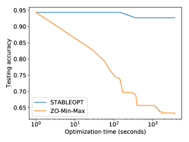
(c) (b) (c)

Figure 3: Empirical performance of ZO-Min-Max in design of poisoning attack: a) stationary gap versus iterations b) testing accuracy versus iterations (the shaded region represents variance of $10$ random trials), and c) comparison between ZO-Min-Max and STABLEOPT on testing accuracy versus optimization time.

In Figure 2, we compare the attack loss of using ZO-Min-Max with that of using ZO-PGD, which solves problem (6.1) by calling for an internal maximization oracle in $\mathbf{w}$ (see Appendix D). As we can see, ZO-Min-Max converges slower than ZO-PGD at early iterations. That is because the former only performs one-step PGA to update $\mathbf{w}$, while the latter solves the $\mathbf{w}$-maximization problem analytically. However, as the number of iterations increases, ZO-Min-Max achieves almost the same performance as ZO-PGD.

In Appendix D, we have provided additional comparisons on ZO-Min-Max versus ZO-Finite-Sum, and versus per-image PGD attack (Madry et al., 2018).

6.2 Black-box data poisoning attack

Data poisoning against logistic regression.

Let $\mathcal{D}=\{\mathbf{z}_{i},t_{i}\}_{i=1}^{n}$ denote the training dataset, among which $n^{\prime}\ll n$ samples are corrupted by a perturbation vector $\mathbf{x}$, leading to poisoned training data $\mathbf{z}_{i}+\mathbf{x}$ towards breaking the training process and thus the prediction accuracy. The poisoning attack problem is then formulated as

$$\displaystyle\operatorname*{\text{maximize}}_{\|\mathbf{x}\|_{\infty}\leq\epsilon}\operatorname*{\text{minimize}}_{\boldsymbol{\theta}}~{}g(\mathbf{x},\boldsymbol{\theta})\mathrel{\mathop{:}}=\{F_{\mathrm{tr}}(\mathbf{x},\boldsymbol{\theta};\mathcal{D}_{0})+\lambda\|\boldsymbol{\theta}\|_{2}^{2}\},$$ (17)

where $\mathbf{x}$ and $\boldsymbol{\theta}$ are optimization variables, $F_{\mathrm{tr}}(\mathbf{x},\boldsymbol{\theta};\mathcal{D}_{0})$ denotes the training loss over model parameters $\boldsymbol{\theta}$ at the presence of data poison $\mathbf{x}$, and $\lambda>0$ is a regularization parameter. Note that problem (17) can be written in the form of (2), $\min_{\mathbf{x}}\max_{\boldsymbol{\theta}}-g(\mathbf{x},\boldsymbol{\theta})$. Clearly, if $F_{\mathrm{tr}}$ is a convex loss, e.g., logistic regression or linear regression (Jagielski et al., 2018)), then $-g$ is strongly concave in $\boldsymbol{\theta}$. Since the adversary has no knowledge on the training objective and the benign training data, $g(\mathbf{x},\boldsymbol{\theta})$ is a two-sided black-box function in both $\mathbf{x}$ and $\boldsymbol{\theta}$ from the adversary’s perspective.

Implementation & Baseline.

In problem (17), we set the poisoning ratio $n^{\prime}/n=15\%$ and $\lambda=10^{-3}$ for problem (17), where the sensitivity of $\lambda$ is studied in Figure A4. More details on the specification of problem (17) are provided in Appendix E. In Algorithm A1, unless specified otherwise we choose $b=100$, $q=5$, $\alpha=0.02$, $\beta=0.05$, and $T=50000$. We report the empirical results averaged over $10$ independent trials with random initialization. We compare our method with FO-Min-Max and the state-of-the-art BO-based method STABLEOPT (Bogunovic et al., 2018).

In Figure 3, we present the convergence of ZO-Min-Max to generate data poisoning attack and validate the resulting attack performance in terms of testing accuracy of the logistic regression model trained on the poisoned dataset. Figure 3-(a) shows the stationary gap of ZO-Min-Max under different number of random direction vectors in gradient estimation (3). As we can see, a moderate choice of $q$ (e.g., $q\geq 5$ in our example) is sufficient to achieve near-optimal solution compared with FO-Min-Max. However, it suffers from a convergence bias, consistent with Theorem 2. Figure 3-(b) demonstrates the testing accuracy (against iterations) of the model learnt from poisoned training data, where the poisoning attack is generated by ZO-Min-Max (black-box attack) and FO-Min-Max (white-box attack). As we can see, ZO-Min-Max yields promising attacking performance comparable to FO-Min-Max. We can also see that by contrast with the testing accuracy of the clean model ($94\%$ without poison), the poisoning attack eventually reduces the testing accuracy (below $70\%$). Furthermore In Figure 3-(c), we compare ZO-Min-Max with STABLEOPT (Bogunovic et al., 2018) in terms of testing accuracy versus computation time, where the lower the accuracy is, the stronger the generated attack is. We observe that STABLEOPT has a poorer scalability while our method reaches a data poisoning attack that induces much lower testing accuracy within $500$ seconds. In Appendix E, we provide additional results on the model learnt under different data poisoning ratios.

7 Conclusion

This paper addresses black-box robust optimization problems given a finite number of function evaluations. In particular, we present ZO-Min-Max: a framework of alternating, randomized gradient estimation based ZO optimization algorithm to find a first-order stationary solution to the black-box min-max problem. Under mild assumptions, ZO-Min-Max enjoys a sub-linear convergence rate. It scales to dimensions that are infeasible for recent robust solvers based on Bayesian optimization. Furthermore, we experimentally demonstrate the potential application of the framework on generating black-box evasion and data poisoning attacks.

Appendix

Appendix A The ZO-Min-Max Algorithm

Algorithm A1 ZO-Min-Max to solve problem (2)

Input: given $\mathbf{x}^{(0)}$and $\mathbf{y}^{(0)}$, learning rates $\alpha$and $\beta$, the number of random directions $q$, and the possible mini-batch size $b$for stochastic optimization $t=1,2,\ldots,T$$\mathbf{x}$-step: perform ZO-PGD () $\mathbf{y}$-step: $f(\mathbf{x}^{(t)},\mathbf{y})$is black box w.r.t. $\mathbf{y}$perform ZO-PGA () perform PGA using $\nabla_{\mathbf{y}}f(\mathbf{x}^{(t)},\mathbf{y}^{(t-1)})$like ()

Appendix B Detailed Convergence Analysis

B.1 Table of Parameters

In Table A1, we summarize the problem and algorithmic parameters used in our convergence analysis.

Table A1: Summary of problem and algorithmic parameters and their descriptions.

parameter description $d$ # of optimization variables $b$ mini-batch size $q$ # of random direction vectors used in ZO gradient estimation $\alpha$ learning rate for ZO-PGD $\beta$ learning rate for ZO-PGA $\gamma$ strongly concavity parameter of $f(\mathbf{x},\mathbf{y})$ with respect to $\mathbf{y}$ $\eta$ upper bound on the gradient norm, implying Lipschitz continuity $L_{x}$, $L_{y}$ Lipschitz continuous gradient constant of $f(\mathbf{x},\mathbf{y})$ with respect to $\mathbf{x}$ and $\mathbf{y}$ respectively $R$ diameter of the compact convex set $\mathcal{X}$ or $\mathcal{Y}$ $f^{*}$ lower bound on the function value, implying feasibility $\sigma_{x}^{2}$, $\sigma_{y}^{2}$ variances of ZO gradient estimator for variables $\mathbf{x}$ and $\mathbf{y}$, bounded by (4)

B.2 Proof of Lemma 1

Before going into the proof, let’s review some preliminaries and give some definitions. Define $h_{\mu}(\operatorname{\mathbf{x}},\operatorname{\boldsymbol{\xi}})$ to be the smoothed version of $h(\operatorname{\mathbf{x}},\operatorname{\boldsymbol{\xi}})$ and since $\operatorname{\boldsymbol{\xi}}$ models a subsampling process over a finite number of candidate functions, we can further have $h_{\mu}(\operatorname{\mathbf{x}})\triangleq\mathbb{E}_{\operatorname{\boldsymbol{\xi}}}[h_{\mu}(\operatorname{\mathbf{x}},\boldsymbol{\xi})]$ and $\nabla_{\operatorname{\mathbf{x}}}h_{\mu}(\operatorname{\mathbf{x}})=\mathbb{E}_{\operatorname{\boldsymbol{\xi}}}[\nabla_{\mathbf{x}}h_{\mu}(\operatorname{\mathbf{x}},\boldsymbol{\xi})]$

Recall that in the finite sum setting when $\boldsymbol{\xi}_{j}$ parameterizes the $j$th function, the gradient estimator is given by

$$\widehat{\nabla}_{\mathbf{x}}h(\mathbf{x})={\frac{1}{bq}\sum_{j\in\mathcal{I}}\sum_{i=1}^{q}\frac{d[h(\mathbf{x}+\mu\mathbf{u}_{i};\boldsymbol{\xi}_{j})-h(\mathbf{x};\boldsymbol{\xi}_{j})]}{\mu}}\mathbf{u}_{i}.$$ (18)

where $\mathcal{I}$ is a set with $b$ elements, containing the indices of functions selected for gradient evaluation.

From standard result of the zeroth order gradient estimator, we know

$$\mathbb{E}_{\mathcal{I}}\left[\mathbb{E}_{\mathbf{u}_{i},i\in[q]}\left[\widehat{\nabla}_{\mathbf{x}}h(\mathbf{x})\right]\big{|}\mathcal{I}\right]=\mathbb{E}_{\mathcal{I}}\left[\frac{1}{b}\sum_{j\in\mathcal{I}}\nabla_{\operatorname{\mathbf{x}}}f_{\mu}(\operatorname{\mathbf{x}},\operatorname{\boldsymbol{\xi}}_{j})\right]=\nabla_{\operatorname{\mathbf{x}}}h_{\mu}(\operatorname{\mathbf{x}}).$$ (19)

Now let’s go into the proof. First, we have

$$\mathbb{E}\left[\|\widehat{\nabla}_{\mathbf{x}}h(\mathbf{x})-\nabla_{\mathbf{x}}h_{\mu}(\mathbf{x})\|_{2}^{2}\right]$$

$$= \mathbb{E}_{\mathcal{I}}\left[\mathbb{E}_{\mathbf{u}_{i},i\in[q]}\left[\left\|\widehat{\nabla}_{\mathbf{x}}h(\mathbf{x})-\frac{1}{b}\sum_{j\in\mathcal{I}}\nabla_{\operatorname{\mathbf{x}}}f_{\mu}(\operatorname{\mathbf{x}},\operatorname{\boldsymbol{\xi}}_{j})+\frac{1}{b}\sum_{j\in\mathcal{I}}\nabla_{\operatorname{\mathbf{x}}}f_{\mu}(\operatorname{\mathbf{x}},\operatorname{\boldsymbol{\xi}}_{j})-\nabla_{\mathbf{x}}h_{\mu}(\mathbf{x})\right\|_{2}^{2}\bigg{|}\mathcal{I}\right]\right]$$

$$\leq 2\mathbb{E}_{\mathcal{I}}\left[\mathbb{E}_{\mathbf{u}_{i},i\in[q]}\left[\left\|\widehat{\nabla}_{\mathbf{x}}h(\mathbf{x})-\frac{1}{b}\sum_{j\in\mathcal{I}}\nabla_{\operatorname{\mathbf{x}}}f_{\mu}(\operatorname{\mathbf{x}},\operatorname{\boldsymbol{\xi}}_{j})\right\|_{2}^{2}+\left\|\frac{1}{b}\sum_{j\in\mathcal{I}}\nabla_{\operatorname{\mathbf{x}}}f_{\mu}(\operatorname{\mathbf{x}},\operatorname{\boldsymbol{\xi}}_{j})-\nabla_{\mathbf{x}}h_{\mu}(\mathbf{x})\right\|_{2}^{2}\bigg{|}\mathcal{I}\right]\right].$$ (20)

Further, by definition, given $\mathcal{I}$, $\widehat{\nabla}_{\mathbf{x}}h(\mathbf{x})$ is the average of ZO gradient estimates under $q$ i.i.d. random directions, each of which has the mean $\frac{1}{b}\sum_{j\in\mathcal{I}}\nabla_{\operatorname{\mathbf{x}}}f_{\mu}(\operatorname{\mathbf{x}},\operatorname{\boldsymbol{\xi}}_{j})$.

Thus for the first term at the right-hand-side (RHS) of the above inequality, we have

$$\mathbb{E}_{\mathbf{u}_{i},i\in[q]}\left[\left\|\widehat{\nabla}_{\mathbf{x}}h(\mathbf{x})-\frac{1}{b}\sum_{j\in\mathcal{I}}\nabla_{\operatorname{\mathbf{x}}}f_{\mu}(\operatorname{\mathbf{x}},\operatorname{\boldsymbol{\xi}}_{j})\right\|_{2}^{2}\bigg{|}\mathcal{I}\right]\leq \frac{1}{q}\left(2d\left\|\frac{1}{b}\sum_{j\in\mathcal{I}}\nabla_{\operatorname{\mathbf{x}}}f(\operatorname{\mathbf{x}},\operatorname{\boldsymbol{\xi}}_{j})\right\|^{2}+\frac{\mu^{2}L_{h}^{2}d^{2}}{2}\right)$$

$$\leq \frac{1}{q}\left(2d\eta^{2}+\frac{\mu^{2}L_{h}^{2}d^{2}}{2}\right)$$ (21)

where the first inequality is by the standard bound of the variance of zeroth order estimator and the second inequality is by the assumption that $\|\nabla_{\operatorname{\mathbf{x}}}h(x;\boldsymbol{\xi})\|^{2}\leq\eta^{2}$ and thus $\|\frac{1}{b}\sum_{j\in\mathcal{I}}\nabla_{\operatorname{\mathbf{x}}}f(\operatorname{\mathbf{x}},\operatorname{\boldsymbol{\xi}}_{j})\|^{2}\leq\eta^{2}$.

In addition, we have

$$\mathbb{E}_{\mathcal{I}}\left[\mathbb{E}_{\mathbf{u}_{i},i\in[q]}\left[\left\|\frac{1}{b}\sum_{j\in\mathcal{I}}\nabla_{\operatorname{\mathbf{x}}}f_{\mu}(\operatorname{\mathbf{x}},\operatorname{\boldsymbol{\xi}}_{j})-\nabla_{\mathbf{x}}h_{\mu}(\mathbf{x})\right\|_{2}^{2}\bigg{|}\mathcal{I}\right]\right]$$

$$= \mathbb{E}_{\mathcal{I}}\left[\left\|\frac{1}{b}\sum_{j\in\mathcal{I}}\nabla_{\operatorname{\mathbf{x}}}f_{\mu}(\operatorname{\mathbf{x}},\operatorname{\boldsymbol{\xi}}_{j})-\nabla_{\mathbf{x}}h_{\mu}(\mathbf{x})\right\|_{2}^{2}\right]$$

$$= \frac{1}{b}\mathbb{E}_{\xi}\left[\left\|\nabla_{\operatorname{\mathbf{x}}}f_{\mu}(\operatorname{\mathbf{x}},\operatorname{\boldsymbol{\xi}})-\nabla_{\mathbf{x}}h_{\mu}(\mathbf{x})\right\|_{2}^{2}\right]\leq\frac{\eta^{2}}{b}$$ (22)

where the second equality is because $\xi_{j}$ are i.i.d. draws from the same distribution as $\xi$ and $\mathbb{E}[\nabla_{\operatorname{\mathbf{x}}}f_{\mu}(\operatorname{\mathbf{x}},\operatorname{\boldsymbol{\xi}})]=\nabla_{\mathbf{x}}h_{\mu}(\mathbf{x})$, the last inequality is because $\|\nabla_{\operatorname{\mathbf{x}}}f_{\mu}(\operatorname{\mathbf{x}},\operatorname{\boldsymbol{\xi}})\|_{2}^{2}\leq\eta^{2}$ by assumption. Substituting (B.2) and (B.2) into (B.2) finishes the proof. $\square$

B.3 Convergence Analysis of ZO-Min-Max by Performing PGA

In this section, we will provide the details of the proofs. Before proceeding, we have the following illustration, which will be useful in the proof.

The order of taking expectation:

Since iterates $\operatorname{\mathbf{x}}^{(t)},\operatorname{\mathbf{y}}^{(t)},\forall t$ are random variables, we need to define

$$\mathcal{F}^{(t)}=\{\operatorname{\mathbf{x}}^{(t)},\operatorname{\mathbf{y}}^{(t)},\operatorname{\mathbf{x}}^{(t-1)},\operatorname{\mathbf{y}}^{(t-1)},\ldots,\operatorname{\mathbf{x}}^{(1)},\operatorname{\mathbf{y}}^{(1)}\}$$ (23)

as the history of the iterates. Throughout the theoretical analysis, taking expectation means that we take expectation over random variable at the $t$th iteration conditioned on $\mathcal{F}^{(t-1)}$ and then take expectation over $\mathcal{F}^{(t-1)}$.

Subproblem:

Also, it is worthy noting that performing (5) and (6) are equivalent to the following optimization problem:

$$\operatorname{\mathbf{x}}^{(t)}= \min_{\operatorname{\mathbf{x}}\in\mathcal{X}}\left\langle\widehat{\nabla}_{\operatorname{\mathbf{x}}}f(\operatorname{\mathbf{x}}^{(t-1)},\operatorname{\mathbf{y}}^{(t-1)}),\operatorname{\mathbf{x}}-\operatorname{\mathbf{x}}^{(t-1)}\right\rangle+\frac{1}{2\alpha}\|\operatorname{\mathbf{x}}-\operatorname{\mathbf{x}}^{(t-1)}\|^{2},$$ (24)

$$\operatorname{\mathbf{y}}^{(t)}= \max_{\operatorname{\mathbf{y}}\in\mathcal{Y}}\left\langle\widehat{\nabla}_{\operatorname{\mathbf{y}}}f(\operatorname{\mathbf{x}}^{(t)},\operatorname{\mathbf{y}}^{(t-1)}),\operatorname{\mathbf{y}}-\operatorname{\mathbf{y}}^{(t-1)}\right\rangle-\frac{1}{2\beta}\|\operatorname{\mathbf{y}}-\operatorname{\mathbf{y}}^{(t-1)}\|^{2}.$$ (25)

When $f(\operatorname{\mathbf{x}},\operatorname{\mathbf{y}})$ is white-box w.r.t. $\mathbf{y}$, (25) becomes

$$\operatorname{\mathbf{y}}^{(t)}=\max_{\operatorname{\mathbf{y}}\in\mathcal{Y}}\left\langle{\nabla}_{\operatorname{\mathbf{y}}}f(\operatorname{\mathbf{x}}^{(t)},\operatorname{\mathbf{y}}^{(t-1)}),\operatorname{\mathbf{y}}-\operatorname{\mathbf{y}}^{(t-1)}\right\rangle-\frac{1}{2\beta}\|\operatorname{\mathbf{y}}-\operatorname{\mathbf{y}}^{(t-1)}\|^{2}.$$ (26)

In the proof of ZO-Min-Max, we will use the optimality condition of these two problems to derive the descent lemmas.

Relationship with smoothing function

We denote by $f_{\mu,x}(\mathbf{x},\mathbf{y})$ the smoothing version of $f$ w.r.t. $\mathbf{x}$ with parameter $\mu>0$. The similar definition holds for $f_{\mu,y}(\mathbf{x},\mathbf{y})$. By taking $f_{\mu,x}(\mathbf{x},\mathbf{y})$ as an example, under A2 $f$ and $f_{\mu,x}$ has the following relationship ([)Lemma 4.1]gao2014information:

$$|{f}_{\mu,\operatorname{\mathbf{x}}}(\operatorname{\mathbf{x}},\operatorname{\mathbf{y}})-f(\operatorname{\mathbf{x}},\operatorname{\mathbf{y}}))|\leq\frac{L_{x}\mu^{2}}{2}\quad\textrm{and}\quad\|\nabla_{\operatorname{\mathbf{x}}}{f}_{\mu,\operatorname{\mathbf{x}}}(\operatorname{\mathbf{x}},\operatorname{\mathbf{y}})-\nabla_{\operatorname{\mathbf{x}}}{f}(\operatorname{\mathbf{x}},\operatorname{\mathbf{y}})\|_{2}^{2}\leq\frac{\mu^{2}d^{2}L_{x}^{2}}{4},$$ (27)

$$|{f}_{\mu,\operatorname{\mathbf{y}}}(\operatorname{\mathbf{x}},\operatorname{\mathbf{y}})-f(\operatorname{\mathbf{x}},\operatorname{\mathbf{y}}))|\leq\frac{L_{y}\mu^{2}}{2}\quad\textrm{and}\quad\|\nabla_{\operatorname{\mathbf{y}}}{f}_{\mu,\operatorname{\mathbf{y}}}(\operatorname{\mathbf{x}},\operatorname{\mathbf{y}})-\nabla_{\operatorname{\mathbf{y}}}{f}(\operatorname{\mathbf{x}},\operatorname{\mathbf{y}})\|_{2}^{2}\leq\frac{\mu^{2}d^{2}L_{y}^{2}}{4}.$$ (28)

First, we will show the descent lemma in minimization as follows.

B.3.1 Proof of Lemma 2

Proof: Since $f(\mathbf{x},\mathbf{y})$ has $L_{x}$ Lipschtiz continuous gradients with respect to $\mathbf{x}$, we have

$$f_{\mu}(\operatorname{\mathbf{x}}^{(t+1)},\operatorname{\mathbf{y}}^{(t)})\leq f_{\mu}(\operatorname{\mathbf{x}}^{(t)},\operatorname{\mathbf{y}}^{(t)})+\langle\nabla_{\operatorname{\mathbf{x}}}f_{\mu}(\operatorname{\mathbf{x}}^{(t)},\operatorname{\mathbf{y}}^{(t)}),\operatorname{\mathbf{x}}^{(t+1)}-\operatorname{\mathbf{x}}^{(t)}\rangle+\frac{L_{x}}{2}\|\operatorname{\mathbf{x}}^{(t+1)}-\operatorname{\mathbf{x}}^{(t)}\|^{2}$$

$$= f_{\mu}(\operatorname{\mathbf{x}}^{(t)},\operatorname{\mathbf{y}}^{(t)})+\langle\widehat{\nabla}_{\operatorname{\mathbf{x}}}{f}(\operatorname{\mathbf{x}}^{(t)},\operatorname{\mathbf{y}}^{(t)}),\operatorname{\mathbf{x}}^{(t+1)}-\operatorname{\mathbf{x}}^{(t)}\rangle+\frac{L_{x}}{2}\|\operatorname{\mathbf{x}}^{(t+1)}-\operatorname{\mathbf{x}}^{(t)}\|^{2}$$

$$+\langle{\nabla}_{\operatorname{\mathbf{x}}}f_{\mu}(\operatorname{\mathbf{x}}^{(t)},\operatorname{\mathbf{y}}^{(t)})-\widehat{\nabla}_{\operatorname{\mathbf{x}}}{f}(\operatorname{\mathbf{x}}^{(t)},\operatorname{\mathbf{y}}^{(t)}),\operatorname{\mathbf{x}}^{(t+1)}-\operatorname{\mathbf{x}}^{(t)}\rangle.$$ (29)

Recall that

$$\mathbf{x}^{(t+1)}=\mathrm{proj}_{\mathcal{X}}(\mathbf{x}^{(t)}-\alpha\widehat{\nabla}_{\mathbf{x}}f(\mathbf{x}^{(t)},\mathbf{y}^{(t)})),$$ (30)

From the optimality condition of $\operatorname{\mathbf{x}}$-subproblem (24), we have

$$\langle\widehat{\nabla}_{\mathbf{x}}f(\mathbf{x}^{(t)},\operatorname{\mathbf{y}}^{(t)}),\operatorname{\mathbf{x}}^{(t+1)}-\operatorname{\mathbf{x}}^{(t)}\rangle\leq-\frac{1}{\alpha}\|\operatorname{\mathbf{x}}^{(t+1)}-\operatorname{\mathbf{x}}^{(t)}\|^{2}.$$ (31)

Here we use the fact that the optimality condition of problem (24) at the solution $\operatorname{\mathbf{x}}^{(t+1)}$ yields $\langle{\widehat{\nabla}_{\operatorname{\mathbf{x}}}f(\operatorname{\mathbf{x}}^{(t)},\operatorname{\mathbf{y}}^{(t)})+(\operatorname{\mathbf{x}}^{(t+1)}-\operatorname{\mathbf{x}}^{(t)})/\alpha,\operatorname{\mathbf{x}}^{(t+1)}-\mathbf{x}}\rangle\leq 0$ for any $\mathbf{x}\in\mathcal{X}$. By setting $\mathbf{x}=\mathbf{x}^{(t)}$, we obtain (31).

In addition, we define another iterate generated by $\nabla_{\operatorname{\mathbf{x}}}f_{\mu}(\operatorname{\mathbf{x}}^{(t)},\operatorname{\mathbf{y}}^{(t)})$

$$\mathbf{\widehat{x}}^{(t+1)}=\mathrm{proj}_{\mathcal{X}}(\mathbf{x}^{(t)}-\alpha{\nabla}_{\mathbf{x}}f_{\mu}(\mathbf{x}^{(t)},\mathbf{y}^{(t)})).$$ (32)

Then, we can have

$$\langle{\nabla}_{\operatorname{\mathbf{x}}}f_{\mu}(\operatorname{\mathbf{x}}^{(t)},\operatorname{\mathbf{y}}^{(t)})-\widehat{\nabla}_{\operatorname{\mathbf{x}}}{f}(\operatorname{\mathbf{x}}^{(t)},\operatorname{\mathbf{y}}^{(t)}),\operatorname{\mathbf{x}}^{(t+1)}-\operatorname{\mathbf{x}}^{(t)}\rangle$$

$$= \langle{\nabla}_{\operatorname{\mathbf{x}}}f_{\mu}(\operatorname{\mathbf{x}}^{(t)},\operatorname{\mathbf{y}}^{(t)})-\widehat{\nabla}_{\operatorname{\mathbf{x}}}{f}(\operatorname{\mathbf{x}}^{(t)},\operatorname{\mathbf{y}}^{(t)}),\operatorname{\mathbf{x}}^{(t+1)}-\operatorname{\mathbf{x}}^{(t)}-(\mathbf{\widehat{x}}^{(t+1)}-\operatorname{\mathbf{x}}^{(t)})\rangle$$

$$+\langle{\nabla}_{\operatorname{\mathbf{x}}}f_{\mu}(\operatorname{\mathbf{x}}^{(t)},\operatorname{\mathbf{y}}^{(t)})-\widehat{\nabla}_{\operatorname{\mathbf{x}}}{f}(\operatorname{\mathbf{x}}^{(t)},\operatorname{\mathbf{y}}^{(t)}),\mathbf{\widehat{x}}^{(t+1)}-\operatorname{\mathbf{x}}^{(t)}\rangle.$$ (33)

Due to the fact that $\mathbb{E}_{\mathbf{u}}[\widehat{\nabla}_{\operatorname{\mathbf{x}}}{f}(\operatorname{\mathbf{x}}^{(t)},\operatorname{\mathbf{y}}^{(t)})]=\nabla_{\operatorname{\mathbf{x}}}f_{\mu}(\operatorname{\mathbf{x}}^{(t)},\operatorname{\mathbf{y}}^{(t)}),$ we further have

$$\mathbb{E}_{\mathbf{u}}[\langle{\nabla}_{\operatorname{\mathbf{x}}}f_{\mu}(\operatorname{\mathbf{x}}^{(t)},\operatorname{\mathbf{y}}^{(t)})-\widehat{\nabla}_{\operatorname{\mathbf{x}}}{f}(\operatorname{\mathbf{x}}^{(t)},\operatorname{\mathbf{y}}^{(t)}),\mathbf{\widehat{x}}^{(t+1)}-\operatorname{\mathbf{x}}^{(t)}\rangle]=0.$$ (34)

Finally, we also have

$$\langle{\nabla}_{\operatorname{\mathbf{x}}}f_{\mu}(\operatorname{\mathbf{x}}^{(t)},\operatorname{\mathbf{y}}^{(t)})-\widehat{\nabla}_{\operatorname{\mathbf{x}}}{f}(\operatorname{\mathbf{x}}^{(t)},\operatorname{\mathbf{y}}^{(t)}),\operatorname{\mathbf{x}}^{(t+1)}-\operatorname{\mathbf{x}}^{(t)}-(\mathbf{\widehat{x}}^{(t+1)}-\operatorname{\mathbf{x}}^{(t)})\rangle$$

$$\leq \frac{\alpha}{2}\|{\nabla}_{\operatorname{\mathbf{x}}}f_{\mu}(\operatorname{\mathbf{x}}^{(t)},\operatorname{\mathbf{y}}^{(t)})-\widehat{\nabla}_{\operatorname{\mathbf{x}}}{f}(\operatorname{\mathbf{x}}^{(t)},\operatorname{\mathbf{y}}^{(t)})\|^{2}+\frac{1}{2\alpha}\|\operatorname{\mathbf{x}}^{(t+1)}-\operatorname{\mathbf{x}}^{(t)}-(\mathbf{\widehat{x}}^{(t+1)}-\operatorname{\mathbf{x}}^{(t)})\|^{2}$$

$$\leq \alpha\|{\nabla}_{\operatorname{\mathbf{x}}}f_{\mu}(\operatorname{\mathbf{x}}^{(t)},\operatorname{\mathbf{y}}^{(t)})-\widehat{\nabla}_{\operatorname{\mathbf{x}}}{f}(\operatorname{\mathbf{x}}^{(t)},\operatorname{\mathbf{y}}^{(t)})\|^{2}$$ (35)

where the first inequality is due to Young’s inequality, the second inequality is due to non-expansiveness of the projection operator. Thus

$$\mathbb{E}_{\mathbf{u}}[\langle{\nabla}_{\operatorname{\mathbf{x}}}f_{\mu}(\operatorname{\mathbf{x}}^{(t)},\operatorname{\mathbf{y}}^{(t)})-\widehat{\nabla}_{\operatorname{\mathbf{x}}}{f}(\operatorname{\mathbf{x}}^{(t)},\operatorname{\mathbf{y}}^{(t)}),\operatorname{\mathbf{x}}^{(t+1)}-\operatorname{\mathbf{x}}^{(t)}-(\mathbf{\widehat{x}}^{(t+1)}-\operatorname{\mathbf{x}}^{(t)})\rangle]$$

$$\leq \mathbb{E}_{\mathbf{u}}[\alpha\|{\nabla}_{\operatorname{\mathbf{x}}}f_{\mu}(\operatorname{\mathbf{x}}^{(t)},\operatorname{\mathbf{y}}^{(t)})-\widehat{\nabla}_{\operatorname{\mathbf{x}}}{f}(\operatorname{\mathbf{x}}^{(t)},\operatorname{\mathbf{y}}^{(t)})\|^{2}]\leq\alpha\sigma_{x}^{2}$$ (36)

where $\sigma_{x}^{2}\mathrel{\mathop{:}}=\sigma^{2}(L_{x},b,q,d)$ which was defined in (4).

Combining all above, we have

$$\mathbb{E}[f_{\mu}(\operatorname{\mathbf{x}}^{(t+1)},\operatorname{\mathbf{y}}^{(t)})]\leq \mathbb{E}[f_{\mu}(\operatorname{\mathbf{x}}^{(t)},\operatorname{\mathbf{y}}^{(t)})]-\left(\frac{1}{\alpha}-\frac{L_{x}}{2}\right)\|\operatorname{\mathbf{x}}^{(t+1)}-\operatorname{\mathbf{x}}^{(t)}\|^{2}+\alpha\sigma^{2},$$ (37)

and we request $\alpha\leq 1/L_{x}$, which completes the proof.

Using $|{f}_{\mu,x}(\operatorname{\mathbf{x}},\operatorname{\mathbf{y}})-f(\operatorname{\mathbf{x}},\operatorname{\mathbf{y}}))|\leq\frac{L_{x}\mu^{2}}{2}$, we can get

$$\mathbb{E}[f(\operatorname{\mathbf{x}}^{(t+1)},\operatorname{\mathbf{y}}^{(t)})]-\frac{L_{x}\mu^{2}}{2}\leq\mathbb{E}[f_{\mu}(\operatorname{\mathbf{x}}^{(t+1)},\operatorname{\mathbf{y}}^{(t)})]\leq\mathbb{E}[f(\operatorname{\mathbf{x}}^{(t+1)},\operatorname{\mathbf{y}}^{(t)})]+\frac{L_{x}\mu^{2}}{2},$$ (38)

so we are able to obtain from (4)

$$\mathbb{E}[f(\operatorname{\mathbf{x}}^{(t+1)},\operatorname{\mathbf{y}}^{(t)})]\leq\mathbb{E}[f(\operatorname{\mathbf{x}}^{(t)},\operatorname{\mathbf{y}}^{(t)})]-\left(\frac{1}{\alpha}-\frac{L_{x}}{2}\right)\|\operatorname{\mathbf{x}}^{(t+1)}-\operatorname{\mathbf{x}}^{(t)}\|^{2}+\alpha\sigma^{2}_{x}+L_{x}\mu^{2}.$$ (39)

$\square$

Corollary 1.

$$\mathbb{E}\left\langle\widehat{\nabla}f(\operatorname{\mathbf{x}}^{(t)},\operatorname{\mathbf{y}}^{(t-1)})-\nabla f_{\mu}(\operatorname{\mathbf{x}}^{(t)},\operatorname{\mathbf{y}}^{(t-1)}),\operatorname{\mathbf{y}}^{(t)}-\operatorname{\mathbf{y}}^{(t-1)}\right\rangle\leq\beta\sigma_{y}^{2}$$ (40)

$\sigma_{y}^{2}\mathrel{\mathop{:}}=\sigma^{2}(L_{y},b,q,d)$ which was defined in (4).

Proof:

Define

$$\mathbf{\widetilde{y}}^{(t)}=\mathrm{proj}_{\mathcal{Y}}(\mathbf{y}^{(t)}-\beta{\nabla}_{\mathbf{y}}f_{\mu}(\mathbf{x}^{(t)},\mathbf{y}^{(t-1)})),$$ (41)

we have

$$\langle{\nabla}_{\operatorname{\mathbf{y}}}f_{\mu}(\operatorname{\mathbf{x}}^{(t)},\operatorname{\mathbf{y}}^{(t-1)})-\widehat{\nabla}_{\operatorname{\mathbf{x}}}{f}(\operatorname{\mathbf{x}}^{(t)},\operatorname{\mathbf{y}}^{(t-1)}),\operatorname{\mathbf{y}}^{(t)}-\operatorname{\mathbf{y}}^{(t-1)}\rangle$$

$$= \langle{\nabla}_{\operatorname{\mathbf{y}}}f_{\mu}(\operatorname{\mathbf{x}}^{(t)},\operatorname{\mathbf{y}}^{(t-1)})-\widehat{\nabla}_{\operatorname{\mathbf{y}}}{f}(\operatorname{\mathbf{x}}^{(t)},\operatorname{\mathbf{y}}^{(t-1)}),\operatorname{\mathbf{y}}^{(t)}-\operatorname{\mathbf{y}}^{(t-1)}-(\mathbf{\widetilde{y}}^{(t)}-\operatorname{\mathbf{y}}^{(t-1)})\rangle$$

$$+\langle{\nabla}_{\operatorname{\mathbf{y}}}f_{\mu}(\operatorname{\mathbf{x}}^{(t)},\operatorname{\mathbf{y}}^{(t-1)})-\widehat{\nabla}_{\operatorname{\mathbf{y}}}{f}(\operatorname{\mathbf{x}}^{(t)},\operatorname{\mathbf{y}}^{(t-1)}),\mathbf{\widetilde{y}}^{(t)}-\operatorname{\mathbf{y}}^{(t-1)}\rangle.$$ (42)

Due to the fact that $\mathbb{E}_{\mathbf{u}}[\widehat{\nabla}_{\operatorname{\mathbf{y}}}{f}(\operatorname{\mathbf{x}}^{(t)},\operatorname{\mathbf{y}}^{(t-1)})]=\nabla_{\operatorname{\mathbf{y}}}f_{\mu}(\operatorname{\mathbf{x}}^{(t)},\operatorname{\mathbf{y}}^{(t-1)}),$ we further have

$$\mathbb{E}_{\mathbf{u}}[\langle{\nabla}_{\operatorname{\mathbf{y}}}f_{\mu}(\operatorname{\mathbf{x}}^{(t)},\operatorname{\mathbf{y}}^{(t-1)})-\widehat{\nabla}_{\operatorname{\mathbf{y}}}{f}(\operatorname{\mathbf{x}}^{(t)},\operatorname{\mathbf{y}}^{(t-1)}),\mathbf{\widetilde{y}}^{(t)}-\operatorname{\mathbf{y}}^{(t-1)}\rangle]=0.$$ (43)

Finally, we also have

$$\mathbb{E}_{\mathbf{u}}[\langle{\nabla}_{\operatorname{\mathbf{y}}}f_{\mu}(\operatorname{\mathbf{x}}^{(t)},\operatorname{\mathbf{y}}^{(t-1)})-\widehat{\nabla}_{\operatorname{\mathbf{y}}}{f}(\operatorname{\mathbf{x}}^{(t)},\operatorname{\mathbf{y}}^{(t-1)}),\operatorname{\mathbf{y}}^{(t)}-\operatorname{\mathbf{y}}^{(t-1)}-(\mathbf{\widetilde{y}}^{(t)}-\operatorname{\mathbf{y}}^{(t-1)})\rangle]$$

$$\leq \mathbb{E}_{\mathbf{u}}[\frac{\beta}{2}\|\langle{\nabla}_{\operatorname{\mathbf{y}}}f_{\mu}(\operatorname{\mathbf{x}}^{(t)},\operatorname{\mathbf{y}}^{(t-1)})-\widehat{\nabla}_{\operatorname{\mathbf{y}}}{f}(\operatorname{\mathbf{x}}^{(t)},\operatorname{\mathbf{y}}^{(t-1)})\|^{2}+\frac{1}{2\beta}\|\operatorname{\mathbf{y}}^{(t)}-\operatorname{\mathbf{y}}^{(t-1)}-(\mathbf{\widetilde{y}}^{(t)}-\operatorname{\mathbf{y}}^{(t-1)})\|^{2}]$$

$$\leq \mathbb{E}_{\mathbf{u}}[\beta\|{\nabla}_{\operatorname{\mathbf{y}}}f_{\mu}(\operatorname{\mathbf{x}}^{(t)},\operatorname{\mathbf{y}}^{(t-1)})-\widehat{\nabla}_{\operatorname{\mathbf{y}}}{f}(\operatorname{\mathbf{x}}^{(t)},\operatorname{\mathbf{y}}^{(t-1)})\|^{2}]\leq\beta\sigma_{y}^{2}$$ (44)

where $\sigma_{y}^{2}\mathrel{\mathop{:}}=\sigma^{2}(L_{y},b,q,d)$ which was defined in (4).

$\square$

Next, before showing the proof of Lemma 3, we need the following lemma to show the recurrence of the size of the successive difference between two iterations.

Lemma 5.

Under assumption 1, assume iterates $\operatorname{\mathbf{x}}^{(t)},\operatorname{\mathbf{y}}^{(t)}$ generated by algorithm A1. When $f(\operatorname{\mathbf{x}}^{(t)},\operatorname{\mathbf{y}})$ is white-box, we have

$$\frac{2}{\beta^{2}\gamma}\mathbb{E}\|\operatorname{\mathbf{y}}^{(t+1)}-\operatorname{\mathbf{y}}^{(t)}\|^{2}-\frac{2}{\beta^{2}\gamma}\mathbb{E}\|\operatorname{\mathbf{y}}^{(t)}-\operatorname{\mathbf{y}}^{(t-1)}\|^{2}\leq\frac{2L^{2}_{x}}{\beta\gamma^{2}}\mathbb{E}\|\operatorname{\mathbf{x}}^{(t+1)}-\operatorname{\mathbf{x}}^{(t)}\|^{2}\\ +\frac{2}{\beta}\mathbb{E}\|\operatorname{\mathbf{y}}^{(t+1)}-\operatorname{\mathbf{y}}^{(t)}\|^{2}-\left(\frac{4}{\beta}-\frac{2L^{2}_{y}}{\gamma}\right)\mathbb{E}\|\operatorname{\mathbf{y}}^{(t)}-\operatorname{\mathbf{y}}^{(t-1)}\|^{2}.$$ (45)

Proof: from the optimality condition of $\operatorname{\mathbf{y}}$-subproblem (26) at iteration $t$ and $t-1$, we have the following two inequalities:

$$-\langle\nabla_{\operatorname{\mathbf{y}}}f(\operatorname{\mathbf{x}}^{(t+1)},\operatorname{\mathbf{y}}^{(t)})-\frac{1}{\beta}(\operatorname{\mathbf{y}}^{(t+1)}-\operatorname{\mathbf{y}}^{(t)}),\operatorname{\mathbf{y}}^{(t+1)}-\operatorname{\mathbf{y}}^{(t)}\rangle\leq 0,$$ (46)

$$\langle\nabla_{\operatorname{\mathbf{y}}}f(\operatorname{\mathbf{x}}^{(t)},\operatorname{\mathbf{y}}^{(t-1)})-\frac{1}{\beta}(\operatorname{\mathbf{y}}^{(t)}-\operatorname{\mathbf{y}}^{(t-1)}),\operatorname{\mathbf{y}}^{(t+1)}-\operatorname{\mathbf{y}}^{(t)}\rangle\leq 0.$$ (47)

Adding the above inequalities, we can get

$$\frac{1}{\beta}\langle\operatorname{\mathbf{v}}^{(t+1)},\operatorname{\mathbf{y}}^{(t+1)}-\operatorname{\mathbf{y}}^{(t)}\rangle\leq\left\langle\nabla_{\operatorname{\mathbf{y}}}f(\operatorname{\mathbf{x}}^{(t+1)},\operatorname{\mathbf{y}}^{(t)})-\nabla_{\operatorname{\mathbf{y}}}f(\operatorname{\mathbf{x}}^{(t)},\operatorname{\mathbf{y}}^{(t)}),\operatorname{\mathbf{y}}^{(t+1)}-\operatorname{\mathbf{y}}^{(t)}\right\rangle$$

$$+\left\langle\nabla_{\operatorname{\mathbf{y}}}f(\operatorname{\mathbf{x}}^{(t)},\operatorname{\mathbf{y}}^{(t)})-\nabla_{\operatorname{\mathbf{y}}}f(\operatorname{\mathbf{x}}^{(t)},\operatorname{\mathbf{y}}^{(t-1)}),\operatorname{\mathbf{y}}^{(t+1)}-\operatorname{\mathbf{y}}^{(t)}\right\rangle$$ (48)

where $\operatorname{\mathbf{v}}^{(t+1)}=\operatorname{\mathbf{y}}^{(t+1)}-\operatorname{\mathbf{y}}^{(t)}-(\operatorname{\mathbf{y}}^{(t)}-\operatorname{\mathbf{y}}^{(t-1)})$.

According to the quadrilateral indentity, we know

$$\left\langle\operatorname{\mathbf{v}}^{(t+1)},\operatorname{\mathbf{y}}^{(t+1)}-\operatorname{\mathbf{y}}^{(t)}\right\rangle=\frac{1}{2}\left(\|\operatorname{\mathbf{y}}^{(t+1)}-\operatorname{\mathbf{y}}^{(t)}\|^{2}+\|\operatorname{\mathbf{v}}^{(t+1)}\|^{2}-\|\operatorname{\mathbf{y}}^{(t)}-\operatorname{\mathbf{y}}^{(t-1)}\|^{2}\right).$$ (49)

Based on the definition of $\mathbf{v}^{(t+1)}$, we substituting (49) into (48), which gives

$$\frac{1}{2\beta}\|\operatorname{\mathbf{y}}^{(t+1)}-\operatorname{\mathbf{y}}^{(t)}\|^{2}\leq \frac{1}{2\beta}\|\operatorname{\mathbf{y}}^{(t)}-\operatorname{\mathbf{y}}^{(t-1)}\|^{2}-\frac{1}{2\beta}\|\operatorname{\mathbf{v}}^{(t+1)}\|^{2}$$

$$+\left\langle\nabla_{\operatorname{\mathbf{y}}}f(\operatorname{\mathbf{x}}^{(t+1)},\operatorname{\mathbf{y}}^{(t)})-\nabla_{\operatorname{\mathbf{y}}}f(\operatorname{\mathbf{x}}^{(t)},\operatorname{\mathbf{y}}^{(t)}),\operatorname{\mathbf{y}}^{(t+1)}-\operatorname{\mathbf{y}}^{(t)}\right\rangle$$

$$+\left\langle\nabla_{\operatorname{\mathbf{y}}}f(\operatorname{\mathbf{x}}^{(t)},\operatorname{\mathbf{y}}^{(t)})-\nabla_{\operatorname{\mathbf{y}}}f(\operatorname{\mathbf{x}}^{(t)},\operatorname{\mathbf{y}}^{(t-1)}),\operatorname{\mathbf{y}}^{(t+1)}-\operatorname{\mathbf{y}}^{(t)}\right\rangle$$ (50)

$$\mathop{\leq}\limits^{(a)} \frac{1}{2\beta}\|\operatorname{\mathbf{y}}^{(t)}-\operatorname{\mathbf{y}}^{(t-1)}\|^{2}+\left\langle\nabla_{\operatorname{\mathbf{y}}}f(\operatorname{\mathbf{x}}^{(t+1)},\operatorname{\mathbf{y}}^{(t)})-\nabla_{\operatorname{\mathbf{y}}}f(\operatorname{\mathbf{x}}^{(t)},\operatorname{\mathbf{y}}^{(t)}),\operatorname{\mathbf{y}}^{(t+1)}-\operatorname{\mathbf{y}}^{(t)}\right\rangle$$

$$+\frac{\beta L^{2}_{y}}{2}\|\operatorname{\mathbf{y}}^{(t)}-\operatorname{\mathbf{y}}^{(t-1)}\|^{2}-\gamma\|\operatorname{\mathbf{y}}^{(t)}-\operatorname{\mathbf{y}}^{(t-1)}\|^{2}$$

$$\mathop{\leq}\limits^{(b)} \frac{1}{2\beta}\|\operatorname{\mathbf{y}}^{(t)}-\operatorname{\mathbf{y}}^{(t-1)}\|^{2}+\frac{\gamma}{2}\|\operatorname{\mathbf{y}}^{(t+1)}-\operatorname{\mathbf{y}}^{(t)}\|^{2}$$

$$+\frac{L^{2}_{x}}{2\gamma}\|\operatorname{\mathbf{x}}^{(t+1)}-\operatorname{\mathbf{x}}^{(t)}\|^{2}-(\gamma-\frac{\beta L^{2}_{y}}{2})\|\operatorname{\mathbf{y}}^{(t)}-\operatorname{\mathbf{y}}^{(t-1)}\|^{2}$$ (51)

where in $(a)$ we use the strong concavity of function $f(\operatorname{\mathbf{x}},\operatorname{\mathbf{y}})$ in $\operatorname{\mathbf{y}}$ (with parameter $\gamma>0$) and Young’s inequality, i.e.,

$$\langle\nabla_{\operatorname{\mathbf{y}}}f(\operatorname{\mathbf{x}}^{(t)},\operatorname{\mathbf{y}}^{(t)})-\nabla_{\operatorname{\mathbf{y}}}f(\operatorname{\mathbf{x}}^{(t)},\operatorname{\mathbf{y}}^{(t-1)}),\operatorname{\mathbf{y}}^{(t+1)}-\operatorname{\mathbf{y}}^{(t)}\rangle$$

$$= \langle\nabla_{\operatorname{\mathbf{y}}}f(\operatorname{\mathbf{x}}^{(t)},\operatorname{\mathbf{y}}^{(t)})-\nabla_{\operatorname{\mathbf{y}}}f(\operatorname{\mathbf{x}}^{(t)},\operatorname{\mathbf{y}}^{(t-1)}),\operatorname{\mathbf{v}}^{(t+1)}+\operatorname{\mathbf{y}}^{(t)}-\operatorname{\mathbf{y}}^{(t-1)}\rangle$$

$$\leq \frac{\beta L^{2}_{y}}{2}\|\operatorname{\mathbf{y}}^{(t)}-\operatorname{\mathbf{y}}^{(t-1)}\|^{2}+\frac{1}{2\beta}\|\operatorname{\mathbf{v}}^{(t+1)}\|^{2}-\gamma\|\operatorname{\mathbf{y}}^{(t)}-\operatorname{\mathbf{y}}^{(t-1)}\|^{2}$$ (52)

and in $(b)$ we apply the Young’s inequality, i.e.,

$$\left\langle\nabla_{\operatorname{\mathbf{y}}}f(\operatorname{\mathbf{x}}^{(t+1)},\operatorname{\mathbf{y}}^{(t)})-\nabla_{\operatorname{\mathbf{y}}}f(\operatorname{\mathbf{x}}^{(t)},\operatorname{\mathbf{y}}^{(t)}),\operatorname{\mathbf{y}}^{(t+1)}-\operatorname{\mathbf{y}}^{(t)}\right\rangle\leq\frac{L^{2}_{x}}{2\gamma}\|\operatorname{\mathbf{x}}^{(t+1)}-\operatorname{\mathbf{x}}^{(t)}\|^{2}+\frac{\gamma}{2}\|\operatorname{\mathbf{y}}^{(t+1)}-\operatorname{\mathbf{y}}^{(t)}\|^{2}.$$ (53)

Therefore, we have

$$\frac{1}{2\beta}\|\operatorname{\mathbf{y}}^{(t+1)}-\operatorname{\mathbf{y}}^{(t)}\|^{2}\leq \frac{1}{2\beta}\|\operatorname{\mathbf{y}}^{(t)}-\operatorname{\mathbf{y}}^{(t-1)}\|^{2}+\frac{L^{2}_{x}}{2\gamma}\|\operatorname{\mathbf{x}}^{(t+1)}-\operatorname{\mathbf{x}}^{(t)}\|^{2}$$

$$+\frac{\gamma}{2}\|\operatorname{\mathbf{y}}^{(t+1)}-\operatorname{\mathbf{y}}^{(t)}\|^{2}-\left(\gamma-\frac{\beta L^{2}_{y}}{2}\right)\|\operatorname{\mathbf{y}}^{(t)}-\operatorname{\mathbf{y}}^{(t-1)}\|^{2},$$ (54)

which implies

$$\frac{2}{\beta^{2}\gamma}\|\operatorname{\mathbf{y}}^{(t+1)}-\operatorname{\mathbf{y}}^{(t)}\|^{2}\leq \frac{2}{\beta^{2}\gamma}\|\operatorname{\mathbf{y}}^{(t)}-\operatorname{\mathbf{y}}^{(t-1)}\|^{2}+\frac{2L^{2}_{x}}{\beta\gamma^{2}}\|\operatorname{\mathbf{x}}^{(t+1)}-\operatorname{\mathbf{x}}^{(t)}\|^{2}$$

$$+\frac{2}{\beta}\|\operatorname{\mathbf{y}}^{(t+1)}-\operatorname{\mathbf{y}}^{(t)}\|^{2}-\left(\frac{4}{\beta}-\frac{2L^{2}_{y}}{\gamma}\right)\|\operatorname{\mathbf{y}}^{(t)}-\operatorname{\mathbf{y}}^{(t-1)}\|^{2}.$$ (55)

By taking the expectation on both sides of (55), we can get the results of Lemma 5. $\square$

Lemma 5 basically gives the recursion of $\|\Delta^{(t)}_{y}\|^{2}$. It can be observed that term $(4/\beta-2L^{2}_{y}/\gamma)\|\Delta^{(t)}_{\operatorname{\mathbf{y}}}\|$ provides the descent of the recursion when $\beta$ is small enough, which will take an important role in the proof of Lemma 3 when we quantify the descent in maximization.

Then, we can quantify the descent of the objective value by the following descent lemma.

B.3.2 Proof of Lemma 3

Proof: let $f^{\prime}(\operatorname{\mathbf{x}}^{(t+1)},\operatorname{\mathbf{y}}^{(t+1)})=f(\operatorname{\mathbf{x}}^{(t+1)},\operatorname{\mathbf{y}}^{(t+1)})-1(\operatorname{\mathbf{y}}^{(t+1)})$ and $1(\operatorname{\mathbf{y}})$ denote the indicator function with respect to the constraint of $\mathbf{y}$. From the optimality condition of sub-problem $\operatorname{\mathbf{y}}$ in (25), we have

$$\nabla_{\operatorname{\mathbf{y}}}f(\operatorname{\mathbf{x}}^{(t+1)},\operatorname{\mathbf{y}}^{(t)})-\frac{1}{\beta}(\operatorname{\mathbf{y}}^{(t+1)}-\operatorname{\mathbf{y}}^{(t)})-\xi^{(t+1)}=0$$ (56)

where $\xi^{(t)}$ denote the subgradient of $1(\operatorname{\mathbf{y}}^{(t)})$. Since function $f^{\prime}(\operatorname{\mathbf{x}},\operatorname{\mathbf{y}})$ is concave with respect to $\operatorname{\mathbf{y}}$, we have

$$f^{\prime}(\operatorname{\mathbf{x}}^{(t+1)},\operatorname{\mathbf{y}}^{(t+1)})-f^{\prime}(\operatorname{\mathbf{x}}^{(t+1)},\operatorname{\mathbf{y}}^{(t)})\leq\langle\nabla_{\operatorname{\mathbf{y}}}f(\operatorname{\mathbf{x}}^{(t+1)},\operatorname{\mathbf{y}}^{(t)}),\operatorname{\mathbf{y}}^{(t+1)}-\operatorname{\mathbf{y}}^{(t)}\rangle-\langle\xi^{(t)},\operatorname{\mathbf{y}}^{(t+1)}-\operatorname{\mathbf{y}}^{(t)}\rangle$$

$$\mathop{=}\limits^{(a)} \frac{1}{\beta}\|\operatorname{\mathbf{y}}^{(t+1)}-\operatorname{\mathbf{y}}^{(t)}\|^{2}-\langle\xi^{(t)}-\xi^{(t+1)},\operatorname{\mathbf{y}}^{(t+1)}-\operatorname{\mathbf{y}}^{(t)}\rangle$$

$$= \frac{1}{\beta}\|\operatorname{\mathbf{y}}^{(t+1)}-\operatorname{\mathbf{y}}^{(t)}\|^{2}+\left\langle\nabla_{\operatorname{\mathbf{y}}}f(\operatorname{\mathbf{x}}^{(t+1)},\operatorname{\mathbf{y}}^{(t)})-\nabla_{\operatorname{\mathbf{y}}}f(\operatorname{\mathbf{x}}^{(t)},\operatorname{\mathbf{y}}^{(t-1)}),\operatorname{\mathbf{y}}^{(t+1)}-\operatorname{\mathbf{y}}^{(t)}\right\rangle$$

$$-\frac{1}{\beta}\left\langle\operatorname{\mathbf{v}}^{(t+1)},\operatorname{\mathbf{y}}^{(t+1)}-\operatorname{\mathbf{y}}^{(t)}\right\rangle$$ (57)

where in $(a)$ we use $\xi^{(t+1)}=\nabla_{\operatorname{\mathbf{y}}}f(\operatorname{\mathbf{x}}^{(t+1)},\operatorname{\mathbf{y}}^{(t)})-\frac{1}{\beta}(\operatorname{\mathbf{y}}^{(t+1)}-\operatorname{\mathbf{y}}^{(t)})$ .

The last two terms of (57) is the same as the RHS of (48). We can apply the similar steps from (50) to (51). To be more specific, the derivations are shown as follows: First, we know

$$f^{\prime}(\operatorname{\mathbf{x}}^{(t+1)},\operatorname{\mathbf{y}}^{(t+1)})-f^{\prime}(\operatorname{\mathbf{x}}^{(t+1)},\operatorname{\mathbf{y}}^{(t)})\leq\frac{1}{\beta}\|\operatorname{\mathbf{y}}^{(t+1)}-\operatorname{\mathbf{y}}^{(t)}\|^{2}\\ +\left\langle\nabla_{\operatorname{\mathbf{y}}}f(\operatorname{\mathbf{x}}^{(t+1)},\operatorname{\mathbf{y}}^{(t)})-\nabla_{\operatorname{\mathbf{y}}}f(\operatorname{\mathbf{x}}^{(t)},\operatorname{\mathbf{y}}^{(t-1)}),\operatorname{\mathbf{y}}^{(t+1)}-\operatorname{\mathbf{y}}^{(t)}\right\rangle-\frac{1}{\beta}\left\langle\operatorname{\mathbf{v}}^{(t+1)},\operatorname{\mathbf{y}}^{(t+1)}-\operatorname{\mathbf{y}}^{(t)}\right\rangle.$$ (58)

Then, we move term $1/\beta\langle\operatorname{\mathbf{v}}^{(t+1)},\operatorname{\mathbf{y}}^{(t+1)}-\operatorname{\mathbf{y}}^{(t)}\rangle$ to RHS of (57) and have

$$f(\operatorname{\mathbf{x}}^{(t+1)},\operatorname{\mathbf{y}}^{(t+1)})-f(\operatorname{\mathbf{x}}^{(t+1)},\operatorname{\mathbf{y}}^{(t)})$$

$$\leq \frac{1}{2\beta}\|\operatorname{\mathbf{y}}^{(t+1)}-\operatorname{\mathbf{y}}^{(t)}\|^{2}+\frac{1}{2\beta}\|\operatorname{\mathbf{y}}^{(t)}-\operatorname{\mathbf{y}}^{(t-1)}\|^{2}-\frac{1}{2\beta}\|\operatorname{\mathbf{v}}^{(t+1)}\|^{2}$$

$$+\left\langle\nabla_{\operatorname{\mathbf{y}}}f(\operatorname{\mathbf{x}}^{(t+1)},\operatorname{\mathbf{y}}^{(t)})-\nabla_{\operatorname{\mathbf{y}}}f(\operatorname{\mathbf{x}}^{(t)},\operatorname{\mathbf{y}}^{(t)}),\operatorname{\mathbf{y}}^{(t+1)}-\operatorname{\mathbf{y}}^{(t)}\right\rangle$$

$$+\left\langle\nabla_{\operatorname{\mathbf{y}}}f(\operatorname{\mathbf{x}}^{(t)},\operatorname{\mathbf{y}}^{(t)})-\nabla_{\operatorname{\mathbf{y}}}f(\operatorname{\mathbf{x}}^{(t)},\operatorname{\mathbf{y}}^{(t-1)}),\operatorname{\mathbf{y}}^{(t+1)}-\operatorname{\mathbf{y}}^{(t)}\right\rangle$$

$$\leq \frac{1}{2\beta}\|\operatorname{\mathbf{y}}^{(t+1)}-\operatorname{\mathbf{y}}^{(t)}\|^{2}+\left\langle\nabla_{\operatorname{\mathbf{y}}}f(\operatorname{\mathbf{x}}^{(t+1)},\operatorname{\mathbf{y}}^{(t)})-\nabla_{\operatorname{\mathbf{y}}}f(\operatorname{\mathbf{x}}^{(t)},\operatorname{\mathbf{y}}^{(t)}),\operatorname{\mathbf{y}}^{(t+1)}-\operatorname{\mathbf{y}}^{(t)}\right\rangle$$

$$+\frac{\beta L^{2}_{y}}{2}\|\operatorname{\mathbf{y}}^{(t)}-\operatorname{\mathbf{y}}^{(t-1)}\|^{2}-\gamma\|\operatorname{\mathbf{y}}^{(t)}-\operatorname{\mathbf{y}}^{(t-1)}\|^{2}$$

$$\mathop{\leq}\limits^{(a)} \frac{1}{\beta}\|\operatorname{\mathbf{y}}^{(t+1)}-\operatorname{\mathbf{y}}^{(t)}\|^{2}+\frac{1}{2\beta}\|\operatorname{\mathbf{y}}^{(t)}-\operatorname{\mathbf{y}}^{(t-1)}\|^{2}$$

$$+\frac{\beta L^{2}_{x}}{2}\|\operatorname{\mathbf{x}}^{(t+1)}-\operatorname{\mathbf{x}}^{(t)}\|^{2}-(\gamma-\frac{\beta L^{2}_{y}}{2})\|\operatorname{\mathbf{y}}^{(t)}-\operatorname{\mathbf{y}}^{(t-1)}\|^{2}$$ (59)

where in $(a)$ we use

$$\langle\nabla_{\operatorname{\mathbf{y}}}f(\operatorname{\mathbf{x}}^{(t+1)},\operatorname{\mathbf{y}}^{(t)})-\nabla_{\operatorname{\mathbf{y}}}f(\operatorname{\mathbf{x}}^{(t)},\operatorname{\mathbf{y}}^{(t)})\rangle\leq\frac{\beta L^{2}_{x}}{2}\|\operatorname{\mathbf{x}}^{(t+1)}-\operatorname{\mathbf{x}}^{(t)}\|^{2}+\frac{1}{2\beta}\|\operatorname{\mathbf{y}}^{(t+1)}-\operatorname{\mathbf{y}}^{(t)}\|^{2}$$ (60)

which is different from (53); also $\operatorname{\mathbf{y}}^{(t)},\operatorname{\mathbf{y}}^{(t+1)}\in\mathcal{Y}$ so have $f^{\prime}(\operatorname{\mathbf{x}}^{(t+1)},\operatorname{\mathbf{y}}^{(t+1)})=f(\operatorname{\mathbf{x}}^{(t+1)},\operatorname{\mathbf{y}}^{(t+1)})$ and $f^{\prime}(\operatorname{\mathbf{x}}^{(t+1)},\operatorname{\mathbf{y}}^{(t)})=f(\operatorname{\mathbf{x}}^{(t+1)},\operatorname{\mathbf{y}}^{(t)})$.

Combing (55), we have

$$f(\operatorname{\mathbf{x}}^{(t+1)},\operatorname{\mathbf{y}}^{(t+1)})+\left(\frac{2}{\beta^{2}\gamma}+\frac{1}{2\beta}\right)\|\operatorname{\mathbf{y}}^{(t+1)}-\operatorname{\mathbf{y}}^{(t)}\|^{2}-4\left(\frac{1}{\beta}-\frac{L^{2}_{y}}{2\gamma}\right)\|\operatorname{\mathbf{y}}^{(t+1)}-\operatorname{\mathbf{y}}^{(t)}\|^{2}$$

$$\leq f(\operatorname{\mathbf{x}}^{(t+1)},\operatorname{\mathbf{y}}^{(t)})+\left(\frac{2}{\beta^{2}\gamma}+\frac{1}{2\beta}\right)\|\operatorname{\mathbf{y}}^{(t)}-\operatorname{\mathbf{y}}^{(t-1)}\|^{2}-4\left(\frac{1}{\beta}-\frac{L^{2}_{y}}{2\gamma}\right)\|\operatorname{\mathbf{y}}^{(t)}-\operatorname{\mathbf{y}}^{(t-1)}\|^{2}$$

$$-\left(\frac{1}{2\beta}-\frac{2L^{2}_{y}}{\gamma}\right)\|\operatorname{\mathbf{y}}^{(t+1)}-\operatorname{\mathbf{y}}^{(t)}\|^{2}+\left(\frac{2L^{2}_{x}}{\gamma^{2}\beta}+\frac{\beta L^{2}_{x}}{2}\right)\|\operatorname{\mathbf{x}}^{(t+1)}-\operatorname{\mathbf{x}}^{(t)}\|^{2}.$$ (61)

By taking the expectation on both sides of (55), we can get the results of Lemma 3. $\square$

Next, we use the following lemma to show the descent of the objective value after solving $\operatorname{\mathbf{x}}$-subproblem by (5).

B.3.3 Proof of Theorem 1

Proof:

From Lemma 3, we know

$$\mathbb{E}[f(\operatorname{\mathbf{x}}^{(t+1)},\operatorname{\mathbf{y}}^{(t+1)})]+\left(\frac{2}{\beta^{2}\gamma}+\frac{1}{2\beta}\right)\mathbb{E}[\|\operatorname{\mathbf{y}}^{(t+1)}-\operatorname{\mathbf{y}}^{(t)}\|^{2}]$$

$$-4\left(\frac{1}{\beta}-\frac{L^{2}_{y}}{2\gamma}\right)\mathbb{E}[\|\operatorname{\mathbf{y}}^{(t+1)}-\operatorname{\mathbf{y}}^{(t)}\|^{2}]\leq\mathbb{E}[f(\operatorname{\mathbf{x}}^{(t+1)},\operatorname{\mathbf{y}}^{(t)})]$$

$$\quad+\left(\frac{2}{\beta^{2}\gamma}+\frac{1}{2\beta}\right)\mathbb{E}[\|\operatorname{\mathbf{y}}^{(t)}-\operatorname{\mathbf{y}}^{(t-1)}\|^{2}]-4\left(\frac{1}{\beta}-\frac{L^{2}_{y}}{2\gamma}\right)\mathbb{E}[\|\operatorname{\mathbf{y}}^{(t)}-\operatorname{\mathbf{y}}^{(t-1)}\|^{2}]$$

$$\quad-\left(\frac{1}{2\beta}-\frac{2L^{2}_{y}}{\gamma}\right)\mathbb{E}[\|\operatorname{\mathbf{y}}^{(t+1)}-\operatorname{\mathbf{y}}^{(t)}\|^{2}]+\left(\frac{2L^{2}_{x}}{\gamma^{2}\beta}+\frac{\beta L^{2}_{x}}{2}\right)\mathbb{E}[\|\operatorname{\mathbf{x}}^{(t+1)}-\operatorname{\mathbf{x}}^{(t)}\|^{2}].$$ (62)

Combining Lemma 2, we have

$$\mathbb{E}[f(\operatorname{\mathbf{x}}^{(t+1)},\operatorname{\mathbf{y}}^{(t+1)})]+\left(\frac{2}{\beta^{2}\gamma}+\frac{1}{2\beta}\right)\mathbb{E}\left[\|\operatorname{\mathbf{y}}^{(t+1)}-\operatorname{\mathbf{y}}^{(t)}\|^{2}\right]$$

$$-4\left(\frac{1}{\beta}-\frac{L^{2}_{y}}{2\gamma}\right)\mathbb{E}\left[\|\operatorname{\mathbf{y}}^{(t+1)}-\operatorname{\mathbf{y}}^{(t)}\|^{2}\right]\leq\mathbb{E}[f(\operatorname{\mathbf{x}}^{(t)},\operatorname{\mathbf{y}}^{(t)})]+\left(\frac{2}{\beta^{2}\gamma}+\frac{1}{2\beta}\right)\mathbb{E}\left[\|\operatorname{\mathbf{y}}^{(t)}-\operatorname{\mathbf{y}}^{(t-1)}\|^{2}\right]$$

$$\quad-4\left(\frac{1}{\beta}-\frac{L^{2}_{y}}{2\gamma}\right)\mathbb{E}\left[\|\operatorname{\mathbf{y}}^{(t)}-\operatorname{\mathbf{y}}^{(t-1)}\|^{2}\right]-\underbrace{\left(\frac{1}{2\beta}-\frac{2L^{2}_{y}}{\gamma}\right)}_{c_{1}}\mathbb{E}\left[\|\operatorname{\mathbf{y}}^{(t+1)}-\operatorname{\mathbf{y}}^{(t)}\|^{2}\right]$$

$$\quad-\underbrace{\left(\frac{1}{\alpha}-\left(\frac{L_{x}}{2}+\frac{2L^{2}_{x}}{\gamma^{2}\beta}+\frac{\beta L^{2}_{x}}{2}\right)\right)}_{c_{2}}\mathbb{E}\left[\|\operatorname{\mathbf{x}}^{(t+1)}-\operatorname{\mathbf{x}}^{(t)}\|^{2}\right]+\alpha\sigma^{2}_{x}+L_{x}\mu^{2}.$$ (63)

If

$$\beta<\frac{\gamma}{4L^{2}_{y}}\quad\textrm{and}\quad\alpha<\frac{1}{\frac{L_{x}}{2}+\frac{2L^{2}_{x}}{\gamma^{2}\beta}+\frac{\beta L^{2}_{x}}{2}},$$ (64)

then we have that there exist positive constants $c_{1}$ and $c_{2}$ such that

$$\mathcal{P}(\operatorname{\mathbf{x}}^{(t+1)},\operatorname{\mathbf{y}}^{(t+1)},\Delta^{(t+1)}_{\operatorname{\mathbf{y}}})-\mathcal{P}(\operatorname{\mathbf{x}}^{(t)},\operatorname{\mathbf{y}}^{(t)},\Delta^{(t)}_{\operatorname{\mathbf{y}}})$$

$$\leq -c_{1}\mathbb{E}\left[\|\operatorname{\mathbf{y}}^{(t+1)}-\operatorname{\mathbf{y}}^{(t)}\|^{2}\right]-c_{2}\mathbb{E}\left[\|\operatorname{\mathbf{x}}^{(t+1)}-\operatorname{\mathbf{x}}^{(t)}\|^{2}\right]+\alpha\sigma^{2}_{x}+L_{x}\mu^{2}$$

$$\leq -\zeta\left(\mathbb{E}\left[\|\operatorname{\mathbf{y}}^{(t+1)}-\operatorname{\mathbf{y}}^{(t)}\|^{2}\right]+\mathbb{E}\left[\|\operatorname{\mathbf{x}}^{(t+1)}-\operatorname{\mathbf{x}}^{(t)}\|^{2}\right]\right)+\alpha\sigma^{2}_{x}+L_{x}\mu^{2}$$ (65)

where $\zeta=\min\{c_{1},c_{2}\}$.

From (9), we can have

$$\|\mathcal{G}(\operatorname{\mathbf{x}}^{(t)},\operatorname{\mathbf{y}}^{(t)})\|$$

$$\leq \frac{1}{\alpha}\|\operatorname{\mathbf{x}}^{(t+1)}-\operatorname{\mathbf{x}}^{(t)}\|+\frac{1}{\alpha}\|\operatorname{\mathbf{x}}^{(t+1)}-\textrm{proj}_{\mathcal{X}}(\operatorname{\mathbf{x}}^{(t)}-\alpha\nabla_{\operatorname{\mathbf{x}}}f(\operatorname{\mathbf{x}}^{(t)},\operatorname{\mathbf{y}}^{(t)}))\|+\frac{1}{\beta}\|\operatorname{\mathbf{y}}^{(t+1)}-\operatorname{\mathbf{y}}^{(t)}\|$$

$$+\frac{1}{\beta}\|\operatorname{\mathbf{y}}^{(t+1)}-\textrm{proj}_{\mathcal{Y}}(\operatorname{\mathbf{y}}^{(t)}+\beta\nabla_{\operatorname{\mathbf{y}}}f(\operatorname{\mathbf{x}}^{(t)},\operatorname{\mathbf{y}}^{(t)})\|$$

$$\mathop{\leq}\limits^{(a)} \frac{1}{\alpha}\|\operatorname{\mathbf{x}}^{(t+1)}-\operatorname{\mathbf{x}}^{(t)}\|$$

$$+\frac{1}{\alpha}\|\textrm{proj}_{\mathcal{X}}(\operatorname{\mathbf{x}}^{(t+1)}-\alpha(\nabla_{\operatorname{\mathbf{x}}}f(\operatorname{\mathbf{x}}^{(t)},\operatorname{\mathbf{y}}^{(t)})+\frac{1}{\alpha}(\operatorname{\mathbf{x}}^{(t+1)}-\operatorname{\mathbf{x}}^{(t)}))-\textrm{proj}_{\mathcal{X}}(\operatorname{\mathbf{x}}^{(t)}-\alpha\nabla_{\operatorname{\mathbf{x}}}f(\operatorname{\mathbf{x}}^{(t)},\operatorname{\mathbf{y}}^{(t)}))\|$$

$$+\frac{1}{\beta}\|\operatorname{\mathbf{y}}^{(t+1)}-\operatorname{\mathbf{y}}^{(t)}\|$$

$$+\frac{1}{\beta}\|\textrm{proj}_{\mathcal{Y}}(\operatorname{\mathbf{y}}^{(t+1)}+\beta(\nabla_{\operatorname{\mathbf{y}}}f(\operatorname{\mathbf{x}}^{(t+1)},\operatorname{\mathbf{y}}^{(t)})-\frac{1}{\beta}(\operatorname{\mathbf{y}}^{(t+1)}-\operatorname{\mathbf{y}}^{(t)}))-\textrm{proj}_{\mathcal{Y}}(\operatorname{\mathbf{y}}^{(t)}+\beta\nabla_{\operatorname{\mathbf{y}}}f(\operatorname{\mathbf{x}}^{(t)},\operatorname{\mathbf{y}}^{(t)}))\|$$

$$\mathop{\leq}\limits^{(b)} \frac{3}{\alpha}\|\operatorname{\mathbf{x}}^{(t+1)}-\operatorname{\mathbf{x}}^{(t)}\|+\|\nabla_{\operatorname{\mathbf{y}}}f(\operatorname{\mathbf{x}}^{(t+1)},\operatorname{\mathbf{y}}^{(t)}))-\nabla_{\operatorname{\mathbf{y}}}f(\operatorname{\mathbf{x}}^{(t)},\operatorname{\mathbf{y}}^{(t)}))\|+\frac{3}{\beta}\|\operatorname{\mathbf{y}}^{(t+1)}-\operatorname{\mathbf{y}}^{(t)}\|$$

$$\mathop{\leq}\limits^{(c)} \left(\frac{3}{\alpha}+L_{x}\right)\|\operatorname{\mathbf{x}}^{(t+1)}-\operatorname{\mathbf{x}}^{(t)}\|+\frac{3}{\beta}\|\operatorname{\mathbf{y}}^{(t+1)}-\operatorname{\mathbf{y}}^{(t)}\|$$

where in $(a)$ we use $\operatorname{\mathbf{x}}^{(t+1)}=\textrm{proj}_{\mathcal{X}}(\operatorname{\mathbf{x}}^{(t+1)}-\alpha\nabla f(\operatorname{\mathbf{x}}^{(t+1)},\operatorname{\mathbf{y}}^{(t)})-(\operatorname{\mathbf{x}}^{(t+1)}-\operatorname{\mathbf{x}}^{(t)}))$; in $(b)$ we use nonexpansiveness of the projection operator; in $(c)$ we apply the Lipschitz continuous of function $f(\operatorname{\mathbf{x}},\operatorname{\mathbf{y}})$ with respect to $\operatorname{\mathbf{x}}$ and $\operatorname{\mathbf{y}}$ under assumption A2.

Therefore, we can know that there exist a constant $c=\max\{L_{x}+\frac{3}{\alpha},\frac{3}{\beta}\}$ such that

$$\|\mathcal{G}(\operatorname{\mathbf{x}}^{(t)},\operatorname{\mathbf{y}}^{(t)})\|^{2}\leq c\left(\|\operatorname{\mathbf{x}}^{(t+1)}-\operatorname{\mathbf{x}}^{(t)}\|^{2}+\|\operatorname{\mathbf{y}}^{(t+1)}-\operatorname{\mathbf{y}}^{(t)}\|^{2}\right).$$ (66)

After applying the telescope sum on (65) and taking expectation over (66), we have

$$\frac{1}{T}\sum^{T}_{t=1}\mathbb{E}\|\mathcal{G}(\operatorname{\mathbf{x}}^{(t)},\operatorname{\mathbf{y}}^{(t)})\|^{2}\leq\frac{c}{\zeta}\left(\frac{\mathcal{P}_{1}-\mathcal{P}_{T+1}}{T}+\alpha\sigma^{2}_{x}+L_{x}\mu^{2}\right).$$ (67)

Recall from A1 that $f\geq f^{*}$ and $\mathcal{Y}$ is bounded with diameter $R$, therefore, $\mathcal{P}_{t}$ given by (3) yields

$$\mathcal{P}_{t}\geq f^{*}+\left(\frac{\min\{4+4\beta^{2}L_{y}^{2}-7\beta\gamma,0\}}{2\beta^{2}\gamma}\right)R^{2},\quad\forall t.$$ (68)

And let $(\mathbf{x}^{(r)},\mathbf{y}^{(r)})$ be uniformly and randomly picked from $\{(\mathbf{x}^{(t)},\mathbf{y}^{(t)})\}_{t=1}^{T}$, based on (67) and (68), we obtain

$$\mathbb{E}_{r}[\mathbb{E}\|\mathcal{G}(\operatorname{\mathbf{x}}^{(r)},\operatorname{\mathbf{y}}^{(r)})\|^{2}]=\frac{1}{T}\sum^{T}_{t=1}\mathbb{E}\|\mathcal{G}(\operatorname{\mathbf{x}}^{(t)},\operatorname{\mathbf{y}}^{(t)})\|^{2}\leq\frac{c}{\zeta}\left(\frac{\mathcal{P}_{1}-f^{*}-\nu R^{2}}{T}+\alpha\sigma^{2}_{x}+L_{x}\mu^{2}\right),$$ (69)

where recall that $\zeta=\min\{c_{1},c_{2}\}$, $c=\max\{L_{x}+\frac{3}{\alpha},\frac{3}{\beta}\}$ and $\nu=\frac{\min\{4+4\beta^{2}L_{y}^{2}-7\beta\gamma,0\}}{2\beta^{2}\gamma}$.

The proof is now complete. $\square$

B.4 Convergence Analysis of ZO-Min-Max by Performing ZO-PGA

Before showing the proof of Lemma 4, we first give the following lemma regarding to recursion of the difference between two successive iterates of variable $\operatorname{\mathbf{y}}$.

Lemma 6.

Under assumption 1, assume iterates $\operatorname{\mathbf{x}}^{(t)},\operatorname{\mathbf{y}}^{(t)}$ generated by algorithm A1. When function $f(\operatorname{\mathbf{x}}^{(t)},\operatorname{\mathbf{y}})$ is black-box, we have

$$\frac{2}{\beta^{2}\gamma}\mathbb{E}\|\operatorname{\mathbf{y}}^{(t+1)}-\operatorname{\mathbf{y}}^{(t)}\|^{2}\leq \frac{2}{\beta^{2}\gamma}\mathbb{E}\|\operatorname{\mathbf{y}}^{(t)}-\operatorname{\mathbf{y}}^{(t-1)}\|^{2}+\frac{2}{\beta}\mathbb{E}\|\operatorname{\mathbf{y}}^{(t+1)}-\operatorname{\mathbf{y}}^{(t)}\|^{2}$$

$$+\frac{6L^{2}_{y}}{\beta\gamma^{2}}\mathbb{E}\|\operatorname{\mathbf{x}}^{(t+1)}-\operatorname{\mathbf{x}}^{(t)}\|^{2}-\left(\frac{4}{\beta}-\frac{6L^{2}_{y}+4}{\gamma}\right)\mathbb{E}\|\operatorname{\mathbf{y}}^{(t)}-\operatorname{\mathbf{y}}^{(t-1)}\|^{2}$$

$$+\frac{4\sigma^{2}_{y}}{\beta\gamma}\left(\frac{3}{\gamma}+4\beta\right)+\frac{\mu^{2}d^{2}L^{2}_{y}}{\beta^{2}\gamma}.$$ (70)

From the optimality condition of $\operatorname{\mathbf{y}}$-subproblem in (25) at iteration $t$ and $t-1$, we have

$$-\left\langle\widehat{\nabla}_{\operatorname{\mathbf{y}}}f(\operatorname{\mathbf{x}}^{(t+1)},\operatorname{\mathbf{y}}^{(t)})-\frac{1}{\beta}(\operatorname{\mathbf{y}}^{(t+1)}-\operatorname{\mathbf{y}}^{(t)}),\operatorname{\mathbf{y}}^{(t+1)}-\operatorname{\mathbf{y}}^{(t)}\right\rangle\leq 0,$$ (71)

$$\left\langle\widehat{\nabla}_{\operatorname{\mathbf{y}}}f(\operatorname{\mathbf{x}}^{(t)},\operatorname{\mathbf{y}}^{(t-1)})-\frac{1}{\beta}(\operatorname{\mathbf{y}}^{(t)}-\operatorname{\mathbf{y}}^{(t-1)}),\operatorname{\mathbf{y}}^{(t+1)}-\operatorname{\mathbf{y}}^{(t)}\right\rangle\leq 0.$$ (72)

Adding the above inequalities and applying the definition of $\operatorname{\mathbf{v}}^{(t+1)}$, we can get

$$\frac{1}{\beta}\langle\operatorname{\mathbf{v}}^{(t+1)},\operatorname{\mathbf{y}}^{(t+1)}-\operatorname{\mathbf{y}}^{(t)}\rangle\leq\underbrace{\left\langle\widehat{\nabla}_{\operatorname{\mathbf{y}}}f(\operatorname{\mathbf{x}}^{(t+1)},\operatorname{\mathbf{y}}^{(t)})-\widehat{\nabla}_{\operatorname{\mathbf{y}}}f(\operatorname{\mathbf{x}}^{(t)},\operatorname{\mathbf{y}}^{(t)}),\operatorname{\mathbf{y}}^{(t+1)}-\operatorname{\mathbf{y}}^{(t)}\right\rangle}_{\textbf{I}}$$

$$+\underbrace{\left\langle\widehat{\nabla}_{\operatorname{\mathbf{y}}}f(\operatorname{\mathbf{x}}^{(t)},\operatorname{\mathbf{y}}^{(t)})-\widehat{\nabla}_{\operatorname{\mathbf{y}}}f(\operatorname{\mathbf{x}}^{(t)},\operatorname{\mathbf{y}}^{(t-1)}),\operatorname{\mathbf{y}}^{(t+1)}-\operatorname{\mathbf{y}}^{(t)}\right\rangle}_{\textbf{II}}.$$ (73)

Next, we will bound $\mathbb{E}[\textbf{I}]$ and $\mathbb{E}[\textbf{II}]$ separably as follows.

First, we give an upper bound of $\mathbb{E}[\textbf{I}]$ as the following,

$$\mathbb{E}\left\langle\widehat{\nabla}_{\operatorname{\mathbf{y}}}f(\operatorname{\mathbf{x}}^{(t+1)},\operatorname{\mathbf{y}}^{(t)})-\widehat{\nabla}_{\operatorname{\mathbf{y}}}f(\operatorname{\mathbf{x}}^{(t)},\operatorname{\mathbf{y}}^{(t)}),\operatorname{\mathbf{y}}^{(t+1)}-\operatorname{\mathbf{y}}^{(t)}\right\rangle$$

$$\leq \frac{3}{2\gamma}\mathbb{E}\|\widehat{\nabla}_{\operatorname{\mathbf{y}}}f(\operatorname{\mathbf{x}}^{(t+1)},\operatorname{\mathbf{y}}^{(t)})-\nabla_{\operatorname{\mathbf{y}}}{f}_{\mu,\operatorname{\mathbf{y}}}(\operatorname{\mathbf{x}}^{(t+1)},\operatorname{\mathbf{y}}^{(t)})\|^{2}+\frac{\gamma}{6}\mathbb{E}\|\operatorname{\mathbf{y}}^{(t+1)}-\operatorname{\mathbf{y}}^{(t)}\|^{2}$$

$$+\frac{3}{2\gamma}\mathbb{E}\|{\nabla}_{\operatorname{\mathbf{y}}}{f}_{\mu,\operatorname{\mathbf{y}}}(\operatorname{\mathbf{x}}^{(t+1)},\operatorname{\mathbf{y}}^{(t)})-\nabla_{\operatorname{\mathbf{y}}}{f}_{\mu,\operatorname{\mathbf{y}}}(\operatorname{\mathbf{x}}^{(t)},\operatorname{\mathbf{y}}^{(t)})\|^{2}+\frac{\gamma}{6}\mathbb{E}\|\operatorname{\mathbf{y}}^{(t+1)}-\operatorname{\mathbf{y}}^{(t)}\|^{2}$$

$$+\frac{3}{2\gamma}\mathbb{E}\|{\nabla}_{\operatorname{\mathbf{y}}}{f}_{\mu,\operatorname{\mathbf{y}}}(\operatorname{\mathbf{x}}^{(t)},\operatorname{\mathbf{y}}^{(t)})-\widehat{\nabla}{f}_{\operatorname{\mathbf{y}}}(\operatorname{\mathbf{x}}^{(t)},\operatorname{\mathbf{y}}^{(t)})\|^{2}+\frac{\gamma}{6}\mathbb{E}\|\operatorname{\mathbf{y}}^{(t+1)}-\operatorname{\mathbf{y}}^{(t)}\|^{2}$$

$$\leq \frac{3\sigma^{2}_{y}}{\gamma}+\frac{3L^{2}_{x}}{2\gamma}\mathbb{E}\|\operatorname{\mathbf{x}}^{(t+1)}-\operatorname{\mathbf{x}}^{(t)}\|^{2}+\frac{\gamma}{2}\mathbb{E}\|\operatorname{\mathbf{y}}^{(t+1)}-\operatorname{\mathbf{y}}^{(t)}\|^{2}$$ (74)

where Lemma 1 is used.

Second, we need to give an upper bound of $\mathbb{E}[\textbf{II}]$ as follows:

$$\langle\widehat{\nabla}f(\operatorname{\mathbf{x}}^{(t)},\operatorname{\mathbf{y}}^{(t)})-\widehat{\nabla}f(\operatorname{\mathbf{x}}^{(t)},\operatorname{\mathbf{y}}^{(t-1)}),\operatorname{\mathbf{y}}^{(t+1)}-\operatorname{\mathbf{y}}^{(t)}\rangle$$

$$= \langle\widehat{\nabla}f(\operatorname{\mathbf{x}}^{(t)},\operatorname{\mathbf{y}}^{(t)})-\widehat{\nabla}f(\operatorname{\mathbf{x}}^{(t)},\operatorname{\mathbf{y}}^{(t-1)}),\operatorname{\mathbf{v}}^{(t+1)}+\operatorname{\mathbf{y}}^{(t)}-\operatorname{\mathbf{y}}^{(t-1)}\rangle$$

$$= \left\langle\nabla f(\operatorname{\mathbf{x}}^{(t)},\operatorname{\mathbf{y}}^{(t)})-\nabla f(\operatorname{\mathbf{x}}^{(t)},\operatorname{\mathbf{y}}^{(t-1)}),\operatorname{\mathbf{y}}^{(t)}-\operatorname{\mathbf{y}}^{(t-1)}\right\rangle$$

$$+\left\langle\nabla f_{\mu,\operatorname{\mathbf{y}}}(\operatorname{\mathbf{x}}^{(t)},\operatorname{\mathbf{y}}^{(t)})-\nabla f(\operatorname{\mathbf{x}}^{(t)},\operatorname{\mathbf{y}}^{(t)}),\operatorname{\mathbf{y}}^{(t)}-\operatorname{\mathbf{y}}^{(t-1)}\right\rangle$$

$$+\left\langle\widehat{\nabla}f(\operatorname{\mathbf{x}}^{(t)},\operatorname{\mathbf{y}}^{(t)})-\nabla f_{\mu,\operatorname{\mathbf{y}}}(\operatorname{\mathbf{x}}^{(t)},\operatorname{\mathbf{y}}^{(t)}),\operatorname{\mathbf{y}}^{(t)}-\operatorname{\mathbf{y}}^{(t-1)}\right\rangle$$

$$-\left\langle\nabla f_{\mu,\operatorname{\mathbf{y}}}(\operatorname{\mathbf{x}}^{(t)},\operatorname{\mathbf{y}}^{(t-1)})-\nabla f(\operatorname{\mathbf{x}}^{(t)},\operatorname{\mathbf{y}}^{(t-1)}),\operatorname{\mathbf{y}}^{(t)}-\operatorname{\mathbf{y}}^{(t-1)}\right\rangle$$

$$-\left\langle\widehat{\nabla}f(\operatorname{\mathbf{x}}^{(t)},\operatorname{\mathbf{y}}^{(t-1)})-\nabla f_{\mu,\operatorname{\mathbf{y}}}(\operatorname{\mathbf{x}}^{(t)},\operatorname{\mathbf{y}}^{(t-1)}),\operatorname{\mathbf{y}}^{(t)}-\operatorname{\mathbf{y}}^{(t-1)}\right\rangle$$

$$+\langle\widehat{\nabla}f(\operatorname{\mathbf{x}}^{(t)},\operatorname{\mathbf{y}}^{(t)})-\widehat{\nabla}f(\operatorname{\mathbf{x}}^{(t)},\operatorname{\mathbf{y}}^{(t-1)}),\operatorname{\mathbf{v}}^{(t+1)}\rangle.$$

Next, we take expectation on both sides of the above equality and obtain

$$\mathbb{E}\langle\widehat{\nabla}f(\operatorname{\mathbf{x}}^{(t)},\operatorname{\mathbf{y}}^{(t)})-\widehat{\nabla}f(\operatorname{\mathbf{x}}^{(t)},\operatorname{\mathbf{y}}^{(t-1)}),\operatorname{\mathbf{y}}^{(t+1)}-\operatorname{\mathbf{y}}^{(t)}\rangle$$

$$\mathop{\leq}\limits^{(a)} \left(\frac{3\beta L^{2}_{y}}{2}+\beta\right)\|\operatorname{\mathbf{y}}^{(t)}-\operatorname{\mathbf{y}}^{(t-1)}\|^{2}+\frac{1}{2\beta}\|\operatorname{\mathbf{v}}^{(t+1)}\|^{2}-\gamma\|\operatorname{\mathbf{y}}^{(t)}-\operatorname{\mathbf{y}}^{(t-1)}\|^{2}$$

$$+\frac{\mu^{2}d^{2}L^{2}_{y}}{4\beta}+4\beta\sigma^{2}_{y}$$ (75)

where in $(a)$ we use the fact that 1) $\gamma$-strong concavity of $f$ with respect to $\mathbf{y}$:

$$\left\langle\nabla f(\operatorname{\mathbf{x}}^{(t)},\operatorname{\mathbf{y}}^{(t)})-\nabla f(\operatorname{\mathbf{x}}^{(t)},\operatorname{\mathbf{y}}^{(t-1)}),\operatorname{\mathbf{y}}^{(t)}-\operatorname{\mathbf{y}}^{(t-1)}\right\rangle\leq-\gamma\|\operatorname{\mathbf{y}}^{(t)}-\operatorname{\mathbf{y}}^{(t-1)}\|^{2};$$ (76)

and the facts that 2) smoothing property (28) and Young’s inequality

$$\mathbb{E}\left\langle\nabla f_{\mu,\operatorname{\mathbf{y}}}(\operatorname{\mathbf{x}}^{(t)},\operatorname{\mathbf{y}}^{(t)})-\nabla f(\operatorname{\mathbf{x}}^{(t)},\operatorname{\mathbf{y}}^{(t)}),\operatorname{\mathbf{y}}^{(t)}-\operatorname{\mathbf{y}}^{(t-1)}\right\rangle\leq\frac{\mu^{2}d^{2}L^{2}_{y}}{8\beta}+\frac{\beta}{2}\|\operatorname{\mathbf{y}}^{(t)}-\operatorname{\mathbf{y}}^{(t-1)}\|^{2};$$ (77)

and the fact that 3) the ZO estimator is unbiased according to Lemma 1

$$\mathbb{E}\left\langle\widehat{\nabla}f(\operatorname{\mathbf{x}}^{(t)},\operatorname{\mathbf{y}}^{(t)})-\nabla f_{\mu,\operatorname{\mathbf{y}}}(\operatorname{\mathbf{x}}^{(t)},\operatorname{\mathbf{y}}^{(t)}),\operatorname{\mathbf{y}}^{(t)}-\operatorname{\mathbf{y}}^{(t-1)}\right\rangle=0;$$ (78)

and

$$\mathbb{E}\left\langle\nabla f_{\mu,\operatorname{\mathbf{y}}}(\operatorname{\mathbf{x}}^{(t)},\operatorname{\mathbf{y}}^{(t-1)})-\nabla f(\operatorname{\mathbf{x}}^{(t)},\operatorname{\mathbf{y}}^{(t-1)}),\operatorname{\mathbf{y}}^{(t)}-\operatorname{\mathbf{y}}^{(t-1)}\right\rangle\leq\frac{\mu^{2}d^{2}L^{2}_{y}}{8\beta}+\frac{\beta}{2}\|\operatorname{\mathbf{y}}^{(t)}-\operatorname{\mathbf{y}}^{(t-1)}\|^{2};$$ (79)

and from Corollary 1 we have

$$\mathbb{E}\left\langle\widehat{\nabla}f(\operatorname{\mathbf{x}}^{(t)},\operatorname{\mathbf{y}}^{(t-1)})-\nabla f_{\mu,\operatorname{\mathbf{y}}}(\operatorname{\mathbf{x}}^{(t)},\operatorname{\mathbf{y}}^{(t-1)}),\operatorname{\mathbf{y}}^{(t)}-\operatorname{\mathbf{y}}^{(t-1)}\right\rangle\leq\beta\sigma^{2}_{y};$$ (80)

and

$$\mathbb{E}\langle\widehat{\nabla}f(\operatorname{\mathbf{x}}^{(t)},\operatorname{\mathbf{y}}^{(t)})-\widehat{\nabla}f(\operatorname{\mathbf{x}}^{(t)},\operatorname{\mathbf{y}}^{(t-1)}),\operatorname{\mathbf{v}}^{(t+1)}\rangle$$

$$\leq \frac{3\beta}{2}\mathbb{E}\|\nabla f_{\mu,\operatorname{\mathbf{y}}}(\operatorname{\mathbf{x}}^{(t)},\operatorname{\mathbf{y}}^{(t)})-\widehat{\nabla}f(\operatorname{\mathbf{x}}^{(t)},\operatorname{\mathbf{y}}^{(t)})\|^{2}+\frac{1}{6\beta}\|\operatorname{\mathbf{v}}^{(t+1)}\|^{2}$$

$$+\frac{3\beta}{2}\mathbb{E}\|\nabla f_{\mu,\operatorname{\mathbf{y}}}(\operatorname{\mathbf{x}}^{(t)},\operatorname{\mathbf{y}}^{(t)})-{\nabla}f_{\mu,\operatorname{\mathbf{y}}}(\operatorname{\mathbf{x}}^{(t)},\operatorname{\mathbf{y}}^{(t-1)})\|^{2}+\frac{1}{6\beta}\|\operatorname{\mathbf{v}}^{(t+1)}\|^{2}$$

$$+\frac{3\beta}{2}\mathbb{E}\|\nabla f_{\mu,\operatorname{\mathbf{y}}}(\operatorname{\mathbf{x}}^{(t)},\operatorname{\mathbf{y}}^{(t-1)})-\widehat{\nabla}f(\operatorname{\mathbf{x}}^{(t)},\operatorname{\mathbf{y}}^{(t-1)})\|^{2}+\frac{1}{6\beta}\|\operatorname{\mathbf{v}}^{(t+1)}\|^{2}$$

$$\leq 3\beta\sigma^{2}_{y}+\frac{1}{2\beta}\|\operatorname{\mathbf{v}}^{(t+1)}\|^{2}+\frac{3\beta L^{2}_{y}}{2}\|\operatorname{\mathbf{y}}^{(t)}-\operatorname{\mathbf{y}}^{(t-1)}\|^{2}.$$ (81)

Then, from (73), we can have

$$\frac{1}{2\beta}\mathbb{E}\|\operatorname{\mathbf{y}}^{(t+1)}-\operatorname{\mathbf{y}}^{(t)}\|^{2}\leq \frac{1}{2\beta}\mathbb{E}\|\operatorname{\mathbf{y}}^{(t)}-\operatorname{\mathbf{y}}^{(t-1)}\|^{2}-\frac{1}{2\beta}\mathbb{E}\|\operatorname{\mathbf{v}}^{(t+1)}\|^{2}$$

$$+\frac{3\sigma^{2}_{y}}{\gamma}+\frac{3L^{2}_{x}}{2\gamma}\mathbb{E}\|\operatorname{\mathbf{x}}^{(t+1)}-\operatorname{\mathbf{x}}^{(t)}\|^{2}+\frac{\gamma}{2}\mathbb{E}\|\operatorname{\mathbf{y}}^{(t+1)}-\operatorname{\mathbf{y}}^{(t)}\|^{2}$$

$$+\left\langle\widehat{\nabla}f(\operatorname{\mathbf{x}}^{(t)},\operatorname{\mathbf{y}}^{(t)})-\widehat{\nabla}f(\operatorname{\mathbf{x}}^{(t)},\operatorname{\mathbf{y}}^{(t-1)}),\operatorname{\mathbf{y}}^{(t+1)}-\operatorname{\mathbf{y}}^{(t)}\right\rangle$$

$$\leq \frac{1}{2\beta}\mathbb{E}\|\operatorname{\mathbf{y}}^{(t)}-\operatorname{\mathbf{y}}^{(t-1)}\|^{2}+\frac{\gamma}{2}\mathbb{E}\|\operatorname{\mathbf{y}}^{(t+1)}-\operatorname{\mathbf{y}}^{(t)}\|^{2}$$

$$+\frac{3L^{2}_{y}}{2\gamma}\mathbb{E}\|\operatorname{\mathbf{x}}^{(t+1)}-\operatorname{\mathbf{x}}^{(t)}\|^{2}-\left(\gamma-\left(\frac{3\beta L^{2}_{y}}{2}+\beta\right)\right)\mathbb{E}\|\operatorname{\mathbf{y}}^{(t)}-\operatorname{\mathbf{y}}^{(t-1)}\|^{2}$$

$$+\frac{3\sigma^{2}_{y}}{\gamma}+4\beta\sigma^{2}_{y}+\frac{\mu^{2}d^{2}L^{2}_{y}}{4\beta},$$ (82)

which implies

$$\frac{2}{\beta^{2}\gamma}\mathbb{E}\|\operatorname{\mathbf{y}}^{(t+1)}-\operatorname{\mathbf{y}}^{(t)}\|^{2}\leq \frac{2}{\beta^{2}\gamma}\mathbb{E}\|\operatorname{\mathbf{y}}^{(t)}-\operatorname{\mathbf{y}}^{(t-1)}\|^{2}+\frac{2}{\beta}\mathbb{E}\|\operatorname{\mathbf{y}}^{(t+1)}-\operatorname{\mathbf{y}}^{(t)}\|^{2}$$

$$+\frac{6L^{2}_{y}}{\beta\gamma^{2}}\mathbb{E}\|\operatorname{\mathbf{x}}^{(t+1)}-\operatorname{\mathbf{x}}^{(t)}\|^{2}-\left(\frac{4}{\beta}-\frac{6L^{2}_{y}+4}{\gamma}\right)\mathbb{E}\|\operatorname{\mathbf{y}}^{(t)}-\operatorname{\mathbf{y}}^{(t-1)}\|^{2}$$

$$+\frac{4\sigma^{2}_{y}}{\beta\gamma}\left(\frac{3}{\gamma}+4\beta\right)+\frac{\mu^{2}d^{2}L^{2}_{y}}{\beta^{2}\gamma}.$$ (83)

B.4.1 Proof of Lemma 4

Proof: Similarly as B.3.2, let $f^{\prime}(\operatorname{\mathbf{x}}^{(t+1)},\operatorname{\mathbf{y}}^{(t+1)})=f(\operatorname{\mathbf{x}}^{(t+1)},\operatorname{\mathbf{y}}^{(t+1)})-1(\operatorname{\mathbf{y}}^{(t+1)})$, $1(\cdot)$ denotes the indicator function and $\xi^{(t)}$ denote the subgradient of $1(\operatorname{\mathbf{y}}^{(t)})$. Since function $f^{\prime}(\operatorname{\mathbf{x}},\operatorname{\mathbf{y}})$ is concave with respect to $\operatorname{\mathbf{y}}$, we have

$$f^{\prime}(\operatorname{\mathbf{x}}^{(t+1)},\operatorname{\mathbf{y}}^{(t+1)})-f^{\prime}(\operatorname{\mathbf{x}}^{(t+1)},\operatorname{\mathbf{y}}^{(t)})\leq\langle\nabla f(\operatorname{\mathbf{x}}^{(t+1)},\operatorname{\mathbf{y}}^{(t)}),\operatorname{\mathbf{y}}^{(t+1)}-\operatorname{\mathbf{y}}^{(t)}\rangle-\langle\xi^{(t)},\operatorname{\mathbf{y}}^{(t+1)}-\operatorname{\mathbf{y}}^{(t)}\rangle$$

$$\mathop{=}\limits^{(a)} \frac{1}{\beta}\|\operatorname{\mathbf{y}}^{(t+1)}-\operatorname{\mathbf{y}}^{(t)}\|^{2}-\langle\xi^{(t)}-\xi^{(t+1)},\operatorname{\mathbf{y}}^{(t+1)}-\operatorname{\mathbf{y}}^{(t)}\rangle$$

$$= \frac{1}{\beta}\|\operatorname{\mathbf{y}}^{(t+1)}-\operatorname{\mathbf{y}}^{(t)}\|^{2}+\left\langle\widehat{\nabla}f(\operatorname{\mathbf{x}}^{(t+1)},\operatorname{\mathbf{y}}^{(t)})-\widehat{\nabla}f(\operatorname{\mathbf{x}}^{(t)},\operatorname{\mathbf{y}}^{(t-1)}),\operatorname{\mathbf{y}}^{(t+1)}-\operatorname{\mathbf{y}}^{(t)}\right\rangle$$

$$-\frac{1}{\beta}\left\langle\operatorname{\mathbf{v}}^{(t+1)},\operatorname{\mathbf{y}}^{(t+1)}-\operatorname{\mathbf{y}}^{(t)}\right\rangle$$ (84)

where in $(a)$ we use $\xi^{(t+1)}=\widehat{\nabla}f(\operatorname{\mathbf{x}}^{(t+1)},\operatorname{\mathbf{y}}^{(t)})-\frac{1}{\beta}(\operatorname{\mathbf{y}}^{(t+1)}-\operatorname{\mathbf{y}}^{(t)})$. Then, we have

$$\mathbb{E}f(\operatorname{\mathbf{x}}^{(t+1)},\operatorname{\mathbf{y}}^{(t+1)})-\mathbb{E}f(\operatorname{\mathbf{x}}^{(t+1)},\operatorname{\mathbf{y}}^{(t)})+\frac{1}{\beta}\left\langle\operatorname{\mathbf{v}}^{(t+1)},\operatorname{\mathbf{y}}^{(t+1)}-\operatorname{\mathbf{y}}^{(t)}\right\rangle$$

$$\leq \frac{1}{\beta}\|\operatorname{\mathbf{y}}^{(t+1)}-\operatorname{\mathbf{y}}^{(t)}\|^{2}+\left\langle\widehat{\nabla}f(\operatorname{\mathbf{x}}^{(t+1)},\operatorname{\mathbf{y}}^{(t)})-\widehat{\nabla}f(\operatorname{\mathbf{x}}^{(t)},\operatorname{\mathbf{y}}^{(t-1)}),\operatorname{\mathbf{y}}^{(t+1)}-\operatorname{\mathbf{y}}^{(t)}\right\rangle.$$

Applying the steps from (75) to (82), we can have

$$\mathbb{E}f(\operatorname{\mathbf{x}}^{(t+1)},\operatorname{\mathbf{y}}^{(t+1)})-\mathbb{E}f(\operatorname{\mathbf{x}}^{(t+1)},\operatorname{\mathbf{y}}^{(t)})$$

$$\leq \frac{1}{\beta}\mathbb{E}\|\operatorname{\mathbf{y}}^{(t+1)}-\operatorname{\mathbf{y}}^{(t)}\|^{2}+\frac{1}{2\beta}\mathbb{E}\|\operatorname{\mathbf{y}}^{(t)}-\operatorname{\mathbf{y}}^{(t-1)}\|^{2}-\left(\gamma-\left(\frac{3\beta L^{2}_{y}}{2}+\beta\right)\right)\|\operatorname{\mathbf{y}}^{(t)}-\operatorname{\mathbf{y}}^{(t-1)}\|^{2}$$

$$+\frac{3\beta L^{2}_{x}}{2}\mathbb{E}\|\operatorname{\mathbf{x}}^{(t+1)}-\operatorname{\mathbf{x}}^{(t)}\|^{2}+7\beta\sigma^{2}_{y}+\frac{\mu^{2}d^{2}L^{2}_{y}}{4\beta}$$ (85)

where we use

$$\mathbb{E}\left\langle\widehat{\nabla}_{\operatorname{\mathbf{y}}}f(\operatorname{\mathbf{x}}^{(t+1)},\operatorname{\mathbf{y}}^{(t)})-\widehat{\nabla}_{\operatorname{\mathbf{y}}}f(\operatorname{\mathbf{x}}^{(t)},\operatorname{\mathbf{y}}^{(t)}),\operatorname{\mathbf{y}}^{(t+1)}-\operatorname{\mathbf{y}}^{(t)}\right\rangle$$

$$\leq 3\beta\sigma^{2}_{y}+\frac{3\beta L^{2}_{x}}{2}\mathbb{E}\|\operatorname{\mathbf{x}}^{(t+1)}-\operatorname{\mathbf{x}}^{(t)}\|^{2}+\frac{1}{2\beta}\mathbb{E}\|\operatorname{\mathbf{y}}^{(t+1)}-\operatorname{\mathbf{y}}^{(t)}\|^{2}.$$ (86)

Combing (83), we have

$$\mathbb{E}f(\operatorname{\mathbf{x}}^{(t+1)},\operatorname{\mathbf{y}}^{(t+1)})+\left(\frac{2}{\beta^{2}\gamma}+\frac{1}{2\beta}\right)\mathbb{E}\|\operatorname{\mathbf{y}}^{(t+1)}-\operatorname{\mathbf{y}}^{(t)}\|^{2}-\left(\frac{4}{\beta}-\frac{6L^{2}_{y}+4}{\gamma}\right)\mathbb{E}\|\operatorname{\mathbf{y}}^{(t+1)}-\operatorname{\mathbf{y}}^{(t)}\|^{2}$$

$$\leq \mathbb{E}f(\operatorname{\mathbf{x}}^{(t+1)},\operatorname{\mathbf{y}}^{(t)})+\left(\frac{2}{\beta^{2}\gamma}+\frac{1}{2\beta}\right)\mathbb{E}\|\operatorname{\mathbf{y}}^{(t)}-\operatorname{\mathbf{y}}^{(t-1)}\|^{2}-\left(\frac{4}{\beta}-\frac{6L^{2}_{y}+4}{\gamma}\right)\mathbb{E}\|\operatorname{\mathbf{y}}^{(t)}-\operatorname{\mathbf{y}}^{(t-1)}\|^{2}$$

$$-\left(\frac{1}{2\beta}-\frac{6L^{2}_{y}+4}{\gamma}\right)\mathbb{E}\|\operatorname{\mathbf{y}}^{(t+1)}-\operatorname{\mathbf{y}}^{(t)}\|^{2}+\left(\frac{6L^{2}_{x}}{\gamma^{2}\beta}+\frac{3\beta L^{2}_{x}}{2}\right)\mathbb{E}\|\operatorname{\mathbf{x}}^{(t+1)}-\operatorname{\mathbf{x}}^{(t)}\|^{2}.$$

$$+\frac{\mu^{2}d^{2}L^{2}_{y}}{\beta}\left(\frac{1}{4}+\frac{1}{\beta\gamma}\right)+\left(7\beta+\frac{4}{\beta\gamma}\left(\frac{3}{\gamma}+7\beta\right)\right)\sigma^{2}_{y}.$$ (87)

$\square$

B.4.2 Proof of Theorem 2

Proof: From (39), we know the “descent” of the minimization step, i.e., the changes from $\mathcal{P}^{\prime}(\operatorname{\mathbf{x}}^{(t)},\operatorname{\mathbf{y}}^{(t)},\Delta_{\operatorname{\mathbf{y}}}^{(t)})$ to $\mathcal{P}^{\prime}(\operatorname{\mathbf{x}}^{(t+1)},\operatorname{\mathbf{y}}^{(t)},\Delta_{\operatorname{\mathbf{y}}}^{(t)})$.

Combining the “descent” of the maximization step by Lemma 4 shown in (87), we can obtain the following:

$$\mathcal{P}^{\prime}(\operatorname{\mathbf{x}}^{(t+1)},\operatorname{\mathbf{y}}^{(t+1)},\Delta^{(t+1)}_{\operatorname{\mathbf{y}}})$$

$$\leq \mathcal{P}^{\prime}(\operatorname{\mathbf{x}}^{(t)},\operatorname{\mathbf{y}}^{(t)},\Delta^{(t)}_{\operatorname{\mathbf{y}}})-\underbrace{\left(\frac{1}{2\beta}-\frac{6L^{2}_{y}+4}{\gamma}\right)}_{a_{1}}\mathbb{E}\left[\|\operatorname{\mathbf{y}}^{(t+1)}-\operatorname{\mathbf{y}}^{(t)}\|^{2}\right]$$ (88)

$$-\underbrace{\left(\frac{1}{\alpha}-\left(\frac{L_{x}}{2}+\frac{6L^{2}_{x}}{\gamma^{2}\beta}+\frac{3\beta L^{2}_{x}}{2}\right)\right)}_{a_{2}}\mathbb{E}\left[\|\operatorname{\mathbf{x}}^{(t+1)}-\operatorname{\mathbf{x}}^{(t)}\|^{2}\right]$$

$$+\mu^{2}\underbrace{\left(L_{x}+\frac{d^{2}L^{2}_{y}}{\beta}\left(\frac{1}{4}+\frac{1}{\beta\gamma}\right)\right)}_{b_{1}}+\alpha\sigma^{2}_{x}+\underbrace{\left(7\beta+\frac{4}{\beta\gamma}\left(\frac{3}{\gamma}+4\beta\right)\right)}_{b_{2}}\sigma^{2}_{y}.$$

When $\beta,\alpha$ satisfy the following conditions:

$$\beta<\frac{\gamma}{4(3L^{2}_{y}+2)},\quad\textrm{and}\quad\alpha<\frac{1}{\frac{L_{x}}{2}+\frac{6L^{2}_{x}}{\gamma^{2}\beta}+\frac{3\beta L^{2}_{x}}{2}},$$ (89)

we can conclude that there exist $b_{1},b_{2}>0$ such that

$$\mathcal{P}^{\prime}(\operatorname{\mathbf{x}}^{(t+1)},\operatorname{\mathbf{y}}^{(t+1)},\Delta^{(t+1)}_{\operatorname{\mathbf{y}}})$$

$$\leq \mathcal{P}^{\prime}(\operatorname{\mathbf{x}}^{(t)},\operatorname{\mathbf{y}}^{(t)},\Delta^{(t)}_{\operatorname{\mathbf{y}}})-a_{1}\mathbb{E}\left[\|\operatorname{\mathbf{y}}^{(t+1)}-\operatorname{\mathbf{y}}^{(t)}\|^{2}\right]$$

$$-a_{2}\left[\|\operatorname{\mathbf{x}}^{(t+1)}-\operatorname{\mathbf{x}}^{(t)}\|^{2}\right]+b_{1}\mu^{2}+\alpha\sigma^{2}_{x}+b_{2}\sigma^{2}_{y}$$

$$\leq -\zeta^{\prime}\mathbb{E}\left[\|\operatorname{\mathbf{y}}^{(t+1)}-\operatorname{\mathbf{y}}^{(t)}\|^{2}+\|\operatorname{\mathbf{x}}^{(t+1)}-\operatorname{\mathbf{x}}^{(t)}\|^{2}\right]+b_{1}\mu^{2}+\alpha\sigma^{2}_{x}+b_{2}\sigma^{2}$$ (90)

where $\zeta^{\prime}=\min\{a_{1},a_{2}\}$.

From (9), we can have

$$\mathbb{E}\|\mathcal{G}(\operatorname{\mathbf{x}}^{(t)},\operatorname{\mathbf{y}}^{(t)})\|$$

$$\leq \frac{1}{\alpha}\mathbb{E}\|\operatorname{\mathbf{x}}^{(t+1)}-\operatorname{\mathbf{x}}^{(t)}\|+\frac{1}{\alpha}\mathbb{E}\|\operatorname{\mathbf{x}}^{(t+1)}-\textrm{proj}_{\mathcal{X}}(\operatorname{\mathbf{x}}^{(t)}-\alpha\nabla_{\operatorname{\mathbf{x}}}f(\operatorname{\mathbf{x}}^{(t)},\operatorname{\mathbf{y}}^{(t)}))\|$$

$$+\frac{1}{\beta}\mathbb{E}\|\operatorname{\mathbf{y}}^{(t+1)}-\operatorname{\mathbf{y}}^{(t)}\|+\frac{1}{\beta}\mathbb{E}\|\operatorname{\mathbf{y}}^{(t+1)}-\textrm{proj}_{\mathcal{Y}}(\operatorname{\mathbf{y}}^{(t)}+\beta\nabla_{\operatorname{\mathbf{y}}}f(\operatorname{\mathbf{x}}^{(t)},\operatorname{\mathbf{y}}^{(t)})\|$$

$$\mathop{\leq}\limits^{(a)} \frac{1}{\alpha}\mathbb{E}\|\operatorname{\mathbf{x}}^{(t+1)}-\operatorname{\mathbf{x}}^{(t)}\|+\frac{1}{\beta}\mathbb{E}\|\operatorname{\mathbf{y}}^{(t+1)}-\operatorname{\mathbf{y}}^{(t)}\|$$

$$+\frac{1}{\alpha}\mathbb{E}\|\textrm{proj}_{\mathcal{X}}(\operatorname{\mathbf{x}}^{(t+1)}-\alpha(\widehat{\nabla}_{\operatorname{\mathbf{x}}}f(\operatorname{\mathbf{x}}^{(t)},\operatorname{\mathbf{y}}^{(t)})+\frac{1}{\alpha}(\operatorname{\mathbf{x}}^{(t+1)}-\operatorname{\mathbf{x}}^{(t)}))-\textrm{proj}_{\mathcal{X}}(\operatorname{\mathbf{x}}^{(t)}-\alpha\nabla_{\operatorname{\mathbf{x}}}f(\operatorname{\mathbf{x}}^{(t)},\operatorname{\mathbf{y}}^{(t)}))\|$$

$$+\frac{1}{\beta}\mathbb{E}\|\textrm{proj}_{\mathcal{Y}}(\operatorname{\mathbf{y}}^{(t+1)}+\beta(\widehat{\nabla}_{\operatorname{\mathbf{y}}}f(\operatorname{\mathbf{x}}^{(t+1)},\operatorname{\mathbf{y}}^{(t)})-\frac{1}{\beta}(\operatorname{\mathbf{y}}^{(t+1)}-\operatorname{\mathbf{y}}^{(t)}))-\textrm{proj}_{\mathcal{Y}}(\operatorname{\mathbf{y}}^{(t)}+\beta\nabla_{\operatorname{\mathbf{y}}}f(\operatorname{\mathbf{x}}^{(t)},\operatorname{\mathbf{y}}^{(t)}))\|$$

$$\mathop{\leq}\limits^{(b)} \frac{3}{\alpha}\mathbb{E}\|\operatorname{\mathbf{x}}^{(t+1)}-\operatorname{\mathbf{x}}^{(t)}\|+\mathbb{E}\|\widehat{\nabla}_{\operatorname{\mathbf{x}}}f(\operatorname{\mathbf{x}}^{(t)},\operatorname{\mathbf{y}}^{(t)}))-{\nabla}_{\operatorname{\mathbf{x}}}f(\operatorname{\mathbf{x}}^{(t)},\operatorname{\mathbf{y}}^{(t)}))\|$$

$$+\frac{3}{\beta}\mathbb{E}\|\operatorname{\mathbf{y}}^{(t+1)}-\operatorname{\mathbf{y}}^{(t)}\|+\mathbb{E}\|\widehat{\nabla}_{\operatorname{\mathbf{y}}}f(\operatorname{\mathbf{x}}^{(t+1)},\operatorname{\mathbf{y}}^{(t)})-\nabla_{\operatorname{\mathbf{y}}}f(\operatorname{\mathbf{x}}^{(t)},\operatorname{\mathbf{y}}^{(t)})\|$$

$$\leq \frac{3}{\alpha}\mathbb{E}\|\operatorname{\mathbf{x}}^{(t+1)}-\operatorname{\mathbf{x}}^{(t)}\|+\mathbb{E}\|\widehat{\nabla}_{\operatorname{\mathbf{x}}}f(\operatorname{\mathbf{x}}^{(t)},\operatorname{\mathbf{y}}^{(t)}))-{\nabla}_{\operatorname{\mathbf{x}}}f_{\mu,\operatorname{\mathbf{y}}}(\operatorname{\mathbf{x}}^{(t)},\operatorname{\mathbf{y}}^{(t)}))\|$$

$$+\mathbb{E}\|{\nabla}_{\operatorname{\mathbf{x}}}f_{\mu,\operatorname{\mathbf{y}}}(\operatorname{\mathbf{x}}^{(t)},\operatorname{\mathbf{y}}^{(t)}))-{\nabla}_{\operatorname{\mathbf{x}}}f(\operatorname{\mathbf{x}}^{(t)},\operatorname{\mathbf{y}}^{(t)}))\|$$

$$+\frac{3}{\beta}\mathbb{E}\|\operatorname{\mathbf{y}}^{(t+1)}-\operatorname{\mathbf{y}}^{(t)}\|+\mathbb{E}\|\widehat{\nabla}_{\operatorname{\mathbf{y}}}f(\operatorname{\mathbf{x}}^{(t+1)},\operatorname{\mathbf{y}}^{(t)})-\nabla_{\operatorname{\mathbf{y}}}f_{\mu,\operatorname{\mathbf{y}}}(\operatorname{\mathbf{x}}^{(t+1)},\operatorname{\mathbf{y}}^{(t)})\|$$

$$+\mathbb{E}\|{\nabla}_{\operatorname{\mathbf{y}}}f_{\mu,\operatorname{\mathbf{y}}}(\operatorname{\mathbf{x}}^{(t+1)},\operatorname{\mathbf{y}}^{(t)})-\nabla_{\operatorname{\mathbf{y}}}f_{\mu,\operatorname{\mathbf{y}}}(\operatorname{\mathbf{x}}^{(t)},\operatorname{\mathbf{y}}^{(t)})\|$$

$$+\mathbb{E}\|{\nabla}_{\operatorname{\mathbf{y}}}f_{\mu,\operatorname{\mathbf{y}}}(\operatorname{\mathbf{x}}^{(t)},\operatorname{\mathbf{y}}^{(t)})-\nabla_{\operatorname{\mathbf{y}}}f(\operatorname{\mathbf{x}}^{(t)},\operatorname{\mathbf{y}}^{(t)})\|$$

$$\mathop{\leq}\limits^{(c)} \left(\frac{3}{\alpha}+L_{x}\right)\mathbb{E}\|\operatorname{\mathbf{x}}^{(t+1)}-\operatorname{\mathbf{x}}^{(t)}\|+\frac{3}{\beta}\mathbb{E}\|\operatorname{\mathbf{y}}^{(t+1)}-\operatorname{\mathbf{y}}^{(t)}\|+2\sigma^{2}_{y}+\mu^{2}d^{2}L^{2}_{y}$$

where in $(a)$ we use the optimality condition of $\operatorname{\mathbf{x}}^{(t)}$-subproblem; in $(b)$ we use nonexpansiveness of the projection operator; in $(c)$ we apply the Lipschitz continuous of function $f(\operatorname{\mathbf{x}},\operatorname{\mathbf{y}})$ under assumption A2.

Therefore, we can know that

$$\mathbb{E}\left[\|\mathcal{G}(\operatorname{\mathbf{x}}^{(t)},\operatorname{\mathbf{y}}^{(t)})\|^{2}\right]\leq c\left(\|\operatorname{\mathbf{x}}^{(t+1)}-\operatorname{\mathbf{x}}^{(t)}\|^{2}+\|\operatorname{\mathbf{y}}^{(t+1)}-\operatorname{\mathbf{y}}^{(t)}\|^{2}\right)+2\sigma^{2}_{y}+\mu^{2}d^{2}L^{2}_{y}.$$ (91)

After applying the telescope sum on (90) and taking expectation over (91), we have

$$\frac{1}{T}\sum^{T}_{t=1}\mathbb{E}\left[\|\mathcal{G}(\operatorname{\mathbf{x}}^{(t)},\operatorname{\mathbf{y}}^{(t)})\|^{2}\right]\leq\frac{c}{\zeta^{\prime}}\frac{\mathcal{P}_{1}-\mathcal{P}_{T+1}}{T}+\frac{cb_{1}}{\zeta^{\prime}}\mu^{2}+\frac{c\alpha\sigma^{2}_{x}}{\zeta^{\prime}}+\frac{cb_{2}}{\zeta^{\prime}}\sigma^{2}_{y}+2\sigma^{2}_{y}+\mu^{2}d^{2}L^{2}_{y}.$$ (92)

Recall from A1 that $f\geq f^{*}$ and $\mathcal{Y}$ is bounded with diameter $R$, therefore, $\mathcal{P}_{t}$ given by (4) yields

$$\mathcal{P}_{t}\geq f^{*}+\left(\frac{\min\{4+4(3L_{y}^{2}+2)\beta^{2}-7\beta\gamma,0\}}{\beta^{2}\gamma}\right)R^{2},\quad\forall t.$$ (93)

And let $(\mathbf{x}^{(r)},\mathbf{y}^{(r)})$ be uniformly and randomly picked from $\{(\mathbf{x}^{(t)},\mathbf{y}^{(t)})\}_{t=1}^{T}$, based on (93) and (92), we obtain

$$\mathbb{E}_{r}\left[\mathbb{E}\left[\|\mathcal{G}(\operatorname{\mathbf{x}}^{(r)},\operatorname{\mathbf{y}}^{(r)})\|^{2}\right]\right]=\frac{1}{T}\sum^{T}_{t=1}\mathbb{E}\left[\|\mathcal{G}(\operatorname{\mathbf{x}}^{(t)},\operatorname{\mathbf{y}}^{(t)})\|^{2}\right]$$

$$\leq \frac{c}{\zeta^{\prime}}\frac{\mathcal{P}_{1}-f^{*}-\nu^{\prime}R^{2}}{T}+\frac{cb_{1}}{\zeta^{\prime}}\mu^{2}+\frac{c\alpha\sigma^{2}_{x}}{\zeta^{\prime}}+\frac{cb_{2}}{\zeta^{\prime}}\sigma^{2}_{y}+2\sigma^{2}_{y}+\mu^{2}d^{2}L^{2}_{y}$$ (94)

where recall that $\zeta^{\prime}=\min\{a_{1},a_{2}\}$, $c=\max\{L_{x}+\frac{3}{\alpha},\frac{3}{\beta}\}$, and $\nu^{\prime}=\frac{\min\{4+4(3L_{y}^{2}+2)\beta^{2}-7\beta\gamma,0\}}{\beta^{2}\gamma}$.

The proof is now complete. $\square$

Appendix C Toy Example in (Bogunovic et al., 2018): ZO-Min-Max versus BO

We review the example in (Bogunovic et al., 2018) as below,

$$\begin{array}[]{ll}\displaystyle\operatorname*{\text{maximize}}_{\mathbf{x}\in\mathcal{C}}\operatorname*{\text{minimize}}_{\|\boldsymbol{\delta}\|_{2}\leq 0.5}&f(\mathbf{x}-\boldsymbol{\delta})\mathrel{\mathop{:}}=-2(x_{1}-\delta_{1})^{6}+12.2(x_{1}-\delta_{1})^{5}-21.2(x_{1}-\delta_{1})^{4}\\ &-6.2(x_{1}-\delta_{1})+6.4(x_{1}-\delta_{1})^{3}+4.7(x_{1}-\delta_{1})^{2}-(x_{2}-\delta_{2})^{6}\\ &+11(x_{2}-\delta_{2})^{5}-43.3(x_{2}-\delta_{2})^{4}+10(x_{2}-\delta_{2})+74.8(x_{2}-\delta_{2})^{3}\\ &-56.9(x_{2}-\delta_{2})^{2}+4.1(x_{1}-\delta_{1})(x_{2}-\delta_{2})+0.1(x_{1}-\delta_{1})^{2}(x_{2}-\delta_{2})^{2}\\ &-0.4(x_{2}-\delta_{2})^{2}(x_{1}-\delta_{1})-0.4(x_{1}-\delta_{1})^{2}(x_{2}-\delta_{2}),\end{array}$$ (100)

where $\mathbf{x}\in\mathbb{R}^{2}$, and $\mathcal{C}=\{x_{1}\in(-0.95,3.2),x_{2}\in(-0.45,4.4)\}$.

Problem (100) can be equivalently transformed to the min-max setting consistent with ours

$$\begin{array}[]{ll}\displaystyle\operatorname*{\text{minimize}}_{\mathbf{x}\in\mathcal{C}}\operatorname*{\text{maximize}}_{\|\boldsymbol{\delta}\|_{2}\leq 0.5}&-f(\mathbf{x}-\boldsymbol{\delta}).\end{array}$$ (102)

The optimality of solving problem (100) is measured by regret versus iteration $t$,

$$\mathrm{Regret}(t)=\operatorname*{\text{minimize}}_{\|\boldsymbol{\delta}\|_{2}\leq 0.5}f(\mathbf{x}^{*}-\boldsymbol{\delta})-\operatorname*{\text{minimize}}_{\|\boldsymbol{\delta}\|_{2}\leq 0.5}f(\mathbf{x}^{(t)}-\boldsymbol{\delta}),$$ (103)

where $\operatorname*{\text{minimize}}_{\|\boldsymbol{\delta}\|_{2}\leq 0.5}f(\mathbf{x}^{*}-\boldsymbol{\delta})=-4.33$ and $\mathbf{x}^{*}=[-0.195,0.284]^{T}$ (Bogunovic et al., 2018).

In Figure A1, we compare the convergence performance and computation time of ZO-Min-Max with the BO based approach STABLEOPT proposed in (Bogunovic et al., 2018). Here we choose the same initial point for both ZO-Min-Max and STABLEOPT. And we set the same number of function queries per iteration for ZO-Min-Max (with $q=1$) and STABLEOPT. We recall from (3) that the larger $q$ is, the more queries ZO-Min-Max takes. In our experiments, we present the best achieved regret up to time $t$ and report the average performance of each method over $5$ random trials. As we can see, ZO-Min-Max is more stable, with lower regret and less running time. Besides, as $q$ becomes larger, ZO-Min-Max has a faster convergence rate. We remark that BO is slow since learning the accurate GP model and solving the acquisition problem takes intensive computation cost.

(a)	(b)

Figure A1: Comparison of ZO-Min-Max against STABLEOPT (Bogunovic et al., 2018): a) Convergence performance; b) Computation time (seconds).

Appendix D Additional Details on Ensemble Evasion Attack

Experiment setup.

We specify the attack loss $F_{ij}$ in (6.1) as the C&W untargeted attack loss (Carlini & Wagner, 2017),

$$F_{ij}\left(\mathbf{x};\Omega_{i}\right)=({1}/{|\Omega_{i}|})\sum_{\mathbf{z}\in\Omega_{i}}\max\{g_{j}(\mathbf{z}+\mathbf{x})_{i}-\max_{k\neq i}g_{j}(\mathbf{z}+\mathbf{x})_{k},0\},$$ (104)

where $|\Omega_{i}|$ is the cardinality of the set $\Omega_{i}$, $g_{j}(\mathbf{z}+\mathbf{x})_{k}$ denotes the prediction score of class $k$ given the input $\mathbf{z}+\mathbf{x}$ using model $j$. In (6.1), the regularization parameter $\lambda$ trikes a balance between the worse-case attack loss and the average loss (Wang et al., 2019b). The rationale behind that is from two manifolds. First, as $\gamma=0$, then $\operatorname*{\text{maximize}}_{\mathbf{w}\in\mathcal{W}}\,{\sum_{j=1}^{J}\sum_{i=1}^{I}\left[w_{ij}F_{ij}\left(\mathbf{x};\Omega_{i}\right)\right]}=F_{i^{*}j^{*}}\left(\mathbf{x};\Omega_{i}\right)$, where $w_{i^{*}j^{*}}=1$ and $0$s for $(i,j)\neq(i^{*},j^{*})$, and $(i^{*},j^{*})=\operatornamewithlimits{arg\,max}_{i,j}F_{ij}\left(\mathbf{x};\Omega_{i}\right)$ given $\mathbf{x}$. On the other hand, as $\gamma\to\infty$, then $\mathbf{w}\to\mathbf{1}/(IJ)$.

Implementation of ZO-PGD for solving problem (6.1).

To solve problem (6.1), the baseline method ZO-PGD performs single-objective ZO minimization under the equivalent form of (6.1), $\min_{\mathbf{x}\in\mathcal{X}}h(\mathbf{x})$, where $h(\mathbf{x})=\max_{\mathbf{w}\in\mathcal{W}}f(\mathbf{x},\mathbf{w})$. It is worth noting that we report the best convergence performance of ZO-PGD by searching its learning rate over $5$ grid points in $[0.01,0.05]$. Also, when querying the function value of $h$ (at a given point $\mathbf{x}$), we need the solution to the inner maximization problem

$$\displaystyle\operatorname*{\text{maximize}}_{\mathbf{w}\in\mathcal{W}}~{}~{}{\sum_{j=1}^{J}\sum_{i=1}^{I}\left[w_{ij}F_{ij}\left(\mathbf{x};\Omega_{i}\right)\right]}-\lambda\|\mathbf{w}-\mathbf{1}/(IJ)\|_{2}^{2}.$$ (105)

Problem (105) is equivalent to

$$\begin{array}[]{ll}\displaystyle\operatorname*{\text{minimize}}_{\mathbf{w}}&\lambda\|\mathbf{w}-\mathbf{1}/(IJ)-(1/(2\lambda))\mathbf{f}(\mathbf{x})\|_{2}^{2}\\ \operatorname*{\text{subject to}}&\mathbf{1}^{T}\mathbf{w}=1,\mathbf{w}\geq 0\end{array}$$ (108)

where $\mathbf{f}(\mathbf{x})\mathrel{\mathop{:}}=[F_{11}(\mathbf{x}),\ldots,f_{IJ}(\mathbf{x})]^{T}$. The solution is given by the projection of the point $\mathbf{1}/(IJ)+(1/(2\lambda))\mathbf{f}(\mathbf{x})$ on the the probabilistic simplex (Parikh et al., 2014)

$$\mathbf{w}^{*}=\left[\mathbf{1}/(IJ)+(1/(2\lambda))\mathbf{f}(\mathbf{x})-\mu\mathbf{1}\right]_{+},$$ (109)

where $[\cdot]_{+}$ is element-wise non-negative operator, and $\mu$ is the root of the equation

$$\mathbf{1}^{T}\left[\mathbf{1}/(IJ)+(1/(2\lambda))\mathbf{f}(\mathbf{x})-\mu\mathbf{1}\right]_{+}=\sum_{i}\max\{0,1/(IJ)+f_{i}(\mathbf{x})/(2\lambda)-\mu\}=1.$$ (110)

The above equation in $\mu$ can be solved using the bisection method at a given $\mathbf{x}$ (Boyd & Vandenberghe, 2004).

Additional results.

In Figure A2-(a), We compare ZO-Min-Max with ZO-Finite-Sum, where the latter minimizes the average loss over all model-class combinations. As we can see, our approach significantly improves the worst-case attack performance (corresponding to M$1$C$1$). Here the worst case represents the most robust model-class pair against the attack. This suggests that ZO-Min-Max takes into account different robustness levels of model-class pairs through the design of importance weights $\mathbf{w}$. This can also be evidenced from Figure A2-(b): M$1$C$1$ has the largest weight while M$2$C$2$ corresponds to the smallest weight.

(a) (b)

Figure A2: Convergence performance of ZO-Min-Max in design of black-box ensemble attack. a) Attack loss of using ZO-Min-Max vs. ZO-Finite-Sum, and b) importance weights learnt from ZO-Min-Max.

In Figure A3, we contrast the success or failure (marked by blue or red in the plot) of attacking each image using the obtained universal perturbation $\mathbf{x}$ with the attacking difficulty (in terms of required iterations for successful adversarial example) of using per-image non-universal PGD attack (Madry et al., 2018). We observe that the success rate of the ensemble universal attack is around $80\%$ at each model-class pair, where the failed cases (red cross markers) also need a large amount of iterations to succeed at the case of per-image PGD attack. And images that are difficult to attack keep consistent across models; see dash lines to associate the same images between two models in Figure A3.

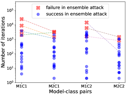
Figure A3: Success or failure of our ensemble attack versus successful per-image PGD attack.

Appendix E Additional Details on Poisoning Attack

Experiment setup.

In our experiment, we generate a synthetic dataset that contains $n=1000$ samples $(\mathbf{z}_{i},t_{i})$. We randomly draw the feature vector $\mathbf{z}_{i}\in\mathbb{R}^{100}$ from $\mathcal{N}(\mathbf{0},\mathbf{I})$, and determine $t_{i}=1$ if ${1}/{(1+e^{-(\mathbf{z}_{i}^{T}\boldsymbol{\theta}^{*}+\nu_{i})})}>0.5$. Here we choose $\boldsymbol{\theta}^{*}=\mathbf{1}$ as the ground-truth model parameters, and $\nu_{i}\in\mathcal{N}(0,10^{-3})$ as random noise. We randomly split the generated dataset into the training dataset $\mathcal{D}_{\mathrm{tr}}$ $(70\%)$ and the testing dataset $\mathcal{D}_{\mathrm{te}}$ $(30\%)$. We specify our learning model as the logistic regression model for binary classification. Thus, the loss function in problem (17) is chosen as $F_{\mathrm{tr}}(\mathbf{x},\boldsymbol{\theta};\mathcal{D}_{\mathrm{tr}})\mathrel{\mathop{:}}=h(\mathbf{x},\boldsymbol{\theta};\mathcal{D}_{\mathrm{tr},1})+h(\mathbf{0},\boldsymbol{\theta};D_{\mathrm{tr},2})$, where $\mathcal{D}_{\mathrm{tr}}=\mathcal{D}_{\mathrm{tr},1}\cup\mathcal{D}_{\mathrm{tr},2}$, $\mathcal{D}_{\mathrm{tr},1}$ represents the subset of the training dataset that will be poisoned, $|\mathcal{D}_{\mathrm{tr},1}|/|\mathcal{D}_{\mathrm{tr}}|$ denotes the poisoning ratio, $h(\mathbf{x},\boldsymbol{\theta};\mathcal{D})=-({1}/{|\mathcal{D}|})\sum_{(\mathbf{z}_{i},t_{i})\in\mathcal{D}}[t_{i}\log(h(\mathbf{x},\boldsymbol{\theta};\mathbf{z}_{i}))+(1-t_{i})\log(1-h(\mathbf{x},\boldsymbol{\theta};\mathbf{z}_{i}))]$, and $h(\mathbf{x},\boldsymbol{\theta};\mathbf{z}_{i})=1/(1+e^{-(\mathbf{z}_{i}+\mathbf{x})^{T}\boldsymbol{\theta}})$. In problem (17), we also set $\epsilon=2$ and $\lambda=10^{-3}$.

In Algorithm A1, unless specified otherwise we choose the the mini-batch size $b=100$, the number of random direction vectors $q=5$, the learning rate $\alpha=0.02$ and $\beta=0.05$, and the total number of iterations $T=50000$. We report the empirical results over $10$ independent trials with random initialization.

Addition results.

In Figure A4, we show the testing accuracy of the poisoned model as the regularization parameter $\lambda$ varies. We observe that the poisoned model accuracy could be improved as $\lambda$ increases, e.g., $\lambda=1$. However, this leads to a decrease in clean model accuracy (below $90\%$ at $\lambda=1$). This implies a robustness-accuracy tradeoff. If $\lambda$ continues to increase, both the clean and poisoned accuracy will decrease dramatically as the training loss in (17) is less optimized.

In Figure A5, we present the testing accuracy of the learnt model under different data poisoning ratios. As we can see, only $5\%$ poisoned training data can significantly break the testing accuracy of a well-trained model.

Figure A4: Empirical performance of ZO-Min-Max in design of poisoning attack: Testing accuracy versus regularization parameter $\lambda$.

Figure A5: Testing accuracy of data poisoning attacks generated by ZO-Min-Max (vs. FO-Min-Max) for different data poisoning ratios.

References

• Aggarwal et al. (2019) Aggarwal, C., Bouneffouf, D., Samulowitz, H., Buesser, B., Hoang, T., Khurana, U., Liu, S., Pedapati, T., Ram, P., Rawat, A., et al. How can ai automate end-to-end data science? arXiv preprint arXiv:1910.14436, 2019.
• Al-Dujaili et al. (2018a) Al-Dujaili, A., Hemberg, E., and O’Reilly, U.-M. Approximating nash equilibria for black-box games: A bayesian optimization approach. arXiv preprint arXiv:1804.10586, 2018a.
• Al-Dujaili et al. (2018b) Al-Dujaili, A., Huang, A., Hemberg, E., and O’Reilly, U.-M. Adversarial deep learning for robust detection of binary encoded malware. In 2018 IEEE Security and Privacy Workshops (SPW), pp. 76–82. IEEE, 2018b.
• Al-Dujaili et al. (2018c) Al-Dujaili, A., Srikant, S., Hemberg, E., and O’Reilly, U.-M. On the application of danskin’s theorem to derivative-free minimax optimization. arXiv preprint arXiv:1805.06322, 2018c.
• Audet & Hare (2017) Audet, C. and Hare, W. Derivative-free and blackbox optimization. Springer, 2017.
• Balasubramanian & Ghadimi (2018) Balasubramanian, K. and Ghadimi, S. Zeroth-order (non)-convex stochastic optimization via conditional gradient and gradient updates. In Advances in Neural Information Processing Systems, pp. 3455–3464, 2018.
• Berahas et al. (2019) Berahas, A. S., Cao, L., Choromanski, K., and Scheinberg, K. A theoretical and empirical comparison of gradient approximations in derivative-free optimization. arXiv preprint arXiv:1905.01332, 2019.
• Bogunovic et al. (2018) Bogunovic, I., Scarlett, J., Jegelka, S., and Cevher, V. Adversarially robust optimization with gaussian processes. In Proc. of Advances in Neural Information Processing Systems, pp.  5765–5775, 2018.
• Boyd & Vandenberghe (2004) Boyd, S. and Vandenberghe, L. Convex optimization. Cambridge university press, 2004.
• Branke & Rosenbusch (2008) Branke, J. and Rosenbusch, J. New approaches to coevolutionary worst-case optimization. In International Conference on Parallel Problem Solving from Nature, pp.  144–153. Springer, 2008.
• Carlini & Wagner (2017) Carlini, N. and Wagner, D. Towards evaluating the robustness of neural networks. In Security and Privacy (SP), 2017 IEEE Symposium on, pp. 39–57. IEEE, 2017.
• Chen et al. (2018) Chen, J., Yi, J., and Gu, Q. A frank-wolfe framework for efficient and effective adversarial attacks. arXiv preprint arXiv:1811.10828, 2018.
• Chen et al. (2017) Chen, P.-Y., Zhang, H., Sharma, Y., Yi, J., and Hsieh, C.-J. Zoo: Zeroth order optimization based black-box attacks to deep neural networks without training substitute models. In Proceedings of the 10th ACM Workshop on Artificial Intelligence and Security, pp.  15–26. ACM, 2017.
• Chen & Giannakis (2018) Chen, T. and Giannakis, G. B. Bandit convex optimization for scalable and dynamic IoT management. IEEE Internet of Things Journal, 2018.
• Chen et al. (2019) Chen, X., Liu, S., Sun, R., and Hong, M. On the convergence of a class of adam-type algorithms for non-convex optimization. International Conference on Learning Representations, 2019.
• Danskin (1966) Danskin, J. M. The theory of max-min, with applications. SIAM Journal on Applied Mathematics, 14(4):641–664, 1966.
• Deng et al. (2009) Deng, J., Dong, W., Socher, R., Li, L.-J., Li, K., and Fei-Fei, L. Imagenet: A large-scale hierarchical image database. In Computer Vision and Pattern Recognition, 2009. CVPR 2009. IEEE Conference on, pp.  248–255. IEEE, 2009.
• Dhurandhar et al. (2019) Dhurandhar, A., Pedapati, T., Balakrishnan, A., Chen, P.-Y., Shanmugam, K., and Puri, R. Model agnostic contrastive explanations for structured data. arXiv preprint arXiv:1906.00117, 2019.
• Duchi et al. (2015) Duchi, J. C., Jordan, M. I., Wainwright, M. J., and Wibisono, A. Optimal rates for zero-order convex optimization: The power of two function evaluations. IEEE Transactions on Information Theory, 61(5):2788–2806, 2015.
• Finlay & Oberman (2019) Finlay, C. and Oberman, A. M. Scaleable input gradient regularization for adversarial robustness. arXiv preprint arXiv:1905.11468, 2019.
• Flokas et al. (2019) Flokas, L., Vlatakis-Gkaragkounis, E.-V., and Piliouras, G. Efficiently avoiding saddle points with zero order methods: No gradients required. arXiv preprint arXiv:1910.13021, 2019.
• Gao et al. (2014) Gao, X., Jiang, B., and Zhang, S. On the information-adaptive variants of the ADMM: an iteration complexity perspective. Optimization Online, 12, 2014.
• Ghadimi & Lan (2013) Ghadimi, S. and Lan, G. Stochastic first-and zeroth-order methods for nonconvex stochastic programming. SIAM Journal on Optimization, 23(4):2341–2368, 2013.
• Ghadimi et al. (2016) Ghadimi, S., Lan, G., and Zhang, H. Mini-batch stochastic approximation methods for nonconvex stochastic composite optimization. Mathematical Programming, 155(1-2):267–305, 2016.
• Gidel et al. (2017) Gidel, G., Jebara, T., and Lacoste-Julien, S. Frank-Wolfe Algorithms for Saddle Point Problems. In Proceedings of the 20th International Conference on Artificial Intelligence and Statistics, volume 54, pp.  362–371. PMLR, 20–22 Apr 2017.
• Golovin et al. (2019) Golovin, D., Karro, J., Kochanski, G., Lee, C., Song, X., et al. Gradientless descent: High-dimensional zeroth-order optimization. arXiv preprint arXiv:1911.06317, 2019.
• Goodfellow et al. (2014) Goodfellow, I. J., Shlens, J., and Szegedy, C. Explaining and harnessing adversarial examples. arXiv preprint arXiv:1412.6572, 2014.
• Hamedani et al. (2018) Hamedani, E. Y., Jalilzadeh, A., Aybat, N. S., and Shanbhag, U. V. Iteration complexity of randomized primal-dual methods for convex-concave saddle point problems. arXiv preprint arXiv:1806.04118, 2018.
• He et al. (2016) He, K., Zhang, X., Ren, S., and Sun, J. Deep residual learning for image recognition. In Proceedings of the IEEE conference on computer vision and pattern recognition, pp.  770–778, 2016.
• Herrmann (1999) Herrmann, J. W. A genetic algorithm for minimax optimization problems. In CEC, volume 2, pp.  1099–1103. IEEE, 1999.
• Ilyas et al. (2018) Ilyas, A., Engstrom, L., Athalye, A., and Lin, J. Black-box adversarial attacks with limited queries and information. arXiv preprint arXiv:1804.08598, 2018.
• Ilyas et al. (2019) Ilyas, A., Engstrom, L., and Madry, A. Prior convictions: Black-box adversarial attacks with bandits and priors. In International Conference on Learning Representations, 2019. URL https://openreview.net/forum?id=BkMiWhR5K7.
• Jagielski et al. (2018) Jagielski, M., Oprea, A., Biggio, B., Liu, C., Nita-Rotaru, C., and Li, B. Manipulating machine learning: Poisoning attacks and countermeasures for regression learning. In 2018 IEEE Symposium on Security and Privacy (SP), pp. 19–35. IEEE, 2018.
• Jensen (2003) Jensen, M. T. A new look at solving minimax problems with coevolutionary genetic algorithms. In Metaheuristics: computer decision-making, pp.  369–384. Springer, 2003.
• Jin et al. (2019) Jin, C., Netrapalli, P., and Jordan, M. I. Minmax optimization: Stable limit points of gradient descent ascent are locally optimal. arXiv preprint arXiv:1902.00618, 2019.
• Jones et al. (2001) Jones, E., Oliphant, T., Peterson, P., et al. SciPy: Open source scientific tools for Python, 2001. URL http://www.scipy.org/.
• Larson et al. (2019) Larson, J., Menickelly, M., and Wild, S. M. Derivative-free optimization methods. Acta Numerica, 28:287–404, 2019.
• Li et al. (2019) Li, Y., Li, L., Wang, L., Zhang, T., and Gong, B. Nattack: Learning the distributions of adversarial examples for an improved black-box attack on deep neural networks. arXiv preprint arXiv:1905.00441, 2019.
• Liu et al. (2018a) Liu, J., Zhang, W., and Yu, N. Caad 2018: Iterative ensemble adversarial attack. arXiv preprint arXiv:1811.03456, 2018a.
• Liu et al. (2018b) Liu, S., Chen, J., Chen, P.-Y., and Hero, A. O. Zeroth-order online admm: Convergence analysis and applications. In Proceedings of the Twenty-First International Conference on Artificial Intelligence and Statistics, volume 84, pp.  288–297, April 2018b.
• Liu et al. (2018c) Liu, S., Kailkhura, B., Chen, P.-Y., Ting, P., Chang, S., and Amini, L. Zeroth-order stochastic variance reduction for nonconvex optimization. In Proc. of Advances in Neural Information Processing Systems, 2018c.
• Liu et al. (2019) Liu, S., Chen, P.-Y., Chen, X., and Hong, M. signSGD via zeroth-order oracle. In Proc. of International Conference on Learning Representations, 2019. URL https://openreview.net/forum?id=BJe-DsC5Fm.
• Liu et al. (2016) Liu, Y., Chen, X., Liu, C., and Song, D. Delving into transferable adversarial examples and black-box attacks. arXiv preprint arXiv:1611.02770, 2016.
• Lu et al. (2019) Lu, S., Tsaknakis, I., and Hong, M. Block alternating optimization for non-convex min-max problems: Algorithms and applications in signal processing and communications. In Proc. of IEEE International Conference on Acoustics, Speech and Signal Processing, pp.  4754–4758, May 2019.
• Lu et al. (2019) Lu, S., Tsaknakis, I., Hong, M., and Chen, Y. Hybrid block successive approximation for one-sided non-convex min-max problems: Algorithms and applications. arXiv preprint arXiv:1902.08294, 2019.
• Madry et al. (2018) Madry, A., Makelov, A., Schmidt, L., Tsipras, D., and Vladu, A. Towards deep learning models resistant to adversarial attacks. ICLR, 2018.
• Moosavi-Dezfooli et al. (2019) Moosavi-Dezfooli, S.-M., Fawzi, A., Uesato, J., and Frossard, P. Robustness via curvature regularization, and vice versa. In Proceedings of the IEEE Conference on Computer Vision and Pattern Recognition, pp.  9078–9086, 2019.
• Nesterov (2007) Nesterov, Y. Dual extrapolation and its applications to solving variational inequalities and related problems. Mathematical Programming, 109(2-3):319–344, 2007.
• Nesterov & Spokoiny (2015) Nesterov, Y. and Spokoiny, V. Random gradient-free minimization of convex functions. Foundations of Computational Mathematics, 2(17):527–566, 2015.
• Nouiehed et al. (2019) Nouiehed, M., Sanjabi, M., Lee, J. D., and Razaviyayn, M. Solving a class of non-convex min-max games using iterative first order methods. arXiv preprint arXiv:1902.08297, 2019.
• Parikh et al. (2014) Parikh, N., Boyd, S., et al. Proximal algorithms. Foundations and Trends® in Optimization, 1(3):127–239, 2014.
• Picheny et al. (2019) Picheny, V., Binois, M., and Habbal, A. A bayesian optimization approach to find nash equilibria. Journal of Global Optimization, 73(1):171–192, 2019.
• Qian et al. (2019) Qian, Q., Zhu, S., Tang, J., Jin, R., Sun, B., and Li, H. Robust optimization over multiple domains. In Proceedings of the AAAI Conference on Artificial Intelligence, volume 33, pp.  4739–4746, 2019.
• Rafique et al. (2018) Rafique, H., Liu, M., Lin, Q., and Yang, T. Non-convex min-max optimization: Provable algorithms and applications in machine learning. arXiv preprint arXiv:1810.02060, 2018.
• Rios & Sahinidis (2013) Rios, L. M. and Sahinidis, N. V. Derivative-free optimization: a review of algorithms and comparison of software implementations. Journal of Global Optimization, 56(3):1247–1293, 2013.
• Sanjabi et al. (2018a) Sanjabi, M., Ba, J., Razaviyayn, M., and Lee, J. D. On the convergence and robustness of training gans with regularized optimal transport. In Proceedings of the 32Nd International Conference on Neural Information Processing Systems, pp.  7091–7101, 2018a.
• Sanjabi et al. (2018b) Sanjabi, M., Ba, J., Razaviyayn, M., and Lee, J. D. On the convergence and robustness of training gans with regularized optimal transport. In Advances in Neural Information Processing Systems, pp. 7091–7101, 2018b.
• Schmiedlechner et al. (2018) Schmiedlechner, T., Al-Dujaili, A., Hemberg, E., and O’Reilly, U.-M. Towards distributed coevolutionary gans. arXiv preprint arXiv:1807.08194, 2018.
• Shamir (2017) Shamir, O. An optimal algorithm for bandit and zero-order convex optimization with two-point feedback. Journal of Machine Learning Research, 18(52):1–11, 2017.
• Steinhardt et al. (2017) Steinhardt, J., Koh, P. W. W., and Liang, P. S. Certified defenses for data poisoning attacks. In Advances in neural information processing systems, pp. 3517–3529, 2017.
• Szegedy et al. (2016) Szegedy, C., Vanhoucke, V., Ioffe, S., Shlens, J., and Wojna, Z. Rethinking the inception architecture for computer vision. In IEEE Conference on Computer Vision and Pattern Recognition (CVPR), pp.  2818–2826, 2016.
• Tran et al. (2018) Tran, B., Li, J., and Madry, A. Spectral signatures in backdoor attacks. In Advances in Neural Information Processing Systems, pp. 8000–8010, 2018.
• Tu et al. (2018) Tu, C.-C., Ting, P., Chen, P.-Y., Liu, S., Zhang, H., Yi, J., Hsieh, C.-J., and Cheng, S.-M. Autozoom: Autoencoder-based zeroth order optimization method for attacking black-box neural networks. arXiv preprint arXiv:1805.11770, 2018.
• Wald (1945) Wald, A. Statistical decision functions which minimize the maximum risk. Annals of Mathematics, pp.  265–280, 1945.
• Wang et al. (2019a) Wang, B., Yao, Y., Shan, S., Li, H., Viswanath, B., Zheng, H., and Zhao, B. Y. Neural cleanse: Identifying and mitigating backdoor attacks in neural networks. Neural Cleanse: Identifying and Mitigating Backdoor Attacks in Neural Networks, pp.  0, 2019a.
• Wang & Wu (2019) Wang, C. and Wu, Q. Flo: Fast and lightweight hyperparameter optimization for automl. arXiv preprint arXiv:1911.04706, 2019.
• Wang et al. (2019b) Wang, J., Zhang, T., Liu, S., Chen, P.-Y., Xu, J., Fardad, M., and Li, B. Towards a unified min-max framework for adversarial exploration and robustness, 2019b.
• Ward et al. (2019) Ward, R., Wu, X., and Bottou, L. AdaGrad stepsizes: Sharp convergence over nonconvex landscapes. In Proceedings of the 36th International Conference on Machine Learning, pp.  6677–6686, 2019.
• Watson & Pollack (2001) Watson, R. A. and Pollack, J. B. Coevolutionary dynamics in a minimal substrate. In Proceedings of the 3rd Annual Conference on Genetic and Evolutionary Computation, pp.  702–709. Morgan Kaufmann Publishers Inc., 2001.