Transition form factors and helicity amplitudes for electroexcitation of negative- and positive parity nucleon resonances in a light-front quark model

Abstract

A workable basis of quark configurations $s^{3}$, $s^{2}p$ and $sp^{2}$ at light front has been constructed to describe the high-$Q^{2}$ behavior of transition form factors and helicity amplitudes in the electroproduction of the lightest nucleon resonances, $N_{1/2^{-}}(1535)$ and $N_{1/2^{+}}(1440)$. High-quality data of the CLAS Collaboration are described in the framework of a model which takes into account mixing of the quark configurations and the hadron-molecular states. The model allows for a rough estimate of the quark core weight in the wave function of the resonance in a comparison with high momentum transfer data on resonance electroproduction.

I Introduction

New data on the electroproduction of low-lying nucleon resonances ($J^{P}=\frac{1}{2}^{\pm}$,$\frac{3}{2}^{\pm}$,$\frac{5}{2}^{\pm}$) at large momentum transfer provide important complementary information on the inner structure of hadron resonances Aznauryan:2008pe -Burkert:2018oyl . These data provide evidence in support of the dominance of quark degrees of freedom in the process of electroproduction and allow to evaluate the weight of the quark component in the resonance wave function. The resonance spectrum is remarkably consistent with the quark-model predictions Isgur:1978wd , but the traditional quark model refers only to the rest frame, whereas processes at large momentum transfer require a description of baryons in the moving frame. There are many theoretical approaches  to the problem which start from the first principles Brodsky1998 -Gutsche:2019lyu , e.g., light-front QCD Brodsky1998 , lattice QCD Lin:2008qv , quark models Aznauryan:2012ec -Ramalho:2018wal , light-cone sum rules Braun:2009jy , approaches based on solution of Dyson-Schwinger and Bethe-Salpeter equations Roberts:2018hpf ; Burkert:2019bhp , approaches based on chiral dynamics Jido:2007sm , AdS/QCD deTeramond:2011qp -Gutsche:2019lyu .

The LF wave functions have the advantage that they undergo interaction-independent transformations under the action of ”front boosts”. In the front form of dynamics Dirac1949 the generators of front boosts are kinematical and the front boosts itself are elements of a kinematical subgroup of the Poincaré group. The price to pay is that the space rotations are not kinematical transformations. The light front $t-z=\,$0 is not invariant under space rotations except for rotations about the $z$ axis. Thus the generators of rotations should depend on the interaction given at the light front. By contrast, in the instant form of dynamics the ”instant” ($t=0$), or canonical, boosts depend on the interaction and do not generate a kinematical subgroup. Then the rotation group (together with the spatial translation group) can be considered as a kinematical subgroup of the Poincaré group.

In spite of difficulties associated with the rotational symmetry, the LF approach to the description of the transition form factors implies the construction of a good basis of quark configurations possessing definite values of the orbital ($L$) and total ($J=L+S$) angular momenta and satisfying the Pauli exclusion principle. The challenge has been to modify the standard shell-model (normally harmonic oscillator) basis to describe the LF three-quark configurations with simple properties about the relativistic boosts and without the rotational symmetry in an ordinary sense. Many works Aznauryan1982 ; Weber1990 ; Chung:1991st ; JuliaDiaz:2003gq ; Cardarelli:1996gi ; Schlumpf:1992ce ; Brodsky:1994aw ; Capstick:1994ne ; Aznauryan:2012ba ; Aznauryan:2012ec ; Obukhovsky:2013fpa have succeeded in solving this problem. Now there exist a lot of works  JuliaDiaz:2003gq ; Capstick:1994ne ; Aznauryan:2012ba ; Aznauryan:2012ec ; Obukhovsky:2013fpa ; Ramalho:2018wal where the recent high-quality data of the CLAS Collaboration  Aznauryan:2008pe ; Aznauryan:2009mx ; Mokeev:2015lda ; Park:2014yea ; Dalton2009 ; Armstrong2009 ; Denizl2007 ; Burkert2003 ; Thompson2001 ; Dugger2009 on the $N+\gamma^{*}\to N^{*}$ transition amplitudes have been successfully described at high momentum transfer in terms of the covariant formalism.

A key role in the construction of the basis of quark configurations at light front plays a specific formalism which might be considered as an analogue of the nonrelativistic technique of Clebsch-Gordan coefficients and spherical functions. Such a formalism was developed in the last century in terms of irreducible representations of the Poincaré group. In the rest frame, the sum of the spin and the orbital angular momenta of a two-particle system can be readily defined in terms of the standard Clebsch-Gordon coefficients and the spherical functions Shirokov1959 . A useful generalization of such a definition of the sum for a three(few)-body system at light front has been taken to develop a more complicated technique. Such a development began with works of Teremt’ev, Berestetsky, Kondratyuk and Bakker Berestetskii1976 ; Bakker1979 ; Kondratyuk1980 in the 70-s and ended with the Hamiltonian dynamics at light front of Keister and Polyzou Keister1991 (and also with works of many authors later on). Note the review Polyzou2013 , where the problem of constructing Clebsch-Gordan coefficients for the Poincaré group was discussed in the framework of the formalism developed in Keister1991 and where a general expression for adding single-particle spins and orbital angular momenta has been given.

The formalism involves all elements that are necessary to construct a workable basis of quark configurations except for the requirement imposed by the Pauli exclusion principle. The realization of this requirement is trivial in the case of zero orbital momentum, but in the case of $L\geq\,$1 particular attention should be given to configurations with the proper types of permutational symmetry (e.g. the Young schemes and the Yamanouchi symbols). The LF approach to the description of reactions $N+\gamma^{*}\to N^{*}$ at large momentum transfer was successfully realized in many works Weber1990 ; Chung:1991st ; JuliaDiaz:2003gq ; Cardarelli:1996gi ; Schlumpf:1992ce ; Brodsky:1994aw ; Capstick:1994ne ; Aznauryan:2012ba ; Aznauryan:2012ec ; Obukhovsky:2013fpa . But in all works, where the above formalism was used in the case of $L\geq\,$1, the orbitally excited quark configurations have not been discussed in detail. Without a detailed representation of the wave function it is not evident that, coinciding with the given values of $L$ and $J$, the quark configuration satisfies the Pauli exclusion principle.

Here we compensate this gap and construct a workable basis of the LF quark configurations $s^{3}$, $s^{2}p$ and $sp^{2}$ that satisfies the Pauli exclusion principle. We use this basis to represent the LF wave functions of the nucleon and the low-lying resonances of opposite parity, $N_{1/2^{-}}^{*}$ and $N_{1/2^{+}}^{*}$. Finally we went to describe elastic and transition form factors on a common footing. The phenomenological wave functions used in the expansion of baryon states in terms of this basis have a common radial part $\Phi_{0}$ times an angular (or polynomial) factor — in full analogy with the non-relativistic shell-model wave functions. The function $\Phi_{0}$ (the baryon ”quark core”) differs from the Gaussian usually used in quark models. We use a pole-like wave function Schlumpf:1992ce , the free parameters of which are fitted by data on the elastic nucleon form factors in a large interval of 0$\leq Q^{2}\lesssim\,$32 GeV² Schlumpf:1992ce ; Obukhovsky:2013fpa .

At moderate momentum transfers, i.e. for $Q^{2}\lesssim\,$1 - 2 GeV², a good description of elastic and transition form factors can be obtained in an equivalent manner by using different representations of $\Phi_{0}$, with Gaussian Aznauryan:2012ec ; Obukhovsky:2011sc , pole-like Schlumpf:1992ce or hyper central Santopinto:2012nq wave functions, and also by addition of other degrees of freedom Aznauryan:2012ec ; Obukhovsky:2011sc ; Aiello1998 or by expanding the quark basis Capstick:1994ne . At the high momentum transfers the details of the inner structure are not so important and the $Q^{2}$ behavior of form factors is only determined by the high-momentum components of the wave function. Note that in the region of asymptotically high momenta a key role in the $Q^{2}$ behavior of form factors plays the contribution of leading gluon-exchange diagrams Brodsky:1976rz and, conceivably, the dependence of the running (dynamical) quark mass on the quark momentum Burkert:2018oyl ; Burkert:2019bhp ; Aznauryan:2012ec . We assume that the phenomenological wave function $\Phi_{0}$, the free parameters of which are fitted to the high-momentum behavior of the nucleon form factors, could effectively take into account such ”QCD contributions”. These contributions should be, in general, the same both for the nucleon and the low-lying nucleon resonances. Thus we use a common wave function $\Phi_{0}$ as a first approximation in both cases and compare the calculated transition amplitudes to the high-quality CLAS data Aznauryan:2008pe ; Aznauryan:2009mx ; Mokeev:2015lda ; Park:2014yea ; Dalton2009 ; Armstrong2009 ; Denizl2007 ; Burkert2003 ; Thompson2001 ; Dugger2009 in the region $Q^{2}\gtrsim\,$1 - 2 GeV².

A comparison shows that even in a first step, where one uses a model without new free parameters beyond those that were fitted to the elastic form factors, one obtains a realistic description of all the transition form factors at high momentum transfers up to the maximal values of $Q^{2}\simeq 5-7$ GeV² achieved in the CLAS experiment. Therefore, the quark shell model at light front with a specific (pole-like) wave function for the nucleon quark core is a realistic model for the description of electromagnetic processes on the nucleon at high momentum transfers. The model could be used for the prediction of the transition form factors at higher $Q^{2}$ and for the evaluation of momentum distributions of valence quarks in the state with nonvanishing values of orbital angular momentum.

Starting from this realistic model we evaluate permissible values of the mixing parameters for the hadron-molecular components $N+\sigma$ and $\Lambda+K$ in the nucleon resonances $N_{1/2^{+}}^{*}$ and $N_{1/2^{-}}^{*}$ respectively. We show that only two complimentary free parameters are needed to improve the description of the $Q^{2}$ behavior of helicity amplitudes for the Roper resonance and to obtain a good agreement with all experimental data at $Q^{2}\gtrsim\,$1-2 GeV². The modified wave function of the Roper resonance has a spatially wider distribution than the wave function of the nucleon.

The paper is organized as follows. In Sect. II and Appendix A we briefly discuss the formalism developed in Refs. Keister1991 ; Polyzou2013 . Following these references we represent the basic formulas and definitions for the sector of one- and two-particle LF states. In Sec. III we consider three-quark LF configurations for the cases, in which the total orbital angular momentum L does not exceed the value $l=\,$1. We construct the three-quark basis states following step by step the method developed in Sect. II for the two-quark systems. In Sect. IV the spin-orbital basis states constructed in Sect. III are supplemented by the isospin part and a workable method for constructing the basis satisfying the Pauli exclusion principle is developed. Matrix elements of the one-particle quark current between basis states of LF quark configurations are represented by sums of six-dimensional integrals of four different types. These result in expressions for the Dirac ($F_{1}$) and Pauli ($F_{2}$) form factors of the transitions with/without change of baryon parity. In Sect. V the values of helicity amplitudes and Dirac/Pauli transition form factors for the electroexcitation of resonances $N_{1/2^{-}}(1535)$ and $N_{1/2^{+}}(1440)$ are expressed in terms of quark transition amplitudes defined in Sect. IV. In Sect. VI the results of the calculations are compared with CLAS data and concluding remarks are given.

II Formalism

We have taken the formalism developed in Refs. Keister1991 ; Polyzou2013 as a starting point for our study of light front quark configuration. In this section we represent only basic formulas and definitions of the formalism Keister1991 ; Polyzou2013 that will be very useful for the short presentation of our results in the following sections. We use notations which are very close to those used in Refs. Keister1991 ; Polyzou2013 .

II.1 Definitions and notations

Quark state vectors $|(m_{i},s_{i});\bm{p}_{i},\mu_{i}\rangle$ are defined as the basis states of an unitary irreducible representation of the Poincaré group characterized by two invariants, $m_{i}^{2}$ and $s_{i}(s_{i}+1)$, which are the proper values of operators $M^{2}=P^{\mu}P_{\mu}$ (square of the mass) and $-\frac{1}{M^{2}}W^{\mu}W_{\mu}$ (square of spin). The 4-vector $W^{\mu}$ is the Pauli-Lyubansky vector

$$W^{\mu}=-\frac{1}{2}\varepsilon^{\mu\alpha\beta\gamma}P_{\alpha}J_{\beta\gamma}$$ (1)

and $P^{\mu}$ and $J^{\mu\nu}$ are generators of the Poincaré group. In the case of a three-quark system one can use the equations $\bm{P}=\bm{p}_{1}+\bm{p}_{2}+\bm{p}_{3}$, $P^{0}=\sqrt{\bm{P}^{2}+M^{2}}$, where $p_{i}^{\mu}$ is a quark momentum on its mass shell $p_{i}^{0}=\omega_{i}(\bm{p}_{i}):=\sqrt{\bm{p}_{i}^{2}+m_{i}^{2}}$. Starting from the direct products of these ”plane-wave” quark states $\stackrel{{\scriptstyle 3}}{{\prod}}_{i\!=\!1}\!\!|(m_{i},s_{i});\bm{p}_{i},\mu_{i}\rangle$, we can construct the two- and three-quark basis vectors

$$|[m_{12},j_{12}(l_{12},s_{12})];\bm{P}_{12},\mu_{12}\rangle,\quad|[M_{0},j((j_{12}(l_{12},s_{12}),s_{3}),l_{3})];\bm{P},\mu_{j}\rangle.$$ (2)

These states have definite values for the orbital angular momentum ($l_{12}$), the spin ($s_{12}$) and the sum of them $j_{12}=l_{12}+s_{12}$ for two-quark clusters ($\bm{P}_{12}=\bm{p}_{1}+\bm{p}_{2}$) and a definite value for the total angular momentum $j=j_{12}+s_{3}+l_{3}$ of the three-quark system. Here $m_{12}$ and $M_{0}$ are masses of two- and three-quark free states, respectively.

Two-particle basis vectors of the irreducible representation $j_{12}(l_{12},s_{12})$ of the rotation group can be constructed Shirokov1959 in the rest frame, where $\bm{P}_{12}=\bm{\stackrel{{\scriptstyle\circ}}{{P}}}_{12}:=\bm{0}$, using standard methods of nonrelativistic quantum mechanics (the Clebsch-Gordan coefficients and spherical functions $Y_{l\mu_{l}}(\bm{\hat{p}}_{1})$). Setting up the basis of the three-particle irreducible representation $j((j_{12}(l_{12},s_{12}),s_{3}),l_{3})$ with the same method requires to pass into the three-particle rest frame, where $\bm{P}=\bm{\stackrel{{\scriptstyle\circ}}{{P}}}:=\bm{0}$, but $\bm{P_{12}}\neq\,$0. This requires a relativistic boost on the two-quark cluster to transform its wave function into the moving (with the 4-velocity $P_{12}^{\mu}/m_{12}$) frame.

The construction of the irreducible representations of the Poincaré group is performed in the centre of mass (CM) frame where $P^{\mu}=\{M,\bm{0}\}$. A special role of the rest frame in construction of the basis of irreducible representations of the Poincaré group stems from the fact that only in this frame the 4-vector of spin given in Eq. (1) reduces to 3-vector $\frac{1}{M}W^{\mu}=\{0,J^{23},J^{31},J^{12}\}$ which coincides with the 3-vector of rotation generators $J^{ij}$. Thus one can use a standard technique of the rotation group to construct the basis vectors. The inner relative momenta of a baryon can be specified by the quark momenta $\bm{k}_{i}$, $i=\,$1,2.3 in the baryon CM frame, $\bm{k}_{1}+\bm{k}_{2}+\bm{k}_{3}=\bm{\stackrel{{\scriptstyle\circ}}{{P}}}:=\bm{0}$ (we use letters $k$ or $K$ for the relative momenta as done in the literature Keister1991 ; Polyzou2013 ; Capstick:1994ne ). The inner relative momenta of the two-quark cluster are specified by the quark momenta ${\bm{k}}_{1}^{\prime}$ and ${\bm{k}}_{2}^{\prime}$ in its rest frame ($\stackrel{{\scriptstyle\circ}}{{P}}_{12}^{\mu}=\{m_{12},\bm{0}\}$),

$$\bm{k_{1}^{\prime}}=\Lambda^{-1}(\frac{\bm{k_{1}}+\bm{k_{2}}}{m_{12}})\bm{k_{1}}=\bm{k}\quad\mbox{É}\quad\bm{k_{2}^{\prime}}=\Lambda^{-1}(\frac{\bm{k_{1}}+\bm{k_{2}}}{m_{12}})\bm{k_{2}}=-\bm{k},$$ (3)

where $\Lambda(\frac{\bm{p}}{m})\equiv\Lambda^{\mu}_{\nu}$ is the matrix of the Lorentz transformation that describes the transition from the two-quark rest frame to the moving frame (the value $\frac{P_{12}^{\mu}}{m_{12}}\equiv\frac{(k_{1}+k_{2})^{\mu}}{m_{12}}$ is a 4-velocity of the two-quark cluster in the baryon CM frame). The 3-momentum $\bm{k}$ defined by Eq. (3) is one of two independent relative momenta in the three-quark system. A second independent relative momentum may be identified with the momentum $\bm{K}:=\bm{k_{3}}=\!-(\bm{k_{1}}\!+\!\bm{k_{2}})$. Masses $m_{12}$ and $M_{0}$ of the two- and three-quark clusters in the baryon,

$$m_{12}(\bm{k})=\omega_{1}(\bm{k})+\omega_{2}(-\bm{k})\quad\mbox{É}\quad M_{0}(\bm{k},\bm{K})=\omega_{1}(\bm{k}_{1})+\omega_{2}(\bm{k}_{2})+\omega_{3}(\bm{k}_{3}),$$ (4)

are functions of two independent relative momenta $\bm{k}$ and $\bm{K}$. The state vector of the baryon in its rest frame ($\bm{P}=\bm{\stackrel{{\scriptstyle\circ}}{{P}}}$) may be symbolically (we omit isospin and other details) represented in terms of a superposition of free basis vectors (2)

$$|(M,j);\bm{\stackrel{{\scriptstyle\circ}}{{P}}},\mu_{j}\rangle\sim\int k^{2}dkK^{2}dK\Phi_{M,j}(M_{0})|[M_{0},j((j_{12}(l_{12},s_{12}),s_{3}),l_{3})];\bm{\stackrel{{\scriptstyle\circ}}{{P}}},\mu_{j}\rangle.$$ (5)

$\Phi_{Mj}$ is a wave function that should depend on an invariant combination of two relative momenta, $\bm{k}$ and $\bm{K}$. The free mass $M_{0}$ defined in Eq.(4) may be used as such an invariant combination. For example, the wave function $\Phi_{Mj}(M_{0})$ could be a solution of the three-particle relativistic equation in the framework of the Bakamjian-Thomas Bakamjian1953 approach or it could be a phenomenological wave function.

The important property of the integrand in r.h.s. of Eq. (5) is that the three-quark basis state, denoted by proper values of orbital/total angular momenta, can be represented as a superposition of free three-quark plane-wave states $\stackrel{{\scriptstyle 3}}{{\prod}}_{i\!=\!1}\!\!|(m_{i},s_{i});\bm{p}_{i},\mu_{i}\rangle$ (see later for details) which itself realizes the irreducible representation of the Poincaré group. Therefore the transformation of the state vector (5) into a moving reference frame $\bm{\stackrel{{\scriptstyle\circ}}{{P}}}\to\bm{P}\neq\bm{0}$ can be readily done by the unitary representation $U[\Lambda_{g}(\frac{\bm{P}}{M_{0}})]$ of the one-particle boost $\Lambda_{g}(\frac{\bm{P}}{M_{0}})$ in plane-wave basis $|(m_{i},s_{i});\bm{p}_{i},\mu_{i}\rangle$ Here $\frac{\bm{P}}{M_{0}}$ is the spatial part of the 4-velocity $u^{\mu}=\frac{1}{M_{0}}\{P^{0},\!\bm{P}\}$ and the index $g$ above specifies the little group used for the transition $\bm{\stackrel{{\scriptstyle\circ}}{{P}}}\to\bm{P}$ (see definitions of the canonical and front boosts in Appendix A).

II.2 Two-particle states and Melosh transformations

The basis state vectors of the irreducible representation $j(ls)$ of the rotation group can be constructed in the rest frame of the two-particle cluster with the standard non-relativistic technique of adding angular momenta (Clebsch-Gordan coefficients and spherical functions) Keister1991 ; Polyzou2013 ; Shirokov1959 :

$$|[m_{12}(k),j(l,s)];\bm{\stackrel{{\scriptstyle\circ}}{{P}}}_{12},\mu_{j}\rangle=\sum_{\{\mu\}}(s_{1}\mu_{1}s_{2}\mu_{2}|s\mu_{s})(l\mu_{l}s\mu_{s}|j\mu_{j})\!\int\!\!d^{2}{\hat{k}}Y_{l\mu_{l}}(\hat{k})|\bm{k},\mu_{1}\rangle_{\!c}|\mbox{-}\bm{k},\mu_{2}\rangle_{\!c},$$ (6)

where $\{\mu\}:=\mu_{1},\mu_{2},\mu_{s},\mu_{l}$ and $m_{12}$ is a mass defined in Eqs. (4) and (62). The state vector of the physical two-particle system (e.g., a bound state) can be expanded in the basis (6) and represented in form of

$$|[m_{d},j(l,s)];\bm{\stackrel{{\scriptstyle\circ}}{{P}}}_{12},\mu_{j}\rangle=\int_{0}^{\infty}\frac{k^{2}dk}{(2\pi)^{3}}\Phi_{j(ls)}[m_{12}(k)]|[m_{12}(k),j(l,s)];\bm{\stackrel{{\scriptstyle\circ}}{{P}}}_{12},\mu_{j}\rangle,$$ (7)

where $m_{d}$ is the mass of the bound state and $\Phi_{j(ls)}$ is the wave function.

The canonical basis vectors $|\pm\bm{k},\mu_{i}\rangle_{\!c}$ in the r.h.s. of Eq. (6) can be transformed into the moving reference frame $\bm{\stackrel{{\scriptstyle\circ}}{{P}}}_{12}\to\bm{P}_{12}$ by making use of the transformation formula of Eq. (55). But such a transformation is complicated by the Wigner rotation which depends on both the initial and finite momenta of the $i$-th quark. Thus, it would be the more convenient to pass to the front form of the state vector (7) immediately after the determination of the basis vectors of the irreducible representation $j(ls)$ in Eq. (6). Then one can use the simpler formula of Eq. (56) for the transition $\bm{\stackrel{{\scriptstyle\circ}}{{P}}}_{12}\to\bm{P}_{12}$. An additional complication is the Melosh transformation Melosh1974

$$|(m_{i},s_{i});\bm{k}_{i},\mu_{i}\rangle_{\!c}=\sqrt{\frac{k_{i}^{+}}{\omega_{i}(k_{i})}}\sum_{\bar{\mu}_{i}}|(m_{i},s_{i});\bm{\tilde{k}}_{i},\bar{\mu}_{i}\rangle_{\!f}D^{(s_{i})}_{\bar{\mu}_{i}\mu_{i}}[R_{fc}(k_{i})],$$ (8)

where $R_{fc}(k_{i})$ is the space rotation which connects the front spin of the quark and its canonical spin. In the case of $s_{i}=\frac{1}{2}$ the respective D matrix is equal to the matrix element

$$D^{(1/2)}_{\bar{\mu}_{i}\mu_{i}}[R_{fc}(k_{i})]=\langle\frac{1}{2},\tilde{\mu}_{i}|\frac{m_{i}+k_{i}^{+}-i\hat{z}[\bm{\sigma}_{i\bot}\!\!\times\!\bm{k}_{i\bot}]}{\sqrt{2k_{i}^{+}(\omega_{i}(k_{i})+m_{i})}}|\frac{1}{2},\mu_{i}\rangle$$ (9)

where $\tilde{\mu}_{i}$ and $\mu_{i}$ are the $z$-components of the front and canonical spins, respectively.

The final expression for the basis vector (6) in the moving reference frame is of the form

$$\!\!\!\!\!\!\!\!\!\!\sqrt{\frac{P^{+}_{12}}{m_{12}}}|[m_{12},j(l,s)];\bm{\tilde{P}}_{12},\mu_{j}\rangle_{\!f}:=U[\Lambda_{f}(\frac{\bm{\tilde{P}}_{12}}{m_{12}})]|\bm{\stackrel{{\scriptstyle\circ}}{{P}}}_{12},\mu_{j}\rangle=\sqrt{\!\frac{p_{1}^{+}p_{2}^{+}}{\omega_{1}(\bm{k})\omega_{2}(\!-\!\bm{k})}}\sum_{\{\mu\}}(s_{1}\mu_{1}s_{2}\mu_{2}|s\mu_{s})$$ (10)

$$\times \!\!\!(l\mu_{l}s\mu_{s}|j\mu_{j})\!\!\int\!\!d^{2}{\hat{k}}Y_{l\mu_{l}}(\hat{k})\sum_{\bar{\mu}_{1}\bar{\mu}_{2}}|\bm{\tilde{p}}_{1},\bar{\mu}_{1}\rangle_{\!f}|\bm{\tilde{p}}_{2},\bar{\mu}_{2}\rangle_{\!f}D^{(1/2)}_{\bar{\mu}_{1}\mu_{1}}[R_{fc}(k_{1})]D^{(1/2)}_{\bar{\mu}_{2}\mu_{2}}[R_{fc}(k_{2})],$$

where $\bm{\tilde{p}}_{1}=\Lambda_{f}(\frac{\tilde{P}_{12}}{m_{12}})\bm{\tilde{k}}$, $\bm{\tilde{p}}_{2}=\Lambda_{f}(\frac{\tilde{P}_{12}}{m_{12}})(\!-\!\bm{\tilde{k}})$. The components of the 3-vector of the relativistic relative momentum $k^{j}=\{\bm{k}_{\bot},k_{z}\}$ are also expressed in terms of invariants, $k_{z}:=\frac{1}{2}(k^{+}-k^{-})=\frac{1}{2}\left[xm_{12}-\frac{\bm{k}_{\bot}^{2}+m^{2}}{xm_{12}}\right]$, $x=\frac{k^{+}}{P_{12}^{+}}$, $\hat{k}\!=\!\frac{\bm{k}}{|\bm{k}|}$.

Since the wave function $\Phi_{j(ls)}$ and its argument $m_{12}$ are relativistic invariants, the expression for the state vector (7) in a moving reference frame, $\sqrt{\frac{P_{12}^{+}}{m_{d}}}|[m_{d},j(l,s)];\bm{\tilde{P}}_{12},\mu_{j}\rangle_{\!f}$, can be obtained by the substitution $|[m_{12},j(l,s)];\bm{\stackrel{{\scriptstyle\circ}}{{P}}}_{12},\mu_{j}\rangle\to\sqrt{\frac{P^{+}_{12}}{m_{12}}}|[m_{12},j(l,s)];\bm{\tilde{P}}_{12},\mu_{j}\rangle_{\!f}$ in the r.h.s. of Eq. (7).

III Three-particle basis states

Here we consider three-quark configurations at the light front for cases when the total orbital angular momentum is not larger than $l=\,$1. Then there are three simple variants: $\{l\!=\!0(l_{12}\!=l_{3}=\!l)\}$, $\{l\!=\!0(l_{12}\!=l_{3}=\!1)\}$ and $\{l\!=\!1[(l_{12}\!=\!0,l_{3}\!=\!l),(l_{12}\!=\!l,l_{3}\!=\!0)]\}$. The more complicated variant $\{l\!=\!1(l_{12}\!=l_{3}=\!l)\}$ is omitted as here we only consider the lowest excited state for each given parity $P=\pm$. This is the minimal basis to evaluate the transition form factors for the low-lying resonances $N_{1/2^{+}}(1440)$ and $N_{1/2^{-}}(1535)$ along with the elastic nucleon form factors. These configurations are the analogues to the non-relativistic translationally-invariant shell-model (TISM) configurations $s^{3}[3]_{X}(l\!\!=\!\!0)$, $sp^{2}[3]_{X}(l\!\!=\!\!0)$ and $s^{2}p[21]_{X}(l\!\!=\!\!1)y_{X}^{(n)}(n=1,2)$, respectively. The Young tableaux $[f]_{X}$ in the coordinate (orbital) space (X) and the Yamanouchi symbols $y_{X}^{(n)}$ are used in the TISM for classification of multi-particle states. Such a classification plays a key role in the construction of basis states satisfying the Pauli exclusion principle. In this case the quark configuration for the baryon of negative parity ($\underline{70}^{-},[21]_{X},l=\,$1) should be constructed in two variants, with the Yamanouchi symbols $y^{(1)}_{X}=\{112\}$ (symmetric under permutation $P_{ij}$ of the two first quarks, ij=12, i.e. $|l_{12}\!=\!0,\,l_{3}\!=\!1\rangle$) and $y^{(2)}_{X}=\{121\}$ (antisymmetric under the permutation $P_{12}$, e.g. $|l_{12}\!=\!1,\,l_{3}\!=\!0\rangle$). Then a fully antisymmetric state in the product of all subspaces $X\circ S\circ T\circ C$ ($S$-spin, $T$-isospin, $C$-color) can be readily constructed with the use of the permutation group $S_{3}$ technique Hamermesh1964 .

We construct the three-quark basis states following step by step the method developed in Sect. II for the two-quark state vectors. In the case of low angular momenta $l=\,$0, 1 the three-quark basis vectors are of the same form as the two-quark states given in Eqs. (6) and (10)). Starting from these expressions one can at once write the three-quark basis state having the quantum numbers of the TISM configuration $s^{2}p[21]_{X}(l\!=\!1)y_{X}^{(1)}$ (i.e. $l_{12}\!=\!0,l_{3}\!=\!1$):

$$\!|[21]_{X}y_{X}^{(1)}[M_{0},j(l,s(s_{12}))];\bm{\tilde{P}},\mu_{j}\rangle_{\!f}=\!\int d^{2}\hat{K}{\tilde{\cal J}}(p^{+}\!,k)\!\left(\frac{K}{\beta\!}\right)^{\!l}\!\sum_{\{\mu\}}Y_{l\mu_{l}}(\hat{K})$$ (11)

$$\!\!\!\!\!\!\!\!\!\!\times \!\!\!\!\!\!\left\{\!(\frac{1}{2}\mu_{1}\frac{1}{2}\mu_{2}|s_{12}\mu_{12})(s_{12}\mu_{12}\frac{1}{2}\mu_{3}|s\mu_{s})(l\mu_{l}s\mu_{s}|j\mu_{j})\sum_{\bar{\mu}}\prod_{i\!=\!1}^{3}|\bm{\tilde{p}}_{i},\bar{\mu}_{i}\rangle_{\!f}D^{(\frac{1}{2})}_{\bar{\mu}_{i}\mu_{i}}[R_{fc}(k_{i})]\!\right\}\!\!,\,l\!=\!1,$$

where $\bm{\tilde{p}}_{i}=\Lambda_{f}(\frac{P}{M_{0}})\bm{\tilde{k}}_{i}$, $\bm{\tilde{P}}=\bm{\tilde{p}}_{1}+\bm{\tilde{p}}_{2}+\bm{\tilde{p}}_{3}$, $\bm{\tilde{K}}=\bm{\tilde{k}}_{3}$, $\bm{K}\!=\!\{\bm{K}_{\bot},K_{z}\}$, $K_{z}\!=\!\frac{1}{2}(K^{+}\!-\!K^{-}\!)=\!\frac{1}{2}\left((1\!-\!\eta)M_{0}\!-\!\frac{K_{\bot}^{2}+m_{3}}{(1\!-\!\eta)M_{0}}\right)$, ${\tilde{\cal J}}(p^{+},k)=\sqrt{\!\frac{p_{1}^{+}p_{2}^{+}p_{3}^{+}M_{0}}{\omega_{1}(\bm{k}_{1})\omega_{2}(\bm{k}_{2})\omega_{3}(\bm{k}_{3})P^{+}}}$. Here $\beta$ is an arbitrary scale (the nucleon inverse radius as usual).

The three-quark LF state vector analogous to the TISM configuration $s^{2}p[21]_{X}(l\!=\!1)y_{X}^{(1)}$ is defined by an expression which is a replica of Eq. (7):

$$\!\!\!\!|s^{2}p[21]_{X}y_{X}^{(1)}[M,j(l,s(s_{12}))];\bm{\tilde{P}},\mu_{j}\rangle_{\!f} = \!\int\frac{d^{3}k}{(2\pi)^{3}}\int_{0}^{\infty}\!\frac{K^{2}dK}{(2\pi)^{3}}{\cal N}_{l}^{(1)}\Phi_{0}(M_{0})$$ (12)

$$\times |s^{2}p[21]_{X}y_{X}^{(1)}[M_{0},j(l,s(s_{12}))];\bm{\tilde{P}},\mu_{j}\rangle_{\!f},\,\,l=1,$$

where the wave function $\Phi_{0}(M_{0})$ describes the radial part of the configuration. Note that like the TISM configurations $s^{3}$, $s^{2}p$, $\dots$ etc. the respective LF configurations have a common radial part which is the same as the radial wave function $\Phi_{0}(M_{0})$ of the ground state configuration $s^{3}$. The normalization factor ${\cal N}_{l}^{(1)}$ in the r.h.s. of Eq. (12) may be calculated using the normalization condition determined in Eq. (52).

In the case of $l\!=\!1(l_{12}\!=\!l,l_{3}\!=\!0)$ the basis vector with the quantum numbers of the TISM state $s^{2}p[21]_{X}(l\!=\!1)y_{X}^{(2)}$ is of the form

$$|[21]_{X}y_{X}^{(2)}[M_{0},j(l,s(s_{12}))];\bm{\tilde{P}},\mu_{j}\rangle_{\!f}=\!\int d^{2}\hat{k}\tilde{\cal J}(p,k)\!\left(\!\!\frac{k}{\beta\!}\!\right)^{\!\!l}\!\sum_{\{\mu\}}Y_{l\mu_{l}}(\hat{k})\{\,\,\dots\,\,\},\,\,l=1,$$ (13)

where $\bm{k}$ is a relative momentum defined in Eqs. (3) and (59) - (61). Dots in the curly brackets denote the same expression as in the curly brackets of Eq. (11). The LF state vector analogous to the TISM configuration $s^{2}p[21]_{X}(l\!=\!1)y_{X}^{(2)}$ is defined by an equation similar to Eq. (12):

$$\!\!\!\!|s^{2}p[21]_{X}y_{X}^{(2)}[M,j(l,s(s_{12}))];\bm{\tilde{P}},\mu_{j}\rangle_{\!f} = \!\int\frac{d^{3}K}{(2\pi)^{3}}\int_{0}^{\infty}\!\frac{k^{2}dk}{(2\pi)^{3}}{\cal N}_{l}^{(2)}\Phi_{0}(M_{0})$$ (14)

$$\times |s^{2}p[21]_{X}y_{X}^{(2)}[M_{0},j(l,s(s_{12}))];\bm{\tilde{P}},\mu_{j}\rangle_{\!f},\,\,l=1.$$

In the case of $l\!=\!0(l_{12}\!=l_{3}=\!l)$ the basis vectors $|s^{3}[3]_{X}[M_{0},j(l\!=\!0,s(s_{12}))];\bm{\tilde{P}},\mu_{j}\rangle_{\!f}$ and the state vector $|[3]_{X}[M,j(l\!=\!0,s(s_{12}))];\bm{\tilde{P}},\mu_{j}\rangle_{\!f}$ are also defined by Eqs. (11) and (12), respectively, but with the other value of $l=0$ and with the spherical wave function $Y_{00}=\sqrt{\frac{1}{4\pi}}$. In this case the radial part of the LF configuration $s^{3}[3]_{X}$ (a nucleon, the ground state) is described by the wave function $\Phi_{0}(M_{0})$. The radial part of the excited LF configuration $sp^{2}[3]_{X}(l\!=\!0)$ (the Roper resonance $N_{1/2^{+}}^{*}$) is described by function $\Phi_{02}(M_{0})={\cal N}_{02}(1\!\!-\!c_{2}\!\frac{M_{0}^{2}}{\beta^{2}})\Phi_{0}(M_{0})$, where a free parameter $c_{2}$ is chosen to satisfy the orthogonality condition $\langle N_{1/2^{+}}^{*}|N\rangle=\,$0.

The main drawback of the configurations $|s^{2}p[21]_{X}y_{X}^{(1)}\rangle$ and $|s^{2}p[21]_{X}y_{X}^{(2)}\rangle$ defined as orbital states $l\!=\!1(l_{12}\!=\!0,l_{3}\!=\!1)$ and $l\!=\!1(l_{12}\!=\!1,l_{3}\!=\!0)$ is that the partial waves $l_{3}=\,$1 and $l_{12}=\,$1 of the basis vectors are defined (Eqs, (13) and (11)) in different reference frames. The angular momentum $l_{3}=\,$1 is defined in the CM frame, while the state with angular momentum $l_{12}=\,$1 is defined in the rest frame of the two-quark cluster. Such a difference presents difficulties in constructing state vectors satisfying the Pauli exclusion principle. In the final step of the construction of a fully symmetric state $[3]_{XST}$ one should reduce the product of two irreducible representations of the $S_{3}$ group, $[21]_{X}$ and $[21]_{ST}$. Both orbital states, $[21]_{X}y_{X}^{(1)}$ and $[21]_{X}y_{X}^{(2)}$, should be defined in a common reference frame, e.g. in the CM, otherwise it will be impossible to use a standard technique of reducing the product of two irreducible representations.

To solve the problem we start from basis vector $|[21]_{X}y_{X}^{(1)}\rangle$ defined in the CM by Eq. (11). We construct the second basis vector $|[21]_{X}y_{X}^{(2)}\rangle$ of this irreducible representation given in the CM using pairwise permutations $P_{ij}$ of quarks in the r.h.s. of Eq. (11). Doing so we have obtained a new linear-independent component of the basis of the given irreducible representation, which we denote as $|[21]_{X}y_{X}^{(2)}\rangle_{CM}$. The new basis vector is represented by a modified Eq. (13) in which the angular part of the integrand has been transformed into the function $(\!\kappa/\beta\!)^{l}Y_{l\mu_{l}}(\hat{\kappa})$. It depends on a modified momentum $\bm{\kappa}$,

$$\bm{\kappa}_{\bot}\!=\!\bm{k}_{\bot}+\biggl{(}\frac{1}{2}\!-\!\xi\biggr{)}\bm{K}_{\bot}\,,\quad\kappa_{z}=k_{z}+\biggl{(}\frac{1}{2}\!-\!\xi\biggr{)}K_{z}\,,$$ (15)

where $k_{z}=\frac{1}{2}(k^{+}-k^{-})$. Starting from the relations $P_{12}\bm{k}_{\bot}=-\bm{k}_{\bot}$, $P_{12}\xi\!=\!1\!-\!\xi$, $P_{13}\bm{K}_{\bot}\!=\!\bm{k}_{\bot}\!-\!\xi\bm{K}_{\bot}$, $P_{13}\bm{k}_{\bot}\!=\!\bm{K}_{\bot}\!+\!\frac{1\!-\!\eta}{1\!-\!\xi\eta}(\bm{k}_{\bot}\!-\!\xi\bm{K}_{\bot})$, $\dots$, etc., one can verify that the matrix elements of quark permutations $P_{ij}$ between new basis states $|[21]_{X},y^{(1,2)}_{X}\rangle_{CM}$ are equal to the standard values characteristic of the given irreducible representation of the group $S_{3}$ Hamermesh1964 .

IV Current matrix elements in quark representation

IV.1 Spin-orbital part of the matrix element

At light front, the plus-component of the current $I^{+}(x)=J^{0}(x)+J^{3}(x)$ alone is sufficient to determine the full set of observables including the transition form factors (if the current satisfies the continuity equation $\partial_{\nu}J^{\nu}=\,0$). In addition, the current matrix element for a Dirac particle between front states (52) does not depend on particle momenta at all, ${}_{f\!}\langle\bm{\tilde{p}}^{\prime}_{i},\mu^{\prime}_{i}|I^{+}_{i}(0)|\bm{\tilde{p}}_{i},\mu_{i}\rangle_{\!f}=e_{i}\delta_{\mu_{i}^{\prime}\mu_{i}}$. Only if the quark has an anomalous magnetic moment $\varkappa_{i}$, a term depending on the momentum transfer $q^{\nu}={p_{i}^{\prime}}^{\nu}\!-\!p_{i}^{\nu}$ arises. In the Breit frame, where $q^{\nu}=\{0,q_{\bot},0,0\}$, a general one-particle current matrix element is of the form

$${}_{f\!}\langle\bm{\tilde{p}}^{\prime}_{i},\mu^{\prime}_{i}|I^{+}_{i}(0)|\bm{\tilde{p}}_{i},\mu_{i}\rangle_{\!f}=e_{i}\left(\delta_{\mu_{i}^{\prime}\mu_{i}}-\frac{\varkappa_{i}q_{\bot}}{2m_{i}}\delta_{\mu_{i}^{\prime},\!-\!\mu_{i}}(\!-\!1)^{1/2-\mu_{i}^{\prime}}\right),$$ (16)

where $e_{i}=\frac{1}{6}+\frac{1}{2}\tau_{iz}$ is the quark charge.

In the case of reaction $N+\gamma^{*}\to N^{*}$ the transition matrix element of the quark current (16) between nucleon and baryon state vectors can be readily represented in a special Breit ($B$) frame, where the momenta of the initial nucleon ($\bm{P}_{B}$) and the final baryon ($\bm{P}_{B}^{\prime}$) are equal with

$$\bm{P}_{B}=\!\{\!-\frac{\bm{q}_{\bot}}{2}\!-\!\bm{\Delta}_{\bot},0\},\quad\bm{P}_{B}^{\prime}\!=\!\{\frac{\bm{q}_{\bot}}{2}\!-\!\bm{\Delta}_{\bot},0\}$$ (17)

and $\bm{q}_{\bot}\!=\!q_{\bot}\hat{x}$, $\bm{\Delta}_{\bot}\!=\!\Delta_{\bot}\hat{x}$, $\Delta_{\bot}\!=\!\frac{{M_{*}}^{2}-M^{2}}{2q_{\bot}}$.

The desired matrix elements ${}_{f\!}\langle[21]_{X},y_{X}^{(n)};\bm{\tilde{P}}^{\prime}|I_{i}^{+}(0)|[3]_{X};\bm{\tilde{P}}\rangle_{\!f}$, $n=\,$1,2, where the initial nucleon is represented by the ground state configuration $|[3]_{X}[M,j(s(s_{12}))];\bm{}\tilde{P},\mu_{j}\rangle_{\!f}$ and the final baryon is described by the configurations defined in Eqs. (12) ($n=\,$1) and (14) - (15) ($n=\,$2), have been reduced to six-dimensional integrals over invariant light-front variables $\bm{K}_{\bot},\bm{k}_{\bot},\xi$ and $\eta$,

$${}_{f\!}\langle[21]_{X},y_{X}^{(n)}[M_{*},j(l,s(s_{12}^{\prime}))];\bm{\tilde{P}}_{B}^{\prime},\mu_{j}^{\prime}|\,3I_{3}^{+}(0)\,|[3]_{X}[M,j(s(s_{12}))];\bm{\tilde{P}}_{B},\mu_{j}\rangle_{\!f}=$$

$$\frac{{\cal N}_{l}{\cal N}_{0}}{(2\pi)^{6}}\!\int\limits_{R^{2}}\!d^{2}\bm{K}_{\bot}\!\int\limits_{R^{2}}\!d^{2}\bm{k}_{\bot}\!\int\limits_{0}^{\infty}\!\frac{d\eta}{\eta(1\!-\!\eta)}\!\int\limits_{0}^{\infty}\!\frac{d\xi}{\xi(1\!-\!\xi)}{\cal J}\!(\{k_{i}^{\prime}\},\!\{k_{i}\})\,\Phi_{0}(M_{0}^{\prime})\,\Phi_{0}(M_{0})$$

$$\times\!\sum_{\mu_{s}^{\prime}\mu_{l}^{\prime}}(l\mu_{l}^{\prime}s\mu_{s}^{\prime}|j\mu_{j}^{\prime})\!\left(\!\frac{k^{\prime(n)}\!}{\beta}\right)^{\!l}\!Y_{l\mu_{l}^{\prime}}^{*}(\bm{\hat{k}}^{\prime(n\!)})\,\delta_{s_{12}^{\prime}s_{12}}{\cal I}_{s_{12}}(\{k_{i}^{\prime}\},\!\{k_{i}\};\mu_{s}^{\prime},\mu_{s}).$$ (18)

The momentum $\bm{k^{\prime(n)}}$ takes the value $\bm{k}^{\prime(1)}=\{\bm{K}_{\bot}^{\prime},K_{z}^{\prime}\}$ or $\bm{k}^{\prime(2)}=\{\bm{\kappa}_{\bot}^{\prime},\kappa^{\prime}_{z}\}$, depending on the index $n=\,$1 or 2 (i.e. the value of Ymanouchi symbol $y_{X}^{(n)}$), as it follows from (11) and (15). Here ${\cal J}(\{k_{i}^{\prime}\},\!\{k_{i}\})=\left[(M_{0}^{\prime}M_{0})^{\!-\!1}\prod_{i\!=\!1}^{3}\omega_{i}(k_{i}^{\prime})\omega_{i}(k_{i})\right]^{1/2}$ is a Jacobian. We use the notation ${\cal I}_{s_{12}}(\{k_{i}^{\prime}\},\!\{k_{i}\})$ for the one-particle current matrix element (16) of the third quark, which is modified by Clebsch-Gordan coefficients used for adding spins and by the $D$ matrices of the Melosh transformations, as follows from Eqs. (11) - (14),

$${\cal I}_{s_{12}}(\{k_{i}^{\prime}\},\!\{k_{i}\};\mu_{s}^{\prime},\mu_{s}):=3\sum_{\{\mu\}}\sum_{\{\mu^{\prime}\}}(\frac{1}{2}\mu_{1}^{\prime}\frac{1}{2}\mu_{2}^{\prime}|s_{12}^{\prime}\mu_{12}^{\prime})(s_{12}^{\prime}\mu_{12}^{\prime}\frac{1}{2}\mu_{3}^{\prime}|s\mu_{s}^{\prime})(\frac{1}{2}\mu_{1}\frac{1}{2}\mu_{2}|s_{12}\mu_{12})\qquad$$

$$\!\times(s_{12}\mu_{12}\frac{1}{2}\mu_{3}|s\mu_{s})\sum_{\{\bar{\mu}^{\prime}\}}\sum_{\{\bar{\mu}\}}{}_{f\!}\langle\bm{\tilde{p}}^{\prime}_{3},\mu^{\prime}_{3}|I^{+}_{3}(0)|\bm{\tilde{p}}_{3},\mu_{3}\rangle_{\!f}\delta_{\bar{\mu}_{1}^{\prime}\bar{\mu}_{1}}\delta_{\bar{\mu}_{2}^{\prime}\bar{\mu}_{2}}\!\prod_{i\!=\!1}^{3}\!D^{(\frac{1}{2})}_{\mu_{i}^{\prime}\bar{\mu}_{i}^{\prime}}[R_{fc}^{\!-\!1}(k_{i}^{\prime})]D^{(\frac{1}{2})}_{\bar{\mu}_{i}\mu_{i}}[R_{fc}(k_{i})].$$ (19)

Eqs. (18) and (19) are only written for the current of the third quark, but we use combinatoric factor 3 that allows to take into account contributions of all 3 quarks. In Eqs.  (18) and (19) the primed symbols indicate that they are of the final state wave functions. It is important that only the momentum $\bm{K}_{\bot}$ from all the full set of independent momenta in the three-quark system ($\bm{K}_{\bot},\bm{k}_{\bot},\xi,\eta$) changes its value for the absorption of a photon, $\bm{K}_{\bot}^{\prime}\!=\!\bm{K}_{\bot}\!+\!\eta\bm{q}_{\bot}$. As a result, the individual momenta of quarks in the CM frame take the values $\bm{k}_{1\bot}^{\prime}\!=\!\bm{k}_{\bot}\!-\!\xi\bm{K}_{\bot}^{\prime}$, $\bm{k}_{2\bot}^{\prime}\!=\!-\bm{k}_{\bot}\!-\!(1\!-\!\xi)\bm{K}_{\bot}^{\prime}$ and $\bm{k}_{3\bot}^{\prime}\!=\!\bm{K}_{\bot}^{\prime}$ which follows from Eqs. (59) - (61). The value of $M_{0}^{\prime}$ can also be calculated by substitution $\bm{K}_{\bot}\to\bm{K}_{\bot}^{\prime}$ into Eq. (62).

The direct calculation of spin sums in Eq. (19) results in a rather cumbersome expression depending on the $z$-components of the total $3q$ spin $s=\sum_{i\!=\!1}^{3}s_{i}$ (s=1/2 in our case), $\mu_{s}$ and $\mu_{s}^{\prime}$, and on the $s_{12}=s_{1}+s_{2}$ of the subsystem spin. This result can be represented by an expansion of the full set of Hermitian $2\times 2$ matrices, $I$ and $\{\sigma_{i}\}$

$${\cal I}_{s_{12}}^{(n)}(\{k_{i}^{\prime}\},\!\{k_{i}\};\mu_{s}^{\prime},\mu_{s})=e_{3}\langle\mu_{s}^{\prime}|(dA_{s_{12}}I+i\sigma_{2}dB_{s_{12}}+i\sigma_{1}dC_{s_{12}}+i\sigma_{3}dD_{s_{12}})|\mu_{s}\rangle,$$ (20)

where the coefficients $dA$, $dB$, $dC$ and $dD$ depend on $q_{\bot}$ and on the inner momenta $\bm{K}_{\bot},\bm{k}_{\bot},\xi,\eta$. The expansion in Eq. (20) is a generalization of the analogous expansion for the one-particle quark current (16),

$${}_{f\!}\langle\bm{\tilde{p}_{3}}^{\prime},\mu_{3}^{\prime}|I^{+}_{q3}(0)|\bm{\tilde{p}_{3}},\mu_{3}\rangle_{\!f}=e_{3}\langle\mu_{3}^{\prime}|(aI+i\sigma_{2}b)|\mu_{3}\rangle,$$ (21)

where $a=\,$1 É $b=-\varkappa_{3}\frac{q_{\bot}}{2m}$. The full series in the r.h.s. of Eq. (20) includes all the spin structures which contribute both to transitions without parity change ($I$ and $i\sigma_{2}$) and with a change in parity ($\sigma_{1}$ and $\sigma_{3}$). The integration of the effective current (20) in a product with the spherical functions in the r.h.s. of Eq, (18) and the convolution with ”spin-orbital” Clebsch-Gordon coefficients over indices $\mu_{l}^{\prime},\mu_{s}^{\prime}$ leads to two different types of transition matrix elements:

1) for transitions with parity change ($l=\,$1)

$${}_{f\!}\langle[21]_{X},y_{X}^{(n)}[M_{*},j(l,s(s_{12}^{\prime}))];\bm{\tilde{P}}_{B}^{\prime},\mu_{j}^{\prime}|\,3I_{3}^{+}(0)\,|[3]_{X}[M,j(s(s_{12}))];\bm{\tilde{P}}_{B},\mu_{s}\rangle_{\!f}$$

$$=\delta_{s_{12}^{\prime}s_{12}}\left[\delta_{\mu_{j}^{\prime},\!-\!\mu_{s}}C_{s_{12}}^{(n)}(q_{\bot})+\delta_{\mu_{j}^{\prime}\mu_{s}}(\!-\!1)^{1/2\!-\!\mu_{j}^{\prime}}D_{s_{12}}^{(n)}(q_{\bot})\right]$$ (22)

and a corresponding representation

2) for transitions without a change in parity ($l=\,$0) with the only difference that at $l=\,$0 there is no dependence on the Yamanouchi symbol $y^{(n)}$ and $\mu_{j}^{\prime}=\mu_{s}^{\prime}$

$${}_{f\!}\langle[3]_{X}[M_{*},s(s_{12}^{\prime})];\bm{\tilde{P}}_{B}^{\prime},\mu_{s}^{\prime}|\,3I_{3}^{+}(0)\,|[3]_{X}[M,s(s_{12})];\bm{\tilde{P}}_{B},\mu_{s}\rangle_{\!f}$$

$$=\delta_{s_{12}^{\prime}s_{12}}\left[\delta_{\mu_{s}^{\prime}\mu_{s}}A_{s_{12}}(q_{\bot})+\delta_{\mu_{s}^{\prime},\!-\!\mu_{s}}(\!-\!1)^{1/2\!-\!\mu_{s}^{\prime}}B_{s_{12}}(q_{\bot})\right]$$ (23)

The functions $A_{s_{12}}$, $B_{s_{12}}$, $C_{s_{12}}^{(n)}$ and $D_{s_{12}}^{(n)}$ represent the full set of necessary spin-orbital matrix elements to compose a final expression for the transition/elastic amplitude, but to do so isospin must be taken into account. The final expression should be a linear combination of these functions with coefficients depending on the isospin matrix elements (see below).

IV.2 Radial part

It should be realized that the expression for the spin-orbital matrix element given in Eq, (19) is also true in the case of a positive parity final state. Then the angular part of final wave function $\left(\!\frac{k^{\prime(n)}\!}{\beta}\right)^{\!l}\!Y_{l\mu_{l}^{\prime}}^{*}(\bm{\hat{k}}^{\prime(n\!)})$ has to be changed to a constant $Y_{00}=\sqrt{\frac{1}{4\pi}}$, the Yamanuchi symbols should be omitted and we substitute the function

$${\cal N}_{02}\Phi_{02}(M_{0}^{\prime})={\cal N}_{02}(1\!-c_{2}\!\frac{{M_{0}^{\prime}}^{2}}{\beta^{2}})\Phi_{0}(M_{0}^{\prime}),$$ (24)

for ${\cal N}_{1}\Phi_{0}(M_{0}^{\prime})$.

Function (24) is the analogy of the TISM wave function $|sp^{2}[3]_{X},l\!=\!0\rangle_{TISM}={\cal N}[\phi_{20}(k/\beta_{\rho})+\phi_{20}(K/\beta_{\xi})]\tilde{\Phi}_{0}(k,K)$, where $\phi_{20}(u)\!=\!1\!-\!\frac{2}{3}u^{2}$ and $\tilde{\Phi}_{0}(k,K)\!=\!\exp[-\frac{k^{2}}{2\beta_{\rho}}-\frac{K^{2}}{2\beta_{\xi}}]$ ($k$ and $K$ are non-relativistic momenta, $\beta_{\xi}$ and $\beta_{\rho}$ are the respective scales). Similarly, in the case of the elastic process $N+\gamma^{*}\to N$ the radial part of the ground state wave function ${\cal N}_{0}\Phi_{0}(M_{0}^{\prime})$ should be substituted into Eq. (19) instead of the resonance radial part.

Here we use the pole-like function Schlumpf:1992ce

$$\Phi_{0}=\left[1+{M_{0}^{2}}/{\beta^{2}}\right]^{\!-\gamma},$$ (25)

which gives a good description of elastic nucleon form factors Schlumpf:1992ce ; Obukhovsky:2013fpa in a wide interval of $Q^{2}$, where data exist, 0$\leq Q^{2}\lesssim\,$32 GeV². The relative values of u- and d-quark contributions to the form factors are also well described in this model Obukhovsky:2014xja .

One might expect (and this is supported by our calculations, see below) that the transition form factors of the low-lying nucleon resonances can be described by a common function (25) for both the nucleon and the resonances. However, the use of function (25) in the case of the Roper resonance leads to an overestimate of the transition form factors Obukhovsky:2013fpa , at least in the region of moderate/high values of $Q^{2}\gtrsim\,$1 - 2 GeV². This possibly means that the Roper resonance is a more loosely bound system than the nucleon. Such an assumption is well correlated with the results Aznauryan:2012ec ; Aiello1998 ; Obukhovsky:2013fpa ; Gutsche:2017lyu obtained with modified wave functions for the resonance. The question arises as to whether there is a soft 3$q$ component of the Roper resonance. Otherwise the standard (hard) 3$q$ wave function should be modified by the addition of a soft hadronic component Obukhovsky:2013fpa . In an effort to test these hypotheses we consider here a ”hybrid variant” of the wave function $\Phi_{0}$ for the Roper resonance,

$$\Phi_{0}^{R}=\alpha\Phi_{0}(M_{0})+(1-\alpha)\tilde{\Phi}_{0}(M_{0}),\quad\tilde{\Phi}_{0}=\exp[-M_{0}^{2}/2\beta_{1}^{2}],\quad\beta_{1}\approx\beta$$ (26)

with a considerable weight for the Gaussian component ($\alpha\simeq 0.25-0.5$).The Gaussian adds a loose 3$q$ component to the pole-like wave function (25).

IV.3 Isospin and the Pauli exclusion principle

From the Pauli exclusion principle which requires the use of fully antisymmetric state vectors in initial and final states, it would be convenient to rewrite all the transition matrix elements in terms of Young schemes and Yamanouchi symbols. Initial and final states in the matrix elements (22) and (23) are given, in fact, in the required form, since the value of the total spin $s=\frac{1}{2}$ corresponds to the Young scheme $[21]_{S}$, while the value of the spin of a two-particle subsystem, $s_{12}=\,$1 and 0, corresponds to the Yamanouchi symbols $y_{S}^{(1)}$ and $y_{S}^{(2)}$, respectively. The isospin basis vectors $|T\!=\!\frac{1}{2}(T_{12}\!=\!1,0);T_{z}\!=\!t\rangle$ are equivalent to the states $|([21]_{T},y_{T}^{(k)});t\rangle$, $k=\,$2,1. Hence, taking into account the isospin $T$ in the current matrix elements given in Eqs. (22)-(23) one can write the full matrix element of the current in terms of Young schemes and Yamanouchi symbols

$${}_{f\!}\langle M_{*},j([21]_{X},y_{X}^{(n)},y_{S}^{(m)},y_{T}^{(k)});\bm{\tilde{P}}_{B}^{\prime},\mu_{j}^{\prime},t|3I_{3}^{+}(0)|M,j([3]_{X},y_{S}^{(m)},y_{T}^{(k)});\bm{\tilde{P}}_{B},\mu_{j},t\rangle_{\!f},$$ (27)

Here the Young schemes $[21]_{S}$ and $[21]_{T}$ are omitted to minimize the complexity of notations. The value of this matrix element is a product of the charge matrix element

$$\langle[21]_{T},y_{T}^{(k)},t^{\prime}|e_{3}|[21]_{T},y_{T}^{(k)},t\rangle = \frac{2}{3}\delta_{k,2}\delta_{t^{\prime}t}\,,\,\,t=\frac{1}{2}\,,$$ (28)

$$= \frac{1}{3}(\delta_{k,1}\!-\!\delta_{k,2})\delta_{t^{\prime}t}\,,\,\,t=-\frac{1}{2}\,.$$

and the expression given by the r.h.s. of Eq. (22).

To take into account the principle Pauli constraints we modify initial and final states of these matrix elements passing to states with a definite value of the Young scheme ($[21]_{XS}$) and Yamanouchi symbols $y_{XS}^{(n)}$ in the united spin-orbital (XS) space. We use Clebsch-Gordon coefficients of the $S_{3}$ group to construct the $[21]_{XS}$ final state

$$|[21]_{XS},y_{XS}^{(1)}\rangle = \sqrt{\frac{1}{2}}|[21]_{X},y_{X}^{(1)}\rangle|[21]_{S},y_{S}^{(1)}\rangle-\sqrt{\frac{1}{2}}|[21]_{X},y_{X}^{(2)}\rangle|[21]_{S},y_{S}^{(2)}\rangle,$$

$$|[21]_{XS},y_{XS}^{(2)}\rangle = -\sqrt{\frac{1}{2}}|[21]_{X},y_{X}^{(1)}\rangle|[21]_{S},y_{S}^{(2)}\rangle-\sqrt{\frac{1}{2}}|[21]_{X},y_{X}^{(2)}\rangle|[21]_{S},y_{S}^{(1)}\rangle.$$ (29)

and use a trivial relation $|[21]_{XS},y_{XS}^{(n)}\rangle=|[3]_{X}\rangle|[21]_{S},y_{S}^{(n)}\rangle$ for the initial state.

In the final step we take into account the isospin $T$ and define a fully symmetric state with the Young scheme $[3]_{XST}$ in the united $XST$ space,

$$|[3]_{XST}\rangle=\sqrt{\frac{1}{2}}|[21]_{XS},y_{XS}^{(1)}\rangle|[21]_{T},y_{T}^{(1)}\rangle+\sqrt{\frac{1}{2}}|[21]_{XS},y_{XS}^{(2)}\rangle|[21]_{T},y_{T}^{(2)}\rangle,$$ (30)

which satisfies the Pauli exclusion principle (with the color Young scheme $[1^{3}]_{C}$).

These transformations of initial and final states of the current matrix element defined in Eqs. (22)-(23) and (27) result in the final expression for the amplitude of the physical transition $N_{1/2^{+}}+\gamma^{*}\to N_{J^{P}}^{*}$, which is of the form (in the case of $J^{P}=\frac{1}{2}^{-}$, $t=+\frac{1}{2}$)

$${}_{f\!}\langle(M_{*},j^{\prime P},T^{\prime});\bm{\tilde{P}}_{B}^{\prime},\mu_{j}^{\prime},t^{\prime}|3I_{q3}^{+}(0)|(M,j^{P},T);\bm{\tilde{P}}_{B},\mu_{j},t\rangle_{\!f}=$$

$$\frac{1}{2\sqrt{2}}\sum_{n,s_{12}}\zeta(n,s_{12})\frac{2}{3}\left[\delta_{\mu_{j}^{\prime},\!-\!\mu_{s}}C_{s_{12}}^{(n)}(q_{\bot})+\delta_{\mu_{j}^{\prime}\mu_{s}}(\!-\!1)^{1/2\!-\!\mu_{j}^{\prime}}D_{s_{12}}^{(n)}(q_{\bot})\right]\delta_{t^{\prime}t}.$$ (31)

$j^{\prime P}=J^{P}=\frac{1}{2}^{-}$, $j^{P}=\frac{1}{2}^{+}$, $j=s,\,\mu_{j}=\mu_{s}$, $q_{\bot}\bm{\hat{x}}=\bm{\tilde{P}}_{B}^{\prime}-\bm{\tilde{P}}_{B}$, and factor $\zeta(n,s_{12})$ is the sign of a term with the given value of indices $n,s_{12}$. This sign corresponds to the sign of the respective term of the Clebsch-Gordon series in the r.h.s. of Eq. (29). The absolute value of each coefficient in the r.h.s. of Eqs. (29)-(30) is $\sqrt{\frac{1}{2}}$, and thus a common multiplier $\frac{1}{2\sqrt{2}}$ is factored out in the summation in Eq. (31).

Eq. (31) would be also true in the case of $J^{P}=\frac{1}{2}^{+}$ if one omits index $n$ and changes functions $C_{s_{12}}^{(n)}$ and $D_{s_{12}}^{(n)}$ to $A_{s_{12}}$ and $B_{s_{12}}$. The factor $\sqrt{\frac{1}{2}}$ in the r.h.s. should also be omitted:

$${}_{f\!}\langle(M_{*},\frac{1}{2}^{+},T^{\prime});\bm{\tilde{P}}_{B}^{\prime},\mu_{j}^{\prime},t^{\prime}|3I_{q3}^{+}(0)|(M,\frac{1}{2}^{+},T);\bm{\tilde{P}}_{B},\mu_{j},t\rangle_{\!f}=$$

$$\frac{1}{2}\sum_{s_{12}}\zeta(s_{12})\frac{2}{3}\left[\delta_{\mu_{j}^{\prime}\mu_{s}}A_{s_{12}}(q_{\bot})+\delta_{\mu_{j}^{\prime},\!-\!\mu_{s}}(\!-\!1)^{1/2\!-\!\mu_{j}^{\prime}}B_{s_{12}}(q_{\bot})\right]\delta_{t^{\prime}t}.$$ (32)

IV.4 Transition amplitudes with/without change of parity

We started from the general expressions (31)-(32) for the transition amplitudes of the reactions $N_{1/2^{+}}+\gamma^{*}\to N_{J^{P}}^{*}$, which was obtained in the framework of a LF quark model in the special Breit frame (17). We also derived the following representations (in terms of the functions $A,B,C$ and $D$ defined in Eqs. (22)-(23)) for the (elastic and inelastic) amplitudes and transition form factors:

1) elastic scattering $N_{1/2^{+}}+\gamma^{*}\to N_{1/2^{+}}$

$${}_{f\!}\langle M;\frac{q_{\bot}}{2},\mu^{\prime}|3I_{q3}^{+}(0)|M;-\frac{q_{\bot}}{2},\mu\rangle_{\!f}=\delta_{\mu^{\prime}\mu}f_{1}-\delta_{\mu^{\prime},-\mu}(-1)^{1/2-\mu^{\prime}}\frac{q_{\bot}}{2M}f_{2},$$ (33)

where

$$f_{1}(q_{\bot}^{2})=\frac{1}{3}[A_{0}(q_{\bot})+A_{1}(q_{\bot})],\quad f_{2}(q_{\bot}^{2})=\frac{2M}{3q_{\bot}}[B_{0}(q_{\bot})+B_{1}(q_{\bot})],$$ (34)

(the function (25) is used in the calculation of $A_{s_{12}}(q_{\bot})$ and $B_{s_{12}}(q_{\bot})$);

2) transition without parity change $N_{1/2^{+}}+\gamma^{*}\to N_{1/2^{+}}^{*}$

$${}_{f\!}\langle M_{*};\frac{q_{\bot}}{2}\!-\!\Delta_{\bot},\mu^{\prime}|3I_{q3}^{+}(0)|M;-\frac{q_{\bot}}{2}\!-\!\Delta_{\bot},\mu\rangle_{\!f}=\delta_{\mu^{\prime}\mu}f_{1}^{R}-\delta_{\mu^{\prime},-\mu}(-1)^{1/2-\mu^{\prime}}\frac{q_{\bot}}{M_{*}\!+\!M}f_{2}^{R},$$ (35)

where

$$f_{1}^{R}(q_{\bot}^{2})=\frac{1}{3}[A_{0}^{R}(q_{\bot})+A_{1}^{R}(q_{\bot})],\quad f_{2}^{R}(q_{\bot}^{2})=\frac{M_{*}\!+\!M}{3q_{\bot}}[B_{0}^{R}(q_{\bot})+B_{1}^{R}(q_{\bot})],$$ (36)

(the modified function (26) is used in the calculation of $A_{s_{12}}(q_{\bot})$ and $B_{s_{12}}(q_{\bot})$);

3) transition with a change of parity $N_{1/2^{+}}+\gamma^{*}\to N_{1/2^{-}}^{*}$

$${}_{f\!}\langle(M_{*};\frac{q_{\bot}}{2}\!-\!\Delta_{\bot},\mu^{\prime}|3\tilde{I}_{q3}^{+}(0)|M;-\frac{q_{\bot}}{2}\!-\!\Delta_{\bot},\mu\rangle_{\!f}=\delta_{\mu^{\prime}\mu}(-1)^{1/2-\mu^{\prime}}\tilde{f}_{1}-\delta_{\mu^{\prime},-\mu}\frac{q_{\bot}}{M_{*}\!+\!M}\tilde{f}_{2},$$ (37)

where

$$\tilde{f}_{1}(q_{\bot}^{2})=-\frac{1}{3\sqrt{2}}[D_{0}(q_{\bot})+D_{1}(q_{\bot})],\quad\tilde{f}_{2}(q_{\bot}^{2})=-\frac{M_{*}\!+\!M}{3\sqrt{2}q_{\bot}}[C_{0}(q_{\bot})+C_{1}(q_{\bot})],$$ (38)

(the function (25) is used in the calculation of $D_{s_{12}}(q_{\bot})$ and $C_{s_{12}}(q_{\bot})$)

V Current matrix elements in hadronic representation

V.1 Form factors

The form factors $f_{i},f_{i}^{R}$ and $\tilde{f}_{i}$ are invariant functions which can be used to describe observables in any reference frame. The calculated observables (cross sections, helicity amplitudes, $\dots$ etc.) should therefore be independent on the forms of the dynamics. Hence, one can describe an observable, e.g. the helicity amplitude, by using the nucleon current in the instant form,

$$J_{N}^{\mu}(0)=\bar{u}_{N^{*}}(p^{\prime})\left[\biggl{(}\gamma^{\mu}\!-\!\frac{{\not\!q}q^{\mu}}{q^{2}}\biggr{)}F_{1}+\frac{i\sigma^{\mu\nu}q_{\nu}}{M_{*}\!+\!M}F_{2}\right]\Gamma u_{N}(p),\quad\Gamma=I,\gamma^{5},\quad q^{\mu}=p^{\prime\mu}\!-\!p^{\mu},$$ (39)

and transform the current matrix elements to the light front without changing the value of the observable. This can be used to relate the LF quark form factors $f_{i},f_{i}^{R},\tilde{f}_{i}$ to standard ones $F_{i},F_{i}^{R},\tilde{F}_{i}$ used in the parametrization of the instant nucleon current.

Here we consider the plus-component of the nucleon current (39), $J^{+}_{N}=J_{N}^{0}+J_{N}^{3}$, as a matrix element of an operator $I_{N}^{+}(0)$ between initial and final states represented by Dirac spinors $u_{N}(p)$ and $\bar{u}_{N^{*}}(p^{\prime})$ (note the quark operator $I^{+}(0)$ has been defined by just the same method). It follows from Eq. (39) that the operators which generate transitions with parity change ($\tilde{I}_{N}^{+}$) or without ($I_{N}^{+}$) are of the form

$$I_{N}^{+}(0)=\gamma^{+}F_{1}+\frac{i\sigma^{+\nu}q_{\nu}}{M_{*}\!+\!M}F_{2},\quad\tilde{I}_{N}^{+}(0)=\left(\!\gamma^{+}\tilde{F}_{1}+\frac{i\sigma^{+\nu}q_{\nu}}{M_{*}\!+\!M}\tilde{F}_{2}\!\right)\!\gamma^{5},\quad\gamma^{+}=\gamma^{0}+\gamma^{3}.$$ (40)

Starting from the matrix elements $\bar{u}_{N^{*}}(p^{\prime})I_{N}^{+}(0)u_{N}(p)$ and $\bar{u}_{N^{*}}(p^{\prime})\tilde{I}_{N}^{+}(0)u_{N}(p)$ written in the special Breit frame (17) we transform the initial/final states to state vectors at light front using the Melosh transformation (8) - (9). In the end we obtain the LF matrix elements of the nucleon current parametrized by the form factors $F_{i},F_{i}^{R},\tilde{F}_{i}$:

1) elastic scattering $N_{1/2^{+}}+\gamma^{*}\to N_{1/2^{+}}$

$${}_{f\!}\langle(M;\frac{q_{\bot}}{2},\mu^{\prime}|I_{N}^{+}(0)|M;-\frac{q_{\bot}}{2},\mu\rangle_{\!f}=\delta_{\mu^{\prime}\mu}F_{1}-\delta_{\mu^{\prime},-\mu}(-1)^{1/2-\mu^{\prime}}\frac{q_{\bot}}{2M}F_{2},$$ (41)

2) transition without parity change $N_{1/2^{+}}+\gamma^{*}\to N_{1/2^{+}}^{*}$

$${}_{f\!}\langle(M_{*};\frac{q_{\bot}}{2}\!-\!\Delta_{\bot},\mu^{\prime}|I_{N}^{+}(0)|M;-\frac{q_{\bot}}{2}\!-\!\Delta_{\bot},\mu\rangle_{\!f}=\delta_{\mu^{\prime}\mu}F_{1}^{R}-\delta_{\mu^{\prime},-\mu}(-1)^{1/2-\mu^{\prime}}\frac{q_{\bot}}{M_{*}\!+\!M}F_{2}^{R},$$ (42)

3) transition with a change in parity $N_{1/2^{+}}+\gamma^{*}\to N_{1/2^{-}}^{*}$

$${}_{f\!}\langle(M_{*};\frac{q_{\bot}}{2}\!-\!\Delta_{\bot},\mu^{\prime}|\tilde{I}_{N}^{+}(0)|M;-\frac{q_{\bot}}{2}\!-\!\Delta_{\bot},\mu\rangle_{\!f}=\delta_{\mu^{\prime}\mu}(-1)^{1/2-\mu^{\prime}}\tilde{F}_{1}-\delta_{\mu^{\prime},-\mu}\frac{q_{\bot}}{M_{*}\!+\!M}\tilde{F}_{2}.$$ (43)

Comparing the matrix elements of the nucleon current of Eqs. (41) - (43) to the LF quark model predictions given by Eqs. (33) - (38) one can see that both parametrizations of the transition/elastic form factors, $f_{i},f_{i}^{R},\tilde{f}_{i}$ and $F_{i},F_{i}^{R},\tilde{F}_{i}$, are formally identical

$$F_{i}(q_{\bot}^{2})=f_{i}(q_{\bot}^{2}),\quad F_{i}^{R}(q_{\bot}^{2})=f_{i}^{R}(q_{\bot}^{2}),\quad\tilde{F}_{i}(q_{\bot}^{2})=\tilde{f}_{i}(q_{\bot}^{2}),\quad q_{\bot}^{2}=Q^{2}\equiv-(q^{\mu})^{2},$$ (44)

Thus the form factors $f_{i},f_{i}^{R},\tilde{f}_{i}$, which are related to the functions $A,B,C$ and $D$ by Eqs. (34), (36) and (38) respectively, give definite predictions for the observables $F_{i},F_{i}^{R},\tilde{F}_{i}$.

V.2 Helicity amplitudes

We use the standard definitions (PDG PDG:2018 ) for the transverse ($A_{1/2}$) and longitudinal ($S_{1/2}$) helicity amplitudes, written in the resonance CM frame (CM momenta are denoted by an asterisk, $\bm{p}^{*}=-\bm{q}^{*}$),

$$A_{1/2} = \sqrt{\frac{4\pi\alpha}{2K_{w}}}\langle N^{*};\bm{p}^{*\prime},\mu_{j}^{\prime}\!=\!1/2|\,\epsilon_{\nu}^{(+)}(q^{*})J^{\nu}(0)\,|N;\bm{p}^{*},\mu_{j}\!=\!-1/2\rangle,$$

$$S_{1/2} = \sqrt{\frac{4\pi\alpha}{2K_{w}}}\langle N^{*};\bm{p}^{*\prime},\mu_{j}^{\prime}\!=\!1/2|\,\epsilon_{\nu}^{(0)}(q^{*})J^{\nu}(0)\,|N;\bm{p}^{*},\mu_{j}\!=\!1/2\rangle.$$ (45)

In above equations $K_{w}=\frac{M_{*}^{2}-M^{2}}{2M_{*}}$, $\bm{q}^{*2}=\frac{Q^{+}Q^{-}}{4M_{*}^{2}}$, $Q^{\pm}=(M_{*}\pm M)^{2}+Q^{2}$, and the vectors of the transverse and longitudinal polarizations of the (virtual) photon are $\epsilon_{\nu}^{(\lambda\!=\!\pm 1)}(q^{*})=\pm\frac{1}{\sqrt{2}}\{0,1,\pm i,0\}$ and $\epsilon_{\nu}^{(\lambda\!=\!0)}(q^{*})=\frac{1}{Q}\{|\bm{q}^{*}|,0,0,\!-\!q^{*0}\}$, respectively.

Substituting the nucleon current (39), parametrised by the form factors $F_{i}^{R}$ and $\tilde{F}_{i}$, into the r.h.s. of Eq. (45) one obtains  Devenish1976 ; Aznauryan:2012ec ; Ramalho:2018wal ; Tiator2009 expressions for the desired helicity amplitudes:

1) for the electroproduction of positive parity resonances,

$$A_{1/2} = b\,\sqrt{2Q^{-}}\,(F_{1}^{R}+F_{2}^{R}),$$

$$S_{1/2} = b\,\sqrt{Q^{-}}\,\frac{|\bm{q}^{*}|}{Q^{2}}\!\left(\!(M_{*}+M)F_{1}^{R}-\frac{Q^{2}}{M_{*}+M}F_{2}^{R}\!\right),$$ (46)

2) for the electroproduction of negative parity resonances,

$$\tilde{A}_{1/2} = b\,\sqrt{2Q^{+}}\,\left(\tilde{F}_{1}+\frac{M_{*}\!-\!M}{M_{*}\!+\!M}\tilde{F}_{2}\right),$$

$$\tilde{S}_{1/2} = -b\,\sqrt{Q^{+}}\,\frac{|\bm{q}^{*}|}{Q^{2}}\!\left(\!(M_{*}\!-\!M)\tilde{F}_{1}-\frac{Q^{2}}{M_{*}\!+\!M}\tilde{F}_{2}\!\right),$$ (47)

where $b=\sqrt{\frac{\pi\alpha}{M(M_{*}^{2}\!-\!M^{2})}}$.

VI Results and conclusions.

We study the electroproduction of low-lying nucleon resonances in the framework of a relativistic quark model. Quark configurations at light front are developed here for orbitally/radially excited states satisfying the Pauli exclusion principle. The next step in the study could be, in analogy to the nuclear shell model, to take into account configuration mixing. In hadron physics, however, it would be more effective to take into account a non-quark component of the baryon considering the lowest quark configurations as the ”quark core” of the resonance while adding higher Fock states, e.g. a ”meson cloud”.

Previously we have used another important ingredient of our approach — the hadron molecule model Obukhovsky:2013fpa ; Obukhovsky:2017gvm ; Obukhovsky:2011sc , which allows to represent effectively a hadronic component of the resonance. The corresponding technique has been firstly sugested and thereafter developed in Refs. RQM for the description of certain hadronic resonances dropping out from the standard quark model classification.

In the first approximation a baryon resonance can be represented as a mixed state of the quark core ($3q*$) and the hadron molecule ($B+M$),

$$N_{1/2^{+}}^{*}=\cos{\theta_{R}}(3q^{*})+\sin{\theta_{R}}(N+\sigma),\quad N_{1/2^{-}}^{*}=\cos{\tilde{\theta}}(3q^{*})+\sin{\tilde{\theta}}(\Lambda+K).$$ (48)

The hadron molecule as a loosely bound $B+M$ state can only give a ”soft” contribution to the transition amplitude. This contribution should be important at small/moderate values of $Q^{2}\lesssim 1-2$ GeV², e.g., in the case of Roper resonance Obukhovsky:2011sc , where the helicity amplitude $A_{1/2}$ crosses the zero value at $Q^{2}\simeq 0.5$ GeV². In the region of high momentum transfers the contribution of the hadron molecule to the transition form factors approaches zero, and can be neglected. It should be mention that this component has a weight of $\sin^{2}{\theta}$ in the normalization integral, and thus the observable contribution of the quark core to the form factors will be reduced as compared with the ordinary quark model prediction. This should be taken into account when one compares the quark model results to data at high $Q^{2}$. A possible underestimate of the quark model predictions to the data can lead to an estimate for the mixing angle $\theta$.

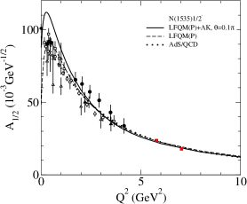
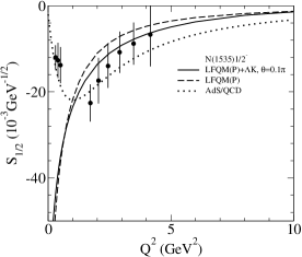
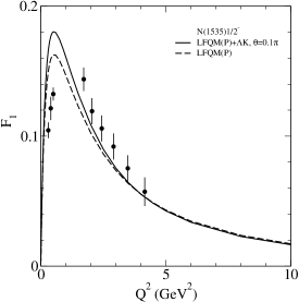
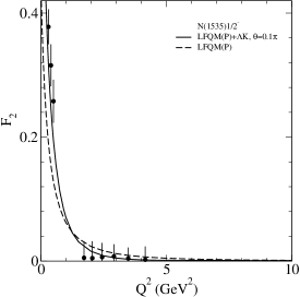
Figure 1: Helicity amplitudes and form factors of the $\gamma^{*}N\to N^{*}(1535)$ transition. CLAS data: circles (bold) Aznauryan:2009mx , squares (bold) Dalton2009 , triangle (bold) Armstrong2009 , circles (empty) Denizl2007 , triangles (empty) Burkert2003 , squares (empty) Thompson2001 , diamonds Dugger2009 . Theoretical description in terms of a light front (LF) quark model: dashed curves – results of calculations on the basis of three-quark configurations, $s^{2}p$ for the $N^{*}$ and $s^{3}$ for $N$, using a pole-like quark core wave function $\Phi_{0}$(denoted by LFQM(P) in the legends); solid curves – results for the model of Eq. (48) with the ”strong” value of mixing parameter $\cos\theta=\,$0.951 ($\theta=0.1\pi$); dotted curves – results of the soft-wall AdS/QCD model Gutsche:2019lyu .

Our results for the transition form factors and helicity amplitudes are shown in Figs. 1 and 2 in comparison with the high-quality data of the CLAS collaboration Aznauryan:2008pe ; Aznauryan:2009mx ; Mokeev:2015lda ; Park:2014yea ; Burkert:2016kyi ; Dalton2009 ; Armstrong2009 ; Denizl2007 ; Burkert2003 ; Thompson2001 ; Dugger2009 . We have used only three free parameters, $m,\beta$ and $\gamma$, in the wave function of quark core $\Phi_{0}$ of Eq. (25) in both cases the nucleon and the negative parity resonance. Here $m=m_{1}=m_{2}=m_{3}$ is the mass of a light constituent quark ($u,d$). In the case of the Roper resonance we also use two additional parameters, the coefficients $\alpha$ and $\beta_{1}$ of Eq. (26). The parameters $m,\beta$ and $\gamma$ are common to all the resonances. The parameter $c_{2}$ in the wave function of the radially excited quark core (24) is not free, since it is determined from the orthogonality condition $\langle\Phi_{0}|\Phi_{02}\rangle=\,$0. We neglect the quark anomalous magnetic moments ($\varkappa_{1}=\varkappa_{2}=\varkappa_{3}=\,$0) in the quark current defined in Eq. (16) as their values are too small ($\varkappa_{i}\lesssim\,$0.03, according to Ref. Obukhovsky:2013fpa ). The only influence they have is on the precise value of the baryon magnetic momentum. Parameters $m,\beta$ and $\gamma$ are taken from Refs. Schlumpf:1992ce ; Obukhovsky:2013fpa where they were fitted to the nucleon data in a large interval of 0$\leq Q^{2}\lesssim\,$32 GeV². Only the coefficients $\alpha$ and $\beta_{1}$ for a superposition of the Gaussian and the pole-like wave function of Eq. (26) has been varied to obtain the best description of the Roper resonance helicity amplitudes. In the end we obtain a decent description (Figs. 1 and 2) of form factors and helicity amplitudes of the three baryons (including the elastic nucleon form factors described in Ref. Obukhovsky:2013fpa ) at moderate/high momentum transfer, $Q^{2}\gtrsim\,$1-2 GeV², making use of the following values of parameters:

$$\beta=0.579\,\,{\rm GeV}\,,\quad\gamma=3.51,\quad m=0.251\,\,{\rm GeV}\,,\quad\alpha=0.245,\quad\beta_{1}=0.85\beta\,.$$ (49)

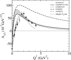
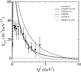
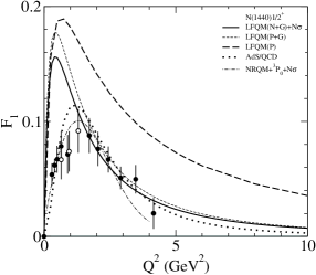
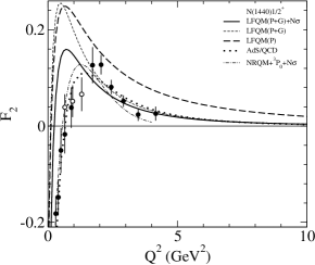
Figure 2: Helicity amplitudes and form factors of the $\gamma^{*}N\to N^{*}(1440)$ transition. Theoretical description in terms of a light front quark model (LFQM): dashed curves – results on the basis of three-quark configurations, $sp^{2}$ for the $N^{*}(1440)$ and $s^{3}$ for $N(940)$, using a pole-like quark core wave function $\Phi_{0}$; short dashed curves – results of calculations using a superposition given in Eq.(26) of pole-like function (P) and Gaussian (G) in the quark core wave function $\Phi_{0}^{R}$ with $\alpha=$0.245 (denoted by LFQM(P+G) in the legends); solid curves – results for the mixed-state model given in Eq. (48) with a ”strong” value of the mixing angle, $\cos\theta_{R}=\,$0.930 ($\theta_{R}=-0.12\pi$) (denoted by LFQM(P+G)+$N\sigma$ in the legends); dotted curves – results obtained in the soft-wall AdS/QCD approach Gutsche:2017lyu ; dashed-dotted curves – results for the nonrelativistic quark model (NRQM) with contributions of virtual $\bar{q}q$ pairs in terms of the ${}^{3}P_{0}$ model Obukhovsky:2011sc . The CLAS data (bold and empty circles) on one-pion Aznauryan:2009mx ; Aznauryan:2012ec and two-pion Mokeev:2015lda electroproduction off the proton. The A1 data on $\pi^{0}$ (the empty square) electroproduction Stajner:2017fmh .

Transition form factors and helicity amplitudes for the electroproduction of resonances of negative (Fig. 1) and positive (Fig. 2) parity calculated with a common for the nucleon and for the both resonances pole-like wave function $\Phi_{0}$ given in Eq. (25) are shown in Figs. 1 and 2 by dashed lines. In this case we neglect mixing of the pole-like wave function with the Gaussian for the Roper resonance and use the function (26) with the zero mixing ($\alpha=\,$1).The obtained results are close to the data in the case of $N_{1/2^{-}}(1535)$, but in the case of $N_{1/2^{+}}(1440)$ there are strong deviations. In the latter case one can improve the agreement by using a large mixing angle $\theta_{R}$ for the molecular state $N+\sigma$ in Eq. (48), taking e.g. $\cos{\theta_{R}}\simeq\sin{\theta_{R}}\approx\,$0.7 as we have done in our previous work Obukhovsky:2013fpa . However, the most realistic variant is a large mixing parameter for another (loose) quark configuration given in Eq. (26), (thin small-dashed lines in Fig. 2 which correspond to the value of $\alpha=\,$0.245). Then we obtain a good agreement with the data for the both resonances, $N_{1/2^{-}}(1535)$ and $N_{1/2^{+}}(1440)$, using small values of the mixing angle for the respective molecular states, $\cos{\tilde{\theta}}\simeq\cos{\theta_{R}}\simeq\,$0.93-0.95 (Figs. 1 and 2, solid lines). The shaded region in Fig. 2 (left upper panel) shows the range of the Roper helicity amplitude $A_{1/2}$ with the mixing angle changing from $\theta_{R}=0$ to $\theta_{R}=18^{0}$.

Our results demonstrate that the contribution of the hadron molecule to the transition amplitude quickly dies out with rising $Q^{2}$ and might be neglected at high $Q^{2}$. The contribution of the quark core correlates well with the data at $Q^{2}\gtrsim\,$1-2 GeV², if the parameter of mixing $\cos{\theta}$ is about 0.93-0.95. On this basis we predict the $Q^{2}$-behavior of amplitudes at high $Q^{2}\gtrsim\,$5-7 GeV² starting from the quark core wave function alone.

In the case of the Roper resonance there are discrepancies between the predictions of the model with the pole-like wave function $\Phi_{0}$ (dashed curves in Fig. 2) and the data. We have shown that one can considerably improve the agreement with data modifying only the quark core wave function by the replacement $\Phi_{0}\to\Phi_{9}^{R}$ following Eq. (26). This can be considered as an argument in support of the inner quark structure of the Roper resonance contrary to what might be expected from the above mentioned large discrepancies between predictions and data.

It is possible that in the case of the Roper resonance the unknown multiparticle component of the quark current plays a more important role than in the case of other resonances. It can be instructive to compare the results of our model (solid curves in Figs. 1 and 2) with a good description of the Roper resonance transition form factors recently obtained in Ref. Gutsche:2017lyu (dotted curves in Fig. 2) in a soft-wall AdS/QCD. The results of both LF models are close to each other (and close to the data) at $Q^{2}\gtrsim\,$1-2 GeV², but at low $Q^{2}$ the results of the LF quark model considerably differs from the AdS/QCD results which stay close to the CLAS data. This discrepancy can especially be traced to the strict requirement of orthogonality for the ground ($0S$) and excited ($2S$) radial wave functions of the $N$ and $R$ states belonging to quark configurations with the same spin-isospin ($S=\,$1/2, $T=1/2$) and symmetry ($[3]_{ST}[3]_{X}$) quantum numbers. Then, for the transition $N\to R$ (Roper), the matrix element of the single-particle current (16), which does not act on the orbital part of the wave function, should vanish for $Q^{2}\to 0$ (because of the orthogonality of the orbital parts of the baryon wave functions $\langle R_{orb}|N_{orb}\rangle=\,$0), as it really seen in Fig. 2 (solid and dashed curves are close to zero at $Q^{2}\to 0$). But the $A_{1/2}$ data at $Q^{2}\simeq 0$ are not small. Instead they cross the $Q^{2}$ axis at $Q^{2}\simeq 0.5$ GeV². The discrepancy of the quark model results and the data in this region can be an effect of multiparticle currents. We have modeled such an effect in our preceding work Obukhovsky:2011sc using a non-relativistic ${}^{3}P_{0}$ model for vacuum $\bar{q}q$ pairs. As a result we have obtained a realistic description of the amplitude $A_{1/2}$ at small values of $Q^{2}$ (dotted-dashed curves in Fig. 2). In the region of $Q^{2}\lesssim$1-2 GeV², where a non-relativistic quark model can be used reliably, such descriptions are very close to the CLAS data. In both cases of the $N\to N_{1/2^{+}}(1440)$ and $N\to N_{1/2^{-}}(1535)$ transitions AdS/QCD approach Gutsche:2017lyu ; Gutsche:2019lyu (dotted lines) gives very good discription of data and at large $Q^{2}$ it is very close to the the LF quark model results (solid lines). Note that successfull descrption of data in AdS/QCD approach in low energy domain is explained by inclusion of higher Fock states contribution into the structure of nucleon and nucleon resonances, while at high $Q^{2}$ it is provided by the correct power scaling of the form factors/helicity amplitudes consistent with quark counting rules. Summarizing the results shown in Figs. 1 and 2 it is worth noting that a good basis of quark configurations constructed at the light front, as performed in Sect. III-IV, might be an effective tool in the study of the inner structure of baryons. This is particularly true when the study is based on high-quality data on the baryon electroproduction at high momentum transfer.

Appendix A Canonical and front boosts for plain-wave states

The standard ”rotationless” Lorentz transformation $\Lambda(\frac{P}{M_{0}})$ which connects the momenta of a free particle in two different reference frames $p_{i}^{\mu}\to p_{i}^{\prime\mu}={\Lambda(\frac{P}{M_{0}})^{\mu}_{\nu}}p_{i}^{\nu}$ is denoted by index $c$ (canonical boost). The boosts $\Lambda_{c}$ are used in the case of the instant form of the dynamics. The respective canonical basis is defined Keister1991 ; Polyzou2013 as a basis of the unitary representation of the Poincaré group

$$\sqrt{\frac{\omega_{i}(\bm{p_{i}})}{m_{i}}}|(m_{i},s_{i});\bm{p}_{i},\mu_{i}\rangle_{Ó}=U[\Lambda_{c}(\frac{p_{i}}{m_{i}})]\,|(m_{i},s_{i});\bm{\stackrel{{\scriptstyle\circ}}{{p}}_{i}},\mu_{i}\rangle\,,\quad\bm{p}_{i}=\Lambda_{c}(\frac{p_{i}}{m_{i}})\bm{\stackrel{{\scriptstyle\circ}}{{p}}_{i}},$$ (50)

where $\stackrel{{\scriptstyle\circ}}{{p}}_{i}^{\mu}=\{m_{i},\bm{\stackrel{{\scriptstyle\circ}}{{p}}_{i}}\}$, $\bm{\stackrel{{\scriptstyle\circ}}{{p}}_{i}}=\bm{0}$. The factor $\sqrt{\frac{\omega_{i}(\bm{p_{i}})}{m_{i}}}$ follows from the standard normalization condition

$${}_{c\!}\langle\bm{p}_{i}^{\prime},\mu_{i}^{\prime}|\bm{p}_{i},\mu_{i}\rangle_{\!c}=(2\pi)^{3}\delta^{(3)}(\bm{p_{i}^{\prime}}-\bm{p_{i}})\,\delta_{\mu_{i}^{\prime}\mu_{i}}.$$ (51)

Apart from the canonical boost, the momenta $p_{i}^{\prime\mu}$ and $p_{i}^{\mu}$ can be connected by another element $G$ of the homogeneous Lorentz group. In particular, it might be the ”front boost” $\Lambda_{f}(\frac{\bm{\tilde{P}}}{M_{0}})$ with the respective front basis $|(m_{i},s_{i});\bm{\tilde{p}}_{i},\mu_{i}\rangle_{\!f}$, where $p_{i}^{\pm}=\omega_{i}(\bm{p}_{i})\pm p_{iz}$, and $\bm{\tilde{p}}_{i}:=\{p_{i}^{+},\bm{p}_{i\bot}\}$,

$$\sqrt{\frac{p_{i}^{+}}{m_{i}}}|(m_{i},s_{i});\bm{\tilde{p}}_{i},\mu_{i}\rangle_{\!f} = U[\Lambda_{f}(\frac{\tilde{p}_{i}}{m_{i}})]\,|(m_{i},s_{i});\bm{\stackrel{{\scriptstyle\circ}}{{p}}_{i}},\mu_{i}\rangle\,,\quad\bm{\tilde{p}}_{i}=\Lambda_{f}(\frac{\tilde{p}_{i}}{m_{i}})\bm{\stackrel{{\scriptstyle\circ}}{{p}}_{i}},$$

$${}_{f\!}\langle\bm{\tilde{p}}_{i}^{\prime},\mu_{i}^{\prime}|\bm{\tilde{p}}_{i},\mu_{i}\rangle_{\!f} = (2\pi)^{3}\delta^{(2)}(\bm{p_{i\bot}^{\prime}}-\bm{p_{i\bot}})\delta({p_{i}^{\prime}}^{+}-p_{i}^{+})\,\delta_{\mu_{i}^{\prime}\mu_{i}},$$ (52)

which are used in the front form of the dynamics. The matrices $\Lambda_{f}$ which connect the momenta $\tilde{p}_{i}^{\prime}$ and $\tilde{p}_{i}$, ${\tilde{p}}_{i}^{\prime\tilde{\mu}}={\Lambda_{f}(\frac{\tilde{P}}{M})}^{\tilde{\mu}}_{\tilde{\nu}}{\tilde{p}}_{i}^{\tilde{\nu}}$, are elements of the ”front subgroup” of the homogeneous Lorentz group. The light front $t-z=\,$0 is invariant under transformations of the front subgroup.

Canonical boosts $\Lambda_{Ó}(\frac{P}{M_{0}})$ itself do not form a subgroup of the Poincaré group, since the product of two boosts $\Lambda_{c}$ gives rise to the Wigner rotation $R_{w}$

$$\Lambda_{Ó}(\frac{P_{a}}{M})\Lambda_{Ó}(\frac{P_{b}}{M})=\Lambda_{Ó}(\frac{P}{M})R_{w}(\frac{P_{a}}{M},\frac{P_{b}}{M}),\quad P=\Lambda_{Ó}(\frac{P_{a}}{M})P_{b}\,,$$ (53)

while the product of front boosts does not give rise to the Wigner rotation,

$$\Lambda_{f}(\frac{\tilde{P}_{a}}{M})\Lambda_{f}(\frac{\tilde{P}_{b}}{M})=\Lambda_{f}(\frac{\tilde{P}}{M}),\quad\tilde{P}=\Lambda_{f}(\frac{\tilde{P}_{a}}{M})\tilde{P}_{b}\,.$$ (54)

Starting from Eqs. (50) and (53) and using the relationship $R\Lambda_{c}(\frac{p_{i}}{m_{i}})R^{-1}=\Lambda_{c}(\frac{Rp_{i}}{m_{i}})$ Keister1991 ; Polyzou2013 one readily obtains that the unitary irreducible representation of the canonical boost in the free basis (50) is of the form

$$U[\Lambda_{c}(\frac{P}{M_{0}})]\,|\bm{k}_{i},\mu_{i}\rangle_{\!c}=\sqrt{\frac{\omega_{i}(\bm{p}_{i})}{\omega_{i}(\bm{k}_{i})}}\sum_{\bar{\mu}_{i}}|R_{w}\bm{p}_{i},\bar{\mu}_{i}\rangle_{\!c}\,D^{(1/2)}_{\bar{\mu}_{i}\mu_{i}}(R_{w})\,,\quad\bm{p}_{i}=\Lambda_{c}(\frac{P}{M_{0}})\,\bm{k}_{i}\,,$$ (55)

where the arguments of the $D$ function are the Euler angles of the Wigner rotation (53). The unitary irreducible representation of the front boost is of a trivial form

$$U[\Lambda_{f}(\frac{\tilde{P}}{M_{0}})]\,|\bm{\tilde{k}}_{i},\mu_{i}\rangle_{\!f}=\sqrt{\frac{p_{i}^{+}}{k_{i}^{+}}}|\bm{\tilde{p}}_{i},\mu_{i}\rangle_{\!f}\,,\quad\bm{\tilde{p}}_{i}=\Lambda_{f}(\frac{\tilde{P}}{M_{0}})\,\bm{\tilde{k}}_{i}.$$ (56)

According to Eq. (56) the $z$ component of the front spin is a kinematical variable with the value of $\mu_{i}$ being constant at any transformation which leaves the light front $t-z=\,$0 invariant (including the spatial rotations around the $z$ axis). Therefore the $\mu_{i}$ can be identified with an additive quantum number, the helicity of the particle at the light front Chiu:2017ycx .

In Eqs. (55) and (56) the connection between the momenta $\bm{k}_{i}$ and $\bm{p}_{i}$ is symbolically written as $\bm{p}_{i}=\Lambda\,\bm{k}_{i}$. This implies the following $4\times 4$ matrices for boosts $\Lambda_{c}$ and $\Lambda_{f}$ Keister1991 ; Polyzou2013 :

$$p^{\mu}_{i}={\Lambda_{c}}^{\mu}_{\,\nu}\,k_{i}^{\nu}=\begin{pmatrix}\frac{P^{0}}{M_{0}}&\frac{\bm{P}}{M_{0}}\\ \frac{\bm{P}}{M_{0}}&\left(\delta_{ij}+\frac{P^{i}P^{j}}{M_{0}^{2}(1+\frac{P^{0}}{M_{0}})}\right)\end{pmatrix}\begin{pmatrix}\omega_{i}(\bm{k}_{i})\\ \bm{k}_{i}\end{pmatrix},\quad\mu(\nu)=0,1,2,3,$$ (57)

$$\tilde{p}^{\tilde{\mu}}_{i}={\Lambda_{f}}^{\tilde{\mu}}_{\,\tilde{\nu}}\,\tilde{k}_{i}^{\tilde{\nu}}=\begin{pmatrix}\frac{P^{+}}{M_{0}}&0&0\\ \frac{\bm{P_{\bot}}}{M_{0}}&1&0\\ \frac{\bm{P_{\bot}}^{2}}{M_{0}P^{+}}&\frac{2\bm{P_{\bot}}}{P^{+}}&\frac{M_{0}}{P^{+}}\end{pmatrix}\begin{pmatrix}k_{i}^{+}\\ \bm{k}_{i\bot}\\ k_{i}^{-}\end{pmatrix},\quad\tilde{\mu}(\tilde{\nu})=+,\bot,-.$$ (58)

The front boost (58) does not mix the ’kinematical component” ($\bm{\tilde{k}}_{i}\!=\!\{k_{i}^{+},\bm{k}_{i\bot}\}$) of momentum $\tilde{k}_{i}^{\tilde{\nu}}$ with its ”dynamical component” ($k_{i}^{-}=\frac{m_{i}^{2}+k_{i\bot}^{2}}{k_{i}^{+}}$), while the canonical boost (57) mixes the $\bm{k}_{i}$ and the $\omega_{i}(\bm{k}_{i})$. However in both cases the 3-momentum is an additive quantum number: $P_{12}^{+}=p_{1}^{+}+p_{2}^{+}$, $P^{+}=p_{1}^{+}+p_{2}^{+}+p_{3}^{+}$, $\bm{P}_{12\bot}=\bm{p}_{1\bot}+\bm{p}_{2\bot}$, $\dots$, etc. A similar property holds for the relative momenta, $\bm{\tilde{k}}=\Lambda^{-1}_{f}(\frac{\bm{\tilde{P}}_{12}}{m_{12}})\bm{\tilde{p}}_{1}$ and $\bm{\tilde{K}}\equiv\bm{\tilde{k}}_{3}=\Lambda^{-1}_{f}(\frac{\bm{\tilde{P}}}{M_{0}})\bm{\tilde{p}}_{3}$, which are connected with the momenta $\bm{\tilde{p}}_{i}$ by the linear relations

$$\bm{k}_{\bot}\!\!=\frac{x_{2}\bm{p}_{1\bot}\!-x_{1}\bm{p}_{2\bot}}{x_{1}+x_{2}},\,\,\bm{K}_{\bot}\!\!=\frac{(x_{1}\!+\!x_{2})\bm{p}_{3\bot}\!-x_{3}(\bm{p}_{1\bot}\!\!+\!\bm{p}_{2\bot})}{x_{1}+x_{2}+x_{3}},$$ (59)

$$k^{+}\!=\frac{m_{12}}{P_{12}^{+}}p_{1}^{+}\!=\!\frac{x_{1}}{x_{1}\!+x_{2}}m_{12},\quad K^{+}\!\equiv k_{3}^{+}\!=\frac{M_{0}}{P^{+}}p_{3}^{+}\!=\frac{x_{3}}{x_{1}+x_{2}+x_{3}}M_{0},$$ (60)

where

$$x_{i}=\frac{p_{i}^{+}}{P^{+}}=\frac{k_{i}^{+}}{M_{0}}.$$ (61)

These relations can be readily obtained by using the inverse of the matrices (58). Since $x_{1}+x_{2}+x_{3}=\,$1, only two independent parameters, $\xi$ and $\eta$, instead of $x_{1}=\xi\eta$, $x_{2}=(1\!-\!\xi)\eta$ and $x_{3}=1\!-\!\eta$ are used.

The important property of the variables (59) - (61) is that the values of $k_{\bot}\!\!=\!|\bm{k}_{\bot}|,\,K_{\bot}\!\!=\!|\bm{K}_{\bot}|$ and $x_{i}$ are relativistic invariants (it can be readily verified with the relations (58)) and the invariant masses $m_{12}$ and $M_{0}$ defined in Eq. (4) are functions only of $k_{\bot}$, $K_{\bot}$, $\xi$ and $\eta$,

$$m_{12}^{2}=\frac{k_{\bot}^{2}+m^{2}}{\xi(1-\xi)},\quad M_{0}^{2}=\frac{m_{12}^{2}}{\eta}+\frac{K_{\bot}^{2}+\eta m^{2}}{\eta(1-\eta)},\quad m_{1}=m_{2}=m_{3}=m.$$ (62)

In particular, one can use the function $M_{0}(k_{\bot},K_{\bot},\xi,\eta)$ as an argument of the relativistic wave function $\Phi^{LF}_{Mj}(M_{0})$ in Eq. (5) rewritten at the light front.

References

- (1) I. G. Aznauryan et al. (CLAS Collaboration), Phys. Rev. C 78, 045209 (2008)
- (2) I. G. Aznauryan et al. (CLAS Collaboration), Phys. Rev. C 80, 055203 (2009).
- (3) V. I. Mokeev et al., Phys. Rev. C 93, 025206 (2016).
- (4) K. Park et al. (CLAS Collaboration), Phys. Rev. C 91, 045203 (2015).
- (5) M. M. Dalton et al., Phys. Rev. C 80, 015205 (2009).
- (6) C. S. Armstrong et al., Phys. Rev. D 60, 052004 (2009).
- (7) H. Denizli et al., Phys. Rev, C 76, 015204 (2007).
- (8) V. D. Burkert et al., Phys. Rev. C 67, 035204 (2003).
- (9) R. Thompson et al., Phys. Rev. Lett. 86, 1702 (2001).
- (10) M. Dugger et al., Phys. Rev. C 79, 065206 (2009).
- (11) S. Stajner et al., Phys. Rev. Lett. 119, 022001 (2017).
- (12) V. D. Burkert (CLAS Collaboration), EPJ Web Conf. 134, 01001 (2017).
- (13) V. D. Burkert, Few Body Syst. 59, 57 (2018).
- (14) N. Isgur and G. Karl, Phys. Rev. D 18, 4187 (1978); Phys. Rev. D 19, 2653 (1979).
- (15) S. J. Brodsky, H. C. Pauli and S. S. Pinsky, Phys. Rept. 301, 299 (1998).
- (16) H. W. Lin, S. D. Cohen, R. G. Edwards and D. G. Richards, Phys. Rev. D 78, 114508 (2008); H. W. Lin and S. D. Cohen, AIP Conf. Proc. 1432, 305 (2012).
- (17) I. G. Aznauryan and V. D. Burkert, Phys. Rev. C 85, 055202 (2012),
- (18) I. T. Obukhovsky, A. Faessler, T. Gutsche, and V. E. Lyubovitskij, Phys. Rev. D 89, 014032 (2014).
- (19) I. G. Aznauryan et al., Int. J. Mod. Phys. E 22, 1330015 (2013).
- (20) G. Ramalho, Few Body Syst. 59, 92 (2018); Phys. Rev. D 95, 054008 (2017).
- (21) V. M. Braun et al., Phys. Rev. Lett. 103, 072001 (2009); I. V. Anikin, V. M. Braun, and N. Offen, Phys. Rev. D 92, 014018 (2015).
- (22) C. D. Roberts, Few Body Syst. 59, 72 (2018).
- (23) V. D. Burkert and C. D. Roberts, Rev. Mod. Phys. 91, 011003 (2019).
- (24) D. Jido, M. Doering, and E. Oset, Phys. Rev. C 77, 065207 (2008).
- (25) S. J. Brodsky and G. F. de Teramond, Phys. Rev. Lett. 96, 201601 (2006).
- (26) G. F. de Teramond and S. J. Brodsky, AIP Conf. Proc. 1432, 168 (2012).
- (27) S. J. Brodsky, G. F. de Teramond, H. G. Dosch and J. Erlich, Phys. Rept. 584, 1 (2015)
- (28) R. S. Sufian, G. F. de Teramond, S. J. Brodsky, A. Deur and H. G. Dosch, Phys. Rev. D 95, 014011 (2017).
- (29) T. Gutsche, V. E. Lyubovitskij, I. Schmidt, and A. Vega, Phys. Rev. D 87, 016017 (2013); Phys. Rev. D 86, 036007 (2012); Phys. Rev. D 85, 076003 (2012); A. Vega, I. Schmidt, T. Gutsche, and V. E. Lyubovitskij, Phys. Rev. D 83, 036001 (2011); A. Vega, I. Schmidt, T. Branz, T. Gutsche, and V. E. Lyubovitskij, Phys. Rev. D 80, 055014 (2009).
- (30) T. Gutsche, V. E. Lyubovitskij, I. Schmidt, and A. Vega, Phys. Rev. D 87, 016017 (2013).
- (31) G. Ramalho and D. Melnikov, Phys. Rev. D 97, 034037 (2018).
- (32) G. Ramalho, Phys. Rev. D 96, 054021 (2017).
- (33) T. Gutsche, V. E. Lyubovitskij, and I. Schmidt, Phys. Rev. D 97, 054011 (2018).
- (34) T. Gutsche, V. E. Lyubovitskij, and I. Schmidt, arXiv:1906.08641 [hep-ph].
- (35) T. Gutsche, V. E. Lyubovitskij, and I. Schmidt, in preparation.
- (36) P. A. M. Dirac, Rev. Mod. Phys. 21, 392 (1949).
- (37) I. G. Aznauryan, A. S. Bagdasaryan, N. L. Ter-Isakyan, Phys. Lett. 112B, 393 (1982); I. G. Aznauryan, Z. Phys. A 346, 297 (1993); Phys. Lett. B 316, 391 (1993).
- (38) H. J. Weber, Phys. Rev. D 41, 2201 (1990); Phys. Rev. C 41, 2783 (1990).
- (39) P. L. Chung and F. Coester, Phys. Rev. D 44, 229 (1991).
- (40) B. Julia-Diaz, D. O. Riska, and F. Coester, Phys. Rev. C 69, 035212 (2004) Phys. Rev. C 75, 069902(E) (2007) [hep-ph/0312169].
- (41) F. Cardarelli, E. Pace, G. Salme and S. Simula, Nucl. Phys. A 623, 361C (1997); F. Cardarelli, and S. Simula, Phys. Lett. B 467, 1 (1999).
- (42) F. Schlumpf, Mod. Phys. Lett. A 8, 2135 (1993); Zurich University doctoral thesis, RX-1421 (Zurich), hep-ph/9211255.
- (43) S. J. Brodsky and F. Schlumpf, Prog. Part. Nucl. Phys. 34, 69 (1995).
- (44) S. Capstick and B. D. Keister, Phys. Rev. D 51, 3598 (1995); S. Capstick, B. D. Keister and D. Morel, J. Phys. Conf. Ser. 69, 012016 (2007).
- (45) Iu. M. Shirokov, JETP 8, 703 (1959).
- (46) W. B. Berestetskii, M. V. Terent’ev, Sov. J. Nucl. Phys. 24, 547 (1976); 25, 653 (1977); 25, 347 (1977).
- (47) B. L. G. Bakker, L. A. Kondratyuk, M. V. Terent’ev, Nucl. Phys. B 158, 497 (1977).
- (48) L. A. Kondratyuk, M. V. Terent’ev, Sov. J. Nucl. Phys. 31, 561 (1980).
- (49) B. D Keister, W. N. Polyzou, Adv. Nucl. Phys. 209, 225 (1991).
- (50) W. N. Polyzou, W. Glockle, H. Witala. Few Body Syst. 54, 1667 (2013).
- (51) I. T. Obukhovsky, A. Faessler, D. K. Fedorov, T. Gutsche and V. E. Lyubovitskij, Phys. Rev. D 84, 014004 (2011).
- (52) E. Santopinto and M. M. Giannini, Phys. Rev. C 86, 065202 (2012)
- (53) M. Aiello, M. M. Giannini and E. Santopinto, J. Phys. G: Nucl. Part. Phys. 24, 753 (1998).
- (54) S. J. Brodsky and B. T. Chertok, Phys. Rev. D 14, 3003 (1976); S. J. Brodsky and G. R. Farrar, Phys. Rev. D 11, 1309 (1975).
- (55) B. Bakamjian, L. H. Thomas, Phys. Rev. 92, 1300 (1953).
- (56) H. J. Melosh, Phys. Rev. D 9, 1095 (1974).
- (57) K. Y. J. Chiu and S. J. Brodsky, Phys. Rev. D 95, 065035 (2017).
- (58) M. Hamermesh, Group Theory and its Application to Physical Problems, Addison-Wesley Publ. Cjmpany Inc. Reading, Massachusetts, 1964.
- (59) I. T. Obukhovsky, A. Faessler, T. Gutsche and V. E. Lyubovitskij, J. Phys. G 41, 095005 (2014).
- (60) M. Tanabashi et al. (Particle Data Group), Phys. Rev. D 98, 030001 (2018).
- (61) R. C. E. Devenish, T. S. Eisenschitz and J. G. Korner, Phys. Rev. D 14, 3063 (1976).
- (62) L. Tiator and M. Vanderhaegen, Phys. Lett. B 672, 344 (2009).
- (63) I. T. Obukhovsky, A. Faessler, T. Gutsche, D. K. Fedorov and V. E. Lyubovitskij, EPJ Web Conf. 138, 04003 (2017).
-
(64)
I. V. Anikin, M. A. Ivanov, N. B. Kulimanova and V. E. Lyubovitskij,
Z. Phys. C 65, 681 (1995);
M. A. Ivanov, M. P. Locher and V. E. Lyubovitskij, Few Body Syst. 21, 131 (1996) M. A. Ivanov, V. E. Lyubovitskij, J. G. Körner and P. Kroll, Phys. Rev. D 56, 348 (1997); A. Faessler, T. Gutsche, B. R. Holstein, M. A. Ivanov, J. G. Körner and V. E. Lyubovitskij, Phys. Rev. D 78, 094005 (2008); A. Faessler, T. Gutsche, M. A. Ivanov, J. G. Körner and V. E. Lyubovitskij, Phys. Rev. D 80, 034025 (2009); T. Branz, A. Faessler, T. Gutsche, M. A. Ivanov, J. G. Körner, V. E. Lyubovitskij and B. Oexl, Phys. Rev. D 81, 114036 (2010).