Schubert polynomials, pipe dreams, equivariant classes,
and a co-transition formula

Abstract.

We give a new proof that three families of polynomials coincide: the double Schubert polynomials of Lascoux and Schützenberger defined by divided difference operators, the pipe dream polynomials of Bergeron and Billey, and the equivariant cohomology classes of matrix Schubert varieties. All three families are shown to satisfy a “co-transition formula” which we explain to be some extent projectively dual to Lascoux’ transition formula. We comment on the $K$-theoretic extensions.

1. Overview

Let $S_{\infty}:=\cup_{n=1}^{\infty}S_{n}$ be the permutations $\pi$ of ${\mathbb{N}}_{+}$ that are eventually the identity, i.e. $\pi(i)=i$ for $i\gg 0$. We define three families of polynomials in $\mathbb{Z}[x_{1},x_{2},\ldots,y_{1},y_{2},\ldots]$, named $A$(lgebra), $C$(ombinatorics), and $G$(eometry), and each indexed by $S_{\infty}$:

1. Double Schubert polynomials $A_{\pi}$. These were defined by Lascoux and Schützenberger [La95], using a recurrence relation based on divided difference operators. We recapitulate the definition in §2, with a mildly novel approach.

2. Pipe dream polynomials $C_{\pi}$. These were introduced (in the $(x_{i})$ variables only, and not called this) by N. Bergeron and Billey [BeBi93]; we recall them in §3.

3. Matrix Schubert classes $G_{\pi}$. These were introduced by Fulton [Fu92, Fu99] (and again, not called this) to give universal formulæ for the classes of degeneracy loci of generic maps between flagged vector bundles. This concept was reinterpreted cohomologically in [KnMi05, Ka97], as giving the equivariant cohomology classes associated to matrix Schubert varieties; we recall this interpretation in §4.

In this paper we give an expeditious proof of the following known results [BeBi93, KnMi05]:

Theorem 1.1.

For all $\pi\in S_{\infty}$, $A_{\pi}=C_{\pi}=G_{\pi}$.

This will follow from a base case $w_{0}^{n}$ they share, where $w_{0}^{n}(i):=\begin{cases}i&\text{if }i>n\\ n+1-i&\text{if }i\leq n,\end{cases}$

Lemma (The base case).

For each of $P\in\{A,C,G\}$, we have $P_{w_{0}^{n}}=\displaystyle\prod_{i,j\in[n],\ i+j\leq n}(x_{i}-y_{j})$.

along with a recurrence they each enjoy:

Lemma (The co-transition formula).

For each of $P\in\{A,C,G\}$, and $\pi\in S_{n}\setminus\{w_{0}^{n}\}$, there exist $i$ such that $i+\pi(i)<n$. Pick $i$ minimum such. Then

$$(x_{i}-y_{\pi(i)})\,P_{\pi}=\sum\left\{P_{\sigma}\ :\ \sigma\in S_{n},\ \sigma\gtrdot\pi,\ \sigma(i)\neq\pi(i)\right\}$$

where $\gtrdot$ indicates a cover in the Bruhat order.

The derivations of the co-transition formula in the three families are to some extent parallel. For $P=A$ we define the “support” of a polynomial and remove one point from the support of $A_{\pi}$. In $P=C$ we (implicitly) study a subword complex [KnMi05] whose facets correspond to pipe dreams for $\pi$, and delete a cone vertex from the complex. In $P=G$ we study a hyperplane section of the matrix Schubert variety ${\overline{X}}_{\pi}$, which removes one $T$-fixed point from ${\overline{X}}_{\pi}/T$.

In the remainder we recall the polynomials and prove the lemmata for each of them. The word “transition” will appear in §2, but the “co-” will only be explained in §6. To further illuminate the connection between the pipe dream formula and the co-transition formula, we include in §5 an inductive formula that generalizes both and can be derived from either.

Acknowledgments.

It is a great pleasure to get to thank Bill for so much mathematics, encouragement, and guidance (especially in the practice and the importance of writing well; while my success has been limited I have at least always striven to emulate his example). I thank Ezra Miller for his many key insights in [KnMi05], even as I now obviate some of them here, and Bernd Sturmfels for his early input to that project. I thank the referee for catching some embarassing errors. Finally, this is my chance once more to thank Nantel Bergeron, Sara Billey, Sergei Fomin, and Anatol Kirillov for graciously accepting the terminology “pipe dream”. (See [BeCePi]!)

2. The double Schubert polynomials $(A_{\pi})$

Define the nil Hecke algebra $\mathbb{Z}[\partial]$ as having a $\mathbb{Z}$-basis $\{\partial_{\pi}\ :\ \pi\in S_{\infty}\}$ and the following very simple product structure:

$$\partial_{\pi}\partial_{\rho}:=\begin{cases}\partial_{\pi\circ\rho}&\text{if }\ell(\pi\rho)=\ell(\pi)+\ell(\rho)\\ 0&\text{otherwise, i.e. }\ell(\pi\rho)<\ell(\pi)+\ell(\rho).\end{cases}$$

Here $\ell(\pi):=\#\left\{(i,j)\in({\mathbb{N}}_{+})^{2}\ :\ i<j,\ \pi(i)>\pi(j)\right\}$ denotes the number of inversions of $\pi$. So this algebra $\mathbb{Z}[\partial]$ is graded by $\deg\partial_{\pi}=\ell(\pi)$, and plainly is generated by the degree $1$ elements $\{\partial_{i}:=\partial_{r_{i}}\}$, modulo the nil Hecke relations

$$\partial_{i}^{2}=0\qquad\qquad[\partial_{i},\partial_{j}]=0,\quad|i-j|>2\qquad\qquad\partial_{i}\partial_{i+1}\partial_{i}=\partial_{i+1}\partial_{i}\partial_{i+1}$$

This algebra has a module $\mathbb{Z}[{\underline{x}},{\underline{y}}]:=\mathbb{Z}[x_{1},x_{2},\ldots,y_{1},y_{2},\ldots]$ where the action is by divided difference operators in the $x$ variables:

$$\partial_{i}p:=\frac{p-r_{i}(p)}{x_{i}-x_{i+1}}$$

Here $r_{i}\circlearrowright\mathbb{Z}[{\underline{x}},{\underline{y}}]$ is the ring automorphism exchanging $x_{i}\leftrightarrow x_{i+1}$ and leaving all other variables alone. Since the numerator of $\partial_{i}p$ negates under switching $x_{i}$ and $x_{i+1}$, the long division algorithm for polynomials shows that numerator to be a multiple of $x_{i}-x_{i+1}$, so $\partial_{i}p$ is again a polynomial. To confirm that the above defines an action, one has to check the nil Hecke relations, which is straightforward.

The action is linear in the $(y_{i})$ variables, and the module comes with a $\mathbb{Z}[{\underline{y}}]$-linear augmentation $|_{e}:\,\mathbb{Z}[{\underline{x}},{\underline{y}}]\to\mathbb{Z}[{\underline{y}}]$ setting each $x_{i}\mapsto y_{i}$. With this, we can define a pairing

$$\mathbb{Z}[\partial]\times\mathbb{Z}[{\underline{x}},{\underline{y}}] \to \mathbb{Z}[{\underline{y}}]$$

$$(\partial_{w},p) \mapsto (\partial_{w}(p))\,|_{e}$$

Since the $\partial_{w}$ act $\mathbb{Z}[{\underline{y}}]$-linearly, it is safe to extend the scalars in the nil Hecke algebra from $\mathbb{Z}$ to $\mathbb{Z}[{\underline{y}}]$, and regard $\mathbb{Z}[{\underline{y}}]$ as our base ring for the two spaces being paired, as well as the target of their pairing.

Proposition 2.1.

This $\mathbb{Z}[{\underline{y}}]$-valued pairing of $\mathbb{Z}[{\underline{y}}][\partial]$ and $\mathbb{Z}[{\underline{x}},{\underline{y}}]$ is perfect, so the basis $\{\partial_{\pi}\ :\ \pi\in S_{\infty}\}$ has a dual $\mathbb{Z}[{\underline{y}}]$-basis $\{A_{\pi}\ :\ \pi\in S_{\infty}\}$ of $\mathbb{Z}[{\underline{x}},{\underline{y}}]$, called the double Schubert polynomials. These are homogeneous with $\deg(A_{\pi})=\ell(\pi)$.

In this basis, the $\mathbb{Z}[\partial]$-module structure becomes

$$\partial_{\pi}A_{\rho}=\begin{cases}A_{\rho\circ\pi^{-1}}&\text{if }\ell(\rho\circ\pi^{-1})=\ell(\rho)-\ell(\pi)\\ 0&\text{otherwise, i.e. if }\ell(\rho\circ\pi^{-1})>\ell(\rho)-\ell(\pi)\end{cases}$$

There are enough fine references for Schubert polynomials (e.g. [Fu96]) that we don’t further recapitulate the basics here. Dual bases are always unique, and perfection of the pairing is equivalent to existence of the dual basis. The usual proof of the existence starts with the base case $A_{w_{0}^{n}}$ as an axiom, defining the other double Schubert polynomials using the module action stated in the proposition.

It remains to prove the co-transition formula (for $P=A$), which in the “single” situation (setting all $y_{i}\equiv 0$) is plainly a Monk’s rule calculation. Since the “double” Monk rule is not a standard topic, and the references we found to it (e.g. notes by D. Anderson from a course by Fulton) use theory beyond the algebra definition above, we include a proof of the co-transition formula appropriate to $P=A$.

One tool for studying double Schubert polynomials is the $\mathbb{Z}[{\underline{y}}]$-algebra homomorphism $\mathbb{Z}[{\underline{x}},{\underline{y}}]\to\mathbb{Z}[{\underline{y}}]$, $x_{i}\mapsto y_{\rho(i)}\forall i$, called restriction to the point $\rho$. We’ll write this as $f\mapsto f|_{\rho}$, generalizing the case $\rho=e$ (the identity) we used above to define the pairing. Here is how it interacts with divided difference operators:

($$* (\partial_{i}f)|_{\rho}=\frac{f-r_{i}f}{x_{i}-x_{i+1}}\bigg{|}_{\rho}=\frac{f|_{\rho}-(r_{i}f)|_{\rho}}{x_{i}|_{\rho}-x_{i+1}|_{\rho}}=\frac{f|_{\rho}-f|_{\rho r_{i}}}{y_{\rho(i)}-y_{\rho(i+1)}}$$)

Define the support $supp(f)$ of a polynomial $f\in\mathbb{Z}[{\underline{x}},{\underline{y}}]$ by $supp(f):=\{\sigma\in S_{\infty}\ :\ f|_{\sigma}\neq 0\}$. It has a couple of obvious properties: $supp(pq)=supp(p)\cap supp(q)$, and $supp(p+q)\subseteq supp(p)\cup supp(q)$.

Proposition 2.2.

1. $supp(\partial_{i}f)\subseteq supp(f)\ \cup\ supp(f)\cdot r_{i}$

2. If $supp(f)\subseteq\{\tau:\tau\geq\sigma\}$, then $supp(\partial_{i}f)\subseteq\{\tau:\tau\geq\min(\sigma,\sigma r_{i})\}$.

3. $supp(A_{w_{0}^{n}})\cap S_{n}=\{w_{0}^{n}\}$

4. $A_{\pi}|_{\rho}=0$ unless $\rho\geq\pi$ in Bruhat order. (The converse holds, but we won’t show it.)

5. Let $\pi\in S_{n}$. Then $A_{\pi}|_{\pi}\neq 0$. (A small converse to (4).)

6. If $f|_{\rho}=0$ for all $\rho\in S_{\infty}$, then $f=0$.

7. There is an algorithm to expand a polynomial $p$ as a $\mathbb{Z}[{\underline{y}}]$-combination of double Schubert polynomials: look for a Bruhat-minimal element $\sigma$ of the support, subtract off $\frac{p|_{\sigma}}{A_{\sigma}|_{\sigma}}A_{\sigma}$ from $p$ (recording the coefficient $\frac{p|_{\sigma}}{A_{\sigma}|_{\sigma}}$), and recurse until $p$ becomes $0$.

Proof.

1. Use $(\partial_{i}f)|_{\rho}\ =\ f|_{\rho}/(y_{\rho(i)}-y_{\rho(i+1)})\ -\ f|_{\rho r_{i}}/(y_{\rho(i)}-y_{\rho(i+1)})$ from equation ($*$ ‣ 2).

2. This follows from (1) and the subword characterization of Bruhat order.

3. This follows trivially from $A_{w_{0}^{n}}=\prod_{i,j\in[n],\ i+j\leq n}(x_{i}-y_{j})$.

4. Fix $n$ such that $\pi,\rho\in S_{n}$, so $A_{\pi}=\partial_{\pi^{-1}w_{0}^{n}}A_{w_{0}^{n}}$. Let $Q$ be a reduced word for $\pi^{-1}w_{0}^{n}$. Apply (2); by the reducedness of $Q$ the $min(\sigma,\sigma r_{i})$ is always $\sigma r_{i}$. By induction on $\#Q$ we learn $supp(\partial_{\pi^{-1}w_{0}^{n}}A_{w_{0}^{n}})\subseteq\{\tau\ :\ \tau\geq\pi\}$, which is the result we seek.

5. We use downward induction in weak Bruhat order from the easy base case $w_{0}^{n}$. If $\pi r_{i}\gtrdot\pi$, then $A_{\pi}|_{\pi}=(\partial_{i}A_{\pi r_{i}})|_{\pi}\propto(A_{\pi r_{i}}|_{\pi}-A_{\pi r_{i}}|_{\pi r_{i}})=-A_{\pi r_{i}}|_{\pi r_{i}}\neq 0$ using equation ($*$ ‣ 2) for the $\propto$, part (4) to kill the first term, and induction.

6. Expand $f=\sum_{\pi\in S_{\infty}}c_{\pi}A_{\pi}$ in the $\mathbb{Z}[{\underline{y}}]$-basis $\{A_{\pi}\}$ and, if $f\neq 0$, let $A_{\rho}$ be a summand appearing (i.e. $c_{\rho}\neq 0$) with $\rho$ minimal in Bruhat order. Then $f|_{\rho}=\sum_{\pi}c_{\pi}A_{\pi}|_{\rho}=c_{\rho}A_{\rho}|_{\rho}$ by (4), and this is $\neq 0$ by (5).

7. In the finite $\mathbb{Z}[{\underline{y}}]$-expansion $p=\sum_{\rho}d_{\rho}A_{\rho}$, if $\sigma$ is chosen minimal such that $d_{\sigma}\neq 0$, then $p|_{\sigma}=\sum_{\rho}d_{\rho}A_{\rho}|_{\sigma}=d_{\sigma}A_{\sigma}|_{\sigma}\neq 0$, so $\sigma$ lies in $p$’s support. Meanwhile, by (4) $\sigma$ must also be Bruhat-minimal in $p$’s support. When we perform the subtraction in the algorithm, the coefficient is $d_{\sigma}$, and the number of terms in $p$ decreases.

∎

When we later learn $A=C=G$, then properties (4), (5) of the $(A_{\pi})$ will also hold for $(C_{\pi}),(G_{\pi})$, and we leave the reader to seek direct proofs of them.

Proposition 2.3 (Equivariant Monk’s rule).

Let $\pi\in S_{\infty}$, $i>0$. Then

$$(x_{i}-y_{\pi(i)})A_{\pi}=\sum_{\rho\gtrdot\pi}A_{\rho}\begin{cases}+1&\text{if }\rho(i)>\pi(i)\\ -1&\text{if }\rho(i)<\pi(i)\\ 0&\text{if }\rho(i)=\pi(i)\end{cases}$$

Proof.

Using the algorithm from proposition 2.2(7), and also proposition 2.2(4), we know that the expansion $f=\sum_{\rho}c_{\rho}A_{\rho}$ can only involve those $\rho\geq$ elements of $f$’s support. The support of $(x_{i}-y_{\pi(i)})A_{\pi}$ lies in $\{\rho\in S_{\infty}:\rho\geq\pi\}\setminus\{\pi\}=\{\rho\in S_{\infty}:\rho>\pi\}$. The only elements of that set with length $\leq\deg(x_{i}-y_{\pi(i)})A_{\pi}$ are $\{\rho\in S_{\infty}:\rho\gtrdot\pi\}$. Hence the left-hand side, expanded in double Schubert polynomials, must have constant coefficients, not higher-degree polynomials in $\mathbb{Z}[{\underline{y}}]$. (This is the sense in which the “right” extension of Monk’s nonequivariant rule concerns multiplication by $x_{i}-y_{\pi(i)}$ not just $x_{i}$. There is of course another, equally “right”, extension, computing $A_{r_{i}}A_{\pi}$.)

If a polynomial $f$ is in the common kernel of the $\partial_{j}$ operators, it must be symmetric in all the ${\underline{x}}$ variables… which means $f$ must involve no ${\underline{x}}$ variables at all, i.e. $f\in\mathbb{Z}[{\underline{y}}]$. If we also insist that $f|_{e}=0$ then we may infer $f=0$.

Both sides of our desired equation are homogeneous polynomials of the same degree, $\ell(\pi)+1$, and with $f|_{e}=0$. By the argument above it suffices to show that $\partial_{j}$ LHS $=\partial_{j}$ RHS for all $j$. There are five cases: $(j=i$ or $j=i-1)\times(\pi(i)>\pi(i+1)$ or $\pi(i)<\pi(i+1))$, and $j\neq i,i-1$, each of which one can check using the (itself easily checked) twisted Leibniz rule $\partial_{i}(fg)=(\partial_{i}f)g+(r_{i}f)(\partial_{i}g)$ along with induction on $\ell(\pi)$. We explicitly check the most unpleasant of the five cases: $j=i,\pi(i)>\pi(i+1)$.

$$\partial_{i}(x_{i}-y_{\pi(i)})A_{\pi} = A_{\pi}+(x_{i+1}-y_{\pi(i)})\partial_{i}A_{\pi}$$

$$= A_{\pi}+(x_{i+1}-y_{(\pi r_{i})(i+1)})A_{\pi r_{i}}\qquad\text{now use induction}$$

$$= A_{\pi}+\sum_{\sigma\gtrdot\pi r_{i}}A_{\sigma}\begin{cases}+1&\text{if }\sigma(i+1)>(\pi r_{i})(i+1)=\pi(i)\\ -1&\text{if }\sigma(i+1)<(\pi r_{i})(i+1)=\pi(i)\\ 0&\text{if }\sigma(i+1)=(\pi r_{i})(i+1)=\pi(i)\end{cases}$$

$$\sum_{\rho\gtrdot\pi}\partial_{i}A_{\rho}\begin{cases}+1&\text{if }\rho(i)>\pi(i)\\ -1&\text{if }\rho(i)<\pi(i)\\ 0&\text{if }\rho(i)=\pi(i)\end{cases} = \sum_{\rho\gtrdot\pi,\,\rho(i)>\rho(i+1)}A_{\rho r_{i}}\begin{cases}+1&\text{if }\rho(i)=(\rho r_{i})(i+1)>\pi(i)\\ -1&\text{if }\rho(i)=(\rho r_{i})(i+1)<\pi(i)\\ 0&\text{if }\rho(i)=(\rho r_{i})(i+1)=\pi(i)\end{cases}$$

Each term $\sigma$ in the first corresponds to the $\rho=\sigma r_{i}$ term in the second. ∎

Proof of the co-transition formula for $P=A$..

We need to check that each $\rho$ term in the equivariant Monk rule has $\rho(i)\in(\pi(i),n]$, so as to only get positive terms and only from $\rho\in S_{n}$.

Since $\pi$ has only descents before $i$ (by choice of $i$), we know $\rho=\pi\circ(i\leftrightarrow b)$ with $i<b$, i.e. $\rho(i)=\pi(b)>\pi(i)$.

By choice of $i$, we have $\pi=n\,n$-$1\ldots n$-$i$+$2\,\pi(i)\ldots\pi(n)$ with $\pi(i)<n-i+1$. Hence $\exists j\in(i,n]$ with $\pi(j)=n-i+1\in(\pi(i),n+1)$. The covering relations in $S_{\infty}$ don’t allow us to switch positions $i,n+k$ if some position $j\in(i,n+k)$ has $\pi(j)\in(\pi(i),\pi(n+k)=n+k)$. ∎

Lascoux’ transition formula [La01] for double Schubert polynomials is also based on Monk’s rule, but doesn’t include implicit division like the co-transition formula does. (It is worth noting that each of the summands on the right-hand side of the co-transition formula is divisible by $x_{i}-y_{\pi(i)}$, not merely their total.) We discuss the connection in §6.

3. The pipe dream polynomials $(C_{\pi})$

Index the squares in the Southeastern quadrant of the plane using matrix coordinates $\{(a,b)\ :\ a,b\in\{1,2,3,\ldots\}\}$. A pipe dream is a filling of that quadrant with two kinds of tiles, mostly     Π Υ            but finitely many           , such that no two pipes cross twice We label the pipes $1,2,3,\ldots$ across the top side, and speak of “the $1$-pipe of $D$”, “the $2$-pipe of $D$”, and so on. For example, the left two diagrams below are pipe dreams, the right one not:

$$\begin{array}[]{ccccc}&\hbox{\hbox to0.0pt{${\scriptstyle 1}$\hss}}\phantom{{\scriptstyle 1}}&\hbox{\hbox to0.0pt{${\scriptstyle 2}$\hss}}\phantom{{\scriptstyle 1}}&\hbox{\hbox to0.0pt{${\scriptstyle 3}$\hss}}\phantom{{\scriptstyle 1}}&\\ {\scriptstyle 1}&\smash{\raise 2.0pt\hbox{\co\hbox to0.0pt{\hbox to0.0pt{\char 5\relax\hss} \char 7\relax\hss}}\raise 6.0pt\hbox{\hbox to0.0pt{\vrule height=6.5pt\hss}}\raise 2.0pt\hbox{\hbox to0.0pt{\hskip 4.0pt\vrule height=0.4pt,depth=0.0pt,width=7.7pt\hss}}}&\smash{\lower 2.0pt\hbox{\hbox to0.0pt{\vrule height=14.0pt\hss}}\raise 2.0pt\hbox{\hbox to0.0pt{\hskip-3.0pt\vrule height=0.4pt,depth=0.0pt,width=14.7pt\hss}}}&\smash{\raise 2.0pt\hbox{\co\hbox to0.0pt{\hbox to0.0pt{\char 5\relax\hss} \char 7\relax\hss}}\raise 6.0pt\hbox{\hbox to0.0pt{\vrule height=6.5pt\hss}}\raise 2.0pt\hbox{\hbox to0.0pt{\hskip 4.0pt\vrule height=0.4pt,depth=0.0pt,width=7.7pt\hss}}}&\ \cdots\\ {\scriptstyle 3}&\smash{\raise 2.0pt\hbox{\co\hbox to0.0pt{\hbox to0.0pt{\char 5\relax\hss} \char 7\relax\hss}}\raise 6.0pt\hbox{\hbox to0.0pt{\vrule height=6.5pt\hss}}\raise 2.0pt\hbox{\hbox to0.0pt{\hskip 4.0pt\vrule height=0.4pt,depth=0.0pt,width=7.7pt\hss}}}&\smash{\raise 2.0pt\hbox{\co\hbox to0.0pt{\hbox to0.0pt{\char 5\relax\hss} \char 7\relax\hss}}\raise 6.0pt\hbox{\hbox to0.0pt{\vrule height=6.5pt\hss}}\raise 2.0pt\hbox{\hbox to0.0pt{\hskip 4.0pt\vrule height=0.4pt,depth=0.0pt,width=7.7pt\hss}}}&\smash{\raise 2.0pt\hbox{\co\hbox to0.0pt{\hbox to0.0pt{\char 5\relax\hss} \char 7\relax\hss}}\raise 6.0pt\hbox{\hbox to0.0pt{\vrule height=6.5pt\hss}}\raise 2.0pt\hbox{\hbox to0.0pt{\hskip 4.0pt\vrule height=0.4pt,depth=0.0pt,width=7.7pt\hss}}}\\ {\scriptstyle 2}&\smash{\raise 2.0pt\hbox{\co\hbox to0.0pt{\hbox to0.0pt{\char 5\relax\hss} \char 7\relax\hss}}\raise 6.0pt\hbox{\hbox to0.0pt{\vrule height=6.5pt\hss}}\raise 2.0pt\hbox{\hbox to0.0pt{\hskip 4.0pt\vrule height=0.4pt,depth=0.0pt,width=7.7pt\hss}}}&\smash{\raise 2.0pt\hbox{\co\hbox to0.0pt{\hbox to0.0pt{\char 5\relax\hss} \char 7\relax\hss}}\raise 6.0pt\hbox{\hbox to0.0pt{\vrule height=6.5pt\hss}}\raise 2.0pt\hbox{\hbox to0.0pt{\hskip 4.0pt\vrule height=0.4pt,depth=0.0pt,width=7.7pt\hss}}}&\smash{\raise 2.0pt\hbox{\co\hbox to0.0pt{\hbox to0.0pt{\char 5\relax\hss} \char 7\relax\hss}}\raise 6.0pt\hbox{\hbox to0.0pt{\vrule height=6.5pt\hss}}\raise 2.0pt\hbox{\hbox to0.0pt{\hskip 4.0pt\vrule height=0.4pt,depth=0.0pt,width=7.7pt\hss}}}\\ &\vdots&&&\ddots\end{array}\qquad\qquad\hbox{}\qquad\ \begin{array}[]{ccccc}&\hbox{\hbox to0.0pt{${\scriptstyle 1}$\hss}}\phantom{{\scriptstyle 1}}&\hbox{\hbox to0.0pt{${\scriptstyle 2}$\hss}}\phantom{{\scriptstyle 1}}&\hbox{\hbox to0.0pt{${\scriptstyle 3}$\hss}}\phantom{{\scriptstyle 1}}&\\ {\scriptstyle 1}&\smash{\raise 2.0pt\hbox{\co\hbox to0.0pt{\hbox to0.0pt{\char 5\relax\hss} \char 7\relax\hss}}\raise 6.0pt\hbox{\hbox to0.0pt{\vrule height=6.5pt\hss}}\raise 2.0pt\hbox{\hbox to0.0pt{\hskip 4.0pt\vrule height=0.4pt,depth=0.0pt,width=7.7pt\hss}}}&\smash{\raise 2.0pt\hbox{\co\hbox to0.0pt{\hbox to0.0pt{\char 5\relax\hss} \char 7\relax\hss}}\raise 6.0pt\hbox{\hbox to0.0pt{\vrule height=6.5pt\hss}}\raise 2.0pt\hbox{\hbox to0.0pt{\hskip 4.0pt\vrule height=0.4pt,depth=0.0pt,width=7.7pt\hss}}}&\smash{\raise 2.0pt\hbox{\co\hbox to0.0pt{\hbox to0.0pt{\char 5\relax\hss} \char 7\relax\hss}}\raise 6.0pt\hbox{\hbox to0.0pt{\vrule height=6.5pt\hss}}\raise 2.0pt\hbox{\hbox to0.0pt{\hskip 4.0pt\vrule height=0.4pt,depth=0.0pt,width=7.7pt\hss}}}&\ \cdots\\ {\scriptstyle 3}&\smash{\lower 2.0pt\hbox{\hbox to0.0pt{\vrule height=14.0pt\hss}}\raise 2.0pt\hbox{\hbox to0.0pt{\hskip-3.0pt\vrule height=0.4pt,depth=0.0pt,width=14.7pt\hss}}}&\smash{\raise 2.0pt\hbox{\co\hbox to0.0pt{\hbox to0.0pt{\char 5\relax\hss} \char 7\relax\hss}}\raise 6.0pt\hbox{\hbox to0.0pt{\vrule height=6.5pt\hss}}\raise 2.0pt\hbox{\hbox to0.0pt{\hskip 4.0pt\vrule height=0.4pt,depth=0.0pt,width=7.7pt\hss}}}&\smash{\raise 2.0pt\hbox{\co\hbox to0.0pt{\hbox to0.0pt{\char 5\relax\hss} \char 7\relax\hss}}\raise 6.0pt\hbox{\hbox to0.0pt{\vrule height=6.5pt\hss}}\raise 2.0pt\hbox{\hbox to0.0pt{\hskip 4.0pt\vrule height=0.4pt,depth=0.0pt,width=7.7pt\hss}}}\\ {\scriptstyle 2}&\smash{\raise 2.0pt\hbox{\co\hbox to0.0pt{\hbox to0.0pt{\char 5\relax\hss} \char 7\relax\hss}}\raise 6.0pt\hbox{\hbox to0.0pt{\vrule height=6.5pt\hss}}\raise 2.0pt\hbox{\hbox to0.0pt{\hskip 4.0pt\vrule height=0.4pt,depth=0.0pt,width=7.7pt\hss}}}&\smash{\raise 2.0pt\hbox{\co\hbox to0.0pt{\hbox to0.0pt{\char 5\relax\hss} \char 7\relax\hss}}\raise 6.0pt\hbox{\hbox to0.0pt{\vrule height=6.5pt\hss}}\raise 2.0pt\hbox{\hbox to0.0pt{\hskip 4.0pt\vrule height=0.4pt,depth=0.0pt,width=7.7pt\hss}}}&\smash{\raise 2.0pt\hbox{\co\hbox to0.0pt{\hbox to0.0pt{\char 5\relax\hss} \char 7\relax\hss}}\raise 6.0pt\hbox{\hbox to0.0pt{\vrule height=6.5pt\hss}}\raise 2.0pt\hbox{\hbox to0.0pt{\hskip 4.0pt\vrule height=0.4pt,depth=0.0pt,width=7.7pt\hss}}}\\ &\vdots&&&\ddots\end{array}\qquad\qquad\hbox{}\qquad\ \begin{array}[]{ccccc}&\hbox{\hbox to0.0pt{${\scriptstyle 1}$\hss}}\phantom{{\scriptstyle 1}}&\hbox{\hbox to0.0pt{${\scriptstyle 2}$\hss}}\phantom{{\scriptstyle 1}}&\hbox{\hbox to0.0pt{${\scriptstyle 3}$\hss}}\phantom{{\scriptstyle 1}}&\\ &\smash{\raise 2.0pt\hbox{\co\hbox to0.0pt{\hbox to0.0pt{\char 5\relax\hss} \char 7\relax\hss}}\raise 6.0pt\hbox{\hbox to0.0pt{\vrule height=6.5pt\hss}}\raise 2.0pt\hbox{\hbox to0.0pt{\hskip 4.0pt\vrule height=0.4pt,depth=0.0pt,width=7.7pt\hss}}}&\smash{\lower 2.0pt\hbox{\hbox to0.0pt{\vrule height=14.0pt\hss}}\raise 2.0pt\hbox{\hbox to0.0pt{\hskip-3.0pt\vrule height=0.4pt,depth=0.0pt,width=14.7pt\hss}}}&\smash{\raise 2.0pt\hbox{\co\hbox to0.0pt{\hbox to0.0pt{\char 5\relax\hss} \char 7\relax\hss}}\raise 6.0pt\hbox{\hbox to0.0pt{\vrule height=6.5pt\hss}}\raise 2.0pt\hbox{\hbox to0.0pt{\hskip 4.0pt\vrule height=0.4pt,depth=0.0pt,width=7.7pt\hss}}}&\ \cdots\\ &\smash{\lower 2.0pt\hbox{\hbox to0.0pt{\vrule height=14.0pt\hss}}\raise 2.0pt\hbox{\hbox to0.0pt{\hskip-3.0pt\vrule height=0.4pt,depth=0.0pt,width=14.7pt\hss}}}&\smash{\raise 2.0pt\hbox{\co\hbox to0.0pt{\hbox to0.0pt{\char 5\relax\hss} \char 7\relax\hss}}\raise 6.0pt\hbox{\hbox to0.0pt{\vrule height=6.5pt\hss}}\raise 2.0pt\hbox{\hbox to0.0pt{\hskip 4.0pt\vrule height=0.4pt,depth=0.0pt,width=7.7pt\hss}}}&\smash{\raise 2.0pt\hbox{\co\hbox to0.0pt{\hbox to0.0pt{\char 5\relax\hss} \char 7\relax\hss}}\raise 6.0pt\hbox{\hbox to0.0pt{\vrule height=6.5pt\hss}}\raise 2.0pt\hbox{\hbox to0.0pt{\hskip 4.0pt\vrule height=0.4pt,depth=0.0pt,width=7.7pt\hss}}}\\ &\smash{\raise 2.0pt\hbox{\co\hbox to0.0pt{\hbox to0.0pt{\char 5\relax\hss} \char 7\relax\hss}}\raise 6.0pt\hbox{\hbox to0.0pt{\vrule height=6.5pt\hss}}\raise 2.0pt\hbox{\hbox to0.0pt{\hskip 4.0pt\vrule height=0.4pt,depth=0.0pt,width=7.7pt\hss}}}&\smash{\raise 2.0pt\hbox{\co\hbox to0.0pt{\hbox to0.0pt{\char 5\relax\hss} \char 7\relax\hss}}\raise 6.0pt\hbox{\hbox to0.0pt{\vrule height=6.5pt\hss}}\raise 2.0pt\hbox{\hbox to0.0pt{\hskip 4.0pt\vrule height=0.4pt,depth=0.0pt,width=7.7pt\hss}}}&\smash{\raise 2.0pt\hbox{\co\hbox to0.0pt{\hbox to0.0pt{\char 5\relax\hss} \char 7\relax\hss}}\raise 6.0pt\hbox{\hbox to0.0pt{\vrule height=6.5pt\hss}}\raise 2.0pt\hbox{\hbox to0.0pt{\hskip 4.0pt\vrule height=0.4pt,depth=0.0pt,width=7.7pt\hss}}}\\ &\vdots&&&\ddots\end{array}$$

Because of the no-double-crossing rule, if we regard a pipe dream $D$ for $\pi$ as a wiring diagram for $\pi$, it’s easy to see that the number of            is exactly $\ell(\pi)$.

To a pipe dream $D$ we can associate a permutation $\pi$ by reading off the pipe labels down the left side, and say that $D$ is a “pipe dream for $\pi$”. With this we can define the pipe dream polynomials:

$$C_{\pi}:=\sum_{\text{pipe dreams $D$ for $\pi$}}\ \ \prod_{\text{crosses $+$ in $D$}}(x_{\text{row}(+)}-y_{\text{col}(+)})$$

$$\begin{matrix}\text{Example: }C_{1423}=&(x_{2}-y_{1})(x_{2}-y_{2})&+&(x_{2}-y_{1})(x_{1}-y_{3})&+&(x_{1}-y_{2})(x_{1}-y_{3})\\ &\begin{array}[]{ccccc}&\hbox{\hbox to0.0pt{${\scriptstyle 1}$\hss}}\phantom{{\scriptstyle 1}}&\hbox{\hbox to0.0pt{${\scriptstyle 2}$\hss}}\phantom{{\scriptstyle 1}}&\hbox{\hbox to0.0pt{${\scriptstyle 3}$\hss}}\phantom{{\scriptstyle 1}}&\hbox{\hbox to0.0pt{${\scriptstyle 4}$\hss}}\phantom{{\scriptstyle 1}}\\ {\scriptstyle 1}&\smash{\raise 2.0pt\hbox{\co\hbox to0.0pt{\hbox to0.0pt{\char 5\relax\hss} \char 7\relax\hss}}\raise 6.0pt\hbox{\hbox to0.0pt{\vrule height=6.5pt\hss}}\raise 2.0pt\hbox{\hbox to0.0pt{\hskip 4.0pt\vrule height=0.4pt,depth=0.0pt,width=7.7pt\hss}}}&\smash{\raise 2.0pt\hbox{\co\hbox to0.0pt{\hbox to0.0pt{\char 5\relax\hss} \char 7\relax\hss}}\raise 6.0pt\hbox{\hbox to0.0pt{\vrule height=6.5pt\hss}}\raise 2.0pt\hbox{\hbox to0.0pt{\hskip 4.0pt\vrule height=0.4pt,depth=0.0pt,width=7.7pt\hss}}}&\smash{\raise 2.0pt\hbox{\co\hbox to0.0pt{\hbox to0.0pt{\char 5\relax\hss} \char 7\relax\hss}}\raise 6.0pt\hbox{\hbox to0.0pt{\vrule height=6.5pt\hss}}\raise 2.0pt\hbox{\hbox to0.0pt{\hskip 4.0pt\vrule height=0.4pt,depth=0.0pt,width=7.7pt\hss}}}&\smash{\raise 2.0pt\hbox{\co\hbox to0.0pt{\hbox to0.0pt{\char 5\relax\hss} \phantom{\char 7\relax}\hss}}\raise 6.0pt\hbox{\hbox to0.0pt{\vrule height=6.0pt\hss}}}\\ {\scriptstyle 4}&\smash{\lower 2.0pt\hbox{\hbox to0.0pt{\vrule height=14.0pt\hss}}\raise 2.0pt\hbox{\hbox to0.0pt{\hskip-3.0pt\vrule height=0.4pt,depth=0.0pt,width=14.7pt\hss}}}&\smash{\lower 2.0pt\hbox{\hbox to0.0pt{\vrule height=14.0pt\hss}}\raise 2.0pt\hbox{\hbox to0.0pt{\hskip-3.0pt\vrule height=0.4pt,depth=0.0pt,width=14.7pt\hss}}}&\smash{\raise 2.0pt\hbox{\co\hbox to0.0pt{\hbox to0.0pt{\char 5\relax\hss} \phantom{\char 7\relax}\hss}}\raise 6.0pt\hbox{\hbox to0.0pt{\vrule height=6.0pt\hss}}}&\\ {\scriptstyle 2}&\smash{\raise 2.0pt\hbox{\co\hbox to0.0pt{\hbox to0.0pt{\char 5\relax\hss} \char 7\relax\hss}}\raise 6.0pt\hbox{\hbox to0.0pt{\vrule height=6.5pt\hss}}\raise 2.0pt\hbox{\hbox to0.0pt{\hskip 4.0pt\vrule height=0.4pt,depth=0.0pt,width=7.7pt\hss}}}&\smash{\raise 2.0pt\hbox{\co\hbox to0.0pt{\hbox to0.0pt{\char 5\relax\hss} \phantom{\char 7\relax}\hss}}\raise 6.0pt\hbox{\hbox to0.0pt{\vrule height=6.0pt\hss}}}&&\\ {\scriptstyle 3}&\smash{\raise 2.0pt\hbox{\co\hbox to0.0pt{\hbox to0.0pt{\char 5\relax\hss} \phantom{\char 7\relax}\hss}}\raise 6.0pt\hbox{\hbox to0.0pt{\vrule height=6.0pt\hss}}}&&&\\ \end{array}&&\begin{array}[]{ccccc}&\hbox{\hbox to0.0pt{${\scriptstyle 1}$\hss}}\phantom{{\scriptstyle 1}}&\hbox{\hbox to0.0pt{${\scriptstyle 2}$\hss}}\phantom{{\scriptstyle 1}}&\hbox{\hbox to0.0pt{${\scriptstyle 3}$\hss}}\phantom{{\scriptstyle 1}}&\hbox{\hbox to0.0pt{${\scriptstyle 4}$\hss}}\phantom{{\scriptstyle 1}}\\ {\scriptstyle 1}&\smash{\raise 2.0pt\hbox{\co\hbox to0.0pt{\hbox to0.0pt{\char 5\relax\hss} \char 7\relax\hss}}\raise 6.0pt\hbox{\hbox to0.0pt{\vrule height=6.5pt\hss}}\raise 2.0pt\hbox{\hbox to0.0pt{\hskip 4.0pt\vrule height=0.4pt,depth=0.0pt,width=7.7pt\hss}}}&\smash{\raise 2.0pt\hbox{\co\hbox to0.0pt{\hbox to0.0pt{\char 5\relax\hss} \char 7\relax\hss}}\raise 6.0pt\hbox{\hbox to0.0pt{\vrule height=6.5pt\hss}}\raise 2.0pt\hbox{\hbox to0.0pt{\hskip 4.0pt\vrule height=0.4pt,depth=0.0pt,width=7.7pt\hss}}}&\smash{\lower 2.0pt\hbox{\hbox to0.0pt{\vrule height=14.0pt\hss}}\raise 2.0pt\hbox{\hbox to0.0pt{\hskip-3.0pt\vrule height=0.4pt,depth=0.0pt,width=14.7pt\hss}}}&\smash{\raise 2.0pt\hbox{\co\hbox to0.0pt{\hbox to0.0pt{\char 5\relax\hss} \phantom{\char 7\relax}\hss}}\raise 6.0pt\hbox{\hbox to0.0pt{\vrule height=6.0pt\hss}}}\\ {\scriptstyle 4}&\smash{\lower 2.0pt\hbox{\hbox to0.0pt{\vrule height=14.0pt\hss}}\raise 2.0pt\hbox{\hbox to0.0pt{\hskip-3.0pt\vrule height=0.4pt,depth=0.0pt,width=14.7pt\hss}}}&\smash{\raise 2.0pt\hbox{\co\hbox to0.0pt{\hbox to0.0pt{\char 5\relax\hss} \char 7\relax\hss}}\raise 6.0pt\hbox{\hbox to0.0pt{\vrule height=6.5pt\hss}}\raise 2.0pt\hbox{\hbox to0.0pt{\hskip 4.0pt\vrule height=0.4pt,depth=0.0pt,width=7.7pt\hss}}}&\smash{\raise 2.0pt\hbox{\co\hbox to0.0pt{\hbox to0.0pt{\char 5\relax\hss} \phantom{\char 7\relax}\hss}}\raise 6.0pt\hbox{\hbox to0.0pt{\vrule height=6.0pt\hss}}}&\\ {\scriptstyle 2}&\smash{\raise 2.0pt\hbox{\co\hbox to0.0pt{\hbox to0.0pt{\char 5\relax\hss} \char 7\relax\hss}}\raise 6.0pt\hbox{\hbox to0.0pt{\vrule height=6.5pt\hss}}\raise 2.0pt\hbox{\hbox to0.0pt{\hskip 4.0pt\vrule height=0.4pt,depth=0.0pt,width=7.7pt\hss}}}&\smash{\raise 2.0pt\hbox{\co\hbox to0.0pt{\hbox to0.0pt{\char 5\relax\hss} \phantom{\char 7\relax}\hss}}\raise 6.0pt\hbox{\hbox to0.0pt{\vrule height=6.0pt\hss}}}&&\\ {\scriptstyle 3}&\smash{\raise 2.0pt\hbox{\co\hbox to0.0pt{\hbox to0.0pt{\char 5\relax\hss} \phantom{\char 7\relax}\hss}}\raise 6.0pt\hbox{\hbox to0.0pt{\vrule height=6.0pt\hss}}}&&&\\ \end{array}&&\begin{array}[]{ccccc}&\hbox{\hbox to0.0pt{${\scriptstyle 1}$\hss}}\phantom{{\scriptstyle 1}}&\hbox{\hbox to0.0pt{${\scriptstyle 2}$\hss}}\phantom{{\scriptstyle 1}}&\hbox{\hbox to0.0pt{${\scriptstyle 3}$\hss}}\phantom{{\scriptstyle 1}}&\hbox{\hbox to0.0pt{${\scriptstyle 4}$\hss}}\phantom{{\scriptstyle 1}}\\ {\scriptstyle 1}&\smash{\raise 2.0pt\hbox{\co\hbox to0.0pt{\hbox to0.0pt{\char 5\relax\hss} \char 7\relax\hss}}\raise 6.0pt\hbox{\hbox to0.0pt{\vrule height=6.5pt\hss}}\raise 2.0pt\hbox{\hbox to0.0pt{\hskip 4.0pt\vrule height=0.4pt,depth=0.0pt,width=7.7pt\hss}}}&\smash{\lower 2.0pt\hbox{\hbox to0.0pt{\vrule height=14.0pt\hss}}\raise 2.0pt\hbox{\hbox to0.0pt{\hskip-3.0pt\vrule height=0.4pt,depth=0.0pt,width=14.7pt\hss}}}&\smash{\lower 2.0pt\hbox{\hbox to0.0pt{\vrule height=14.0pt\hss}}\raise 2.0pt\hbox{\hbox to0.0pt{\hskip-3.0pt\vrule height=0.4pt,depth=0.0pt,width=14.7pt\hss}}}&\smash{\raise 2.0pt\hbox{\co\hbox to0.0pt{\hbox to0.0pt{\char 5\relax\hss} \phantom{\char 7\relax}\hss}}\raise 6.0pt\hbox{\hbox to0.0pt{\vrule height=6.0pt\hss}}}\\ {\scriptstyle 4}&\smash{\raise 2.0pt\hbox{\co\hbox to0.0pt{\hbox to0.0pt{\char 5\relax\hss} \char 7\relax\hss}}\raise 6.0pt\hbox{\hbox to0.0pt{\vrule height=6.5pt\hss}}\raise 2.0pt\hbox{\hbox to0.0pt{\hskip 4.0pt\vrule height=0.4pt,depth=0.0pt,width=7.7pt\hss}}}&\smash{\raise 2.0pt\hbox{\co\hbox to0.0pt{\hbox to0.0pt{\char 5\relax\hss} \char 7\relax\hss}}\raise 6.0pt\hbox{\hbox to0.0pt{\vrule height=6.5pt\hss}}\raise 2.0pt\hbox{\hbox to0.0pt{\hskip 4.0pt\vrule height=0.4pt,depth=0.0pt,width=7.7pt\hss}}}&\smash{\raise 2.0pt\hbox{\co\hbox to0.0pt{\hbox to0.0pt{\char 5\relax\hss} \phantom{\char 7\relax}\hss}}\raise 6.0pt\hbox{\hbox to0.0pt{\vrule height=6.0pt\hss}}}&\\ {\scriptstyle 2}&\smash{\raise 2.0pt\hbox{\co\hbox to0.0pt{\hbox to0.0pt{\char 5\relax\hss} \char 7\relax\hss}}\raise 6.0pt\hbox{\hbox to0.0pt{\vrule height=6.5pt\hss}}\raise 2.0pt\hbox{\hbox to0.0pt{\hskip 4.0pt\vrule height=0.4pt,depth=0.0pt,width=7.7pt\hss}}}&\smash{\raise 2.0pt\hbox{\co\hbox to0.0pt{\hbox to0.0pt{\char 5\relax\hss} \phantom{\char 7\relax}\hss}}\raise 6.0pt\hbox{\hbox to0.0pt{\vrule height=6.0pt\hss}}}&&\\ {\scriptstyle 3}&\smash{\raise 2.0pt\hbox{\co\hbox to0.0pt{\hbox to0.0pt{\char 5\relax\hss} \phantom{\char 7\relax}\hss}}\raise 6.0pt\hbox{\hbox to0.0pt{\vrule height=6.0pt\hss}}}&&&\\ \end{array}\end{matrix}$$

where we skip drawing any of the pipes outside the triangle $\{(a,b)\ :\ a+b\leq n\}$, as will be justified by lemma 3.1 below.

The main idea of the proof of the co-transition formula for the $\{C_{w}\}$ polynomials is easy to explain. Let ${\mathcal{D}}_{1}$ be the set of pipe dreams for $w$, and

$${\mathcal{D}}_{2}:=\bigcup\ \{\text{the pipe dreams for }w^{\prime}\ :\ w^{\prime}\text{ occurs in the co-transition formula}\}.$$

Our goal (which will take some doing) is to show that the maps

$$\begin{array}[]{rclcrclr}\qquad\qquad{\mathcal{D}}_{1}&\to&{\mathcal{D}}_{2}&&{\mathcal{D}}_{2}&\to&{\mathcal{D}}_{1}&\\ D\ \hskip 0.1pt\smash{\raise 2.8pt\hbox{\co\hskip 4.15pt\hbox to0.0pt{\hbox to0.0pt{\char 5\relax\hss} \char 7\relax\hss} \lower 6.8pt\hbox to0.0pt{\vrule height=3.5pt\hss} \raise 3.6pt\hbox to0.0pt{\vrule height=3.5pt\hss}}\raise 2.8pt\hbox{\hbox to0.0pt{\hskip-7.15pt\vrule height=0.4pt,depth=0.0pt,width=3.5pt\hss}\hbox to0.0pt{\hskip 4.05pt\vrule height=0.4pt,depth=0.0pt,width=3.5pt\hss}}}\hskip 8.7pt&\mapsto&D\ \smash{\lower 4.0pt\hbox{\hbox to0.0pt{\hskip 4.15pt\vrule height=14.0pt\hss}}\raise 2.8pt\hbox{\hbox to0.0pt{\hskip-3.0pt\vrule height=0.4pt,depth=0.0pt,width=14.7pt\hss}}}\hskip 12.7pt&&D\ \smash{\lower 4.0pt\hbox{\hbox to0.0pt{\hskip 4.15pt\vrule height=14.0pt\hss}}\raise 2.8pt\hbox{\hbox to0.0pt{\hskip-3.0pt\vrule height=0.4pt,depth=0.0pt,width=14.7pt\hss}}}\hskip 12.7pt&\mapsto&D\ \hskip 0.1pt\smash{\raise 2.8pt\hbox{\co\hskip 4.15pt\hbox to0.0pt{\hbox to0.0pt{\char 5\relax\hss} \char 7\relax\hss} \lower 6.8pt\hbox to0.0pt{\vrule height=3.5pt\hss} \raise 3.6pt\hbox to0.0pt{\vrule height=3.5pt\hss}}\raise 2.8pt\hbox{\hbox to0.0pt{\hskip-7.15pt\vrule height=0.4pt,depth=0.0pt,width=3.5pt\hss}\hbox to0.0pt{\hskip 4.05pt\vrule height=0.4pt,depth=0.0pt,width=3.5pt\hss}}}\hskip 8.7pt&\end{array}$$

that place, or remove, a            at position $(i,\pi(i))$ have the claimed targets ${\mathcal{D}}_{2}$, ${\mathcal{D}}_{1}$. The maps are then obviously inverse, and the co-transition formula will follow easily.

Lemma 3.1.

Let $w\in{S_{{\mathbb{N}}}}$, and $i\in\{1,2,\ldots\}$ such that $\forall j\in\{1,2,\ldots\},$ $i<j\iff w(i)<w(j)$. Then the pipe that enters from the North in column $i$ only goes through     Π Υ            tiles, no           , coming out at row $w(i)$. Consequently, if $w\in{S_{n}}$ and $D$ is a pipe dream for $w$, then there are no            tiles outside the triangle $\{(a,b)\ :\ a+b\leq n\}$.

Proof.

If $i<j$ and $w(i)<w(j)$, then the $i$-pipe starts and ends Northwest of the $j$-pipe. By the Jordan curve theorem these two pipes cross an even number of times, and since $D$ is a pipe dream, that even number is $0$. The opposite argument (Southeast) works if $i>j$ and $w(i)>w(j)$. Doing this for all $j\neq i$, we find that the $i$-pipe crosses no other pipe, i.e. it goes only through     Π Υ            tiles, ruling out            tiles in the adjacent diagonals $\{(a,b)\ :\ a+b=i-1,i\}$. Finally, if $w\in{S_{n}}$ then each $i>n$ satisfies the condition. ∎

Proof of the base case for $P=C$..

The number of squares in the triangle $\{(a,b)\ :\ a+b\leq n\}$ is $n\choose 2$, which is also $\ell(w_{0}^{n})$. As such, every one of them must have a            in a pipe dream for $w_{0}^{n}$, making the pipe dream for $w_{0}^{n}$ unique. Then the definition of $C_{\pi}$ gives the base case. ∎

Lemma 3.2.

Let $\pi,i,\rho$ be as in the co-transition formula. If $D$ is a pipe dream for $\pi$, then the leftmost     Π Υ            in rows $1,2,\ldots,i$ of $D$ occurs in column $\pi(1),\pi(2),\ldots,\pi(i)$ respectively. If $D^{\prime}$ is a pipe dream for $\rho$, then the same is true in rows $1,2,\ldots,i-1$ but in row $i$ the leftmost     Π Υ            occurs strictly to the right of column $\pi(i)$.

Proof.

Assume that the claim is established for each row above the $j$th. Start on the North side of $D$ in column $\pi(j)$, and follow that pipe down. By our inductive knowledge of rows $1\ldots j-1$, and the fact that $\pi(1)>\pi(2)>\cdots>\pi(i)$ by choice of $i$, this pipe will go straight down through $j-1$ crosses to the $j$th row. Since it then needs to exit on the $j$th row, it must turn West in matrix position $(j,\pi(j))$, and go due West through only            in columns $1,\ldots,\pi(j)-1$ of that row.

Exactly the same analysis holds for $\rho$, except that $\rho(i)>\pi(i)$. ∎

The following technical lemma is key.

Lemma 3.3.

Let $D$ be a filling of the Southeastern quadrant with finitely many           , the rest     Π Υ           , except with an empty square at $(a,b)$. Let $N$, $S$, $E$, $W$ denote the four pipes coming out of $(a,b)$ in those respective compass directions and call the remaining pipes the “old pipes”. Let $D\ \hskip 0.1pt\smash{\raise 2.8pt\hbox{\co\hskip 4.15pt\hbox to0.0pt{\hbox to0.0pt{\char 5\relax\hss} \char 7\relax\hss} \lower 6.8pt\hbox to0.0pt{\vrule height=3.5pt\hss} \raise 3.6pt\hbox to0.0pt{\vrule height=3.5pt\hss}}\raise 2.8pt\hbox{\hbox to0.0pt{\hskip-7.15pt\vrule height=0.4pt,depth=0.0pt,width=3.5pt\hss}\hbox to0.0pt{\hskip 4.05pt\vrule height=0.4pt,depth=0.0pt,width=3.5pt\hss}}}\hskip 8.7pt$, $D\ \smash{\lower 4.0pt\hbox{\hbox to0.0pt{\hskip 4.15pt\vrule height=14.0pt\hss}}\raise 2.8pt\hbox{\hbox to0.0pt{\hskip-3.0pt\vrule height=0.4pt,depth=0.0pt,width=14.7pt\hss}}}\hskip 12.7pt$ denote $D$ with the respective tile inserted at $(a,b)$; these have “new pipes” $WN,ES$ in $D\ \hskip 0.1pt\smash{\raise 2.8pt\hbox{\co\hskip 4.15pt\hbox to0.0pt{\hbox to0.0pt{\char 5\relax\hss} \char 7\relax\hss} \lower 6.8pt\hbox to0.0pt{\vrule height=3.5pt\hss} \raise 3.6pt\hbox to0.0pt{\vrule height=3.5pt\hss}}\raise 2.8pt\hbox{\hbox to0.0pt{\hskip-7.15pt\vrule height=0.4pt,depth=0.0pt,width=3.5pt\hss}\hbox to0.0pt{\hskip 4.05pt\vrule height=0.4pt,depth=0.0pt,width=3.5pt\hss}}}\hskip 8.7pt$ and $NS,EW$ in $D\ \smash{\lower 4.0pt\hbox{\hbox to0.0pt{\hskip 4.15pt\vrule height=14.0pt\hss}}\raise 2.8pt\hbox{\hbox to0.0pt{\hskip-3.0pt\vrule height=0.4pt,depth=0.0pt,width=14.7pt\hss}}}\hskip 12.7pt$. Assume that:

1. Every square West of $E$ except the hole $(a,b)$ (so, in rows $1,\ldots,a$) has a           , so in particular, the pipes $N$ and $W$ are straight.

Then if $D\ \hskip 0.1pt\smash{\raise 2.8pt\hbox{\co\hskip 4.15pt\hbox to0.0pt{\hbox to0.0pt{\char 5\relax\hss} \char 7\relax\hss} \lower 6.8pt\hbox to0.0pt{\vrule height=3.5pt\hss} \raise 3.6pt\hbox to0.0pt{\vrule height=3.5pt\hss}}\raise 2.8pt\hbox{\hbox to0.0pt{\hskip-7.15pt\vrule height=0.4pt,depth=0.0pt,width=3.5pt\hss}\hbox to0.0pt{\hskip 4.05pt\vrule height=0.4pt,depth=0.0pt,width=3.5pt\hss}}}\hskip 8.7pt$, is a pipe dream, so is $D\ \smash{\lower 4.0pt\hbox{\hbox to0.0pt{\hskip 4.15pt\vrule height=14.0pt\hss}}\raise 2.8pt\hbox{\hbox to0.0pt{\hskip-3.0pt\vrule height=0.4pt,depth=0.0pt,width=14.7pt\hss}}}\hskip 12.7pt$. If in addition we assume

1. No old pipe has North end between $N$ and $E$’s North ends while also having West end between $W$ and $S$’s West ends

then $D\ \smash{\lower 4.0pt\hbox{\hbox to0.0pt{\hskip 4.15pt\vrule height=14.0pt\hss}}\raise 2.8pt\hbox{\hbox to0.0pt{\hskip-3.0pt\vrule height=0.4pt,depth=0.0pt,width=14.7pt\hss}}}\hskip 12.7pt$ being a pipe dream implies $D\ \hskip 0.1pt\smash{\raise 2.8pt\hbox{\co\hskip 4.15pt\hbox to0.0pt{\hbox to0.0pt{\char 5\relax\hss} \char 7\relax\hss} \lower 6.8pt\hbox to0.0pt{\vrule height=3.5pt\hss} \raise 3.6pt\hbox to0.0pt{\vrule height=3.5pt\hss}}\raise 2.8pt\hbox{\hbox to0.0pt{\hskip-7.15pt\vrule height=0.4pt,depth=0.0pt,width=3.5pt\hss}\hbox to0.0pt{\hskip 4.05pt\vrule height=0.4pt,depth=0.0pt,width=3.5pt\hss}}}\hskip 8.7pt$ is a pipe dream.

We give an example to refer to while following the case analysis in the proof.

$$D\ \hskip 0.1pt\smash{\raise 2.8pt\hbox{\co\hskip 4.15pt\hbox to0.0pt{\hbox to0.0pt{\char 5\relax\hss} \char 7\relax\hss} \lower 6.8pt\hbox to0.0pt{\vrule height=3.5pt\hss} \raise 3.6pt\hbox to0.0pt{\vrule height=3.5pt\hss}}\raise 2.8pt\hbox{\hbox to0.0pt{\hskip-7.15pt\vrule height=0.4pt,depth=0.0pt,width=3.5pt\hss}\hbox to0.0pt{\hskip 4.05pt\vrule height=0.4pt,depth=0.0pt,width=3.5pt\hss}}}\hskip 8.7pt=\begin{array}[]{cccccccc}&&&\hbox{\hbox to0.0pt{${\scriptstyle WN}$\hss}}\phantom{{\scriptstyle 1}}&&\hbox{\hbox to0.0pt{${\scriptstyle ES}$\hss}}\phantom{{\scriptstyle 1}}\\ &&\hbox{\hbox to0.0pt{${\scriptstyle 1}$\hss}}\phantom{{\scriptstyle 1}}&\hbox{\hbox to0.0pt{${\scriptstyle 2}$\hss}}\phantom{{\scriptstyle 1}}&\hbox{\hbox to0.0pt{${\scriptstyle 3}$\hss}}\phantom{{\scriptstyle 1}}&\hbox{\hbox to0.0pt{${\scriptstyle 4}$\hss}}\phantom{{\scriptstyle 1}}&\hbox{\hbox to0.0pt{${\scriptstyle 5}$\hss}}\phantom{{\scriptstyle 1}}&\hbox{\hbox to0.0pt{${\scriptstyle 6}$\hss}}\phantom{{\scriptstyle 1}}\\ &{\scriptstyle 6}&\smash{\lower 2.0pt\hbox{\hbox to0.0pt{\vrule height=14.0pt\hss}}\raise 2.0pt\hbox{\hbox to0.0pt{\hskip-3.0pt\vrule height=0.4pt,depth=0.0pt,width=14.7pt\hss}}}&\smash{\lower 2.0pt\hbox{\hbox to0.0pt{\vrule height=14.0pt\hss}}\raise 2.0pt\hbox{\hbox to0.0pt{\hskip-3.0pt\vrule height=0.4pt,depth=0.0pt,width=14.7pt\hss}}}&\smash{\lower 2.0pt\hbox{\hbox to0.0pt{\vrule height=14.0pt\hss}}\raise 2.0pt\hbox{\hbox to0.0pt{\hskip-3.0pt\vrule height=0.4pt,depth=0.0pt,width=14.7pt\hss}}}&\smash{\lower 2.0pt\hbox{\hbox to0.0pt{\vrule height=14.0pt\hss}}\raise 2.0pt\hbox{\hbox to0.0pt{\hskip-3.0pt\vrule height=0.4pt,depth=0.0pt,width=14.7pt\hss}}}&\smash{\lower 2.0pt\hbox{\hbox to0.0pt{\vrule height=14.0pt\hss}}\raise 2.0pt\hbox{\hbox to0.0pt{\hskip-3.0pt\vrule height=0.4pt,depth=0.0pt,width=14.7pt\hss}}}&\smash{\raise 2.0pt\hbox{\co\hbox to0.0pt{\hbox to0.0pt{\char 5\relax\hss} \phantom{\char 7\relax}\hss}}\raise 6.0pt\hbox{\hbox to0.0pt{\vrule height=6.0pt\hss}}}\\ {\scriptstyle WN}&{\scriptstyle 2}&\smash{\lower 2.0pt\hbox{\hbox to0.0pt{\vrule height=14.0pt\hss}}\raise 2.0pt\hbox{\hbox to0.0pt{\hskip-3.0pt\vrule height=0.4pt,depth=0.0pt,width=14.7pt\hss}}}&\smash{\raise 2.0pt\hbox{\co\hbox to0.0pt{\hbox to0.0pt{\char 5\relax\hss} \char 7\relax\hss}}\raise 6.0pt\hbox{\hbox to0.0pt{\vrule height=6.5pt\hss}}\raise 2.0pt\hbox{\hbox to0.0pt{\hskip 4.0pt\vrule height=0.4pt,depth=0.0pt,width=7.7pt\hss}}}&\smash{\lower 2.0pt\hbox{\hbox to0.0pt{\vrule height=14.0pt\hss}}\raise 2.0pt\hbox{\hbox to0.0pt{\hskip-3.0pt\vrule height=0.4pt,depth=0.0pt,width=14.7pt\hss}}}&\smash{\raise 2.0pt\hbox{\co\hbox to0.0pt{\hbox to0.0pt{\char 5\relax\hss} \char 7\relax\hss}}\raise 6.0pt\hbox{\hbox to0.0pt{\vrule height=6.5pt\hss}}\raise 2.0pt\hbox{\hbox to0.0pt{\hskip 4.0pt\vrule height=0.4pt,depth=0.0pt,width=7.7pt\hss}}}&\smash{\raise 2.0pt\hbox{\co\hbox to0.0pt{\hbox to0.0pt{\char 5\relax\hss} \phantom{\char 7\relax}\hss}}\raise 6.0pt\hbox{\hbox to0.0pt{\vrule height=6.0pt\hss}}}\\ &{\scriptstyle 1}&\smash{\raise 2.0pt\hbox{\co\hbox to0.0pt{\hbox to0.0pt{\char 5\relax\hss} \char 7\relax\hss}}\raise 6.0pt\hbox{\hbox to0.0pt{\vrule height=6.5pt\hss}}\raise 2.0pt\hbox{\hbox to0.0pt{\hskip 4.0pt\vrule height=0.4pt,depth=0.0pt,width=7.7pt\hss}}}&\smash{\raise 2.0pt\hbox{\co\hbox to0.0pt{\hbox to0.0pt{\char 5\relax\hss} \char 7\relax\hss}}\raise 6.0pt\hbox{\hbox to0.0pt{\vrule height=6.5pt\hss}}\raise 2.0pt\hbox{\hbox to0.0pt{\hskip 4.0pt\vrule height=0.4pt,depth=0.0pt,width=7.7pt\hss}}}&\smash{\raise 2.0pt\hbox{\co\hbox to0.0pt{\hbox to0.0pt{\char 5\relax\hss} \char 7\relax\hss}}\raise 6.0pt\hbox{\hbox to0.0pt{\vrule height=6.5pt\hss}}\raise 2.0pt\hbox{\hbox to0.0pt{\hskip 4.0pt\vrule height=0.4pt,depth=0.0pt,width=7.7pt\hss}}}&\smash{\raise 2.0pt\hbox{\co\hbox to0.0pt{\hbox to0.0pt{\char 5\relax\hss} \phantom{\char 7\relax}\hss}}\raise 6.0pt\hbox{\hbox to0.0pt{\vrule height=6.0pt\hss}}}\\ {\scriptstyle ES}&{\scriptstyle 4}&\smash{\raise 2.0pt\hbox{\co\hbox to0.0pt{\hbox to0.0pt{\char 5\relax\hss} \char 7\relax\hss}}\raise 6.0pt\hbox{\hbox to0.0pt{\vrule height=6.5pt\hss}}\raise 2.0pt\hbox{\hbox to0.0pt{\hskip 4.0pt\vrule height=0.4pt,depth=0.0pt,width=7.7pt\hss}}}&\smash{\raise 2.0pt\hbox{\co\hbox to0.0pt{\hbox to0.0pt{\char 5\relax\hss} \char 7\relax\hss}}\raise 6.0pt\hbox{\hbox to0.0pt{\vrule height=6.5pt\hss}}\raise 2.0pt\hbox{\hbox to0.0pt{\hskip 4.0pt\vrule height=0.4pt,depth=0.0pt,width=7.7pt\hss}}}&\smash{\raise 2.0pt\hbox{\co\hbox to0.0pt{\hbox to0.0pt{\char 5\relax\hss} \phantom{\char 7\relax}\hss}}\raise 6.0pt\hbox{\hbox to0.0pt{\vrule height=6.0pt\hss}}}&\\ &{\scriptstyle 5}&\smash{\lower 2.0pt\hbox{\hbox to0.0pt{\vrule height=14.0pt\hss}}\raise 2.0pt\hbox{\hbox to0.0pt{\hskip-3.0pt\vrule height=0.4pt,depth=0.0pt,width=14.7pt\hss}}}&\smash{\raise 2.0pt\hbox{\co\hbox to0.0pt{\hbox to0.0pt{\char 5\relax\hss} \phantom{\char 7\relax}\hss}}\raise 6.0pt\hbox{\hbox to0.0pt{\vrule height=6.0pt\hss}}}&&\\ &{\scriptstyle 3}&\smash{\raise 2.0pt\hbox{\co\hbox to0.0pt{\hbox to0.0pt{\char 5\relax\hss} \phantom{\char 7\relax}\hss}}\raise 6.0pt\hbox{\hbox to0.0pt{\vrule height=6.0pt\hss}}}&&&\\ \end{array}\ D=\begin{array}[]{cccccccc}&&&\hbox{\hbox to0.0pt{${\scriptstyle N}$\hss}}\phantom{{\scriptstyle 1}}&&\hbox{\hbox to0.0pt{${\scriptstyle E}$\hss}}\phantom{{\scriptstyle 1}}\\ &&\hbox{\hbox to0.0pt{${\scriptstyle 1}$\hss}}\phantom{{\scriptstyle 1}}&\hbox{\hbox to0.0pt{${\scriptstyle 2}$\hss}}\phantom{{\scriptstyle 1}}&\hbox{\hbox to0.0pt{${\scriptstyle 3}$\hss}}\phantom{{\scriptstyle 1}}&\hbox{\hbox to0.0pt{${\scriptstyle 4}$\hss}}\phantom{{\scriptstyle 1}}&\hbox{\hbox to0.0pt{${\scriptstyle 5}$\hss}}\phantom{{\scriptstyle 1}}&\hbox{\hbox to0.0pt{${\scriptstyle 6}$\hss}}\phantom{{\scriptstyle 1}}\\ &{\scriptstyle 6}&\smash{\lower 2.0pt\hbox{\hbox to0.0pt{\vrule height=14.0pt\hss}}\raise 2.0pt\hbox{\hbox to0.0pt{\hskip-3.0pt\vrule height=0.4pt,depth=0.0pt,width=14.7pt\hss}}}&\smash{\lower 2.0pt\hbox{\hbox to0.0pt{\vrule height=14.0pt\hss}}\raise 2.0pt\hbox{\hbox to0.0pt{\hskip-3.0pt\vrule height=0.4pt,depth=0.0pt,width=14.7pt\hss}}}&\smash{\lower 2.0pt\hbox{\hbox to0.0pt{\vrule height=14.0pt\hss}}\raise 2.0pt\hbox{\hbox to0.0pt{\hskip-3.0pt\vrule height=0.4pt,depth=0.0pt,width=14.7pt\hss}}}&\smash{\lower 2.0pt\hbox{\hbox to0.0pt{\vrule height=14.0pt\hss}}\raise 2.0pt\hbox{\hbox to0.0pt{\hskip-3.0pt\vrule height=0.4pt,depth=0.0pt,width=14.7pt\hss}}}&\smash{\lower 2.0pt\hbox{\hbox to0.0pt{\vrule height=14.0pt\hss}}\raise 2.0pt\hbox{\hbox to0.0pt{\hskip-3.0pt\vrule height=0.4pt,depth=0.0pt,width=14.7pt\hss}}}&\smash{\raise 2.0pt\hbox{\co\hbox to0.0pt{\hbox to0.0pt{\char 5\relax\hss} \phantom{\char 7\relax}\hss}}\raise 6.0pt\hbox{\hbox to0.0pt{\vrule height=6.0pt\hss}}}\\ {\scriptstyle W}&&\smash{\lower 2.0pt\hbox{\hbox to0.0pt{\vrule height=14.0pt\hss}}\raise 2.0pt\hbox{\hbox to0.0pt{\hskip-3.0pt\vrule height=0.4pt,depth=0.0pt,width=14.7pt\hss}}}&\hbox to0.0pt{\!$\square$\hss}&\smash{\lower 2.0pt\hbox{\hbox to0.0pt{\vrule height=14.0pt\hss}}\raise 2.0pt\hbox{\hbox to0.0pt{\hskip-3.0pt\vrule height=0.4pt,depth=0.0pt,width=14.7pt\hss}}}&\smash{\raise 2.0pt\hbox{\co\hbox to0.0pt{\hbox to0.0pt{\char 5\relax\hss} \char 7\relax\hss}}\raise 6.0pt\hbox{\hbox to0.0pt{\vrule height=6.5pt\hss}}\raise 2.0pt\hbox{\hbox to0.0pt{\hskip 4.0pt\vrule height=0.4pt,depth=0.0pt,width=7.7pt\hss}}}&\smash{\raise 2.0pt\hbox{\co\hbox to0.0pt{\hbox to0.0pt{\char 5\relax\hss} \phantom{\char 7\relax}\hss}}\raise 6.0pt\hbox{\hbox to0.0pt{\vrule height=6.0pt\hss}}}\\ &{\scriptstyle 1}&\smash{\raise 2.0pt\hbox{\co\hbox to0.0pt{\hbox to0.0pt{\char 5\relax\hss} \char 7\relax\hss}}\raise 6.0pt\hbox{\hbox to0.0pt{\vrule height=6.5pt\hss}}\raise 2.0pt\hbox{\hbox to0.0pt{\hskip 4.0pt\vrule height=0.4pt,depth=0.0pt,width=7.7pt\hss}}}&\smash{\raise 2.0pt\hbox{\co\hbox to0.0pt{\hbox to0.0pt{\char 5\relax\hss} \char 7\relax\hss}}\raise 6.0pt\hbox{\hbox to0.0pt{\vrule height=6.5pt\hss}}\raise 2.0pt\hbox{\hbox to0.0pt{\hskip 4.0pt\vrule height=0.4pt,depth=0.0pt,width=7.7pt\hss}}}&\smash{\raise 2.0pt\hbox{\co\hbox to0.0pt{\hbox to0.0pt{\char 5\relax\hss} \char 7\relax\hss}}\raise 6.0pt\hbox{\hbox to0.0pt{\vrule height=6.5pt\hss}}\raise 2.0pt\hbox{\hbox to0.0pt{\hskip 4.0pt\vrule height=0.4pt,depth=0.0pt,width=7.7pt\hss}}}&\smash{\raise 2.0pt\hbox{\co\hbox to0.0pt{\hbox to0.0pt{\char 5\relax\hss} \phantom{\char 7\relax}\hss}}\raise 6.0pt\hbox{\hbox to0.0pt{\vrule height=6.0pt\hss}}}\\ {\scriptstyle S}&&\smash{\raise 2.0pt\hbox{\co\hbox to0.0pt{\hbox to0.0pt{\char 5\relax\hss} \char 7\relax\hss}}\raise 6.0pt\hbox{\hbox to0.0pt{\vrule height=6.5pt\hss}}\raise 2.0pt\hbox{\hbox to0.0pt{\hskip 4.0pt\vrule height=0.4pt,depth=0.0pt,width=7.7pt\hss}}}&\smash{\raise 2.0pt\hbox{\co\hbox to0.0pt{\hbox to0.0pt{\char 5\relax\hss} \char 7\relax\hss}}\raise 6.0pt\hbox{\hbox to0.0pt{\vrule height=6.5pt\hss}}\raise 2.0pt\hbox{\hbox to0.0pt{\hskip 4.0pt\vrule height=0.4pt,depth=0.0pt,width=7.7pt\hss}}}&\smash{\raise 2.0pt\hbox{\co\hbox to0.0pt{\hbox to0.0pt{\char 5\relax\hss} \phantom{\char 7\relax}\hss}}\raise 6.0pt\hbox{\hbox to0.0pt{\vrule height=6.0pt\hss}}}&\\ &{\scriptstyle 5}&\smash{\lower 2.0pt\hbox{\hbox to0.0pt{\vrule height=14.0pt\hss}}\raise 2.0pt\hbox{\hbox to0.0pt{\hskip-3.0pt\vrule height=0.4pt,depth=0.0pt,width=14.7pt\hss}}}&\smash{\raise 2.0pt\hbox{\co\hbox to0.0pt{\hbox to0.0pt{\char 5\relax\hss} \phantom{\char 7\relax}\hss}}\raise 6.0pt\hbox{\hbox to0.0pt{\vrule height=6.0pt\hss}}}&&\\ &{\scriptstyle 3}&\smash{\raise 2.0pt\hbox{\co\hbox to0.0pt{\hbox to0.0pt{\char 5\relax\hss} \phantom{\char 7\relax}\hss}}\raise 6.0pt\hbox{\hbox to0.0pt{\vrule height=6.0pt\hss}}}&&&\\ \end{array}\ D\ \smash{\lower 4.0pt\hbox{\hbox to0.0pt{\hskip 4.15pt\vrule height=14.0pt\hss}}\raise 2.8pt\hbox{\hbox to0.0pt{\hskip-3.0pt\vrule height=0.4pt,depth=0.0pt,width=14.7pt\hss}}}\hskip 12.7pt=\begin{array}[]{cccccccc}&&&\hbox{\hbox to0.0pt{${\scriptstyle NS}$\hss}}\phantom{{\scriptstyle 1}}&&\hbox{\hbox to0.0pt{${\scriptstyle EW}$\hss}}\phantom{{\scriptstyle 1}}\\ &&\hbox{\hbox to0.0pt{${\scriptstyle 1}$\hss}}\phantom{{\scriptstyle 1}}&\hbox{\hbox to0.0pt{${\scriptstyle 2}$\hss}}\phantom{{\scriptstyle 1}}&\hbox{\hbox to0.0pt{${\scriptstyle 3}$\hss}}\phantom{{\scriptstyle 1}}&\hbox{\hbox to0.0pt{${\scriptstyle 4}$\hss}}\phantom{{\scriptstyle 1}}&\hbox{\hbox to0.0pt{${\scriptstyle 5}$\hss}}\phantom{{\scriptstyle 1}}&\hbox{\hbox to0.0pt{${\scriptstyle 6}$\hss}}\phantom{{\scriptstyle 1}}\\ &{\scriptstyle 6}&\smash{\lower 2.0pt\hbox{\hbox to0.0pt{\vrule height=14.0pt\hss}}\raise 2.0pt\hbox{\hbox to0.0pt{\hskip-3.0pt\vrule height=0.4pt,depth=0.0pt,width=14.7pt\hss}}}&\smash{\lower 2.0pt\hbox{\hbox to0.0pt{\vrule height=14.0pt\hss}}\raise 2.0pt\hbox{\hbox to0.0pt{\hskip-3.0pt\vrule height=0.4pt,depth=0.0pt,width=14.7pt\hss}}}&\smash{\lower 2.0pt\hbox{\hbox to0.0pt{\vrule height=14.0pt\hss}}\raise 2.0pt\hbox{\hbox to0.0pt{\hskip-3.0pt\vrule height=0.4pt,depth=0.0pt,width=14.7pt\hss}}}&\smash{\lower 2.0pt\hbox{\hbox to0.0pt{\vrule height=14.0pt\hss}}\raise 2.0pt\hbox{\hbox to0.0pt{\hskip-3.0pt\vrule height=0.4pt,depth=0.0pt,width=14.7pt\hss}}}&\smash{\lower 2.0pt\hbox{\hbox to0.0pt{\vrule height=14.0pt\hss}}\raise 2.0pt\hbox{\hbox to0.0pt{\hskip-3.0pt\vrule height=0.4pt,depth=0.0pt,width=14.7pt\hss}}}&\smash{\raise 2.0pt\hbox{\co\hbox to0.0pt{\hbox to0.0pt{\char 5\relax\hss} \phantom{\char 7\relax}\hss}}\raise 6.0pt\hbox{\hbox to0.0pt{\vrule height=6.0pt\hss}}}\\ {\scriptstyle EW}&{\scriptstyle 4}&\smash{\lower 2.0pt\hbox{\hbox to0.0pt{\vrule height=14.0pt\hss}}\raise 2.0pt\hbox{\hbox to0.0pt{\hskip-3.0pt\vrule height=0.4pt,depth=0.0pt,width=14.7pt\hss}}}&\smash{\lower 2.0pt\hbox{\hbox to0.0pt{\vrule height=14.0pt\hss}}\raise 2.0pt\hbox{\hbox to0.0pt{\hskip-3.0pt\vrule height=0.4pt,depth=0.0pt,width=14.7pt\hss}}}&\smash{\lower 2.0pt\hbox{\hbox to0.0pt{\vrule height=14.0pt\hss}}\raise 2.0pt\hbox{\hbox to0.0pt{\hskip-3.0pt\vrule height=0.4pt,depth=0.0pt,width=14.7pt\hss}}}&\smash{\raise 2.0pt\hbox{\co\hbox to0.0pt{\hbox to0.0pt{\char 5\relax\hss} \char 7\relax\hss}}\raise 6.0pt\hbox{\hbox to0.0pt{\vrule height=6.5pt\hss}}\raise 2.0pt\hbox{\hbox to0.0pt{\hskip 4.0pt\vrule height=0.4pt,depth=0.0pt,width=7.7pt\hss}}}&\smash{\raise 2.0pt\hbox{\co\hbox to0.0pt{\hbox to0.0pt{\char 5\relax\hss} \phantom{\char 7\relax}\hss}}\raise 6.0pt\hbox{\hbox to0.0pt{\vrule height=6.0pt\hss}}}\\ &{\scriptstyle 1}&\smash{\raise 2.0pt\hbox{\co\hbox to0.0pt{\hbox to0.0pt{\char 5\relax\hss} \char 7\relax\hss}}\raise 6.0pt\hbox{\hbox to0.0pt{\vrule height=6.5pt\hss}}\raise 2.0pt\hbox{\hbox to0.0pt{\hskip 4.0pt\vrule height=0.4pt,depth=0.0pt,width=7.7pt\hss}}}&\smash{\raise 2.0pt\hbox{\co\hbox to0.0pt{\hbox to0.0pt{\char 5\relax\hss} \char 7\relax\hss}}\raise 6.0pt\hbox{\hbox to0.0pt{\vrule height=6.5pt\hss}}\raise 2.0pt\hbox{\hbox to0.0pt{\hskip 4.0pt\vrule height=0.4pt,depth=0.0pt,width=7.7pt\hss}}}&\smash{\raise 2.0pt\hbox{\co\hbox to0.0pt{\hbox to0.0pt{\char 5\relax\hss} \char 7\relax\hss}}\raise 6.0pt\hbox{\hbox to0.0pt{\vrule height=6.5pt\hss}}\raise 2.0pt\hbox{\hbox to0.0pt{\hskip 4.0pt\vrule height=0.4pt,depth=0.0pt,width=7.7pt\hss}}}&\smash{\raise 2.0pt\hbox{\co\hbox to0.0pt{\hbox to0.0pt{\char 5\relax\hss} \phantom{\char 7\relax}\hss}}\raise 6.0pt\hbox{\hbox to0.0pt{\vrule height=6.0pt\hss}}}\\ {\scriptstyle NS}&{\scriptstyle 2}&\smash{\raise 2.0pt\hbox{\co\hbox to0.0pt{\hbox to0.0pt{\char 5\relax\hss} \char 7\relax\hss}}\raise 6.0pt\hbox{\hbox to0.0pt{\vrule height=6.5pt\hss}}\raise 2.0pt\hbox{\hbox to0.0pt{\hskip 4.0pt\vrule height=0.4pt,depth=0.0pt,width=7.7pt\hss}}}&\smash{\raise 2.0pt\hbox{\co\hbox to0.0pt{\hbox to0.0pt{\char 5\relax\hss} \char 7\relax\hss}}\raise 6.0pt\hbox{\hbox to0.0pt{\vrule height=6.5pt\hss}}\raise 2.0pt\hbox{\hbox to0.0pt{\hskip 4.0pt\vrule height=0.4pt,depth=0.0pt,width=7.7pt\hss}}}&\smash{\raise 2.0pt\hbox{\co\hbox to0.0pt{\hbox to0.0pt{\char 5\relax\hss} \phantom{\char 7\relax}\hss}}\raise 6.0pt\hbox{\hbox to0.0pt{\vrule height=6.0pt\hss}}}&\\ &{\scriptstyle 5}&\smash{\lower 2.0pt\hbox{\hbox to0.0pt{\vrule height=14.0pt\hss}}\raise 2.0pt\hbox{\hbox to0.0pt{\hskip-3.0pt\vrule height=0.4pt,depth=0.0pt,width=14.7pt\hss}}}&\smash{\raise 2.0pt\hbox{\co\hbox to0.0pt{\hbox to0.0pt{\char 5\relax\hss} \phantom{\char 7\relax}\hss}}\raise 6.0pt\hbox{\hbox to0.0pt{\vrule height=6.0pt\hss}}}&&\\ &{\scriptstyle 3}&\smash{\raise 2.0pt\hbox{\co\hbox to0.0pt{\hbox to0.0pt{\char 5\relax\hss} \phantom{\char 7\relax}\hss}}\raise 6.0pt\hbox{\hbox to0.0pt{\vrule height=6.0pt\hss}}}&&&\\ \end{array}$$

Proof.

Say $D\ \hskip 0.1pt\smash{\raise 2.8pt\hbox{\co\hskip 4.15pt\hbox to0.0pt{\hbox to0.0pt{\char 5\relax\hss} \char 7\relax\hss} \lower 6.8pt\hbox to0.0pt{\vrule height=3.5pt\hss} \raise 3.6pt\hbox to0.0pt{\vrule height=3.5pt\hss}}\raise 2.8pt\hbox{\hbox to0.0pt{\hskip-7.15pt\vrule height=0.4pt,depth=0.0pt,width=3.5pt\hss}\hbox to0.0pt{\hskip 4.05pt\vrule height=0.4pt,depth=0.0pt,width=3.5pt\hss}}}\hskip 8.7pt$ is a pipe dream, i.e. its new pipes $WN$ and $ES$ don’t cross any other pipe twice; in particular no old pipe crosses any of $N,S,E,W$ twice. We need to make sure that in $D\ \smash{\lower 4.0pt\hbox{\hbox to0.0pt{\hskip 4.15pt\vrule height=14.0pt\hss}}\raise 2.8pt\hbox{\hbox to0.0pt{\hskip-3.0pt\vrule height=0.4pt,depth=0.0pt,width=14.7pt\hss}}}\hskip 12.7pt$ the two new pipes $NS$ and $EW$ don’t cross any old pipe twice. Equivalently, no old pipe should cross both $W$ and $N$, or both $E$ and $S$. Exactly the same analysis will hold for the opposite direction: if $D\ \smash{\lower 4.0pt\hbox{\hbox to0.0pt{\hskip 4.15pt\vrule height=14.0pt\hss}}\raise 2.8pt\hbox{\hbox to0.0pt{\hskip-3.0pt\vrule height=0.4pt,depth=0.0pt,width=14.7pt\hss}}}\hskip 12.7pt$ at $(a,b)$ is a pipe dream, we need show that no old pipe crosses both $E$ and $S$, or both $N$ and $W$.

If a pipe (in either $D\ \hskip 0.1pt\smash{\raise 2.8pt\hbox{\co\hskip 4.15pt\hbox to0.0pt{\hbox to0.0pt{\char 5\relax\hss} \char 7\relax\hss} \lower 6.8pt\hbox to0.0pt{\vrule height=3.5pt\hss} \raise 3.6pt\hbox to0.0pt{\vrule height=3.5pt\hss}}\raise 2.8pt\hbox{\hbox to0.0pt{\hskip-7.15pt\vrule height=0.4pt,depth=0.0pt,width=3.5pt\hss}\hbox to0.0pt{\hskip 4.05pt\vrule height=0.4pt,depth=0.0pt,width=3.5pt\hss}}}\hskip 8.7pt$ or $D\ \smash{\lower 4.0pt\hbox{\hbox to0.0pt{\hskip 4.15pt\vrule height=14.0pt\hss}}\raise 2.8pt\hbox{\hbox to0.0pt{\hskip-3.0pt\vrule height=0.4pt,depth=0.0pt,width=14.7pt\hss}}}\hskip 12.7pt$) crosses $N$ going West, then by condition (1) it goes straight West from there and cannot cross $W$ or $S$. Similarly, if a pipe crosses $W$ going North, then by condition (1) it goes straight North from there and cannot cross $N$ or $E$.

That rules out double-crossing $NS$, $EW$, and $WN$, so is already enough to establish our first conclusion ($D\ \hskip 0.1pt\smash{\raise 2.8pt\hbox{\co\hskip 4.15pt\hbox to0.0pt{\hbox to0.0pt{\char 5\relax\hss} \char 7\relax\hss} \lower 6.8pt\hbox to0.0pt{\vrule height=3.5pt\hss} \raise 3.6pt\hbox to0.0pt{\vrule height=3.5pt\hss}}\raise 2.8pt\hbox{\hbox to0.0pt{\hskip-7.15pt\vrule height=0.4pt,depth=0.0pt,width=3.5pt\hss}\hbox to0.0pt{\hskip 4.05pt\vrule height=0.4pt,depth=0.0pt,width=3.5pt\hss}}}\hskip 8.7pt$ a pipe dream $\implies D\ \smash{\lower 4.0pt\hbox{\hbox to0.0pt{\hskip 4.15pt\vrule height=14.0pt\hss}}\raise 2.8pt\hbox{\hbox to0.0pt{\hskip-3.0pt\vrule height=0.4pt,depth=0.0pt,width=14.7pt\hss}}}\hskip 12.7pt$ a pipe dream). What remains for the second conclusion is to show that, if $D\ \smash{\lower 4.0pt\hbox{\hbox to0.0pt{\hskip 4.15pt\vrule height=14.0pt\hss}}\raise 2.8pt\hbox{\hbox to0.0pt{\hskip-3.0pt\vrule height=0.4pt,depth=0.0pt,width=14.7pt\hss}}}\hskip 12.7pt$ is a pipe dream, then no old pipe should cross both $E$ and $S$.

Let $i,j$ denote the respective columns of the tops of $N$, $E$. If $h<i$, then the $h$-pipe stays West of $E$. If $h>j$, and the $h$-pipe crosses $E$, then it does so horizontally, at which point it continues due West and stays above $S$. Finally, if $i<h<j$, then by condition (2) the $h$-pipe has West end either above $W$’s West end or below $S$’s West end. In the first case, the $h$-pipe stays above $W$ hence above $S$. In the latter case, the $h$-pipe begins and ends Southeast of the $NS$ pipe in $D\ \smash{\lower 4.0pt\hbox{\hbox to0.0pt{\hskip 4.15pt\vrule height=14.0pt\hss}}\raise 2.8pt\hbox{\hbox to0.0pt{\hskip-3.0pt\vrule height=0.4pt,depth=0.0pt,width=14.7pt\hss}}}\hskip 12.7pt$, so doesn’t cross it at all, hence doesn’t cross $S$. ∎

Proof of the co-transition formula for $P=C$.

Let ${\mathcal{D}}_{1}$ be the set of pipe dreams for $w$, and

$${\mathcal{D}}_{2}:=\bigcup\ \{\text{the pipe dreams for }w^{\prime}\ :\ w^{\prime}\text{ occurs in the co-transition formula}\}.$$

Let $(a,b)=(i,w(i))$. Our goal is to show that the maps

$$\begin{array}[]{rclcrclr}\qquad\qquad{\mathcal{D}}_{1}&\to&{\mathcal{D}}_{2}&&{\mathcal{D}}_{2}&\to&{\mathcal{D}}_{1}&\\ D\ \hskip 0.1pt\smash{\raise 2.8pt\hbox{\co\hskip 4.15pt\hbox to0.0pt{\hbox to0.0pt{\char 5\relax\hss} \char 7\relax\hss} \lower 6.8pt\hbox to0.0pt{\vrule height=3.5pt\hss} \raise 3.6pt\hbox to0.0pt{\vrule height=3.5pt\hss}}\raise 2.8pt\hbox{\hbox to0.0pt{\hskip-7.15pt\vrule height=0.4pt,depth=0.0pt,width=3.5pt\hss}\hbox to0.0pt{\hskip 4.05pt\vrule height=0.4pt,depth=0.0pt,width=3.5pt\hss}}}\hskip 8.7pt&\mapsto&D\ \smash{\lower 4.0pt\hbox{\hbox to0.0pt{\hskip 4.15pt\vrule height=14.0pt\hss}}\raise 2.8pt\hbox{\hbox to0.0pt{\hskip-3.0pt\vrule height=0.4pt,depth=0.0pt,width=14.7pt\hss}}}\hskip 12.7pt&&D\ \smash{\lower 4.0pt\hbox{\hbox to0.0pt{\hskip 4.15pt\vrule height=14.0pt\hss}}\raise 2.8pt\hbox{\hbox to0.0pt{\hskip-3.0pt\vrule height=0.4pt,depth=0.0pt,width=14.7pt\hss}}}\hskip 12.7pt&\mapsto&D\ \hskip 0.1pt\smash{\raise 2.8pt\hbox{\co\hskip 4.15pt\hbox to0.0pt{\hbox to0.0pt{\char 5\relax\hss} \char 7\relax\hss} \lower 6.8pt\hbox to0.0pt{\vrule height=3.5pt\hss} \raise 3.6pt\hbox to0.0pt{\vrule height=3.5pt\hss}}\raise 2.8pt\hbox{\hbox to0.0pt{\hskip-7.15pt\vrule height=0.4pt,depth=0.0pt,width=3.5pt\hss}\hbox to0.0pt{\hskip 4.05pt\vrule height=0.4pt,depth=0.0pt,width=3.5pt\hss}}}\hskip 8.7pt&\qquad\text{as in lemma \ref{lem:crosses}}\end{array}$$

have the claimed targets ${\mathcal{D}}_{2}$, ${\mathcal{D}}_{1}$.

Let $D\ \hskip 0.1pt\smash{\raise 2.8pt\hbox{\co\hskip 4.15pt\hbox to0.0pt{\hbox to0.0pt{\char 5\relax\hss} \char 7\relax\hss} \lower 6.8pt\hbox to0.0pt{\vrule height=3.5pt\hss} \raise 3.6pt\hbox to0.0pt{\vrule height=3.5pt\hss}}\raise 2.8pt\hbox{\hbox to0.0pt{\hskip-7.15pt\vrule height=0.4pt,depth=0.0pt,width=3.5pt\hss}\hbox to0.0pt{\hskip 4.05pt\vrule height=0.4pt,depth=0.0pt,width=3.5pt\hss}}}\hskip 8.7pt\in{\mathcal{D}}_{1}$. By our choice of $i$ from the co-transition formula, and of $(a,b)=(i,w(i))$, lemma 3.2 establishes condition (1) of lemma 3.3. Hence $D\ \smash{\lower 4.0pt\hbox{\hbox to0.0pt{\hskip 4.15pt\vrule height=14.0pt\hss}}\raise 2.8pt\hbox{\hbox to0.0pt{\hskip-3.0pt\vrule height=0.4pt,depth=0.0pt,width=14.7pt\hss}}}\hskip 12.7pt$ is a pipe dream for some $w^{\prime}=w(i\leftrightarrow j)$. Since $D\ \smash{\lower 4.0pt\hbox{\hbox to0.0pt{\hskip 4.15pt\vrule height=14.0pt\hss}}\raise 2.8pt\hbox{\hbox to0.0pt{\hskip-3.0pt\vrule height=0.4pt,depth=0.0pt,width=14.7pt\hss}}}\hskip 12.7pt$ has one more crossing than $D\ \hskip 0.1pt\smash{\raise 2.8pt\hbox{\co\hskip 4.15pt\hbox to0.0pt{\hbox to0.0pt{\char 5\relax\hss} \char 7\relax\hss} \lower 6.8pt\hbox to0.0pt{\vrule height=3.5pt\hss} \raise 3.6pt\hbox to0.0pt{\vrule height=3.5pt\hss}}\raise 2.8pt\hbox{\hbox to0.0pt{\hskip-7.15pt\vrule height=0.4pt,depth=0.0pt,width=3.5pt\hss}\hbox to0.0pt{\hskip 4.05pt\vrule height=0.4pt,depth=0.0pt,width=3.5pt\hss}}}\hskip 8.7pt$, we infer $\ell(w^{\prime})=\ell(w)+1$, so $w^{\prime}\gtrdot w$. Consequently $D\ \smash{\lower 4.0pt\hbox{\hbox to0.0pt{\hskip 4.15pt\vrule height=14.0pt\hss}}\raise 2.8pt\hbox{\hbox to0.0pt{\hskip-3.0pt\vrule height=0.4pt,depth=0.0pt,width=14.7pt\hss}}}\hskip 12.7pt\in{\mathcal{D}}_{2}$.

Now start from $D\ \smash{\lower 4.0pt\hbox{\hbox to0.0pt{\hskip 4.15pt\vrule height=14.0pt\hss}}\raise 2.8pt\hbox{\hbox to0.0pt{\hskip-3.0pt\vrule height=0.4pt,depth=0.0pt,width=14.7pt\hss}}}\hskip 12.7pt\in{\mathcal{D}}_{2}$, a pipe dream for some $w^{\prime}$; we want to show that $D\ \hskip 0.1pt\smash{\raise 2.8pt\hbox{\co\hskip 4.15pt\hbox to0.0pt{\hbox to0.0pt{\char 5\relax\hss} \char 7\relax\hss} \lower 6.8pt\hbox to0.0pt{\vrule height=3.5pt\hss} \raise 3.6pt\hbox to0.0pt{\vrule height=3.5pt\hss}}\raise 2.8pt\hbox{\hbox to0.0pt{\hskip-7.15pt\vrule height=0.4pt,depth=0.0pt,width=3.5pt\hss}\hbox to0.0pt{\hskip 4.05pt\vrule height=0.4pt,depth=0.0pt,width=3.5pt\hss}}}\hskip 8.7pt\in{\mathcal{D}}_{1}$. Again our choices of $i$ and $(a,b)$ establish condition (1) of lemma 3.3. Define $j$ so that the $EW$ pipe of $D\ \smash{\lower 4.0pt\hbox{\hbox to0.0pt{\hskip 4.15pt\vrule height=14.0pt\hss}}\raise 2.8pt\hbox{\hbox to0.0pt{\hskip-3.0pt\vrule height=0.4pt,depth=0.0pt,width=14.7pt\hss}}}\hskip 12.7pt$ is the $j$-pipe, i.e. $E$ exits the North side in column $j$. Since $w^{\prime}\gtrdot w$, we verify condition (2) of lemma 3.3. Hence $D\ \hskip 0.1pt\smash{\raise 2.8pt\hbox{\co\hskip 4.15pt\hbox to0.0pt{\hbox to0.0pt{\char 5\relax\hss} \char 7\relax\hss} \lower 6.8pt\hbox to0.0pt{\vrule height=3.5pt\hss} \raise 3.6pt\hbox to0.0pt{\vrule height=3.5pt\hss}}\raise 2.8pt\hbox{\hbox to0.0pt{\hskip-7.15pt\vrule height=0.4pt,depth=0.0pt,width=3.5pt\hss}\hbox to0.0pt{\hskip 4.05pt\vrule height=0.4pt,depth=0.0pt,width=3.5pt\hss}}}\hskip 8.7pt\in{\mathcal{D}}_{1}$.

Each            inserted at $(i,\pi(i))$ contributes a factor of $x_{i}-y_{\pi(i)}$ in the formula for $C$-polynomials, so while the bijection above corresponds pipe dreams for $C_{\pi}$ to those for $\{C_{\rho}\}$, the induced equality of polynomials is between $\sum_{\rho}C_{\rho}$ and $(x_{i}-y_{\pi(i)})\,C_{\pi}$, giving the co-transition formula. ∎

4. The matrix Schubert classes $(G_{\pi})$

Define a matrix Schubert variety ${\overline{X}}_{\pi}\subseteq M_{n}(\mathbb{C})$, for $\pi\in S_{n}$ or more generally a partial permutation matrix, by

$${\overline{X}}_{\pi}:=\overline{B_{-}\pi B_{+}}\qquad\text{ closure taken in }M_{n}(\mathbb{C})$$

where $B_{-},B_{+}$ are respectively the groups of lower and upper triangular matrices intersecting in the diagonal matrices $T$. The equations defining ${\overline{X}}_{\pi}$ were determined in [Fu92, §3].

Define the matrix Schubert class

$$\begin{array}[]{rcll}G_{\pi}:=\big{[}\,{\overline{X}}_{\pi}\big{]}&\in&H^{*}_{B_{-}\times B_{+}}(M_{n}(\mathbb{C}))&\quad\text{using the smoothness of }M_{n}(\mathbb{C})\\ &\cong&H^{*}_{B_{-}\times B_{+}}(pt)&\quad\text{using the contractibility of }M_{n}(\mathbb{C})\\ &\cong&H^{*}_{T\times T}(pt)&\quad\text{since $B_{-},B_{+}$ retract to $T$}\\ &\cong&\mathbb{Z}[x_{1},\ldots,x_{n},y_{1},\ldots,y_{n}]&\quad\text{using the usual isomorphism $T\cong(\mathbb{C}^{\times})^{n}$}\end{array}$$

in equivariant cohomology.

Though we won’t use it, we recall the connection to degeneracy loci [Ka97]. If we follow the Borel definition of $(B_{-}\times B_{+})$-equivariant cohomology, based on the “mixing space” construction $Z(N):=N\times^{B_{-}\times B_{+}}E(B_{-}\times B_{+}))$, the maps ${\overline{X}}_{\pi}\hookrightarrow M_{n}(\mathbb{C})\to pt$ give a triangle

$$\begin{matrix}Z({\overline{X}}_{\pi})&\hookrightarrow&Z(M_{n}(\mathbb{C}))\\ &\searrow&\downarrow\\ &&Z(pt)&=&B(B_{-}\times B_{+})\end{matrix}$$

where $B(B_{-}\times B_{+})$ is the classifying space for principal $(B_{-}\times B_{+})$-bundles.

With this, $[Z({\overline{X}}_{\pi})]$ defines a class in $H^{*}(Z(M_{n}(\mathbb{C})))$. Since $\downarrow$ is a vector bundle hence a homotopy equivalence, we can also take $[Z({\overline{X}}_{\pi})]$ as a class in $H^{*}(B(B_{-}\times B_{+}))=:H^{*}_{B_{-}\times B_{+}}$.

Now consider a space $N$ bearing a flagged vector bundle $V_{1}=V_{1}^{(n)}\hookleftarrow V_{1}^{(n-1)}\hookleftarrow\ldots\hookleftarrow V_{1}^{(1)}$ and a co-flagged vector bundle $V_{2}=(V_{2})_{(n)}\twoheadrightarrow(V_{2})_{(n-1)}\twoheadrightarrow\ldots(V_{2})_{(1)}$ (of course, in finite dimensions flagged and co-flagged are the same concept), plus a generic map $\sigma:V_{1}\to V_{2}$. Since such pairs of bundles are classified by maps into $B(B_{-}\times B_{+})$, we can enlarge the diagram to

$$\begin{matrix}Z({\overline{X}}_{\pi})&\hookrightarrow&Z(M_{n}(\mathbb{C}))\\ &\searrow&\downarrow&\nwarrow\sigma\\ &&B(B_{-}\times B_{+})&\leftarrow\phantom{\sigma}&N\end{matrix}$$

and the genericity of $\sigma$ becomes its transversality to $Z({\overline{X}}_{\pi})$. Consequently, and using the equations from [Fu92, §3] defining ${\overline{X}}_{\pi}$,

$$\sigma^{*}\left(\left[\,{\overline{X}}_{\pi}\right]\right)=\left[\left\{x\in N\ :\ \forall i,j,\begin{array}[]{rl}\operatorname{rank}\left(V_{1}^{(i)}\hookrightarrow V_{1}\xrightarrow{\sigma}V_{2}\twoheadrightarrow(V_{2})_{(j)}\text{ over the point }x\right)\\ \leq\operatorname{rank}(\text{NW $i\times j$ submatrix of $\pi$})\end{array}\right\}\right]$$

i.e. $G_{\pi}=\left[\,{\overline{X}}_{\pi}\right]\in\mathbb{Z}[x_{1},\ldots,x_{n},y_{1},\ldots,y_{n}]$ is providing a universal formula for the class of the $\pi$ degeneracy locus of the generic map $\sigma$. The principal insight is the dual role of the space $B(B_{-}\times B_{+})$, as the classifying space for pairs of bundles and also as the base space of equivariant cohomology.

Lemma 4.1.

The definition above is independent of $n$, so long as $\pi\in S_{n}$.

Proof.

The equations defining ${\overline{X}}_{\pi}$, determined in [Fu92, §3], depend only on the matrix entries northwest of the Fulton essential set of $\pi$, which is independent of $n$. Hence enlarging $n$ to $m$ amounts to crossing both $M_{n}(\mathbb{C})$, and ${\overline{X}}_{\pi}$, by the same irrelevant vector space consisting of matrix entries $\{(i,j)\ :\ i>n\text{ or }j>n\}$. ∎

Proof of the base case for $P=G$.

The Rothe diagram of $w_{0}^{n}$ is the triangle $\{(a,b)\ :\ a+b\leq n\}$, so by [Fu92, §3] the equations defining ${\overline{X}}_{w_{0}^{n}}$ are that each entry $m_{ab}$ in that triangle must vanish. This ${\overline{X}}_{w_{0}^{n}}$ thus being a complete intersection, its class is the product of the $(T\times T)$-weights $x_{a}-y_{b}$ of its defining equations $m_{ab}=0$, giving the base case formula. ∎

The following geometric interpretation of the Rothe diagram seems underappreciated:

Lemma 4.2.

The tangent space $T_{\pi}{\overline{X}}_{\pi}$ is $(T\times T)$-invariant (even though the point $\pi$ itself is not!), spanned by the matrix entries not in the Rothe diagram of $\pi$. In particular $\deg G_{\pi}=\#($the Rothe diagram$)$, which is in turn $\min\{\ell(\rho):\rho$ a permutation matrix with $\pi$ as its NW corner$\}$.

Proof.

The tangent space to a group orbit is the image of the Lie algebra, ${\mathfrak{b}}_{-}\pi+\pi\,{\mathfrak{b}}_{+}$. The diagonal matrices (from either side) scale the nonzero entries of $\pi$, and the ${\mathfrak{n}}_{-}$, ${\mathfrak{n}}_{+}$ copy those entries to the South and East, recovering the usual death-ray definition of the complement of the Rothe diagram.

For the “in turn” claim, observe that if $\operatorname{rank}(\pi)=n-k$ then there is a unique way to extend $\pi$ to $\rho\in S_{n+k}$ without adding any boxes to the Rothe diagram, and $\ell(\rho)$ is the size of that diagram (of $\rho$ or of $\pi$). ∎

That lemma also gives a nice proof of proposition 2.2(5) for $G_{\pi}$, though we won’t need an independent one.

To compute other tangent spaces of ${\overline{X}}_{\pi}$, soon, we prepare a technical lemma.

Lemma 4.3.

Let $\rho\geq\pi\in S_{n}$. For $i,j\leq n$ denote the NW $i\times j$ rectangle of $M$ by $M_{[i][j]}$. Let $a^{\prime},b^{\prime}$ be such that $\operatorname{rank}\pi_{[a^{\prime}][b^{\prime}]}=\operatorname{rank}\rho_{[a^{\prime}][b^{\prime}]}$. Let $(a,b)$ be in that rectangle, such that the $a$ row and $b$ column of $\rho_{[a^{\prime}][b^{\prime}]}$ vanish. Then the $(a,b)$ entry vanishes on every element of $T_{\rho}{\overline{X}}_{\pi}$.

Proof.

Let $R$ be the nonzero rows and $C$ the nonzero columns of $\rho_{[a^{\prime}][b^{\prime}]}$ (so $\#R=\#C=\operatorname{rank}\rho_{[a^{\prime}][b^{\prime}]}=\operatorname{rank}\pi_{[a^{\prime}][b^{\prime}]}$, and $a\notin R,b\notin C$ by the assumption on $(a^{\prime},b^{\prime})$). Consider the determinant that uses rows $R\cup\{a\}$ and columns $S\cup\{b\}$; it is one of Fulton’s required equations for ${\overline{X}}_{\pi}$. We apply it to the infinitesimal perturbation $\rho+\varepsilon Z$. By construction this is $\varepsilon Z_{ab}+O(\varepsilon^{2})$, so for $Z$ to be in $T_{\rho}{\overline{X}}_{\pi}$ we must have $Z_{ab}=0$. ∎

This allows for a second proof of lemma 4.2, when $\rho=\pi$; we can take $(a^{\prime},b^{\prime})=(a,b)$ for each $(a,b)$ in the Rothe diagram. These equations are already enough to cut down $\dim T_{\pi}{\overline{X}}_{\pi}$ to the right dimension, and the tangent space can’t get any lower-dimensional than that, so we have successfully determined it from these determinants. Having two proofs shows that the equations from [Fu92, §3] define a generically reduced scheme supported on ${\overline{X}}_{\pi}$, unlike Fulton’s stronger result that they actually define ${\overline{X}}_{\pi}$.

Lemma 4.4.

Let $\rho=\pi\circ(i\leftrightarrow j)\gtrdot\pi$, with $i<j\leq n$. Then $T_{\rho}{\overline{X}}_{\pi}\cap\{M:m_{i,\pi(i)}=0\}=T_{\rho}{\overline{X}}_{\rho}$.

Proof.

The diagrams of $\pi$ and $\rho$’s agree except on the boundary of the “flipping rectangle” with NW corner $(i,\pi(i))$ and SE corner $(j,\pi(j))$. Let $(a,b)$ in $\rho$’s diagram; we need to find an $(a^{\prime},b^{\prime})$ to apply lemma 4.3 to.

For $(a,b)$ outside the flipping rectangle, hence also in $\pi$’s diagram, we can use $(a^{\prime},b^{\prime})=(a,b)$ as explained directly after lemma 4.3. In other cases we will need to move Southeast from $(a,b)$ to $(a^{\prime},b^{\prime})$, without hitting the entries $(a,\pi(a))$ or $(\pi^{-1}(b),b)$ making lemma 4.3 inapplicable.

For $(a,b)$ in the interior of the flipping rectangle, we have $i<a<j$. Since $(a,b)$ is in $\pi$’s diagram, $a<\pi^{-1}(b)$. We know that $(\pi^{-1}(b),b)$ isn’t in the flipping rectangle since $\rho\gtrdot\pi$, so $\pi^{-1}(b)<i$ or $\pi^{-1}(b)>j$. That first case is impossible since we’d have $a<\pi^{-1}(b)<i<a$, so we know $\pi^{-1}(b)>j$. This means we can safely go below $(a,b)$ to $(a^{\prime},b^{\prime}):=(a,j)$, with the benefit that $\operatorname{rank}\pi_{[a][j]}=\operatorname{rank}\rho_{[a][j]}$ and we can apply lemma 4.3.

It remains to handle the boundary of the flipping rectangle. The South edge $(j,*)$ and East edge $(*,\pi(i)$) are not in $\rho$’s diagram, so not at issue. Across the top edge $a=i$ and $\pi(i)<b<\pi(j)$, if $(i,b)$ is in $\rho$’s diagram then $\rho^{-1}(b)>i$, and similarly to the above, we learn $\rho^{-1}(b)>j$. So once again we can safely go below $(a,b)$ to $(a^{\prime},b^{\prime}):=(a,j)$, with the benefit that $\operatorname{rank}\pi_{[a][j]}=\operatorname{rank}\rho_{[a][j]}$ and we can apply lemma 4.3.

Finally, $(i,\pi(i))$ is in $\rho$’s diagram, but is killed by the intersection with $\{M:m_{i,\pi(i)}=0\}=T_{\rho}{\overline{X}}_{\rho}$ rather than by a determinantal condition.

This defines a vector space of dimension $\dim{\overline{X}}_{\pi}-1=\dim{\overline{X}}_{\rho}$, and $\dim T_{\rho}({\overline{X}}_{\pi}\cap\{M:m_{i,\pi(i)}=0\})$ has at least that dimension, so we have found it. ∎

It will actually be more convenient to prove a slightly more general formula than the co-transition formula as stated in §1. Define the dominant part of $\pi$’s Rothe diagram to be the boxes connected to the NW corner (this may be empty, when $\pi(1)=1$). These are exactly the matrix entries $(a,b)$ such that $m_{ab}\equiv 0$ on ${\overline{X}}_{\pi}$. (A permutation is “dominant” in the usual sense if the dominant part is the entire Rothe diagram, hence the terminology.) The $(i,\pi(i))$ of the co-transition formula was picked to be

• just outside of the dominant part of $\pi$’s diagram

• while still in the NW triangle,

and to be the Northernmost such ($i$ least such). However, the co-transition formula holds for any $(i,\pi(i))$ satisfying the two bulleted conditions. This generalization would have made the proof in §3 more complicated, but of course once we know $C=G$ then we know that the $(C_{\pi})$ also satisfy this more general formula. Notice that this formula is stable under incrementing $n$ while not changing the Rothe diagram (e.g. replacing $\pi\in S_{n}$ by $\pi\oplus I_{1}\in S_{n+1}$, or a more complicated possibility if $\pi$ is a partial permutation).

Lemma 4.5.

Let $\pi\in S_{n}\setminus\{w_{0}^{n}\}$ stabilize to $\rho\in S_{n+1}$, so $\rho(n+1)=n+1$ and $\pi,\rho$ have the same Rothe diagram. Pick $(i,\pi(i))$ just outside the dominant part of this diagram, such that $i+\pi(i)\leq n$. Then this more general co-transition formula is the same for $\pi,\rho$; there aren’t extra terms in $S_{n+1}$ for the formula for $(x_{i}-y_{\rho(i)})P_{\rho}$.

(Of course this independence follows from the co-transition formula and the linear independence of the $G$ polynomials, neither of which we’ve proven yet.)

Proof.

Let $\sigma\gtrdot\rho$, so $\sigma=\rho\circ(a\leftrightarrow b)$ with $a<b$, $\rho(a)<\rho(b)$, and $c\in(a,b)\implies\rho(c)\notin(\rho(a),\rho(b))$ (“no position $c$ is in the way when swapping positions $a,b$”). For $\sigma$ to appear in the co-transition formula, we also have $\sigma(i)\neq\pi(i)$, hence $i\in\{a,b\}$. Finally, for $(i,\pi(i))$ to be just outside the dominant part, we need $\pi(c)<\pi(i)\implies c>i$.

The case we need to rule out is $a=i,b>n$. Since $\pi\in S_{n}$, we can’t have $b\geq n+2$ ($n+1$ would be in the way). What remains is to rule out $b=n+1$. For each $c\in(i,n+1)$ to not be in the way, we would need $\pi(c)>n+1$ (impossible since $\pi\in S_{n}$) or $\pi(c)<\pi(i)$. So $\pi(c)<\pi(i)\implies c>i\implies\pi(c)<\pi(i)$, setting up a correspondence between the $\pi(i)-1$ numbers $<\pi(i)$ and the $n-i$ numbers $>i$. But then $i+\pi(i)=n+1$, contradicting our choice of $(i,\pi(i))$. ∎

Proof of this more general co-transition formula, for $P=G$.

For $\pi,i$ as in this more general co-transition formula, we have

$${\overline{X}}_{\pi}\cap\{M:m_{i\pi(i)}=0\}\ =\ {\overline{X}}_{\pi}\cap\left\{M:m_{ab}=0\ \forall(a,b)\text{ weakly NW of }(i,\pi(i))\right\}$$

since all those $(a,b)$ entries other than $(i,\pi(i))$ itself are already zero.

The first description shows that the intersection is a hyperplane section (and nontrivial: $m_{i,\pi(i)}\not\equiv 0$ on ${\overline{X}}_{\pi}$) of the irreducible ${\overline{X}}_{\pi}$, so each component of the intersection is codimension $1$ in ${\overline{X}}_{\pi}$. Moreover, $\left[\{M:m_{i\pi(i)}=0\}\cap{\overline{X}}_{\pi}\right]=\left[\{M:m_{i\pi(i)}=0\}\right][{\overline{X}}_{\pi}]=(x_{i}-y_{\pi(i)})G_{\pi}$.

The benefit of the second description is that the two varieties being intersected are plainly $(B_{-}\times B_{+})$-invariant. Hence that intersection is a union of $(B_{-}\times B_{+})$-invariant subvarieties, each of which is necessarily a matrix Schubert variety ${\overline{X}}_{\rho}$ by the Bruhat decomposition of $M_{n}(\mathbb{C})$.

So far we know set-theoretically that the intersection is some union of ${\overline{X}}_{\rho}\subseteq\{M:m_{i\pi(i)}=0\}$ (for, as yet, partial permutation matrices $\rho$) with $\dim{\overline{X}}_{\rho}=\dim{\overline{X}}_{\pi}+1$.

Hence $\rho(i)\neq\pi(i)$, with $\rho\gtrdot\pi$. What remains is to show that every such $\rho\in S_{n}$ occurs, with multiplicity $1$, and that partial permutations $\rho$ (i.e. not in $S_{n}$) don’t occur. Then we’ll know that $\left[\{M:m_{i\pi(i)}=0\}\cap{\overline{X}}_{\pi}\right]=\sum\left\{1\cdot[{\overline{X}}_{\rho}]\ :\ \rho\in S_{n},\ \rho\gtrdot\pi,\ \rho(i)\neq\pi(i)\right\}$.

Certainly the permutation matrix $\rho$ is in $\{M:m_{i\pi(i)}=0\}$ and ${\overline{X}}_{\pi}$. If a partial permutation $\rho$ of corank $k$ were to give a component, then upon stabilizing $\pi$ to $\pi^{+}:=\pi\oplus I_{k}$, the permutation matrix $\rho^{+}$ (chosen to have the same diagram as $\rho$) would give a component. But then $\rho^{+}\gtrdot\pi^{+}$, and by the same argument as in lemma 4.5 $\rho^{+}\in S_{n}$, i.e. $k=0$.

Finally, we need to show the multiplicity of the component ${\overline{X}}_{\rho}$ is $1$, i.e. the tangent space to $\{M:m_{i\pi(i)}=0\}\cap{\overline{X}}_{\pi}$ at the point $\rho$ is just $T_{\rho}{\overline{X}}_{\rho}$. This was lemma 4.4. ∎

5. An inductive pipe dream formula

The formula defining $C_{\pi}$ as a sum over pipe dreams, and the co-transition formula writing $(x_{i}-y_{\pi(i)})C_{\pi}$ as a sum of other $C_{\rho}$s, have a common generalization. We include it here, though it’s not actually required for the main theorems.

Take $\pi\in S_{n}$, and let $\lambda$ be an English partition fitting in the strict Northwest triangle (i.e. $\lambda_{i}\leq n-i$ for $i\in[1,n]$). Define a partial pipe dream for the pair $(\pi,\lambda)$ to be

• a tiling of $\lambda$ with the two tiles as usual, and

• a chord diagram in the complement $\square/\lambda$ of $\lambda$ in the square $\square$, whose $n$ chords have endpoints at the centers of the North and West edges of $\square/\lambda$, considered up to isotopy and braid moves,

such that

• each chord has positive slope, hence connects a West end to a North end to its Northeast, and

• the combination of the pipes in $\lambda$ and chords in $\square/\lambda$ connect $1\ldots n$ on the North side to $\pi(1)\ldots\pi(n)$ down the West side.

Some examples are given in figure 1. As the pictures suggest, one can consider the $\lambda$ region as the “crystalline” part of the diagram, and the $\square/\lambda$ complement as the “molten” region. One uses the co-transition formula to freeze more, increasing $\lambda$.

Associate a second permutation $\rho$ to a partial pipe dream $D$ for $\pi,\lambda$ by

$$\rho(D):=\left(\prod_{{}^{i}\ \hskip 0.1pt\smash{\raise 2.8pt\hbox{\co\hskip 4.15pt\hbox to0.0pt{\hbox to0.0pt{\char 5\relax\hss} \char 7\relax\hss} \lower 6.8pt\hbox to0.0pt{\vrule height=3.5pt\hss} \raise 3.6pt\hbox to0.0pt{\vrule height=3.5pt\hss}}\raise 2.8pt\hbox{\hbox to0.0pt{\hskip-7.15pt\vrule height=0.4pt,depth=0.0pt,width=3.5pt\hss}\hbox to0.0pt{\hskip 4.05pt\vrule height=0.4pt,depth=0.0pt,width=3.5pt\hss}}}\hskip 8.7pt_{j}\ \in D}(\pi(\text{row})\leftrightarrow j)\right)\ \circ\ \pi\qquad\qquad\text{product ordered NW to SE}$$

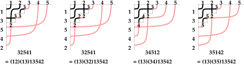
Figure 1. The four partial pipe dreams $D$ for $(\pi=13542$, $\lambda=2+1)$, with each one’s $\rho(D)$ written below it. Note that the tiles alone do not characterize the partial pipe dream; one must number the pipes. (When $\lambda$ is the full staircase every pipe connects to the North and West boundaries, determining its number.)

Theorem 5.1.

Fix $\pi\in S_{n}$ and $\lambda$ a partition with $\lambda_{i}\leq n-i,i\in[1,n]$. Then

$$C_{\pi}=\sum_{D}\frac{1}{\prod_{\ \hskip 0.1pt\smash{\raise 2.8pt\hbox{\co\hskip 4.15pt\hbox to0.0pt{\hbox to0.0pt{\char 5\relax\hss} \char 7\relax\hss} \lower 6.8pt\hbox to0.0pt{\vrule height=3.5pt\hss} \raise 3.6pt\hbox to0.0pt{\vrule height=3.5pt\hss}}\raise 2.8pt\hbox{\hbox to0.0pt{\hskip-7.15pt\vrule height=0.4pt,depth=0.0pt,width=3.5pt\hss}\hbox to0.0pt{\hskip 4.05pt\vrule height=0.4pt,depth=0.0pt,width=3.5pt\hss}}}\hskip 8.7pt\in D}(x_{row}-y_{col})}C_{\rho(D)}$$

where $D$ varies over the partial pipe dreams for $(\pi,\lambda)$. The dominant part of the Rothe diagram of each $\rho(D)$ contains $\lambda$, so each summand is polynomial.

Proof sketch..

Call two pipe dreams for $\pi$ $\lambda$-equivalent if they agree (in tiles and labels on pipes) inside $\lambda$. There is an obvious map from equivalence classes to partial pipe dreams, which we baldly assert to be bijective. If we take the pipe dreams in an equivalence class $D$ and replace all the     Π Υ           s in $\lambda$ with           s, we further assert that we get exactly the pipe dreams for $\rho(D)$. The result follows. ∎

If we take $\lambda$ to be the dominant part of $\pi$, then there is only one partial pipe dream $D$ for $(\pi,\lambda)$, where $\lambda$ is solid           s, and theorem 5.1 says $C_{\pi}=C_{\pi}$ (since $\rho(D)=\pi$). If we take $\lambda$ to have one more square at $(i,\pi(i))$, then the only freedom in $D$ is the choice $\ \hskip 0.1pt\smash{\raise 2.8pt\hbox{\co\hskip 4.15pt\hbox to0.0pt{\hbox to0.0pt{\char 5\relax\hss} \char 7\relax\hss} \lower 6.8pt\hbox to0.0pt{\vrule height=3.5pt\hss} \raise 3.6pt\hbox to0.0pt{\vrule height=3.5pt\hss}}\raise 2.8pt\hbox{\hbox to0.0pt{\hskip-7.15pt\vrule height=0.4pt,depth=0.0pt,width=3.5pt\hss}\hbox to0.0pt{\hskip 4.05pt\vrule height=0.4pt,depth=0.0pt,width=3.5pt\hss}}}\hskip 8.7pt_{j}$ of pipe label $j$ on that square, and theorem 5.1 becomes the generalized co-transition formula from §4. Finally, if we take $\lambda$ to be the full staircase $(n-1)+(n-2)+\ldots+1$, then every $D$ has $\rho(D)=w_{0}$, and theorem 5.1 recovers the definition of $C_{\pi}$ as a sum over pipe dreams.

6. Transition vs. co-transition

In [KnMi05] the Fulton determinants defining ${\overline{X}}_{\pi}$ were shown to be a Gröbner basis for antidiagonal term orders $<$, and the components of $init_{<}\ {\overline{X}}_{\pi}$ to be in obvious correspondence with $\pi$’s pipe dreams. There are four natural sources of antidiagonal term orders:

1. lexicographic, where the matrix entries are ordered from NE to SW (more precisely, by some linear extension of that partial order)

2. lexicographic, where the matrix entries are ordered from SW to NE

3. reverse lexicographic, where the matrix entries are ordered from NW to SE

4. reverse lexicographic, where the matrix entries are ordered from SE to NW.

Slicing ${\overline{X}}_{\pi}$ with the hyperplane $m_{i,\pi(i)}=0$ is a way of doing the first nontrivial step of the third kind of Gröbner degeneration, and hence, will a priori be compatible with the pipe dream combinatorics. (It is from there that the co-transition formula, and §3, were reverse-engineered. Stated more bluntly: after this insight, producing the rest of the paper was essentially an exercise.)

Define the co-dominant part outside $\pi$’s Rothe diagram as the set of matrix entries $(a,b)$ such that no Fulton determinant defining ${\overline{X}}_{\pi}$ involves $m_{ab}$. This is always connected to the SE corner of the square. Its complement is the boxes NW of some diagram box, or equivalently NW of some essential box. The $(i,j)$ in Lascoux’ transition formula was picked to be just outside the co-dominant part outside $\pi$’s Rothe diagram. See [KnYo04] for this view of the transition formula.

In unpublished work, Alex Yong and I gave a Gröbner-degeneration-based proof of Lascoux’ transition formula, based on one step of a lex order from SE to NW (so, not one of the orders above compatible with pipe dreams). For this reason, one might expect it to be very difficult to connect the pipe dream formula to the transition formula, requiring “Little bumping algorithms” and the like (see [BiHoYo17]), and essentially impossible if one wants to include the ${\underline{y}}$ variables. Indeed, it should be about as difficult as giving a bijective proof that two unimodular triangulations of a polytope should have the same number of simplices. (See [EsMé16] where polytopes arise from some matrix Schubert varieties, and this becomes more than an analogy.)

Recall the conormal variety $CX$ of a closed subvariety $X\subseteq V$ of a vector space:

$$CX:=\overline{\left\{(x,f)\in V\times V^{*}\ :\ x\in X\text{ a smooth point, }\vec{v}\perp T_{x}X\right\}}\quad\subseteq V\times V^{*}$$

Use the trace form to identify $M_{n}(\mathbb{C})^{*}$ with $M_{n}(\mathbb{C})$, and call two matrix Schubert varieties ${\overline{X}}_{\pi}$, ${\overline{X}}_{\rho}$ projective dual if $C{\overline{X}}_{\pi}\subseteq M_{n}(\mathbb{C})\times M_{n}(\mathbb{C})$ becomes $C{\overline{X}}_{\rho}$ upon switching the two $M_{n}(\mathbb{C})$ factors and rotating both matrices by $180^{\circ}$. (This is essentially the statement that the projective varieties $\mathbb{P}({\overline{X}}_{\pi}),\mathbb{P}({\overline{X}}_{\rho})$ are projective dual in the 19th-century sense; our reference is [Te05].) It is a fun exercise to determine $\rho$ from $\pi$; note that at least one of the two must be partial, not a permutation.

If ${\overline{X}}_{\pi}$ and ${\overline{X}}_{\rho}$ are projectively dual, then the dominant part of $\pi$’s diagram is the $180^{\circ}$ rotation of the co-dominant part outside $\rho$’s diagram – projective duality swaps zeroed-out coordinates with free coordinates.

Projective duality also exchanges lex term orders with revlex term orders. So finally, in this sense, the co-transition formula is related to the transition formula by projective duality. (The relation would be exact were to consider Gröbner degenerations of the conormal varieties, rather than of the matrix Schubert varieties themselves; since we only see the components in one $M_{n}(\mathbb{C})$ or the other the relation is more of an analogy.)

The reader may wonder, since the lex-from-NE term order was useful (this is effectively the approach in [Kn08]) and the revlex-from-NW term order was useful (in §4), why are the other two (at $180^{\circ}$ from these) left out? The $180^{\circ}$ symmetry is achieved if we refine the matrix Schubert variety stratification on $M_{n}(\mathbb{C})$ to the pullback of the positroid stratification on $Gr(n;\ \mathbb{C}^{2n})$ along the inclusion $graph:\,M_{n}(\mathbb{C})\hookrightarrow Gr(n;\ \mathbb{C}^{2n})$ regarding $M_{n}(\mathbb{C})$ as the big cell.

In [LaLeSh] was introduced an alternative family $\{C^{\prime}_{\pi}\}$ of “bumpless pipe dream” polynomials, and a proof that they match the double Schubert polynomials. The bijection from §3 deriving the co-transition formula for the pipe dream polynomials $\{C_{\pi}\}$ has a tightly analogous bijective proof of the transition formula for the $\{C^{\prime}_{\pi}\}$, in the recent preprint [We, §5].

7. Grothendieck polynomials, nonreduced pipe dreams,
and equivariant $K$-classes

All three families of polynomials $A,C,G$ have extensions to inhomogeneous Laurent polynomials $A^{\prime},C^{\prime},G^{\prime}$ in $\mathbb{Z}[\exp(\pm x_{1}),\exp(\pm x_{2}),\ldots,\exp(\pm y_{1}),\exp(\pm y_{2}),\ldots]$:

1. Double Grothendieck polynomials $A^{\prime}_{\pi}$. These satisfy recurrence relations based on isobaric Demazure operators.

2. Nonreduced pipe dream polynomials $C^{\prime}_{\pi}$. These allow pipes to cross twice. To read a permutation off of a (nonreduced) pipe dream, one follows the pipes, ignoring the second (and later) crossings of any two pipes.

3. Equivariant $K$-classes of matrix Schubert varieties $G^{\prime}_{\pi}$. The subvariety ${\overline{X}}_{\pi}\subseteq M_{n}(\mathbb{C})$ defines a class in $(T\times T)$-equivariant $K$-theory of $M_{n}(\mathbb{C})$.

Betraying our predilection towards geometry, we call each the “$K$-theoretic version” of the unprimed family, with the original being the “cohomological”.

Each $K$-theoretic family satisfies the same new base case

Lemma ($K$-theoretic base case).

For each family $P^{\prime}$ we have $P^{\prime}_{w_{0}^{n}}=\displaystyle\prod_{i,j\in[n],\ i+j\leq n}(1-\exp(y_{i}-x_{j}))$.

and the recurrence

Lemma (the $K$-theoretic co-transition formula).

Let $\pi,i,\{\rho\}$ be as in the cohomological co-transition formula. Let $S$ vary over the nonempty subsets of the set of such $\rho$. Then

$$(1-\exp(y_{\pi(i)}-x_{i}))\,P^{\prime}_{\pi}=\sum_{S}(-1)^{\#S-1}\,P^{\prime}_{l.u.b.(S)}$$

where $l.u.b.(S)$ is the (unique) least upper bound of $S$ in Bruhat order, automatically of length $\ell(\pi)+\#S$.

Intriguingly, this “boolean lattice inside Bruhat order” phenomenon shows up in the $K$-theoretic transition formula [La01] as well.

We won’t prove these two for $A^{\prime},C^{\prime},G^{\prime}$, but comment on the changes necessary from the cohomological proofs. (Of course, it is already known that $A^{\prime}=C^{\prime}=G^{\prime}$, see e.g. [KnMi05], so it suffices to prove these results for, say, just $G^{\prime}$.) The bijection in $C^{\prime}$, placing a            at $(i,\pi(i))$ where there was always a     Π Υ           , is the same. For the $G^{\prime}$ co-transition formula one needs to know that the intersection ${\overline{X}}_{\pi}\cap\left\{M:m_{ab}=0\ \forall(a,b)\text{ weakly NW of }(i,\pi(i))\right\}$ is reduced, and that each intersection $\cap_{S}{\overline{X}}_{\rho}={\overline{X}}_{l.u.b.(S)}$ is likewise reduced. The swiftest way to confirm this is to observe that there is a Frobenius splitting on the space of matrices (over each $\mathbb{F}_{p}$, rather than $\mathbb{C}$), with respect to which each ${\overline{X}}_{\pi}$ is compatibly split; as at the end of §6, one can infer this from the compatible splitting of the positroid varieties in the Grassmannian [KnLaSp13].

References

-
[BeCePi]
Nantel Bergeron, Cesar Ceballos, Vincent Pilaud,
Hopf dreams, preprint 2018.
https://arxiv.org/abs/1807.03044 -
[BeBi93]
Nantel Bergeron and Sara Billey, RC-graphs and Schubert
polynomials,
Experimental Math. 2 (1993), no. 4, 257–269. - [BiHoYo17] Sara Billey, Alexander Holroyd, Benjamin Young, A bijective proof of Macdonald’s reduced word formula, Algebraic Combinatorics 2(2) · February 2017.
-
[EsMé16]
Laura Escobar and Karola Mészáros,
Toric matrix Schubert varieties and their polytopes,
Proc. Amer. Math. Soc., 144(12):5081–5096, 2016. -
[Fu92]
William Fulton,
Flags, Schubert polynomials, degeneracy loci, and
determinantal formulas,
Duke Math. J.,65 (1992), 381–420. -
[Fu96]
William Fulton,
Young Tableaux,
With Applications to Representation Theory and Geometry,
Cambridge University Press, 1996. - [Fu99] William Fulton, Universal Schubert polynomials. Duke Math. J. 96 (1999), no. 3, 575–594.
- [Ka97] M. E. Kazarian, Characteristic classes of singularity theory, The Arnold-Gelfand mathematical seminars, Birkhäuser Boston, Boston, MA, 1997, pp. 325–340.
-
[Kn08]
Allen Knutson,
Schubert patches degenerate to subword complexes,
Transform. Groups 13 (2008), no. 3–4, 715–726. -
[KnLaSp13]
by same author, Thomas Lam, and David E Speyer,
Positroid varieties: juggling and geometry,
Compositio Mathematica, 149, (2013), no. 10, 1710–1752. -
[KnMi05]
by same authorand Ezra Miller,
Gröbner geometry of Schubert polynomials,
Annals of Mathematics, Volume 161 (2005), Issue 3, pp 1245–1318. - [KnYo04] by same authorand Alex Yong, A formula for K-theory truncation Schubert calculus, International Mathematics Research Notices, 70 (2004), 3741–3756.
- [LaLeSh] Thomas Lam, Seung Jin Lee, Mark Shimozono, Back stable Schubert calculus, preprint 2018.
-
[La01]
Alain Lascoux,
Transition on Grothendieck polynomials,
Physics and combinatorics, 2000 (Nagoya), 164–179, World Sci. Publishing, River Edge, NJ, 2001. - [La95] Alain Lascoux, Polynômes de Schubert: une approche historique, Discrete Mathematics, 139 (1): 303–317.
- [Te05] Jenia Tevelev, Projective duality and homogeneous spaces, Encyclopaedia of Mathematical Sciences, 133. Invariant Theory and Algebraic Transformation Groups, IV. Springer-Verlag, Berlin, 2005.
- [We] Anna Weigandt, Bumpless pipe dreams and alternating sign matrices, preprint 2020.