en-text

Parametric estimation for a parabolic linear SPDE model
based on sampled data

Abstract. We consider parametric estimation for a parabolic linear second order stochastic partial differential equation (SPDE) from high frequency data which are observed in time and space. By using thinned data obtained from the high frequency data, adaptive estimators of the coefficient parameters including the volatility parameter of a parabolic linear SPDE model are proposed. Moreover, we give some examples and simulation results of the adaptive estimators of the SPDE model based on the high frequency data.

Key words and phrases: adaptive estimation, diffusion process, high frequency data, stochastic partial differential equation, thinned data

1 Introduction

We consider a linear parabolic stochastic partial differential equation (SPDE) with one space dimension.

$$dX_{t}(y)=\left(\theta_{2}\frac{\partial^{2}X_{t}(y)}{\partial y^{2}}+\theta_{1}\frac{\partial X_{t}(y)}{\partial y}+\theta_{0}X_{t}(y)\right)dt+\sigma dB_{t}(y),\quad(t,y)\in[0,T]\times[0,1],\quad$$ (1)

$$X_{t}(0)=X_{t}(1)=0,\quad t\in[0,T],\qquad X_{0}(y)=\xi=0,\quad y\in[0,1],$$

where $T>0$, $B_{t}$ is defined as a cylindrical Brownian motion in the Sobolev space on $[0,1]$, the initial condition $\xi=0$, an unknown parameter $\theta=(\theta_{0},\theta_{1},\theta_{2},\sigma)$ and $\theta_{0},\theta_{1}\in\mathbb{R},\theta_{2},\sigma>0$, and the parameter space $\Theta$ is a compact convex subset of $\mathbb{R}^{2}\times[0,\infty]^{2}$. Moreover, the true value of parameter $\theta^{*}=(\theta_{0}^{*},\theta_{1}^{*},\theta_{2}^{*},\sigma^{*})$ and we assume that $\theta^{*}\in\mbox{Int}(\Theta)$. The data are discrete observations ${\bf X}_{N,M}=\left\{X_{t_{i:N}}(y_{j:M})\right\}_{i=1,...,N,j=1,...,M}$, $t_{i:N}=i\frac{T}{N}$, ${y_{j:M}=\frac{j}{M}}$. For the characteristics of the parameters $\theta_{0}$, $\theta_{1}$, $\theta_{2}$ and $\sigma$ of the SPDE (1), see the Appendix below.

Statistical inference for SPDE models based on sampled data has been developed by many researchers, see for example, Markussen (2003), Cont (2005), Cialenco and Glatt-Holtz (2011), Cialenco and Huang (2017), Bibinger and Trabs (2017), Cialenco et. al. (2018, 2019), Cialenco (2018), Chong (2019) and references therein. Recently, Bibinger and Trabs (2017) studied the parabolic linear second order SPDE model based on high frequency data observed on a fixed region and proved the asymptotic properties of minimum contrast estimators $\check{\sigma}_{0}^{2}$ and $\check{\eta}$ for both the normalized volatility parameter $\sigma_{0}^{2}=\frac{\sigma^{2}}{\sqrt{\theta_{2}}}$ and the curvature parameter $\eta=\frac{\theta_{1}}{\theta_{2}}$.

In this paper, we propose adaptive maximum likelihood (ML) type estimator of the coefficient parameter $\theta=(\theta_{0},\theta_{1},\theta_{2},\sigma)$ of the parabolic linear second order SPDE model (1). For $k\in\mathbb{N}$, the coordinate process $x_{k}(t)$ of the SPDE model (1) is that

$$x_{k}(t) = \int^{1}_{0}X_{t}(y)\sqrt{2}\sin(\pi ky)\exp\left(\frac{\eta y}{2}\right)dy,$$ (2)

which satisfies that

$$dx_{k}(t)=-\lambda_{k}x_{k}(t)dt+\sigma dw_{k}(t),\quad x_{k}(0)=0,$$

where

$$\lambda_{k} = -\theta_{0}+\frac{\theta_{1}^{2}}{4\theta_{2}}+\pi^{2}k^{2}\theta_{2}.$$

Note that the coordinate process (2) is the Ornstein-Uhlenbeck process. Using the minimum contrast estimator $\check{\eta}$ proposed by Bibinger and Trabs (2017), we obtain the approximate coordinate process

$$\check{x}_{k}(t)=\frac{1}{M}\sum^{M}_{j=1}X_{t}(y_{j:M})\sqrt{2}\sin(\pi ky_{j:M})\exp\left(\frac{\check{\eta}y_{j:M}}{2}\right)$$

and the adaptive estimator is constructed by using the property that the coordinate process (2) is a diffusion process. It is also shown that the adaptive ML type estimators have asymptotic normality under some regularity conditions. Furthermore, in order to verify asymptotic performance of the adaptive ML type estimators of the coefficient parameters of the parabolic linear second order SPDE model based on high-frequency data, some examples and simulation results of the adaptive ML type estimators are given. For details of statistical inference for diffusion type processes and stochastic differential equations, see Prakasa Rao (1983,1988), Kutoyants (1994, 2004), Florens-Zmirou (1989), Yoshida (1992, 2011), Bibby and Sørensen (1995), Kessler (1995, 1997), Uchida (2010), Uchida and Yoshida (2012, 2014), De Gregorio and Iacus (2013), Kamatani and Uchida (2015), Nakakita and Uchida (2019) for ergodic diffusion processes, and Shimizu and Yoshida (2006), Shimizu (2006), Ogihara and Yoshida (2011), Masuda (2013a, 2013b) for jump diffusion processes and Lévy type processes, and Dohnal (1987), Genon-Catalot and Jacod (1993, 1994), Uchida and Yoshida (2013), Ogihara and Yoshida (2014), Ogihara (2018), Kaino and Uchida (2018) for non-ergodic diffusion processes. For adaptive ML type estimators and thinned data for diffusion type processes, see for example, Uchida and Yoshida (2012) and Kaino and Uchida (2018).

This paper is organized as follows. In Section 2, we consider the adaptive estimator of the SPDE model based on the sampled data in the fixed region $[0,1]\times[0,1]$. The adaptive estimator is constructed by using the minimum contrast estimators of $\sigma_{0}^{2}$ and $\eta$ proposed by Bibinger and Trabs (2017). It is shown that the adaptive estimator has asymptotic normality. In Section 3, we deal with the SPDE model based on sampled data which are observed in the region $[0,T]\times[0,1]$ when $T$ is large. The quasi log likelihood function is obtained by using the approximate coordinate process and we prove that the adaptive ML type estimator of $\theta=(\theta_{0},\theta_{1},\theta_{2},\sigma)$ has asymptotic normality. In Section 4, concrete examples are given and the asymptotic behavior of the estimators proposed in Sections 2 and 3 is verified by simulations. Section 5 is devoted to the proofs of the results presented in Sections 2 and 3. The Appendix contains the sample paths with different values of the parameters to understand the characteristics of the parameters $\theta_{0}$, $\theta_{1}$, $\theta_{2}$ and $\sigma$ of the SPDE (1).

2 The case that T is fixed

In this section, we treat the linear parabolic SPDE (1) with $T=1$, which is defined as

$$dX_{t}(y)=\left(\theta_{2}\frac{\partial^{2}X_{t}(y)}{\partial y^{2}}+\theta_{1}\frac{\partial X_{t}(y)}{\partial y}+\theta_{0}X_{t}(y)\right)dt+\sigma dB_{t}(y),\quad(t,y)\in[0,1]\times[0,1],\quad$$ (3)

$$X_{t}(0)=X_{t}(1)=0,\quad t\in[0,1],\qquad X_{0}(y)=\xi=0,\quad y\in[0,1].$$

The data are discrete observations ${{\bf\bar{X}}_{N,\bar{M}}}=\left\{X_{t_{i:N}}({\bar{y}_{j:M}})\right\}_{i=1,\ldots,N,j=1,\ldots,{\bar{M}}}$ with $t_{i:N}=\frac{i}{N}$, $\bar{y}_{j:M}=\delta+\frac{j-1}{M}$ and $\bar{M}=[(1-2\delta)M]$ for $\delta\in(0,1/2)$. Note that $\delta\leq\bar{y}_{j:M}\leq 1-\delta$ for $j=1,\ldots,\bar{M}$, and that ${\bf\bar{X}}_{N,\bar{M}}$ is generated by the full data ${\bf X}_{N,M}=\left\{X_{t_{i:N}}(y_{j:M})\right\}_{i=1,...,N,j=1,...,M}$ with $t_{i:N}=\frac{i}{N}$ and $y_{j:M}=\frac{j}{M}$.

Setting that the differential operator

$$A_{\theta}:=\theta_{0}+\theta_{1}\frac{\partial}{\partial y}+\theta_{2}\frac{\partial^{2}}{\partial y^{2}},$$

one has that for $k\in\mathbb{N}$,

$$A_{\theta}e_{k}=-\lambda_{k}e_{k},$$

where the eigenfunctions $e_{k}$ of $A_{\theta}$ and the corresponding eigenvalues $-\lambda_{k}$ are given by

$$e_{k}(y) = \sqrt{2}\sin(\pi ky)\exp\left(-\frac{\theta_{1}}{2\theta_{2}}y\right),\;\;\;y\in[0,1],$$

$$\lambda_{k} = -\theta_{0}+\frac{\theta_{1}^{2}}{4\theta_{2}}+\pi^{2}k^{2}\theta_{2}.$$

Let $H_{\theta}:=\{f:[0,1]\to\mathbb{R}:\|f\|_{\theta}<\infty,f(0)=f(1)=0\}$ with $\langle f,g\rangle_{\theta}:=\int^{1}_{0}e^{y\theta_{1}/\theta_{2}}f(y)g(y)dy$ and $\|f\|_{\theta}:=\sqrt{\langle f,f\rangle_{\theta}}$. The initial condition $\xi(y)=0$ and $\xi\in H_{\theta}$.

2.1 Estimation of $\sigma_{0}^{2}$ and $\eta$

Set $\sigma_{0}^{2}=\frac{\sigma^{2}}{\sqrt{\theta_{2}}}$, $\eta=\frac{\theta_{1}}{\theta_{2}}$. Let $m\leq{\bar{M}}$ and $\tilde{y}_{j:m}={\delta+}\left[\frac{{\bar{M}}}{m}\right]{\frac{j-1}{M}}$ for $j=1,...,m$. Assume that $m\leq N^{\rho}$ for $\rho\in(0,1/2)$. Set

$$Z_{j:m}=\frac{1}{N\sqrt{{t}_{1:N}}}\sum_{i=1}^{N}(X_{\tilde{t}_{i:N}}(\tilde{y}_{j:m})-X_{\tilde{t}_{i-1:N}}(\tilde{y}_{j:m}))^{2}.$$

The contrast function is defined as

$$U_{N,m}(\sigma_{0}^{2},\eta)=\frac{1}{m}\sum^{m}_{j=1}\left(Z_{j:m}-\frac{1}{\sqrt{\pi}}\sigma_{0}^{2}\exp(-\eta\tilde{y}_{j:m})\right)^{2}.$$

The minimum contrast estimator of $\sigma_{0}^{2}$ and $\eta$ are given by

$$(\check{\sigma}_{0}^{2},\check{\eta})=\mathop{\rm arg~{}inf}\limits_{\sigma_{0}^{2},\eta}U_{N,m}(\sigma_{0}^{2},\eta).$$

Let

$$U(\zeta^{*}) = \begin{pmatrix}\int^{1-\delta}_{\delta}e^{-4\eta^{*}y}dy&-(\sigma^{*}_{0})^{2}\int^{1-\delta}_{\delta}ye^{-4\eta^{*}y}dy\\ -(\sigma_{0}^{*})^{2}\int^{1-\delta}_{\delta}ye^{-4\eta^{*}y}dy&(\sigma^{*}_{0})^{4}\int^{1-\delta}_{\delta}y^{2}e^{-4\eta^{*}y}dy\end{pmatrix},$$

$$V(\zeta^{*}) = \begin{pmatrix}\int^{1-\delta}_{\delta}e^{-2\eta^{*}y}dy&-(\sigma^{*}_{0})^{2}\int^{1-\delta}_{\delta}ye^{-2\eta^{2}y}dy\\ -(\sigma^{*}_{0})^{2}\int^{1-\delta}_{\delta}ye^{-2\eta^{*}y}dy&(\sigma^{*}_{0})^{4}\int^{1-\delta}_{\delta}y^{2}e^{-2\eta^{*}y}dy\end{pmatrix},$$

$$\Gamma = \frac{1}{\pi}\sum^{\infty}_{r=0}I(r)^{2}+\frac{2}{\pi}\ \mbox{with}\ I(r)=2\sqrt{r+1}-\sqrt{r+2}-\sqrt{r}.$$

Theorem 1 (Bibinger and Trabs(2017))

Let $\zeta^{*}=((\sigma_{0}^{*})^{2},\eta^{*})\in\Xi$ for a compact subset $\Xi\subseteq(0,\infty)\times[0,\infty)$. Assume that $m\to\infty$ and $m=\mathcal{O}(N^{\rho})$ for some $\rho\in(0,1/2)$. Then, as $N\to\infty$,

$$\sqrt{mN}(\check{\sigma}_{0}^{2}-(\sigma_{0}^{*})^{2},\check{\eta}-\eta^{*})\stackrel{{\scriptstyle d}}{{\longrightarrow}}N(0,(\sigma_{0}^{*})^{4}\Gamma\pi V(\zeta^{*})^{-1}U(\zeta^{*})V(\zeta^{*})^{-1}).$$

2.2 Estimation of $\theta_{1},\theta_{2}$ and $\sigma^{2}$

Next we consider the estimation of $\sigma,\theta_{1},\theta_{2}$ using $\check{\sigma}_{0}^{2},\check{\eta}$. Let $k\in\mathbb{N}$. The coordinate process is that

$$x_{k}(t) = \langle X_{t},e_{k}\rangle_{\theta}=\int^{1}_{0}\exp\left(\frac{\theta_{1}}{\theta_{2}}y\right)X_{t}(y)e_{k}(y)dy$$

$$= \int^{1}_{0}X_{t}(y)\sqrt{2}\sin(\pi ky)\exp\left(\frac{\eta y}{2}\right)dy.$$

Note that

$$dx_{k}(t)=-\lambda_{k}x_{k}(t)dt+\sigma dw_{k}(t),\quad x_{k}(0)=0,$$

which means that $x_{k}(t)$ is the Ornstein-Uhlenbeck process. Furthermore, the random field $X_{t}(y)$ is that

$$X_{t}(y)=\sum_{k=1}^{\infty}x_{k}(t)e_{k}(y).$$

Let $N_{2}\leq N$ and ${s}_{i:N_{2}}=\left[\frac{N}{N_{2}}\right]t_{i:N}=i\left[\frac{N}{N_{2}}\right]\frac{1}{N}$ for $i=1,...,N_{2}$． As an approximation of $x_{k}(t)$, we consider

$$\check{x}_{k}({s}_{i:N_{2}})=\frac{1}{M}\sum^{M}_{j=1}X_{{s}_{i:N_{2}}}(y_{j:M})\sqrt{2}\sin(\pi ky_{j:M})\exp\left(\frac{\check{\eta}y_{j:M}}{2}\right),\quad i=1,...,N_{2}.$$

By using the thinned data based on the approximate coordinate process $\left\{\check{x}_{k}(s_{i:N_{2}})\right\}_{i=1,\ldots,N_{2}}$, the estimator of $\sigma^{2}$ is defined as

$$\check{\sigma}_{k}^{2}=\sum^{N_{2}}_{i=1}(\check{x}_{k}({s}_{i:N_{2}})-\check{x}_{k}({s}_{i-1:N_{2}}))^{2}.$$

Set $k=1$ and $\check{\sigma}^{2}=\check{\sigma}_{1}^{2}$． The estimators of $\theta_{1}$ and $\theta_{2}$ are defined as

$$\check{\theta}_{2}=\left(\frac{\check{\sigma}^{2}}{\check{\sigma}_{0}^{2}}\right)^{2},\quad\check{\theta}_{1}=\check{\eta}\check{\theta_{2}}.$$

Theorem 2

Assume the same conditions as Theorem 1. Moreover, assume that $\frac{N_{2}^{3/2}}{mN}\rightarrow 0$ and $\frac{N_{2}^{3/2}}{M^{1-\rho_{1}}}\rightarrow 0$ for $\rho_{1}\in(0,1)$. Then, as $N_{2}\rightarrow\infty$,

$$\begin{pmatrix}\sqrt{N_{2}}(\check{\sigma}^{2}-(\sigma^{*})^{2})\\ \sqrt{N_{2}}(\check{\theta}_{2}-\theta_{2}^{*})\\ \sqrt{N_{2}}(\check{\theta}_{1}-\theta_{1}^{*})\end{pmatrix}\stackrel{{\scriptstyle d}}{{\longrightarrow}}N\left(\begin{pmatrix}0\\ 0\\ 0\end{pmatrix},\begin{pmatrix}2(\sigma^{*})^{4}&4\theta_{2}^{*}(\sigma^{*})^{2}&4\theta_{1}^{*}(\sigma^{*})^{2}\\ 4\theta_{2}^{*}(\sigma^{*})^{2}&8(\theta_{2}^{*})^{2}&8\theta_{1}^{*}\theta_{2}^{*}\\ 4\theta_{1}^{*}(\sigma^{*})^{2}&8\theta_{1}^{*}\theta_{2}^{*}&8(\theta_{1}^{*})^{2}\end{pmatrix}\right)$$

3 The case that $T$ is large

In this section, we deal with the linear parabolic SPDE (1) when $T$ is large, which is defined as

$$dX_{t}(y)=\left(\theta_{2}\frac{\partial^{2}X_{t}(y)}{\partial y^{2}}+\theta_{1}\frac{\partial X_{t}(y)}{\partial y}+\theta_{0}X_{t}(y)\right)dt+\sigma dB_{t}(y),\quad(t,y)\in[0,T]\times[0,1],\quad$$ (4)

$$X_{t}(0)=X_{t}(1)=0,\quad t\in[0,T],\qquad X_{0}(y)=\xi=0,\quad y\in[0,1].$$

The data are discrete observations ${{\bf\check{X}}_{N,\bar{M}}}=\left\{X_{t_{i:N}}({\bar{y}_{j:M}})\right\}_{i=1,...,N,j=1,...,{\bar{M}}}$ with $t_{i:N}=ih_{N:T}$, $h_{N:T}=\frac{T}{N}$, $\bar{y}_{j:M}=\delta+\frac{j-1}{M}$ and $\bar{M}=[(1-2\delta)M]$ for $\delta\in(0,1/2)$. Note that $\delta\leq\bar{y}_{j:M}\leq 1-\delta$ for $j=1,\ldots,\bar{M}$, and that ${\bf\check{X}}_{N,\bar{M}}$ is generated by the full data ${\bf X}_{N,M}=\left\{X_{t_{i:N}}(y_{j:M})\right\}_{i=1,...,N,j=1,...,M}$ with $t_{i:N}=ih_{N:T}$ and $y_{j:M}=\frac{j}{M}$.

3.1 Estimation of $\sigma_{0}^{2},\eta$

Let $\bar{m}\leq{\bar{M}}$ and $\tilde{y}_{j:\bar{m}}={\delta+}\left[\frac{{\bar{M}}}{\bar{m}}\right]{\frac{j-1}{M}}$ for $j=1,...,\bar{m}$. Set

$$\bar{{\cal Z}}_{j:\bar{m}}=\frac{1}{N\sqrt{h_{N:T}}}\sum_{i=1}^{N}(X_{t_{i:N:T}}(\tilde{y}_{j:\bar{m}})-X_{t_{i-1:N:T}}(\tilde{y}_{j:\bar{m}}))^{2}.$$

The contrast function is defined as

$$\bar{{\cal U}}_{N,\bar{m}}(\sigma_{0}^{2},\eta)=\frac{1}{\bar{m}}\sum^{\bar{m}}_{j=1}\left(\bar{{\cal Z}}_{j:\bar{m}}-\frac{1}{\sqrt{\pi}}\sigma_{0}^{2}\exp(-\eta\tilde{y}_{j:\bar{m}})\right)^{2}.$$

The minimum contrast estimator of $\sigma_{0}^{2}$ and $\eta$ are given by

$$(\hat{\sigma}_{0}^{2},\hat{\eta})=\mathop{\rm arg~{}inf}\limits_{\sigma_{0}^{2},\eta}\bar{{\cal U}}_{N,\bar{m}}(\sigma_{0}^{2},\eta).$$

Theorem 3

Assume that $Nh_{N:T}^{2}\rightarrow 0$, $\bar{m}\rightarrow\infty$ and $\bar{m}=O(h_{N:T}^{-\rho})$ for $\rho\in(0,1/2)$. Then, as $N\to\infty$,

$$\sqrt{\bar{m}N}(\hat{\sigma}_{0}^{2}-(\sigma_{0}^{*})^{2},{\hat{\eta}}-\eta^{*})\stackrel{{\scriptstyle d}}{{\longrightarrow}}N(0,(\sigma_{0}^{*})^{4}\Gamma\pi V(\zeta^{*})^{-1}U(\zeta^{*})V(\zeta^{*})^{-1}).$$

Next we consider the case that $\bar{m}$ is fixed. Let

$$U_{\bar{m}}(\zeta^{*}) = \begin{pmatrix}\sum_{j=1}^{\bar{m}}e^{-4\eta^{*}y_{j:\bar{m}}}&-(\sigma^{*}_{0})^{2}\sum_{j=1}^{\bar{m}}y_{j:\bar{m}}e^{-4\eta^{*}y_{j:\bar{m}}}\\ -(\sigma^{*}_{0})^{2}\sum_{j=1}^{\bar{m}}y_{j:\bar{m}}e^{-4\eta^{*}y_{j:\bar{m}}}&(\sigma^{*}_{0})^{4}\sum_{j=1}^{\bar{m}}y_{j:\bar{m}}e^{-4\eta^{*}y_{j:\bar{m}}^{2}}\end{pmatrix},$$

$$V_{m}(\zeta^{*}) = \begin{pmatrix}\sum_{j=1}^{\bar{m}}e^{-2\eta^{*}y_{j:\bar{m}}}&-(\sigma^{*}_{0})^{2}\sum_{j=1}^{\bar{m}}y_{j:\bar{m}}e^{-2\eta^{*}y_{j:\bar{m}}}\\ -(\sigma^{*}_{0})^{2}\sum_{j=1}^{\bar{m}}y_{j:\bar{m}}e^{-2\eta^{*}y_{j:\bar{m}}}&(\sigma^{*}_{0})^{4}\sum_{j=1}^{\bar{m}}y_{j:\bar{m}}^{2}e^{-2\eta^{*}y_{j:\bar{m}}^{2}}\end{pmatrix}.$$

Corollary 1

Let $\bar{m}\geq 2$. Assume that $Nh_{N:T}^{2}\rightarrow 0$. Then, as $N\to\infty$,

$$\sqrt{N}(\hat{\sigma}_{0}^{2}-(\sigma_{0}^{*})^{2},{\hat{\eta}}-\eta^{*})\stackrel{{\scriptstyle d}}{{\longrightarrow}}N(0,(\sigma_{0}^{*})^{4}\Gamma\pi V_{\bar{m}}(\zeta^{*})^{-1}U_{\bar{m}}(\zeta^{*})V_{\bar{m}}(\zeta^{*})^{-1}).$$

3.2 Estimation of four parameters

Next we consider the estimation of $\sigma,\theta_{1},\theta_{2},$ and $\theta_{0}$ using $\hat{\sigma}_{0}^{2}$ and $\hat{\eta}$. Let $k\in\mathbb{N}$. As an approximation of $x_{k}(t)$, we consider

$$\bar{x}_{k}(t_{i:N:T})=\frac{1}{M}\sum^{M}_{j=1}X_{t_{i:N:T}}(y_{j:M})\sqrt{2}\sin(\pi ky_{j:M})\exp\left(\frac{\hat{\eta}y_{j:M}}{2}\right),\quad i=1,...,N.$$

Let $\bar{N}_{2}\leq N$, $\delta_{\bar{N}_{2}:T}=\left[\frac{N}{\bar{N}_{2}}\right]h_{N:T}=\left[\frac{N}{\bar{N}_{2}}\right]\frac{T}{N}$ and $s_{i:\bar{N}_{2}:T}=i\delta_{\bar{N}_{2}:T}$ for $i=1,...,\bar{N}_{2}$. The quasi log-likelihood function with the thinned data based on the approximate coordinate process ${\bf\bar{x}}_{k}=\{\bar{x}_{k}(s_{i:\bar{N}_{2}:T})\}_{i=1,\ldots,\bar{N}_{2}}$ is defined as

$$l_{\bar{N}_{2}}(\lambda_{k},\sigma^{2}\ |\ {\bf\bar{x}}_{k}) = -\sum^{\bar{N}_{2}}_{i=1}\left\{\frac{1}{2}\log\left(\frac{\sigma^{2}(1-\exp(-2\lambda_{k}\delta_{\bar{N}_{2}:T}))}{2\lambda_{k}}\right)\right.$$

$$\left.+\frac{(\bar{x}_{k}(s_{i:\bar{N}_{2}:T})-\exp(-\lambda_{k}\delta_{\bar{N}_{2}:T})\bar{x}_{k}(s_{i-1:\bar{N}_{2}:T}))^{2}}{\frac{2\sigma^{2}(1-\exp(-2\lambda_{k}\delta_{\bar{N}_{2}:T}))}{2\lambda_{k}}}\right\}.$$

The quasi maximum likelihood estimator of $(\lambda_{k},\sigma^{2})$ is defined as

$$(\hat{\lambda}_{k},\hat{\sigma}^{2}_{k})=\mathop{\rm arg~{}sup}\limits_{\lambda,\sigma^{2}}l_{\bar{N}_{2}}(\lambda,\sigma^{2}\ |\ {\bf\bar{x}}_{k}).$$

Set $k=1$, $\hat{\lambda}=\hat{\lambda}_{1},\hat{\sigma}^{2}=\hat{\sigma}^{2}_{1}$. Note that $\lambda_{1}^{*}=-\theta_{0}^{*}+\frac{(\theta_{1}^{*})^{2}}{4\theta_{2}^{*}}+\pi^{2}\theta_{2}^{*}$. The estimators of $\theta_{1}$, $\theta_{2}$ are defined as

$$\hat{\theta}_{2}=\left(\frac{\hat{\sigma}^{2}}{\hat{\sigma}_{0}^{2}}\right)^{2},\quad\hat{\theta}_{1}=\hat{\eta}\hat{\theta_{2}}.$$

The estimator of $\theta_{0}$ is defined as

$$\hat{\theta}_{0}=-\hat{\lambda}+\frac{\hat{\theta}_{1}^{2}}{4\hat{\theta}_{2}}+\pi^{2}\hat{\theta}_{2}.$$

Theorem 4

Assume the same conditions as Theorem 3. Moreover, assume that $\frac{\bar{N}_{2}^{\frac{5}{2}}}{T^{\frac{3}{2}}N\bar{m}}\to 0$ and $\frac{\bar{N}_{2}^{3}}{T^{2}M^{1-\rho_{1}}}\to 0$ for $\rho_{1}\in(0,1)$. Then, as $\bar{N}_{2}\to\infty$,

$$\begin{pmatrix}\sqrt{N_{2}}((\hat{\sigma})^{2}-(\sigma^{*})^{2})\\ \sqrt{N_{2}}(\hat{\theta}_{2}-\theta_{2}^{*})\\ \sqrt{N_{2}}(\hat{\theta}_{1}-\theta_{1}^{*})\\ \sqrt{T}(\hat{\theta}_{0}-\theta_{0}^{*})\end{pmatrix}\stackrel{{\scriptstyle d}}{{\longrightarrow}}N\left(\begin{pmatrix}0\\ 0\\ 0\\ 0\end{pmatrix},\begin{pmatrix}2(\sigma^{*})^{4}&4\theta_{2}^{*}(\sigma^{*})^{2}&4\theta_{1}^{*}(\sigma^{*})^{2}&0\\ 4\theta_{2}^{*}(\sigma^{*})^{2}&8(\theta_{2}^{*})^{2}&8\theta_{1}^{*}\theta_{2}^{*}&0\\ 4\theta_{1}^{*}(\sigma^{*})^{2}&8\theta_{1}^{*}\theta_{2}^{*}&8(\theta_{1}^{*})^{2}&0\\ 0&0&0&2\lambda^{*}_{1}\end{pmatrix}\right).$$

Corollary 2

Let $\bar{m}\geq 2$. Assume the same conditions as Corollary 1. Moreover, assume that $\frac{\bar{N}_{2}^{\frac{5}{2}}}{T^{\frac{3}{2}}N}\to 0$ and $\frac{\bar{N}_{2}^{3}}{T^{2}M^{1-\rho_{1}}}\to 0$ for $\rho_{1}\in(0,1)$. Then, as $\bar{N}_{2}\to\infty$,

$$\begin{pmatrix}\sqrt{N_{2}}((\hat{\sigma})^{2}-(\sigma^{*})^{2})\\ \sqrt{N_{2}}(\hat{\theta}_{2}-\theta_{2}^{*})\\ \sqrt{N_{2}}(\hat{\theta}_{1}-\theta_{1}^{*})\\ \sqrt{T}(\hat{\theta}_{0}-\theta_{0}^{*})\end{pmatrix}\stackrel{{\scriptstyle d}}{{\longrightarrow}}N\left(\begin{pmatrix}0\\ 0\\ 0\\ 0\end{pmatrix},\begin{pmatrix}2(\sigma^{*})^{4}&4\theta_{2}^{*}(\sigma^{*})^{2}&4\theta_{1}^{*}(\sigma^{*})^{2}&0\\ 4\theta_{2}^{*}(\sigma^{*})^{2}&8(\theta_{2}^{*})^{2}&8\theta_{1}^{*}\theta_{2}^{*}&0\\ 4\theta_{1}^{*}(\sigma^{*})^{2}&8\theta_{1}^{*}\theta_{2}^{*}&8(\theta_{1}^{*})^{2}&0\\ 0&0&0&2\lambda^{*}_{1}\end{pmatrix}\right).$$

4 Examples and simulation results

In the same way as Bibinger and Trabs (2017), the numerical solution of the SPDE (1) is generated by

$$\tilde{X}_{t_{i:N}}(y_{j:M})=\sum^{K}_{k=1}x_{k}(t_{i:N})e_{k}(y_{j:M}),\quad i=1,...,N,j=1,...,M,$$ (5)

where

$$x_{k}(t_{i:N})=\exp\left(-\lambda_{k}\frac{T}{N}\right)x_{k}(t_{i-1:N})+\sqrt{\frac{\sigma^{2}(1-\exp(-2\lambda_{k}\frac{T}{N}))}{2\lambda_{k}}}N(0,1),\quad i=1,...,N.$$

When the tuning parameter $K$ is not large enough, the approximation (5) does not work well and the estimators in Theorem 1 and Theorem 3 have considerable biases. Therefore, the tuning parameter $K$ needs $10^{5}$ or more.

4.1 The case that $T$ is fixed

In this subsection, we consider the linear parabolic SPDE (3) where the true value $(\theta_{0},\theta_{1},\theta_{2},\sigma)=(0,0.5,0.1,1)$. We set that $N=10^{4}$, $M=10^{4}$, $K=10^{5}$, $T=1$. When $N=M=10^{4}$, the size of data ${\bf X}_{N,M}$ is about 1 GB. We used R language to compute the estimators of Theorems 1 and 2. The personal computer with Intel Gold 6128 (3.40GHz) was used for this simulation. It takes about 4 hours to generate one sample path of the SPDE (3) with $N=10^{4}$, $M=10^{4}$, $K=10^{5}$, $T=1$.

Figure 1 is a sample path of $X_{t}(y)$ for $(t,y)\in[0,1]\times[0,1]$ when $(\theta_{0},\theta_{1},\theta_{2},\sigma)=(0,0.5,0.1,1)$.

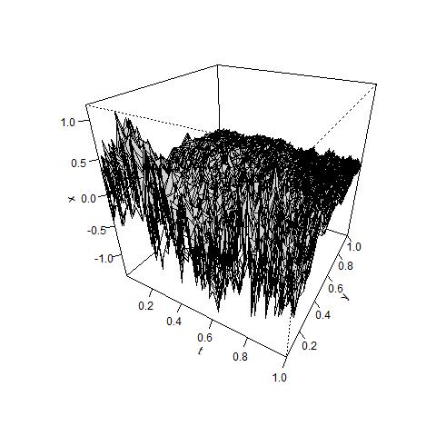
Figure 1: Sample path with $\theta=(0,0.5,0.1,1)$

Figures 2-4 are the simulation results of $\check{\sigma}^{2}$, $\check{\theta}_{2}$ and $\check{\theta}_{1}$ in Theorem 2 with $(N,m,N_{2})=(10^{4},99,333)$. Note that $\frac{N_{2}^{3/2}}{mN}\approx 0.006$, $\frac{N_{2}^{3/2}}{M^{0.99}}\approx 0.66$ and the number of iteration is $1000$. The left side of Figure 2 is the plot of the empirical distribution function of $\sqrt{N_{2}}(\check{\sigma}^{2}-(\sigma^{*})^{2})$ (black line) and the distribution function of $N(0,2(\sigma^{*})^{4})$ (red line). The center of Figure 2 is the Q-Q plot of $\sqrt{N_{2}}(\check{\sigma}^{2}-(\sigma^{*})^{2})$ and $N(0,2(\sigma^{*})^{4})$. The right side of Figure 2 is the plot of the histogram of $\sqrt{N_{2}}(\check{\sigma}^{2}-(\sigma^{*})^{2})$ and the density function of $N(0,2(\sigma^{*})^{4})$ (red line). Figures 3 and 4 are the plots of the empirical distribution functions, the Q-Q plots and the histograms of $\sqrt{N_{2}}(\check{\theta}_{2}-\theta_{2}^{*})$ and $\sqrt{N_{2}}(\check{\theta}_{1}-\theta_{1}^{*})$, respectively. From Figures 2-4, we can see that the distributions of the estimators in Theorem 2 almost correspond with the asymptotic distribution and these estimates have good performance.

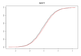
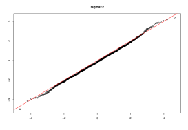
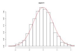
Figure 2: Simulation results of $\check{\sigma}^{2}$

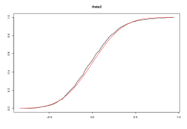
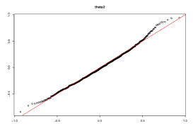
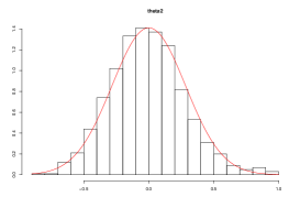
Figure 3: Simulation results of $\check{\theta}_{2}$

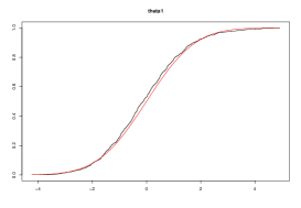
Figure 4: Simulation results of $\check{\theta}_{1}$

4.2 The case that $T$ is large

In this subsection, we deal with the linear parabolic SPDE (4) where the true value $(\theta_{0},\theta_{1},\theta_{2},\sigma)=(0,0.2,0.2,1)$ and we set $N=10^{5}$, $M=10^{5}$, $K=10^{5}$, $T=100$. When $N=M=10^{5}$, ${\bf X}_{N,M}$ is about 80 GB, which is too large for R to handle. We use the Python Programming Language to compute the estimators of Theorems 3 and 4. It takes about 30 hours to generate one sample path of the SPDE (4) with $N=10^{5}$, $M=10^{5}$, $K=10^{5}$, $T=100$.

Figure 5 is a sample path of $X_{t}(y)$ for $(t,y)\in[0,100]\times[0,1]$ when $(\theta_{0},\theta_{1},\theta_{2},\sigma)=(0,0.2,0.2,1)$.

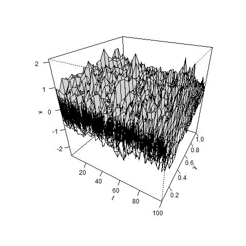
Figure 5: Sample path with $\theta=(0,0.2,0.2,1)$

We set $\bar{m}=24$ and the number of iteration is $300$. Figure 6 is the plots of the empirical distribution functions of $\sqrt{\bar{m}N}(\hat{\sigma}_{0}^{2}-(\sigma_{0}^{*})^{2})$ and $\sqrt{\bar{m}N}(\bar{\eta}-\eta^{*})$ in Theorem 3, respectively. The red lines in Figure 6 are the plots of the distribution functions of the corresponding asymptotic distributions. From Figure 6, we can see that the empirical distributions of the estimators in Theorem 3 almost fit the asymptotic distribution and these estimates have good behavior. This result indicates that the estimators work well when $N=10^{5}$ and $\bar{m}=24$.

Figure 6: Simulation results of $\hat{\sigma}_{0}^{2}$ (left) and $\hat{\eta}$ (right) in Theorem 3

Figures 7-10 are the simulation results of $\hat{\sigma}^{2}$, $\hat{\theta}_{2}$, $\hat{\theta}_{1}$ and $\hat{\theta}_{0}$ in Theorem 4 with $(N,{\bar{m}},T,{\bar{N}_{2}})=(10^{5},24,100,800)$. Note that $\frac{\bar{N}_{2}^{\frac{5}{2}}}{T^{\frac{3}{2}}\bar{m}N}=0.0075$ and $\frac{\bar{N}_{2}^{3}}{T^{2}M^{1-0.01}}=0.57$. From Figures 7-10, we can see that these estimates have good performance. When $T$ is large, we can estimate all parameters, $\theta_{0}$, $\theta_{1}$, $\theta_{2}$ and $\sigma$ of the SPDE (4).

Figure 7: Simulation results of $\hat{\sigma}^{2}$

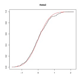
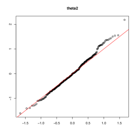
Figure 8: Simulation results of $\hat{\theta}_{2}$

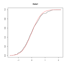
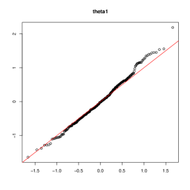
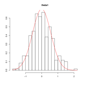
Figure 9: Simulation results of $\hat{\theta}_{1}$

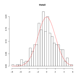
Figure 10: Simulation results of $\hat{\theta}_{0}$

5 Proofs

Proof of Theorem 2. Let $s_{i}=s_{i:N_{2}}$.

$$\check{\sigma}^{2}= \sum_{i=1}^{N_{2}}\left(\check{x}_{k}(s_{i})-\check{x}_{k}(s_{i-1})\right)^{2}$$

$$= \sum_{i=1}^{N_{2}}\left\{\check{x}_{k}(s_{i})-x_{k}(s_{i})-\{\check{x}_{k}(s_{i-1})-x_{k}(s_{i-1})\}+x_{k}(s_{i})-x_{k}(s_{i-1})\right\}^{2}$$

$$= \sum_{i=1}^{N_{2}}\left\{(\check{x}_{k}(s_{i})-x_{k}(s_{i}))^{2}\right.$$ (6)

$$+\left(\check{x}_{k}(s_{i-1})-x_{k}(s_{i-1})\right)^{2}$$ (7)

$$-2(\check{x}_{k}(s_{i})-x_{k}(s_{i}))(\check{x}_{k}(s_{i-1})-x_{k}(s_{i-1}))$$ (8)

$$+2\left\{\check{x}_{k}(s_{i})-x_{k}(s_{i})-\{\check{x}_{k}(s_{i-1})-x_{k}(s_{i-1})\}\right\}(x_{k}(s_{i})-x_{k}(s_{i-1}))$$ (9)

$$+\left.(x_{k}(s_{i})-x_{k}(s_{i-1}))^{2}\right\}.$$

First of all, we will show that

$$\sqrt{N_{2}}(\check{\sigma}^{2}-(\sigma^{*})^{2})-\sqrt{N_{2}}\left\{\sum_{i=1}^{N_{2}}(x_{k}(s_{i})-x_{k}(s_{i-1}))^{2}-(\sigma^{*})^{2}\right\}=o_{p}(1).$$ (10)

Let $g_{k}(t,y,\eta)=X_{t}(y)\sqrt{2}\sin(\pi ky)\exp\left\{\frac{\eta}{2}y\right\}$. Note that

$$x_{k}(t)= \int_{0}^{1}X_{t}(y)\sqrt{2}\sin(\pi ky)\exp\left\{\frac{\eta}{2}y\right\}dy=\sum_{j=1}^{M}\int_{\frac{j-1}{M}}^{\frac{j}{M}}g_{k}(t,y,\eta)dy,$$

$$\check{x}_{k}(t)= \frac{1}{M}\sum_{j=1}^{M}X_{t}(y_{j})\sqrt{2}\sin(\pi ky_{j})\exp\left\{\frac{\check{\eta}}{2}y_{j}\right\}=\frac{1}{M}\sum_{j=1}^{M}g_{k}(t,y_{j},\check{\eta}).$$

For the evaluation of (6) and (7), noting that

$$\left(\check{x}_{k}(s_{i})-x_{k}(s_{i})\right)^{2}= \left(M\frac{1}{M}\sum_{j=1}^{M}\int_{\frac{j-1}{M}}^{\frac{j}{M}}(g_{k}(s_{i},y,\eta)-g_{k}(s_{i},y_{j},\check{\eta})dy\right)^{2}$$

$$\leq M^{2}\frac{1}{M}\sum_{j=1}^{M}\left(\int_{\frac{j-1}{M}}^{\frac{j}{M}}1^{2}dy\right)\int_{\frac{j-1}{M}}^{\frac{j}{M}}\left(g_{k}(s_{i},y,\eta)-g_{k}(s_{i},y_{j},\check{\eta})\right)^{2}dy$$

$$= \sum_{j=1}^{M}\int_{\frac{j-1}{M}}^{\frac{j}{M}}\left(g_{k}(s_{i},y,\eta)-g_{k}(s_{i},y_{j},\check{\eta})\right)^{2}dy,$$

one has that

$${Z_{0}}:=\sqrt{N_{2}}\sum_{i=1}^{N_{2}}\left(\check{x}_{k}(s_{i})-x_{k}(s_{i})\right)^{2}\leq\sqrt{N_{2}}\sum_{i=1}^{N_{2}}\sum_{j=1}^{M}\int_{\frac{j-1}{M}}^{\frac{j}{M}}\left(g_{k}(s_{i},y,\eta)-g_{k}(s_{i},y_{j},\check{\eta})\right)^{2}dy.$$

It follows that

$$g_{k}(t,y,\eta)-g_{k}(t,y_{j},\check{\eta})= X_{t}(y)\sqrt{2}\sin(\pi ky)\exp\left\{\frac{\eta}{2}y\right\}-X_{t}(y_{j})\sqrt{2}\sin(\pi ky_{j})\exp\left\{\frac{\check{\eta}}{2}y_{j}\right\}$$

$$= (X_{t}(y)-X_{t}(y_{j}))\sqrt{2}\sin(\pi ky)\exp\left\{\frac{\eta}{2}y\right\}$$ (11)

$$+X_{t}(y_{j})\left(\sqrt{2}\sin(\pi ky)\exp\left\{\frac{\eta}{2}y\right\}-\sqrt{2}\sin(\pi ky_{j})\exp\left\{\frac{\eta}{2}y_{j}\right\}\right)$$ (12)

$$+X_{t}(y_{j})\sqrt{2}\sin(\pi ky_{j})\left\{\exp\left\{\frac{\eta}{2}y_{j}\right\}-\exp\left\{\frac{\check{\eta}}{2}y_{j}\right\}\right\}$$ (13)

$$=: g^{(1)}(t,y)+g^{(2)}(t,y)+g^{(3)}(t,y_{j},\check{\eta})$$

and that

$$Z_{0}\leq C\sqrt{N_{2}}\sum_{i=1}^{N_{2}}\sum_{j=1}^{M}\int_{\frac{j-1}{M}}^{\frac{j}{M}}\{(g^{(1)}(s_{i},y))^{2}+(g^{(2)}(s_{i},y))^{2}+(g^{(3)}(s_{i},y_{j},\check{\eta}))^{2}\}dy.$$

For the evaluation of (12), noting that

$$E\left[X_{t}^{2}(y)\right]= \sum_{k=1}^{\infty}\sum_{l=1}^{\infty}E[x_{k}(t)x_{l}(t)]e_{k}(y)e_{l}(y)$$

$$= \sum_{k=1}^{\infty}E[x_{k}^{2}(t)]e_{k}^{2}(y)=\sum_{k=1}^{\infty}\frac{\sigma^{2}}{2\lambda_{k}}\left\{1-e^{-2\lambda_{k}t}\right\}e_{k}^{2}(y)$$

$$\leq C\sum_{k=1}^{\infty}\frac{1}{k^{2}}<\infty$$

and

$$E[(g^{(2)}(s_{i},y))^{2}]\leq C(y_{j}-y_{j-1})^{2}\leq\frac{C}{M^{2}},$$

one has that under $\frac{N_{2}^{\frac{3}{2}}}{M^{1-\rho}}\rightarrow 0$,

$$\sqrt{N_{2}}N_{2}\frac{1}{N_{2}}\sum_{i=1}^{N_{2}}\sum_{j=1}^{M}\int_{\frac{j-1}{M}}^{\frac{j}{M}}(g^{(2)}(s_{i},y))^{2}dy=o_{p}(1).$$ (14)

For the evaluation of (13),

$$\sqrt{N_{2}}N_{2}\frac{1}{N_{2}}\sum_{i=1}^{N_{2}}\frac{1}{M}\sum_{j=1}^{M}(g^{(3)}(s_{i},y_{j},\check{\eta}))^{2}$$

$$= \sqrt{N_{2}}N_{2}\frac{1}{N_{2}}\sum_{i=1}^{N_{2}}\frac{1}{M}\sum_{j=1}^{M}X_{s_{i}}^{2}(y_{j}){2\sin^{2}(\pi ky_{j})\left(\int_{0}^{1}\frac{y_{j}}{2}\exp\left\{\frac{y_{j}}{2}(\eta+u(\check{\eta}-\eta))\right\}du\right)^{2}}\frac{1}{N_{m}}$$ (15)

$$\times(\sqrt{N_{m}}(\check{\eta}-\eta))^{2}.$$

Let $\zeta>0$ and $\epsilon>0$. On $A=\{|\check{\eta}-\eta|<\zeta\}$,

$$(\ref{thm2-A})\leq\frac{C}{N_{2}}\sum_{i=1}^{N_{2}}\frac{1}{M}\sum_{j=1}^{M}{X_{s_{i}}^{2}(y_{j})2\sin^{2}(\pi ky_{j})}\frac{N_{2}^{\frac{3}{2}}}{N_{m}},$$

and

$$P(|(\ref{thm2-A})|>\varepsilon)= P(\{|(\ref{thm2-A})|>\varepsilon\}\cap A)+P(\{|(\ref{thm2-A})|>\varepsilon\}\cap A^{c})$$

$$\leq P\left(\frac{N_{2}^{\frac{3}{2}}}{N_{m}}\frac{1}{N_{2}}\sum_{i=1}^{N_{2}}\frac{1}{M}\sum_{j=1}^{M}X_{s_{i}}^{2}(y_{j})2\sin^{2}(\pi y_{j})>\varepsilon\right)+P(A^{c})$$

$$\leq \frac{C}{\varepsilon}\frac{N_{2}^{\frac{3}{2}}}{N_{m}}+o(1)\rightarrow 0,$$

$$(\ref{thm2-A})= o_{p}(1).$$

Noting that $\sqrt{N_{m}}(\check{\eta}-\eta)=O_{p}(1)$, one has that under $\frac{N_{2}^{\frac{3}{2}}}{N_{m}}\rightarrow 0$,

$$\sqrt{N_{2}}\sum_{i=1}^{N_{2}}\frac{1}{M}\sum_{j=1}^{M}(g^{(3)}(s_{i},y_{j},\check{\eta}))^{2}=o_{p}(1).$$ (16)

For the evaluation of (11), noting that

$$E[(g^{(1)}(s_{i},y))^{2}]\leq CE\left[\left(X_{s_{i}}(y)-X_{s_{i}}(y_{j})\right)^{2}\right],$$

$$\left(X_{t}(y)-X_{t}(y_{j})\right)^{2}=\sum_{k,l}x_{k}(t)(e_{k}(y)-e_{l}(y_{j}))x_{l}(t)(e_{l}(y)-e_{l}(y_{j})),$$

$$|e_{k}(y)-e_{k}(y_{j})|$$

$$= \left|\int_{0}^{1}\left(\sqrt{2}\pi k\cos(\pi k(y_{j}+u(y-y_{j})))\exp\left\{-\frac{\eta}{2}(y_{j}+u(y-y_{j}))\right\}\right.\right.$$

$$+\left.\left.\sqrt{2}\sin(\pi k(y_{j}+u(y-y_{j})))\left(-\frac{\eta}{2}\right)\exp\left\{-\frac{\eta}{2}(y_{j}+u(y-y_{j}))\right\}\right)du\times(y-y_{j})\right|$$

$$\leq C\frac{k}{M},$$

$$E\left[\left(X_{t}(y)-X_{t}(y_{j})\right)^{2}\right]= \sum_{k=1}^{\infty}E[x_{k}^{2}(t)](e_{k}(y)-e_{k}(y_{j}))^{2}$$

$$\leq \sum_{k=1}^{\infty}\frac{C}{k^{2}}\left(\frac{k}{M}\right)^{1-\rho}C^{1+\rho}\leq\frac{C_{1}}{M^{1-\rho}},$$

we obtain that under $\frac{N_{2}^{\frac{3}{2}}}{M^{1-\rho}}\rightarrow 0$,

$$\sqrt{N_{2}}\sum_{i=1}^{N_{2}}\sum_{j=1}^{M}\int_{\frac{j-1}{M}}^{\frac{j}{M}}(g^{(1)}(s_{i},y))^{2}dy=O_{p}\left(\frac{N_{2}^{\frac{3}{2}}}{M^{1-\rho}}\right)=o_{p}(1).$$ (17)

Therefore, it follows from (14), (16) and (17) that under $\frac{N_{2}^{\frac{3}{2}}}{Nm}\rightarrow 0$ and $\frac{N_{2}^{\frac{3}{2}}}{M^{1-\rho}}\rightarrow 0$,

$$\sqrt{N_{2}}\sum_{i=1}^{N_{2}}\left(\check{x}_{k}(s_{i})-x_{k}(s_{i})\right)^{2}=o_{p}(1)$$

and

$$\sqrt{N_{2}}\sum_{i=1}^{N_{2}}\left(\check{x}_{k}(s_{i-1})-x_{k}(s_{i-1})\right)^{2}=o_{p}(1).$$

For the evaluation of (8), it follows that

$$\left|\sqrt{N_{2}}\sum_{i=1}^{N_{2}}\left(\check{x}_{k}(s_{i})-x_{k}(s_{i})\right)\left(\check{x}_{k}(s_{i-1})-x_{k}(s_{i-1})\right)\right|^{2}$$

$$\leq N_{2}\sum_{i=1}^{N_{2}}\left(\check{x}_{k}(s_{i})-x_{k}(s_{i})\right)^{2}\sum_{i=1}^{N_{2}}\left(\check{x}_{k}(s_{i-1})-x_{k}(s_{i-1})\right)^{2}$$

$$= \sqrt{N_{2}}\sum_{i=1}^{N_{2}}\left(\check{x}_{k}(s_{i})-x_{k}(s_{i})\right)^{2}\sqrt{N_{2}}\sum_{i=1}^{N_{2}}\left(\check{x}_{k}(s_{i-1})-x_{k}(s_{i-1})\right)^{2}$$

$$= o_{p}(1).$$

For the evaluation of (9), setting that $\Delta X_{s_{i}}(y)=X_{s_{i}}(y)-X_{s_{i-1}}(y)$ and $\Delta_{s_{i}}x=x_{1}(s_{i})-x_{1}(s_{i-1})$, one has that

$$U_{1}:= 2\sqrt{N_{2}}\sum_{i=1}^{N_{2}}\{\check{x}_{1}(s_{i})-\check{x}_{1}(s_{i-1})-(x_{1}(s_{i})-x_{1}(s_{i-1}))\}(x_{1}(s_{i})-x_{1}(s_{i-1}))$$

$$= 2\sqrt{N_{2}}\sum_{i=1}^{N_{2}}\frac{1}{M}\sum_{j=1}^{M}\Delta X_{s_{i}}(y_{j})\sqrt{2}\sin(\pi y_{j})\left(\exp\left\{\frac{\check{\eta}}{2}y_{j}\right\}-\exp\left\{\frac{\eta}{2}y_{j}\right\}\right)\times\Delta_{s_{i}}x$$ (18)

$$+2\sqrt{N_{2}}\sum_{i=1}^{N_{2}}\sum_{j=1}^{M}\int_{\frac{j-1}{M}}^{\frac{j}{M}}\Delta X_{s_{i}}(y_{j})(\sqrt{2}\sin(\pi y_{j})-\sqrt{2}\sin(\pi y))\exp\left\{\frac{\eta}{2}y_{j}\right\}dy\times\Delta_{s_{i}}x$$ (19)

$$+2\sqrt{N_{2}}\sum_{i=1}^{N_{2}}\sum_{j=1}^{M}\int_{\frac{j-1}{M}}^{\frac{j}{M}}\Delta X_{s_{i}}(y_{j})\sqrt{2}\sin(\pi y)\left(\exp\left\{\frac{\eta}{2}y_{j}\right\}-\exp\left\{\frac{\eta}{2}y\right\}\right)dy\times\Delta_{s_{i}}x$$ (20)

$$+2\sqrt{N_{2}}\sum_{i=1}^{N_{2}}\sum_{j=1}^{M}\int_{\frac{j-1}{M}}^{\frac{j}{M}}\left\{\Delta X_{s_{i}}(y_{j})-\Delta X_{s_{i}}(y)\right\}\sqrt{2}\sin(\pi y)\exp\left\{\frac{\eta}{2}y\right\}dy\times\Delta_{s_{i}}x.$$ (21)

For the evaluation of (18), noting that

$$(\ref{thm2-i})= 2\sqrt{N_{2}}\sum_{i=1}^{N_{2}}\frac{1}{M}\sum_{j=1}^{M}\Delta X_{s_{i}}(y_{j})\sqrt{2}\sin(\pi y_{j})\int_{0}^{1}\frac{y_{j}}{2}\exp\left\{\frac{y_{j}}{2}(\eta+u(\check{\eta}-\eta))\right\}du(\Delta_{s_{i}}x)(\check{\eta}-\eta),$$

one has that

$$(\ref{thm2-i})^{2}\leq 4N_{2}\sum_{i=1}^{N_{2}}\frac{1}{Nm}\frac{1}{M}\sum_{j=1}^{M}\left(\Delta X_{s_{i}}(y_{j})\right)^{2}\left(\sqrt{2}\sin(\pi y_{j})\int_{0}^{1}\frac{y_{j}}{2}\exp\left\{\frac{y_{j}}{2}(\eta+u(\check{\eta}-\eta))\right\}du\right)^{2}$$

$$\times\sum_{i=1}^{N_{2}}(\Delta_{s_{i}}x)^{2}\times(\sqrt{Nm}(\check{\eta}-\eta))^{2}.$$

Set that

$$B:= 4N_{2}\sum_{i=1}^{N_{2}}\frac{1}{Nm}\frac{1}{M}\sum_{j=1}^{M}\left(\Delta X_{s_{i}}(y_{j})\right)^{2}\left(\sqrt{2}\sin(\pi y_{j})\int_{0}^{1}\frac{y_{j}}{2}\exp\left\{\frac{y_{j}}{2}(\eta+u(\check{\eta}-\eta))\right\}du\right)^{2}.$$

Since

$$\sum_{i=1}^{N_{2}}(\Delta_{s_{i}}x)^{2}=O_{p}(1),\quad(\sqrt{Nm}(\check{\eta}-\eta))^{2}=O_{p}(1),$$

we obtain that

$$P(|B|>\varepsilon) =P(\{|B|>\varepsilon\}\cap A)+P(\{|B|>\varepsilon\}\cap A^{c})$$

$$\leq C\frac{N_{2}N_{2}}{Nm}E\left[\left(\Delta X_{s_{i}}(y_{j})\right)^{2}\right]\frac{1}{\varepsilon}+P(A^{c})$$

$$=C_{1}\frac{N_{2}^{\frac{3}{2}}}{Nm}\frac{1}{\varepsilon}+o(1)$$

$$\rightarrow 0$$

under $\frac{N_{2}^{\frac{3}{2}}}{Nm}\rightarrow 0$. Therefore $(\ref{thm2-i})^{2}=o_{p}(1)$.

For the evaluation of (19), noting that

$$N_{2}\sum_{i=1}^{N_{2}}\frac{1}{M}\sum_{j=1}^{M}\left(\Delta X_{s_{i}}(y_{j})\right)^{2}|y-y_{j}|^{2}=O_{p}\left(\frac{N_{2}^{2}}{\sqrt{N_{2}}M^{2}}\right),$$

$$\sum_{i=1}^{N_{2}}(\Delta_{s_{i}}x)^{2}=O_{p}(1),$$

one has that under $\frac{N_{2}^{\frac{3}{2}}}{M^{1-\rho}}\rightarrow 0$,

$$(\ref{thm2-ii})^{2}\leq N_{2}\sum_{i=1}^{N_{2}}\frac{1}{M}\sum_{j=1}^{M}\left(\Delta X_{s_{i}}(y_{j})\right)^{2}|y-y_{j}|^{2}\sum_{i=1}^{N_{2}}(\Delta_{s_{i}}x)^{2}=o_{p}(1).$$

For the evaluation of (20), noting that

$$N_{2}\sum_{i=1}^{N_{2}}M^{2}\frac{1}{M}\sum_{j=1}^{M}\frac{1}{M}\int_{\frac{j-1}{M}}^{\frac{j}{M}}\left(\Delta X_{s_{i}}(y_{j})\right)^{2}2\sin(\pi y)|y-y_{j}|^{2}dy=O_{p}\left(\frac{N_{2}^{2}}{\sqrt{N_{2}}M^{2}}\right),$$

$$\sum_{i=1}^{N_{2}}(\Delta_{s_{i}}x)^{2}=O_{p}(1),$$

we obtain that under $\frac{N_{2}^{\frac{3}{2}}}{M^{1-\rho}}\rightarrow 0$,

$$({\ref{thm2-iii}})^{2}\leq N_{2}\sum_{i=1}^{N_{2}}M^{2}\frac{1}{M}\sum_{j=1}^{M}\frac{1}{M}\int_{\frac{j-1}{M}}^{\frac{j}{M}}\left(\Delta X_{s_{i}}(y_{j})\right)^{2}2\sin(\pi y)|y-y_{j}|^{2}dy\sum_{i=1}^{N_{2}}(\Delta_{s_{i}}x)^{2}=o_{p}(1).$$

For the evaluation of (21), setting that

$$h(y,\Delta_{s_{i}}x):= \left(\sum_{k=1}^{\infty}(x_{k}(s_{i})-x_{k}(s_{i-1}))(e_{k}(y_{j})-e_{k}(y))\right)^{2}(x_{1}(s_{i})-x_{1}(s_{i-1}))^{2},$$

one has that

$$E[h(y,\Delta_{s_{i}}x)]= \sum_{k=2}^{\infty}E[(x_{k}(s_{i})-x_{k}(s_{i-1}))^{2}]E[(x_{1}(s_{i})-x_{1}(s_{i-1}))^{2}](e_{k}(y_{j})-e_{k}(y))^{2}$$

$$+E[(x_{1}(s_{i})-x_{1}(s_{i-1}))^{4}](e_{1}(y_{j})-e_{1}(y))^{2}$$

$$\leq \frac{C}{M^{1-\rho}}\frac{1}{N_{2}}+\frac{1}{N_{2}^{2}M^{2}}$$

and

$$({\ref{thm2-iv}})^{2}\leq N_{2}\sum_{i=1}^{N_{2}}M^{2}\frac{1}{M}\sum_{j=1}^{M}\frac{1}{M}\int_{\frac{j-1}{M}}^{\frac{j}{M}}h(y,\Delta_{s_{i}}x)dy.$$

Since it follows that under $\frac{N_{2}^{\frac{3}{2}}}{M^{1-\rho}}\rightarrow 0$,

$$E[(\ref{thm2-iv})^{2}]\leq\frac{N_{2}}{M^{1-\rho}}+\frac{1}{M^{2}}\rightarrow 0,$$

we obtain that $({\ref{thm2-iv}})=o_{p}(1)$. Hence, $U_{1}=o_{p}(1)$. Consequently, under $\frac{N_{2}^{\frac{3}{2}}}{N_{m}}\rightarrow 0$ and $\frac{N_{2}^{\frac{3}{2}}}{M^{1-\rho}}\rightarrow 0$, (10) holds true, which yields that

$$\sqrt{N_{2}}(\check{\sigma}^{2}-(\sigma^{*})^{2})\stackrel{{\scriptstyle d}}{{\rightarrow}}N\left(0,2(\sigma^{*})^{4}\right).$$ (22)

For the estimator of $\theta_{2}$, we obtain that

$$\sqrt{N_{2}}(\check{\theta}_{2}-\theta_{2}^{*}) = \sqrt{N_{2}}\left(\left(\frac{\check{\sigma}^{2}}{\check{\sigma}_{0}^{2}}\right)^{2}-\left(\frac{({\sigma^{*}})^{2}}{({\sigma_{0}^{*}})^{2}}\right)^{2}\right)$$

$$= \sqrt{N_{2}}\left(\check{\sigma}^{4}\left\{\left(\frac{1}{\check{\sigma}_{0}^{2}}\right)^{2}-\left(\frac{1}{({\sigma_{0}^{*}})^{2}}\right)^{2}\right\}+\frac{1}{(\sigma_{0}^{*})^{4}}\left\{\check{\sigma}^{4}-({\sigma^{*}})^{4}\right\}\right)$$

$$= \frac{\sqrt{N_{2}}}{\sqrt{mN}}\check{\sigma}^{4}\sqrt{mN}\left\{\left(\frac{1}{\check{\sigma}_{0}^{2}}\right)^{2}-\left(\frac{1}{({\sigma_{0}^{*}})^{2}}\right)^{2}\right\}+\sqrt{N_{2}}\frac{1}{(\sigma_{0}^{*})^{4}}\left\{\check{\sigma}^{4}-({\sigma^{*}})^{4}\right\}$$

$$= \sqrt{N_{2}}\frac{1}{(\sigma_{0}^{*})^{4}}\left\{\check{\sigma}^{4}-({\sigma^{*}})^{4}\right\}+o_{p}(1).$$

For the estimator of $\theta_{1}$, one has that

$$\sqrt{N_{2}}(\check{\theta}_{1}-\theta_{1}^{*}) = \sqrt{N_{2}}\left(\check{\eta}\hat{\theta}_{2}-\eta^{*}\theta_{2}^{*}\right)=\sqrt{N_{2}}\left(\check{\theta}_{2}\left(\check{\eta}-\eta^{*}\right)+\eta^{*}\left(\check{\theta}_{2}-\theta_{2}^{*}\right)\right)$$

$$= \sqrt{N_{2}}\eta^{*}\left(\check{\theta}_{2}-\theta_{2}^{*}\right)+o_{p}(1)$$

$$= \sqrt{N_{2}}\eta^{*}\frac{1}{(\sigma_{0}^{*})^{4}}\left\{\check{\sigma}^{4}-({\sigma^{*}})^{4}\right\}+o_{p}(1).$$

By noting that

$$\begin{pmatrix}\sqrt{N_{2}}(\check{\sigma}^{2}-(\sigma^{*})^{2})\\ \sqrt{N_{2}}(\check{\theta}_{2}-\theta_{2}^{*})\\ \sqrt{N_{2}}(\check{\theta}_{1}-\theta_{1}^{*})\end{pmatrix}=\begin{pmatrix}\sqrt{N_{2}}(\check{\sigma}^{2}-(\sigma^{*})^{2})\\ \sqrt{N_{2}}\frac{1}{(\sigma_{0}^{*})^{4}}(\check{\sigma}^{2}-(\sigma^{*})^{2})\\ \sqrt{N_{2}}\frac{\eta^{*}}{(\sigma_{0}^{*})^{4}}(\check{\sigma}^{2}-(\sigma^{*})^{2})\end{pmatrix}+o_{p}(1),$$

it follows from (22) and the delta method that under $\frac{N_{2}^{\frac{3}{2}}}{N_{m}}\rightarrow 0$ and $\frac{N_{2}^{\frac{3}{2}}}{M^{1-\rho}}\rightarrow 0$,

$$\begin{pmatrix}\sqrt{N_{2}}(\check{\sigma}^{2}-(\sigma^{*})^{2})\\ \sqrt{N_{2}}\frac{1}{(\sigma_{0}^{*})^{4}}(\check{\sigma}^{2}-(\sigma^{*})^{2})\\ \sqrt{N_{2}}\frac{\eta^{*}}{(\sigma_{0}^{*})^{4}}(\check{\sigma}^{2}-(\sigma^{*})^{2})\end{pmatrix}\stackrel{{\scriptstyle d}}{{\rightarrow}}N\left(\begin{pmatrix}0\\ 0\\ 0\end{pmatrix},\begin{pmatrix}2(\sigma^{*})^{4}&4\theta_{2}^{*}(\sigma^{*})^{2}&4\theta_{1}^{*}(\sigma^{*})^{2}\\ 4\theta_{2}^{*}(\sigma^{*})^{2}&8(\theta_{2}^{*})^{2}&8\theta_{1}^{*}\theta_{2}^{*}\\ 4\theta_{1}^{*}(\sigma^{*})^{2}&8\theta_{1}^{*}\theta_{2}^{*}&8(\theta_{1}^{*})^{2}\end{pmatrix}\right),$$

which completes the proof.

Proof of Theorem 3. By a similar way to the proof of Theorem 5.1 in Bibinger and Trabs (2007), we can show the result under $Nh_{N:T}^{2}\rightarrow 0$, $\bar{m}\rightarrow\infty$ and $\bar{m}=O(h_{N:T}^{-\rho})$ for $\rho\in(0,1/2)$.

Proof of Theorem 4. Let $\delta=\delta_{\bar{N}_{2}:T}$ and $s_{i}=s_{i:\bar{N}_{2}:T}$. The quasi log-likelihood function based on ${\bf\bar{x}}_{k}=\{\bar{x}_{k}(s_{i:\bar{N}_{2}:T})\}_{i=1,\ldots,\bar{N}_{2}}=\{\bar{x}_{k}(s_{i})\}_{i=1,\ldots,\bar{N}_{2}}$ is as follows.

$$l_{\bar{N}_{2}}(\lambda_{k},\sigma^{2}\ |\ {\bf\bar{x}}_{k})=-\frac{1}{2}\sum_{i=1}^{\bar{N}_{2}}\left\{\log\frac{\sigma^{2}(1-e^{-2\lambda_{k}\delta})}{2\lambda_{k}}+\frac{\left(\bar{x}_{k}(s_{i})-e^{-\lambda_{k}\delta}\bar{x}_{k}(s_{i-1})\right)^{2}}{\frac{\sigma^{2}(1-e^{-2\lambda_{k}\delta})}{2\lambda_{k}}}\right\}.$$

Set that $k=1$, $\lambda=\lambda_{1}$, ${\bf\bar{x}}={\bf\bar{x}}_{1}=\{\bar{x}_{1}(s_{i:\bar{N}_{2}:T})\}_{i=1,\ldots,\bar{N}_{2}}=\{\bar{x}_{1}(s_{i})\}_{i=1,\ldots,\bar{N}_{2}}$ and

$$\Xi(\lambda)=\frac{(1-e^{-2\lambda\delta})}{2\lambda\delta}.$$

For the consistency of $\hat{\sigma}_{2}$ and $\hat{\lambda}$, it is enough to show that under $\frac{\bar{N}_{2}^{\frac{5}{2}}}{T^{\frac{5}{2}}N\bar{m}}\to 0$ and $\frac{\bar{N}_{2}^{3}}{T^{3}M^{1-\rho_{1}}}\to 0$,

$$Z:=\frac{1}{T}\left\{l_{\bar{N}_{2}}(\lambda,\sigma^{2}\ |\ {\bf\bar{x}})-l_{\bar{N}_{2}}(\lambda,\sigma^{2}\ |\ {\bf{x}})\right\}=o_{p}(1)$$ (23)

uniformly in $(\lambda,\sigma^{2})$, where $Z$ is the difference between the quasi log-likelihood functions based on ${\bf\bar{x}}$ and ${\bf{x}}$. Note that (23) yields that

$$\frac{1}{\bar{N}_{2}}\left\{l_{\bar{N}_{2}}(\lambda,\sigma^{2}\ |\ {\bf\bar{x}})-l_{\bar{N}_{2}}(\lambda,\sigma^{2}\ |\ {\bf{x}})\right\}=o_{p}(1)$$

uniformly in $(\lambda,\sigma^{2})$.

Since

$$Z= \frac{1}{T}\frac{1}{2\sigma^{2}\delta\Xi(\lambda)}\sum_{i=1}^{\bar{N}_{2}}\left\{\left(\bar{x}_{1}(s_{i})-e^{-\lambda\delta}\bar{x}_{1}(s_{i-1})\right)^{2}\right.\left.-\left(x_{1}(s_{i})-e^{-\lambda\delta}x_{1}(s_{i-1})\right)^{2}\right\}$$

and

$$\left(\bar{x}_{1}(s_{i})-e^{-\lambda\delta}\bar{x}_{1}(s_{i-1})\right)^{2}$$

$$= \left\{\bar{x}_{1}(s_{i})-x_{1}(s_{i})-e^{-\lambda\delta}(\bar{x}_{1}(s_{i})-x_{1}(s_{i-1}))+(x_{1}(s_{i})-e^{-\lambda\delta}x_{1}(s_{i-1}))\right\}^{2}$$

$$= \left\{(\bar{x}_{1}(s_{i})-x_{1}(s_{i}))-e^{-\lambda\delta}(\bar{x}_{1}(s_{i-1})-x_{1}(s_{i-1}))\right\}^{2}$$

$$+2\{\bar{x}_{1}(s_{i})-x_{1}(s_{i})-e^{-\lambda\delta}(\bar{x}_{1}(s_{i-1})-x_{1}(s_{i-1}))\}(x_{1}(s_{i})-e^{-\lambda\delta}x_{1}(s_{i-1}))$$

$$+(x_{1}(s_{i})-e^{-\lambda\delta}x_{1}(s_{i-1}))^{2},$$

it follows that

$$Z= \frac{({\delta})^{-1}}{T}\frac{1}{2\sigma^{2}\Xi(\lambda)}\sum_{i=1}^{\bar{N}_{2}}\left[\left\{\left(\bar{x}_{1}(s_{i})-x_{1}(s_{i})\right)-e^{-\lambda\delta}\left(\bar{x}_{1}(s_{i-1})-x_{1}(s_{i-1})\right)\right\}^{2}\right.$$

$$\left.+2\left(\bar{x}_{1}(s_{i})-x_{1}(s_{i})\right)\left(x_{1}(s_{i})-e^{-\lambda\delta}x_{1}(s_{i-1})\right)\right.$$

$$\left.-2e^{-\lambda\delta}\left(\bar{x}_{1}(s_{i-1})-x_{1}(s_{i-1})\right)\left(x_{1}(s_{i})-e^{-\lambda\delta}x_{1}(s_{i-1})\right)\right]$$

$$= \frac{({\delta})^{-1}}{T}\frac{1}{2\sigma^{2}\Xi(\lambda)}\sum_{i=1}^{\bar{N}_{2}}\left[\left\{\left(\bar{x}_{1}(s_{i})-x_{1}(s_{i})\right)-e^{-\lambda\delta}\left(\bar{x}_{1}(s_{i-1})-x_{1}(s_{i-1})\right)\right\}^{2}\right.$$ (24)

$$\left.+2\left\{\bar{x}_{1}(s_{i})-\bar{x}_{1}(s_{i-1})-\left(x_{1}(s_{i})-x_{1}(s_{i-1})\right)\right\}\left(x_{1}(s_{i})-e^{-\lambda\delta}x_{1}(s_{i-1})\right)\right.$$ (25)

$$\left.+2(1-e^{-\lambda\delta})\left(\bar{x}_{1}(s_{i-1})-x_{1}(s_{i-1})\right)\left(x_{1}(s_{i})-e^{-\lambda\delta}x_{1}(s_{i-1})\right)\right]$$ (26)

$$=: W_{1}+W_{2}+W_{3}.$$

For the evaluation of (24), we set that

$$g_{1}(t,y,\eta) = X_{t}(y)\sqrt{2}\sin(\pi y)\exp\left\{\frac{\eta}{2}y\right\}.$$

Noting that

$$x_{1}(t) = \int_{0}^{1}X_{t}(y)\sqrt{2}\sin(\pi y)\exp\left\{\frac{\eta}{2}y\right\}dy=\int_{0}^{1}g_{1}(t,y,\eta)dy,$$

$$\bar{x}_{1}(t) = \frac{1}{M}\sum_{j=1}^{M}X_{t}(y_{j})\sqrt{2}\sin(\pi y_{j})\exp\left\{\frac{\hat{\eta}}{2}y_{j}\right\}=\frac{1}{M}\sum_{j=1}^{M}g_{1}(t,y_{j},\hat{\eta}),$$

we have that

$$Z_{1} := \frac{1}{T}\frac{1}{\delta}\sum_{i=1}^{\bar{N}_{2}}\left(x_{1}(s_{i})-\bar{x}_{1}(s_{i})\right)^{2}$$

$$= \frac{1}{T}\frac{1}{\delta}\sum_{i=1}^{\bar{N}_{2}}\left\{M\frac{1}{M}\sum_{j=1}^{M}\int_{\frac{j-1}{M}}^{\frac{j}{M}}\{g_{1}(s_{i},y,\eta)-g_{1}(s_{i},y_{j},\hat{\eta})\}dy\right\}^{2}$$

$$\leq \frac{1}{T}\frac{1}{\delta}\sum_{i=1}^{\bar{N}_{2}}M^{2}\frac{1}{M}\sum_{j=1}^{M}\frac{1}{M}\int_{\frac{j-1}{M}}^{\frac{j}{M}}\{g_{1}(s_{i},y,\eta)-g_{1}(s_{i},y_{j},\hat{\eta})\}^{2}dy$$

$$= \frac{1}{T}\frac{1}{\delta}\sum_{i=1}^{\bar{N}_{2}}\sum_{j=1}^{M}\int_{\frac{j-1}{M}}^{\frac{j}{M}}\{g_{1}(s_{i},y,\eta)-g_{1}(s_{i},y_{j},\hat{\eta})\}^{2}dy.$$

Moreover,

$$g_{1}(s_{i},y,\eta)-g_{1}(s_{i},y_{j},\hat{\eta})$$

$$= X_{s_{i}}(y)\sqrt{2}\sin(\pi y)\exp\left\{\frac{\eta}{2}y\right\}-X_{s_{i}}(y_{j})\sqrt{2}\sin(\pi y_{j})\exp\left\{\frac{\hat{\eta}}{2}y_{j}\right\}$$

$$= \left(X_{s_{i}}(y)-X_{s_{i}}(y_{j})\right)\sqrt{2}\sin(\pi y)\exp\left\{\frac{\eta}{2}y\right\}$$

$$+X_{s_{i}}(y_{j})\left(\sqrt{2}\sin(\pi y)\exp\left\{\frac{\eta}{2}y\right\}-\sqrt{2}\sin(\pi y_{j})\exp\left\{\frac{\eta}{2}y_{j}\right\}\right)$$

$$+X_{s_{i}}(y_{j})\sqrt{2}\sin(\pi y_{j})\left(\exp\left\{\frac{\eta}{2}y_{j}\right\}-\exp\left\{\frac{\hat{\eta}}{2}y_{j}\right\}\right).$$

$$= \bar{g}^{(1)}(s_{i},y)+\bar{g}^{(2)}(s_{i},y)+\bar{g}^{(3)}(s_{i},y_{j},\hat{\eta})$$

Set $R(y_{j},\hat{\eta}):=\int_{0}^{1}\frac{y_{j}}{2}\exp\left\{\frac{y_{j}}{2}(\eta+u(\hat{\eta}-\eta))\right\}du$. Let $\delta_{1}>0$. Since on $J=\{|\hat{\eta}-\eta|<\delta_{1}\}$

$$Z_{2}:=\frac{({\delta})^{-1}}{T}\sum_{i=1}^{\bar{N}_{2}}\frac{1}{M}\sum_{j=1}^{M}X_{s_{i}}^{2}(y_{j})2\sin^{2}(\pi y_{j})(R(y_{j},\hat{\eta}))^{2}\frac{1}{N\bar{m}}\leq C_{1}\frac{{\bar{N}_{2}}^{2}}{T^{2}}\frac{1}{N\bar{m}},$$

we obtain that

$$P(|Z_{2}|>\varepsilon) =P(|Z_{2}|>\varepsilon\cap J)+P(|Z_{2}|>\varepsilon\cap J^{c})\leq C_{1}\frac{{\bar{N}_{2}}^{2}}{T^{2}}\frac{1}{N\bar{m}}\frac{1}{\varepsilon}+o(1).$$ (30)

It follows that

$$E\left[(\bar{g}^{(1)}(s_{i},y))^{2}\times\frac{\bar{N}_{2}^{2}}{T^{2}}\right] \leq C_{1}E[\left(X_{s_{i}}(y)-X_{s_{i}}(y_{j})\right)^{2}]\frac{\bar{N}_{2}^{2}}{T^{2}}\leq\frac{C_{2}}{M^{1-\rho_{1}}}\frac{\bar{N}_{2}^{2}}{T^{2}},$$

$$E\left[(\bar{g}^{(2)}(s_{i},y))^{2}\times\frac{\bar{N}_{2}^{2}}{T^{2}}\right] \leq C_{1}(y-y_{j})^{2}\frac{\bar{N}_{2}^{2}}{T^{2}}\leq\frac{C_{1}}{M^{2}}\frac{\bar{N}_{2}^{2}}{T^{2}},$$

$$\frac{({\delta})^{-1}}{T}\sum_{i=1}^{\bar{N}_{2}}(\bar{g}^{(3)}(s_{i},y_{j},\hat{\eta}))^{2} = \frac{({\delta})^{-1}}{T}\sum_{i=1}^{\bar{N}_{2}}\frac{1}{M}\sum_{j=1}^{M}X_{s_{i}}^{2}(y_{j})2\sin^{2}(\pi y_{j})(R(y_{j},\hat{\eta}))^{2}\frac{1}{N\bar{m}}\left(\sqrt{N\bar{m}}(\hat{\eta}-\eta)\right)^{2}$$

$$= Z_{2}\left(\sqrt{N\bar{m}}(\hat{\eta}-\eta)\right)^{2}=O_{p}\left(\frac{{\bar{N}_{2}}^{2}}{T^{2}}\frac{1}{N\bar{m}}\right),$$

where we use (30) for the last estimate.

Hence

$$Z_{1} = O_{p}\left(\frac{{\bar{N}_{2}}^{2}}{T^{2}M^{1-\rho_{1}}}\right)+O_{p}\left(\frac{{\bar{N}_{2}}^{2}}{T^{2}N\bar{m}}\right),$$

$$W_{1} = O_{p}\left(\frac{{\bar{N}_{2}}^{2}}{T^{2}M^{1-\rho_{1}}}\right)+O_{p}\left(\frac{{\bar{N}_{2}}^{2}}{T^{2}N\bar{m}}\right).$$

For the evaluation of (26), one has that

$$W_{3}^{2}\leq C\frac{({\delta})^{-1}}{T}({\delta})^{2}\frac{({\delta})^{-1}}{T}\sum_{i=1}^{\bar{N}_{2}}\left(\bar{x}_{1}(s_{i})-x_{1}(s_{i-1})\right)^{2}\sum_{i=1}^{\bar{N}_{2}}\left(x_{1}(s_{i})-e^{-\lambda\delta}x_{1}(s_{i-1})\right)^{2}$$

$$= \frac{T}{\bar{N}_{2}}\times\left(O_{p}\left(\frac{{\bar{N}_{2}}^{2}}{T^{2}M^{1-\rho_{1}}}\right)+O_{p}\left(\frac{{\bar{N}_{2}}^{2}}{T^{2}N\bar{m}}\right)\right)$$

$$= O_{p}\left(\frac{{\bar{N}_{2}}}{TM^{1-\rho_{1}}}\right)+O_{p}\left(\frac{{\bar{N}_{2}}}{TN\bar{m}}\right).$$

For the evaluation of (25), setting that $\Delta X_{s_{i}}(y)=X_{s_{i}}(y)-X_{s_{i-1}}(y)$, we obtain that

$$\frac{({\delta})^{-1}}{T}\sum_{i=1}^{\bar{N}_{2}}\left\{\bar{x}_{1}(s_{i})-\bar{x}_{1}(s_{i-1})-\left(x_{1}(s_{i})-x_{1}(s_{i-1})\right)\right\}\left(x_{1}(s_{i})-e^{-\lambda\delta}x_{1}(s_{i-1})\right)$$

$$=\frac{({\delta})^{-1}}{T}\sum_{i=1}^{\bar{N}_{2}}\frac{1}{M}\sum_{j=1}^{M}\Delta X_{s_{i}}(y_{j})\sqrt{2}\sin(\pi y_{j})\left(\exp\left\{\frac{\hat{\eta}}{2}y_{j}\right\}-\exp\left\{\frac{\eta}{2}y_{j}\right\}\right)\left(x_{1}(s_{i})-e^{-\lambda\delta}x_{1}(s_{i-1})\right)$$

$$+\frac{({\delta})^{-1}}{T}\sum_{i=1}^{\bar{N}_{2}}\sum_{j=1}^{M}\int_{\frac{j-1}{M}}^{\frac{j}{M}}\Delta X_{s_{i}}(y_{j})\left(\sqrt{2}\sin(\pi y_{j})-\sqrt{2}\sin(\pi y)\right)\exp\left\{\frac{\eta}{2}y_{j}\right\}dy\left(x_{1}(s_{i})-e^{-\lambda\delta}x_{1}(s_{i-1})\right)$$

$$+\frac{({\delta})^{-1}}{T}\sum_{i=1}^{\bar{N}_{2}}\sum_{j=1}^{M}\int_{\frac{j-1}{M}}^{\frac{j}{M}}\Delta X_{s_{i}}(y_{j})\sqrt{2}\sin(\pi y)\left(\exp\left\{\frac{\eta}{2}y_{j}\right\}-\exp\left\{\frac{\eta}{2}y\right\}\right)dy\left(x_{1}(s_{i})-e^{-\lambda\delta}x_{1}(s_{i-1})\right)$$

$$+\frac{({\delta})^{-1}}{T}\sum_{i=1}^{\bar{N}_{2}}\sum_{j=1}^{M}\int_{\frac{j-1}{M}}^{\frac{j}{M}}\left\{\Delta X_{s_{i}}(y_{j})-\Delta X_{s_{i}}(y)\right\}\sqrt{2}\sin(\pi y)\exp\left\{\frac{\eta}{2}y\right\}dy\left(x_{1}(s_{i})-e^{-\lambda\delta}x_{1}(s_{i-1})\right)$$

$$=:\ ({\rm I})+({\rm II})+({\rm III})+({\rm IV}).$$

For the evaluation of (I), one has that

$$({\rm I})^{2}\leq \left(\frac{({\delta})^{-1}}{T}\right)^{2}\sum_{i=1}^{\bar{N}_{2}}\frac{1}{M}\sum_{j=1}^{M}\left(\Delta X_{s_{i}}(y_{j})\right)^{2}\left(\sqrt{2}\sin(\pi y_{j})R(y_{j},\hat{\eta})\right)^{2}\frac{T}{N\bar{m}}$$ (31)

$$\times\frac{1}{T}\sum_{i=1}^{\bar{N}_{2}}\left(x_{1}(s_{i})-e^{-\lambda\delta}x_{1}(s_{i-1})\right)^{2}\times\left(\sqrt{N\bar{m}}(\hat{\eta}-\eta)\right)^{2}.$$

Let $\eta_{1}>0$ and $\epsilon>0$. On $J=\{|\hat{\eta}-\eta|<\eta_{1}\}$,

$$(\ref{Z-C1})\leq C_{1}\frac{({\delta})^{-2}}{N\bar{m}}\frac{1}{T}\sum_{i=1}^{\bar{N}_{2}}\frac{1}{M}\sum_{j=1}^{M}\left(X_{s_{i}}(y_{j})-X_{s_{i-1}}(y_{j})\right)^{2}=O_{p}\left({\frac{1}{\delta^{\frac{5}{2}}N\bar{m}}}\right)=O_{p}\left({\frac{{\bar{N}_{2}}^{\frac{5}{2}}}{T^{\frac{5}{2}}N\bar{m}}}\right)$$

because $E\left[\left(\Delta X_{s_{i}}(y_{j})\right)^{2}\right]=\sqrt{{\delta}}=\sqrt{T/\bar{N}_{2}}$. It follows that under $\frac{\bar{N}_{2}^{\frac{5}{2}}}{T^{\frac{5}{2}}N\bar{m}}\to 0$,

$$P(|(\ref{Z-C1})|>\varepsilon) =P(|(\ref{Z-C1})|>\varepsilon\cap J)+P(|(\ref{Z-C1})|>\varepsilon\cap J^{c})\leq{\frac{{\bar{N}_{2}}^{\frac{5}{2}}}{T^{\frac{5}{2}}N\bar{m}}}\frac{1}{\varepsilon}+o(1)\rightarrow 0.$$

Therefore, $({\rm I})=o_{p}(1)$.

For the evaluation of (II), we obtain that

$$({\rm II})^{2}\leq C_{1}\left(\frac{{\delta}^{-1}}{T}\right)^{2}\sum_{i=1}^{\bar{N}_{2}}\frac{1}{M}\sum_{j=1}^{M}\left(\Delta X_{s_{i}}(y_{j})\right)^{2}|y-y_{j}|^{2}\sum_{i=1}^{\bar{N}_{2}}\left(x_{1}(s_{i})-e^{-\lambda\delta}x_{1}(s_{i-1})\right)^{2}$$

$$= O_{p}\left(\left(\frac{\bar{N}_{2}}{T^{2}}\right)^{2}\bar{N}_{2}\sqrt{\frac{T}{\bar{N}_{2}}}\frac{1}{M^{2}}T\right)=O_{p}\left(\frac{{\bar{N}_{2}}^{\frac{5}{2}}}{T^{\frac{5}{2}}M^{2}}\right).$$

For the evaluation of (III), one has that

$$({\rm III})^{2}\leq C_{1}\left(\frac{{\delta}^{-1}}{T}\right)^{2}\sum_{i=1}^{\bar{N}_{2}}\frac{1}{M}\sum_{j=1}^{M}\left(\Delta X_{s_{i}}(y_{j})\right)^{2}|y-y_{j}|^{2}\sum_{i=1}^{\bar{N}_{2}}\left(x_{1}(s_{i})-e^{-\lambda\delta}x_{1}(s_{i-1})\right)^{2}$$

$$= O_{p}\left(\frac{{\bar{N}_{2}}^{\frac{5}{2}}}{T^{\frac{5}{2}}M^{2}}\right).$$

For the evaluation of (IV), we obtain that

$$({\rm IV})^{2} \leq \left(\frac{{\delta}^{-1}}{T}\right)^{2}{\bar{N}_{2}}\sum_{i=1}^{\bar{N}_{2}}M^{2}\frac{1}{M}$$

$$\times\sum_{j=1}^{M}\frac{1}{M}\int_{\frac{j-1}{M}}^{\frac{j}{M}}\left(\left(\sum_{k=1}^{\infty}(x_{k}(s_{i})-x_{k}(s_{i-1}))(e_{k}(y_{j})-e_{k}(y))\right)^{2}(x_{1}(s_{i})-{e^{-\lambda\delta}}x_{1}(s_{i-1}))^{2}\right)dy.$$

By setting that

$$Z_{3}:=\left(\sum_{k=1}^{\infty}(x_{k}(s_{i})-x_{k}(s_{i-1}))(e_{k}(y_{j})-e_{k}(y))\right)^{2}(x_{1}(s_{i})-{e^{-\lambda\delta}}x_{1}(s_{i-1}))^{2},$$

it follows that

$$E[Z_{3}]= \sum_{k=2}^{\infty}E[(x_{k}(s_{i})-x_{k}(s_{i-1}))^{2}]E[(x_{1}(s_{i})-{e^{-\lambda\delta}}x_{1}(s_{i-1}))^{2}](e_{k}(y_{j})-e_{k}(y))^{2}$$

$$+E[{(x_{1}(s_{i})-x_{1}(s_{i-1}))^{2}(x_{1}(s_{i})-e^{-\lambda\delta}x_{1}(s_{i-1}))^{2}}](e_{1}(y_{j})-e_{1}(y))^{2}$$

$$\leq C_{1}\left(\frac{1}{M^{1-\rho_{1}}}\delta+\frac{{\delta}^{2}}{M^{2}}\right).$$

Therefore, under $\frac{\bar{N}_{2}^{3}}{T^{3}M^{1-\rho_{1}}}\to 0$,

$$E[({\rm IV})^{2}]\leq \frac{{\delta}^{-2}}{T^{2}}{\bar{N}_{2}^{2}}\cdot\frac{\delta}{M^{1-\rho_{1}}}=\frac{{\bar{N}_{2}^{3}}}{T^{3}M^{1-\rho_{1}}}\rightarrow 0.$$

Consequently, under $\frac{\bar{N}_{2}^{\frac{5}{2}}}{T^{\frac{5}{2}}N\bar{m}}\to 0$ and $\frac{\bar{N}_{2}^{3}}{T^{3}M^{1-\rho_{1}}}\to 0$, one has that $W_{2}=o_{p}(1)$ and

$$\frac{1}{T}\left\{l_{\bar{N}_{2}}(\lambda,\sigma^{2}\ |\ {\bf\bar{x}})-l_{\bar{N}_{2}}(\lambda,\sigma^{2}\ |\ {\bf{x}})\right\}=o_{p}(1)$$

uniformly in $(\lambda,\sigma^{2})$, which completes the proof of consistency of $(\hat{\lambda},\check{\sigma}^{2})$.

Next, we will show the asymptotic normality of $(\hat{\lambda},\check{\sigma}^{2})$. The derivatives of the quasi log-likelihood function with respect to the parameters are as follows.

$$\partial_{\lambda}l_{\bar{N}_{2}}(\lambda,\sigma^{2}\ |\ {\bf\bar{x}})= -\frac{1}{2}\sum_{i=1}^{\bar{N}_{2}}\left\{\frac{\partial_{\lambda}\Xi(\lambda)}{\Xi(\lambda)}-\frac{(\partial_{\lambda}\Xi(\lambda))\left(\bar{x}_{1}(s_{i})-e^{-\lambda\delta}\bar{x}_{1}(s_{i-1})\right)^{2}}{\sigma^{2}\Xi(\lambda)^{2}\delta}\right.$$

$$\left.+\frac{2\delta e^{-\lambda\delta}\bar{x}_{1}(s_{i-1})\left(\bar{x}_{1}(s_{i})-e^{-\lambda\delta}\bar{x}_{1}(s_{i-1})\right)}{\sigma^{2}\Xi(\lambda)\delta}\right\}.$$

$$\partial_{\sigma^{2}}l_{\bar{N}_{2}}(\lambda,\sigma^{2}\ |\ {\bf\bar{x}})=-\frac{1}{2}\sum_{i=1}^{\bar{N}_{2}}\left\{\frac{1}{\sigma^{2}}-\frac{1}{\sigma^{4}}\frac{\left(\bar{x}_{1}(s_{i})-e^{-\lambda\delta}\bar{x}_{1}(s_{i-1})\right)^{2}}{\Xi(\lambda)\delta}\right\}.$$

$$\partial_{\lambda}^{2}l_{\bar{N}_{2}}(\lambda,\sigma^{2}\ |\ {\bf\bar{x}})= -\frac{1}{2}\sum_{i=1}^{\bar{N}_{2}}\left\{\partial_{\lambda}\left(\frac{\partial_{\lambda}\Xi(\lambda)}{\Xi(\lambda)}\right)-\partial_{\lambda}\left(\frac{\partial_{\lambda}\Xi(\lambda)}{\Xi(\lambda)^{2}}\right)\frac{\left(\bar{x}_{1}(s_{i})-e^{-\lambda\delta}\bar{x}_{1}(s_{i-1})\right)^{2}}{\sigma^{2}\delta}\right.$$

$$\left.+\left(\frac{\partial_{\lambda}\Xi(\lambda)}{\Xi(\lambda)^{2}}\right)\frac{2\delta e^{-\lambda\delta}\bar{x}_{1}(s_{i-1})\left(\bar{x}_{1}(s_{i})-e^{-\lambda\delta}\bar{x}_{1}(s_{i-1})\right)}{\sigma^{2}\delta}\right.$$

$$\left.-\frac{\partial_{\lambda}\Xi(\lambda)}{\Xi(\lambda)^{2}}\frac{2\delta e^{-\lambda\delta}\bar{x}_{1}(s_{i-1})\left(\bar{x}_{1}(s_{i})-e^{-\lambda\delta}\bar{x}_{1}(s_{i-1})\right)}{\sigma^{2}\delta}\right.$$

$$\left.-\frac{1}{\Xi(\lambda)}\frac{2{\delta}^{2}e^{-\lambda\delta}\bar{x}_{1}(s_{i-1})\left(\bar{x}_{1}(s_{i})-e^{-\lambda\delta}\bar{x}_{1}(s_{i-1})\right)}{\sigma^{2}\delta}\right.$$

$$\left.-\frac{1}{\Xi(\lambda)}\frac{2{\delta}^{2}e^{-2\lambda\delta}\bar{x}_{1}^{2}(s_{i-1})}{\sigma^{2}\delta}\right\}.$$

$$\partial_{\sigma^{2}}^{2}l_{\bar{N}_{2}}(\lambda,\sigma^{2}\ |\ {\bf\bar{x}})=-\frac{1}{2}\sum_{i=1}^{\bar{N}_{2}}\left\{\frac{-1}{\sigma^{4}}+\frac{2}{\sigma^{6}}\frac{\left(\bar{x}_{1}(s_{i})-e^{-\lambda\delta}\bar{x}_{1}(s_{i-1})\right)^{2}}{\Xi(\lambda)\delta}\right\}.$$

$$\partial_{\lambda}\partial_{\sigma^{2}}l_{\bar{N}_{2}}(\lambda,\sigma^{2}\ |\ {\bf\bar{x}})= -\frac{1}{2}\sum_{i=1}^{\bar{N}_{2}}\left\{\frac{-1}{\sigma^{4}}\frac{-\partial_{\lambda}\Xi(\lambda)}{\Xi(\lambda)^{2}}\frac{\left(\bar{x}_{1}(s_{i})-e^{-\lambda\delta}\bar{x}_{1}(s_{i-1})\right)^{2}}{\delta}\right.$$

$$\left.+\frac{-1}{\sigma^{4}}\frac{1}{\Xi(\lambda)}\frac{2\delta e^{-\lambda\delta}\bar{x}_{1}(s_{i-1})\left(\bar{x}_{1}(s_{i})-e^{-\lambda\delta}\bar{x}_{1}(s_{i-1})\right)}{\delta}\right\}.$$

The difference between the score function of the volatility parameter $\sigma^{2}$ based on ${\bf\bar{x}}$ and that based on ${\bf{x}}$ is as follows.

$$\frac{1}{\sqrt{\bar{N}_{2}}}\left\{\partial_{\sigma^{2}}l_{\bar{N}_{2}}(\lambda,\sigma^{2}\ |\ {\bf\bar{x}})-\partial_{\sigma^{2}}l_{\bar{N}_{2}}(\lambda,\sigma^{2}\ |\ {\bf{x}})\right\}$$

$$= \frac{1}{\sqrt{\bar{N}_{2}}}\frac{1}{2\sigma^{4}\delta\Xi(\lambda)}\sum_{i=1}^{\bar{N}_{2}}\left\{\left(\bar{x}_{1}(s_{i})-e^{-\lambda\delta}\bar{x}_{1}(s_{i-1})\right)^{2}\right.\left.-\left(x_{1}(s_{i})-e^{-\lambda\delta}x_{1}(s_{i-1})\right)^{2}\right\}.$$

By an analogous manner to (23), it is shown that under $\frac{\bar{N}_{2}^{\frac{3}{2}}}{T^{\frac{1}{2}}N\bar{m}}\to 0$ and $\frac{\bar{N}_{2}^{2}}{TM^{1-\rho_{1}}}\to 0$,

$$\frac{1}{\sqrt{\bar{N}_{2}}}\left\{\partial_{\sigma^{2}}l_{\bar{N}_{2}}(\lambda,\sigma^{2}\ |\ {\bf\bar{x}})-\partial_{\sigma^{2}}l_{\bar{N}_{2}}(\lambda,\sigma^{2}\ |\ {\bf{x}})\right\}=o_{p}(1)$$

uniformly in $(\lambda,\sigma^{2})$.

The difference between the score function of the drift parameter $\lambda$ based on ${\bf\bar{x}}$ and that based on ${\bf{x}}$ is as follows.

$$F:= \frac{1}{\sqrt{T}}\left\{\partial_{\lambda}l_{\bar{N}_{2}}(\lambda,\sigma^{2}\ |\ {\bf\bar{x}})-\partial_{\lambda}l_{\bar{N}_{2}}(\lambda,\sigma^{2}\ |\ {\bf{x}})\right\}$$

$$= \left(-\frac{1}{2}\right)\frac{1}{\sqrt{T}}\sum_{i=1}^{\bar{N}_{2}}\left[\left(-\frac{\partial_{\lambda}\Xi(\lambda)}{\sigma^{2}\Xi(\lambda)^{2}}\right)\left\{\left(\bar{x}_{1}(s_{i})-e^{-\lambda\delta}\bar{x}_{1}(s_{i-1})\right)^{2}-\left(x_{1}(s_{i})-e^{-\lambda\delta}x_{1}(s_{i-1})\right)^{2}\right\}{\delta}^{-1}\right.$$

$$+2\left.\frac{e^{-\lambda\delta}}{\sigma^{2}\Xi(\lambda)}\left\{\bar{x}_{1}(s_{i})\left(\bar{x}_{1}(s_{i})-e^{-\lambda\delta}\bar{x}_{1}(s_{i-1})\right)-x_{1}(s_{i})\left(x_{1}(s_{i})-e^{-\lambda\delta}x_{1}(s_{i-1})\right)\right\}\right]$$

$$=: F_{1}+F_{2}.$$

By a similar way to (23), one has that under $\frac{\bar{N}_{2}^{\frac{5}{2}}}{T^{\frac{3}{2}}N\bar{m}}\to 0$ and $\frac{\bar{N}_{2}^{3}}{T^{2}M^{1-\rho_{1}}}\to 0$,

$$F_{1} =o_{p}(1).$$

For the evaluation of $F_{2}$, one has that

$$F_{2}= \left(\frac{-1}{\sqrt{T}}\right)\frac{e^{-\lambda\delta}}{\sigma^{2}\Xi(\lambda)}\sum_{i=1}^{\bar{N}_{2}}\left[\left(\bar{x}_{1}(s_{i})-x_{1}(s_{i})\right)\left(\bar{x}_{1}(s_{i})-e^{-\lambda\delta}\bar{x}_{1}(s_{i-1})\right)\right.$$

$$+\left.x_{1}(s_{i})\left\{\bar{x}_{1}(s_{i})-x_{1}(s_{i})-e^{-\lambda\delta}(\bar{x}_{1}(s_{i-1})-x_{1}(s_{i-1}))\right\}\right]$$

$$= \left(\frac{-1}{\sqrt{T}}\right)\frac{e^{-\lambda\delta}}{\sigma^{2}\Xi(\lambda)}\sum_{i=1}^{\bar{N}_{2}}\left[\left(\bar{x}_{1}(s_{i})-x_{1}(s_{i})\right)\left\{\bar{x}_{1}(s_{i})-x_{1}(s_{i})-e^{-\lambda\delta}({\bar{x}_{1}(s_{i-1})}-x_{1}(s_{i-1})\right\}\right.$$

$$+\left(\bar{x}_{1}(s_{i})-x_{1}(s_{i})\right)\left(x_{1}(s_{i})-e^{-\lambda\delta}x_{1}(s_{i-1})\right)$$

$$+\left.x_{1}(s_{i})\left\{\bar{x}_{1}(s_{i})-x_{1}(s_{i})-e^{-\lambda\delta}(\bar{x}_{1}(s_{i-1})-x_{1}(s_{i-1}))\right\}\right]$$

$$= \left(\frac{-1}{\sqrt{T}}\right)\frac{e^{-\lambda\delta}}{\sigma^{2}\Xi(\lambda)}\sum_{i=1}^{\bar{N}_{2}}\left[\left(\bar{x}_{1}(s_{i})-x_{1}(s_{i})\right)^{2}\right.\hskip 184.9429pt$$ (32)

$$-\left.e^{-\lambda\delta}\left(\bar{x}_{1}(s_{i})-x_{1}(s_{i})\right)\left(\bar{x}_{1}(s_{i-1})-x_{1}(s_{i-1})\right)\right.$$ (33)

$$+\left.\left(\bar{x}_{1}(s_{i})-x_{1}(s_{i})\right)\left(x_{1}(s_{i})-e^{-\lambda\delta}x_{1}(s_{i-1})\right)\right\}.$$ (34)

$$+\left.x_{1}(s_{i})\left\{\bar{x}_{1}(s_{i})-x_{1}(s_{i})-e^{-\lambda\delta}(\bar{x}_{1}(s_{i-1})-x_{1}(s_{i-1}))\right\}\right]$$ (35)

$$=: H_{1}+H_{2}+H_{3}+H_{4}.$$

For the evaluation of (32), it follows from the evaluation of (24) that

$$\frac{1}{\sqrt{T}\sqrt{\delta}}\sum_{i=1}^{\bar{N}_{2}}\left(\bar{x}_{1}(s_{i})-x_{1}(s_{i})\right)^{2}=O_{p}\left(\frac{{\bar{N}_{2}}^{\frac{3}{2}}}{TM^{1-\rho_{1}}}\right)+O_{p}\left(\frac{{\bar{N}_{2}}^{\frac{3}{2}}}{TN\bar{m}}\right)$$

and that under $\frac{\bar{N}_{2}^{\frac{5}{2}}}{T^{\frac{3}{2}}N\bar{m}}\to 0$ and $\frac{\bar{N}_{2}^{3}}{T^{2}M^{1-\rho_{1}}}\to 0$,

$$|H_{1}| \leq C_{1}\frac{1}{\sqrt{T}}\sum_{i=1}^{\bar{N}_{2}}\left(\bar{x}_{1}(s_{i})-x_{1}(s_{i})\right)^{2}=O_{p}\left(\frac{{\bar{N}_{2}}}{\sqrt{T}M^{1-\rho_{1}}}\right)+O_{p}\left(\frac{{\bar{N}_{2}}}{\sqrt{T}N\bar{m}}\right)\stackrel{{\scriptstyle p}}{{\rightarrow}}0.$$

For the evaluation of (33), we obtain that under $\frac{\bar{N}_{2}^{\frac{5}{2}}}{T^{\frac{3}{2}}N\bar{m}}\to 0$ and $\frac{\bar{N}_{2}^{3}}{T^{2}M^{1-\rho_{1}}}\to 0$,

$$H_{2}^{2} \leq\frac{1}{T}\sum_{i=1}^{\bar{N}_{2}}\left(\bar{x}_{1}(s_{i})-x_{1}(s_{i})\right)^{2}\sum_{i=1}^{\bar{N}_{2}}\left(\bar{x}_{1}(s_{i-1})-x_{1}(s_{i-1})\right)^{2}$$

$$=O_{p}\left(\left(\frac{\bar{N}_{2}}{\sqrt{T}M^{1-\rho_{1}}}\right)^{2}\right)+O_{p}\left(\left(\frac{\bar{N}_{2}}{\sqrt{T}N\bar{m}}\right)^{2}\right)\stackrel{{\scriptstyle p}}{{\rightarrow}}0.$$

For the evaluation of (34), setting that

$$\Delta x(s_{i},s_{i-1})=x_{1}(s_{i})-e^{-\lambda\delta}x_{1}(s_{i-1}),$$

one has that

$$-H_{3}=\frac{1}{\sqrt{T}}\frac{e^{-\lambda\delta}}{\sigma^{2}\Xi(\lambda)}\sum_{i=1}^{\bar{N}_{2}}\left\{\left(\bar{x}_{1}(s_{i})-x_{1}(s_{i})\right)\left(x_{1}(s_{i})-e^{-\lambda\delta}x_{1}(s_{i-1})\right)\right\}$$

$$=\frac{1}{\sqrt{T}}\frac{e^{-\lambda\delta}}{\sigma^{2}\Xi(\lambda)}\sum_{i=1}^{\bar{N}_{2}}\frac{1}{M}\sum_{j=1}^{M}X_{s_{i}}(y_{j})\sqrt{2}\sin(\pi y_{j})\left(\exp\left\{\frac{\hat{\eta}}{2}y_{j}\right\}-\exp\left\{\frac{\eta}{2}y_{j}\right\}\right)\Delta x(s_{i},s_{i-1})$$ (36)

$$+\frac{1}{\sqrt{T}}\frac{e^{-\lambda\delta}}{\sigma^{2}\Xi(\lambda)}\sum_{i=1}^{\bar{N}_{2}}\sum_{j=1}^{M}\int_{\frac{j-1}{M}}^{\frac{j}{M}}X_{s_{i}}(y_{j})\left(\sqrt{2}\sin(\pi y_{j})-\sqrt{2}\sin(\pi y)\right)\exp\left\{\frac{\eta}{2}y_{j}\right\}dy\Delta x(s_{i},s_{i-1})$$ (37)

$$+\frac{1}{\sqrt{T}}\frac{e^{-\lambda\delta}}{\sigma^{2}\Xi(\lambda)}\sum_{i=1}^{\bar{N}_{2}}\sum_{j=1}^{M}\int_{\frac{j-1}{M}}^{\frac{j}{M}}X_{s_{i}}(y_{j})\sqrt{2}\sin(\pi y)\left(\exp\left\{\frac{\eta}{2}y_{j}\right\}-\exp\left\{\frac{\eta}{2}y\right\}\right)dy\Delta x(s_{i},s_{i-1})$$ (38)

$$+\frac{1}{\sqrt{T}}\frac{e^{-\lambda\delta}}{\sigma^{2}\Xi(\lambda)}\sum_{i=1}^{\bar{N}_{2}}\sum_{j=1}^{M}\int_{\frac{j-1}{M}}^{\frac{j}{M}}\left(X_{s_{i}}(y_{j})-X_{s_{i}}(y)\right)\sqrt{2}\sin(\pi y)\exp\left\{\frac{\eta}{2}y\right\}dy\Delta x(s_{i},s_{i-1}).$$ (39)

For the evaluation of (36), it follows that under $\frac{\bar{N}_{2}^{\frac{5}{2}}}{T^{\frac{3}{2}}N\bar{m}}\to 0$,

$$(\ref{est-1})^{2}\leq \frac{1}{T}\sum_{i=1}^{\bar{N}_{2}}\frac{1}{M}\sum_{j=1}^{M}\left(X_{s_{i}}(y_{j})\sqrt{2}\sin(\pi y_{j})R(y_{j},\hat{\eta})(\hat{\eta}-\eta)\right)^{2}\sum_{i=1}^{\bar{N}_{2}}(\Delta x(s_{i},s_{i-1}))^{2}$$

$$= O_{p}\left(\frac{\bar{N}_{2}}{N\bar{m}}\right)\stackrel{{\scriptstyle p}}{{\rightarrow}}0.$$

For the evaluation of (37), one has that under $\frac{\bar{N}_{2}^{3}}{T^{2}M^{1-\rho_{1}}}\to 0$,

$$(\ref{est-2})^{2}\leq \frac{1}{T}\sum_{i=1}^{\bar{N}_{2}}\sum_{j=1}^{M}\int_{\frac{j-1}{M}}^{\frac{j}{M}}(X_{s_{i}}(y_{j}))^{2}(y-y_{j})^{2}dy\sum_{i=1}^{\bar{N}_{2}}(\Delta x(s_{i},s_{i-1}))^{2}$$

$$= O_{p}\left(\frac{\bar{N}_{2}}{M^{2}}\right)\stackrel{{\scriptstyle p}}{{\rightarrow}}0.$$

It is shown that $(\ref{est-3})\stackrel{{\scriptstyle p}}{{\rightarrow}}0$ in the same way as (37).

For the evaluation of (39), setting that

$$G_{i}:=\left(\sum_{k=1}^{\infty}x_{k}(s_{i})(e_{k}(y)-e_{k}(y_{j}))\right)^{2}(\Delta x(s_{i},s_{i-1}))^{2},$$

one has that

$$E[G_{i}]= \sum_{k=2}^{\infty}E[x_{k}^{2}(s_{i})](e_{k}(y)-e_{k}(y_{j}))^{2}E\left[(x_{1}(s_{i})-e^{-\lambda\delta}x_{1}(s_{i-1})^{2}\right]$$

$$+E\left[x_{1}^{2}(s_{i})(x_{1}(s_{i})-e^{-\lambda\delta}x_{1}(s_{i-1}))^{2}\right](e_{1}(y)-e_{1}(y_{j}))^{2}$$

$$\leq C_{1}\left(\frac{1}{M^{1-\rho_{1}}}\delta+\frac{\delta}{M^{2}}\right).$$

Noting that

$$(\ref{est-4})^{2} \leq \frac{C_{1}}{T}{\bar{N}_{2}}^{2}\frac{1}{\bar{N}_{2}}\sum_{i=1}^{\bar{N}_{2}}\sum_{j=1}^{M}\int_{\frac{j-1}{M}}^{\frac{j}{M}}\left(\sum_{k=1}^{\infty}x_{k}(s_{i})(e_{k}(y)-e_{k}(y_{j}))\right)^{2}dy(\Delta x(s_{i},s_{i-1}))^{2}$$

$$= \frac{C_{1}}{T}{\bar{N}_{2}}^{2}\frac{1}{\bar{N}_{2}}\sum_{i=1}^{\bar{N}_{2}}\sum_{j=1}^{M}\int_{\frac{j-1}{M}}^{\frac{j}{M}}G_{i}dy,$$

we obtain that under $\frac{\bar{N}_{2}^{3}}{T^{2}M^{1-\rho_{1}}}\to 0$,

$$E[(\ref{est-4})^{2}]\leq C_{1}\frac{\bar{N}_{2}}{\delta}\frac{\delta}{M^{1-\rho_{1}}}={C_{1}\frac{\bar{N}_{2}}{M^{1-\rho_{1}}}}\rightarrow 0.$$

Hence, under $\frac{\bar{N}_{2}^{\frac{5}{2}}}{T^{\frac{3}{2}}N\bar{m}}\to 0$ and $\frac{\bar{N}_{2}^{3}}{T^{2}M^{1-\rho_{1}}}\to 0$,

$$H_{3}\stackrel{{\scriptstyle p}}{{\rightarrow}}0.$$

For the evaluation of (35), noting that

$$-H_{4}= \frac{1}{\sqrt{T}}\frac{e^{-\lambda\delta}}{\sigma^{2}\Xi(\lambda)}\sum_{i=1}^{\bar{N}_{2}}\left\{\bar{x}_{1}(s_{i})-\bar{x}_{1}(s_{i-1})-\left(x_{1}(s_{i})-x_{1}(s_{i-1})\right)\right\}x_{1}(s_{i})$$ (40)

$$+ \frac{1}{\sqrt{T}}\frac{e^{-\lambda\delta}}{\sigma^{2}\Xi(\lambda)}\sum_{i=1}^{\bar{N}_{2}}\left(1-e^{\lambda\delta}\right)\left(\bar{x}_{1}(s_{i-1})-x_{1}(s_{i-1})\right)x_{1}(s_{i}),$$ (41)

one has that under $\frac{\bar{N}_{2}^{\frac{5}{2}}}{T^{\frac{3}{2}}N\bar{m}}\to 0$ and $\frac{\bar{N}_{2}^{3}}{T^{2}M^{1-\rho_{1}}}\to 0$,

$$(\ref{est-F-iv-b})^{2}\leq\frac{\delta^{2}}{T}\sum_{i=1}^{\bar{N}_{2}}(x_{1}(s_{i}))^{2}\sum_{i=1}^{\bar{N}_{2}}\left(\bar{x}_{1}(s_{i-1})-x_{1}(s_{i-1})\right)^{2}=O_{p}\left(\frac{T}{M^{1-\rho_{1}}}\right)+O_{p}\left(\frac{T}{N\bar{m}}\right)\stackrel{{\scriptstyle p}}{{\rightarrow}}0.$$

Moreover, we set that

$$-(\ref{est-F-iv-a})= \frac{1}{\sqrt{T}}\frac{e^{-\lambda\delta}}{\sigma^{2}\Xi(\lambda)}\sum_{i=1}^{\bar{N}_{2}}\frac{1}{M}\sum_{j=1}^{M}\Delta X_{s_{i}}(y_{j})\sqrt{2}\sin(\pi y_{j})\left(\exp\left\{\frac{\hat{\eta}}{2}y_{j}\right\}-\exp\left\{\frac{\eta}{2}y_{j}\right\}\right)x_{1}(s_{i})$$

$$+\frac{1}{\sqrt{T}}\frac{e^{-\lambda\delta}}{\sigma^{2}\Xi(\lambda)}\sum_{i=1}^{\bar{N}_{2}}\sum_{j=1}^{M}\int_{\frac{j-1}{M}}^{\frac{j}{M}}\Delta X_{s_{i}}(y_{j})\left(\sqrt{2}\sin(\pi y_{j})-\sqrt{2}\sin(\pi y)\right)\exp\left\{\frac{\eta}{2}y_{j}\right\}dyx_{1}(s_{i})$$

$$+\frac{1}{\sqrt{T}}\frac{e^{-\lambda\delta}}{\sigma^{2}\Xi(\lambda)}\sum_{i=1}^{\bar{N}_{2}}\sum_{j=1}^{M}\int_{\frac{j-1}{M}}^{\frac{j}{M}}\Delta X_{s_{i}}(y_{j})\sqrt{2}\sin(\pi y)\left(\exp\left\{\frac{\eta}{2}y_{j}\right\}-\exp\left\{\frac{\eta}{2}y\right\}\right)dyx_{1}(s_{i})$$

$$+\frac{1}{\sqrt{T}}\frac{e^{-\lambda\delta}}{\sigma^{2}\Xi(\lambda)}\sum_{i=1}^{\bar{N}_{2}}\sum_{j=1}^{M}\int_{\frac{j-1}{M}}^{\frac{j}{M}}\left\{\Delta X_{s_{i}}(y_{j})-\Delta X_{s_{i}}(y)\right\}\sqrt{2}\sin(\pi y)\exp\left\{\frac{\eta}{2}y\right\}dyx_{1}(s_{i})$$

$$=:\ ({\rm V})+({\rm VI})+({\rm VII})+({\rm VIII}).$$

For the evaluation of (V), one has that

$$({\rm V})^{2}\leq \frac{1}{T}\sum_{i=1}^{\bar{N}_{2}}\frac{1}{M}\sum_{j=1}^{M}\left(\Delta X_{s_{i}}(y_{j})\right)^{2}\left(\sqrt{2}\sin(\pi y_{j})R(y_{j},\hat{\eta})\right)^{2}\frac{\bar{N}_{2}}{N\bar{m}}$$ (42)

$$\times\frac{1}{\bar{N}_{2}}\sum_{i=1}^{\bar{N}_{2}}\left(x_{1}(s_{i})\right)^{2}\times\left(\sqrt{N\bar{m}}(\hat{\eta}-\eta)\right)^{2}.$$

Let $\delta_{1}>0$. On $J=\{|\hat{\eta}-\eta|<\delta_{1}\}$,

$$(\ref{thm4-Z-C1})\leq C_{1}\frac{\bar{N}_{2}}{N\bar{m}}\frac{1}{T}\sum_{i=1}^{\bar{N}_{2}}\frac{1}{M}\sum_{j=1}^{M}\left(X_{s_{i}}(y_{j})-X_{s_{i-1}}(y_{j})\right)^{2}=O_{p}\left(\frac{{\bar{N}_{2}}^{\frac{3}{2}}}{T^{\frac{1}{2}}N\bar{m}}\right)$$

because $E\left[\left(\Delta X_{s_{i}}(y_{j})\right)^{2}\right]=\sqrt{{\delta}}=\sqrt{T/\bar{N}_{2}}$. It follows that under $\frac{\bar{N}_{2}^{\frac{5}{2}}}{T^{\frac{3}{2}}N\bar{m}}\to 0$,

$$P(|(\ref{thm4-Z-C1})|>\varepsilon) =P(|(\ref{thm4-Z-C1})|>\varepsilon\cap J)+P(|(\ref{thm4-Z-C1})|>\varepsilon\cap J^{c})\leq\frac{{\bar{N}_{2}}^{\frac{3}{2}}}{T^{\frac{1}{2}}N\bar{m}}\frac{1}{\varepsilon}+o(1)\rightarrow 0.$$

Therefore, $({\rm V})=o_{p}(1)$.

For the evaluation of (VI), we obtain that under $\frac{\bar{N}_{2}^{3}}{T^{2}M^{1-\rho_{1}}}\to 0$,

$$|({\rm VI})|\leq C_{1}\frac{1}{\sqrt{T}}\sum_{i=1}^{\bar{N}_{2}}\frac{1}{M}\sum_{j=1}^{M}\left|\Delta X_{s_{i}}(y_{j})x_{1}(s_{i})\right||y_{j}-y_{j-1}|$$

$$= O_{p}\left(\frac{\bar{N}_{2}}{\sqrt{T}}\left(\frac{T}{\bar{N}_{2}}\right)^{1/4}\frac{1}{M}\right)=o_{p}(1).$$

For the evaluation of (VII), one has that under $\frac{\bar{N}_{2}^{3}}{T^{2}M^{1-\rho_{1}}}\to 0$,

$$|({\rm VII})|\leq C_{1}\frac{1}{\sqrt{T}}\sum_{i=1}^{\bar{N}_{2}}\frac{1}{M}\sum_{j=1}^{M}\left|\Delta X_{s_{i}}(y_{j})x_{1}(s_{i})\right||y_{j}-y_{j-1}|$$

$$= O_{p}\left(\frac{\bar{N}_{2}}{\sqrt{T}}\left(\frac{T}{\bar{N}_{2}}\right)^{1/4}\frac{1}{M}\right)=o_{p}(1).$$

For the evaluation of (VIII), we obtain that

$$({\rm VIII})^{2} \leq \frac{1}{T}{\bar{N}_{2}}\sum_{i=1}^{\bar{N}_{2}}M^{2}\frac{1}{M}$$

$$\times\sum_{j=1}^{M}\frac{1}{M}\int_{\frac{j-1}{M}}^{\frac{j}{M}}\left(\left(\sum_{k=1}^{\infty}(x_{k}(s_{i})-x_{k}(s_{i-1}))(e_{k}(y_{j})-e_{k}(y))\right)^{2}(x_{1}(s_{i}))^{2}\right)dy.$$

By setting that

$$Z_{4}:=\left(\sum_{k=1}^{\infty}(x_{k}(s_{i})-x_{k}(s_{i-1}))(e_{k}(y_{j})-e_{k}(y))\right)^{2}(x_{1}(s_{i}))^{2},$$

it follows that

$$E[Z_{4}]= \sum_{k=2}^{\infty}E[(x_{k}(s_{i})-x_{k}(s_{i-1}))^{2}]E[(x_{1}(s_{i}))^{2}](e_{k}(y_{j})-e_{k}(y))^{2}$$

$$+E[(x_{1}(s_{i})-x_{1}(s_{i-1}))^{2}(x_{1}(s_{i}))^{2}](e_{1}(y_{j})-e_{1}(y))^{2}$$

$$\leq C_{1}\left(\frac{1}{M^{1-\rho_{1}}}+\frac{{\delta}}{M^{2}}\right).$$

Therefore, under $\frac{\bar{N}_{2}^{3}}{T^{2}M^{1-\rho_{1}}}\to 0$,

$$E[({\rm VIII})^{2}]\leq \frac{{\bar{N}_{2}^{2}}}{T}\cdot\frac{1}{M^{1-\rho_{1}}}=\frac{{\bar{N}_{2}^{2}}}{TM^{1-\rho_{1}}}\rightarrow 0.$$

We obtain that under $\frac{\bar{N}_{2}^{\frac{5}{2}}}{T^{\frac{3}{2}}N\bar{m}}\to 0$ and $\frac{\bar{N}_{2}^{3}}{T^{2}M^{1-\rho_{1}}}\to 0$,

$$(\ref{est-F-iv-a})\stackrel{{\scriptstyle p}}{{\rightarrow}}0,\quad H_{4}\stackrel{{\scriptstyle p}}{{\rightarrow}}0,\quad F_{2}\stackrel{{\scriptstyle p}}{{\rightarrow}}0$$

and

$$F=\frac{1}{\sqrt{\bar{N}_{2}}}\left\{\partial_{\sigma^{2}}l_{\bar{N}_{2}}(\lambda,\sigma^{2}\ |\ {\bf\bar{x}})-\partial_{\sigma^{2}}l_{\bar{N}_{2}}(\lambda,\sigma^{2}\ |\ {\bf{x}})\right\}=o_{p}(1).$$

Furthermore, under $\frac{\bar{N}_{2}^{\frac{5}{2}}}{T^{\frac{3}{2}}N\bar{m}}\to 0$ and $\frac{\bar{N}_{2}^{3}}{T^{2}M^{1-\rho_{1}}}\to 0$,

$$\frac{1}{\bar{N}_{2}}\left\{\partial_{\sigma^{2}}^{2}l_{\bar{N}_{2}}(\lambda,\sigma^{2}\ |\ {\bf\bar{x}})-\partial_{\sigma^{2}}^{2}l_{\bar{N}_{2}}(\lambda,\sigma^{2}\ |\ {\bf{x}})\right\}=o_{p}(1),$$

$$\frac{1}{T}\left\{\partial_{\lambda}^{2}l_{\bar{N}_{2}}(\lambda,\sigma^{2}\ |\ {\bf\bar{x}})-\partial_{\lambda}^{2}l_{\bar{N}_{2}}(\lambda,\sigma^{2}\ |\ {\bf{x}})\right\}=o_{p}(1),$$

$$\frac{1}{\sqrt{\bar{N}_{2}T}}\left\{\partial_{\lambda}\partial_{\sigma^{2}}l_{\bar{N}_{2}}(\lambda,\sigma^{2}\ |\ {\bf\bar{x}})-\partial_{\lambda}\partial_{\sigma^{2}}l_{\bar{N}_{2}}(\lambda,\sigma^{2}\ |\ {\bf{x}})\right\}=o_{p}(1)$$

uniformly in $(\lambda,\sigma^{2})$. These results imply that

$$\begin{pmatrix}\sqrt{\bar{N}_{2}}(\hat{\sigma}^{2}-(\sigma^{*})^{2})\\ \sqrt{T}(\hat{\lambda}-\lambda^{*})\end{pmatrix}\stackrel{{\scriptstyle d}}{{\rightarrow}}N\left(\begin{pmatrix}0\\ 0\end{pmatrix},\begin{pmatrix}2(\sigma^{*})^{4}&0\\ 0&2\lambda^{*}\end{pmatrix}\right).$$ (43)

For the estimator of $\theta_{2}$, we obtain that

$$\sqrt{\bar{N}_{2}}(\hat{\theta}_{2}-\theta_{2}^{*}) = \sqrt{\bar{N}_{2}}\left(\left(\frac{\hat{\sigma}^{2}}{\hat{\sigma}_{0}^{2}}\right)^{2}-\left(\frac{({\sigma^{*}})^{2}}{({\sigma_{0}^{*}})^{2}}\right)^{2}\right)$$

$$= \sqrt{\bar{N}_{2}}\left(\hat{\sigma}^{4}\left\{\left(\frac{1}{\hat{\sigma}_{0}^{2}}\right)^{2}-\left(\frac{1}{({\sigma_{0}^{*}})^{2}}\right)^{2}\right\}+\frac{1}{(\sigma_{0}^{*})^{4}}\left\{\hat{\sigma}^{4}-({\sigma^{*}})^{4}\right\}\right)$$

$$= \frac{\sqrt{\bar{N}_{2}}}{\sqrt{\bar{m}N}}(\hat{\sigma}^{2})^{2}\sqrt{\bar{m}N}\left\{\left(\frac{1}{\hat{\sigma}_{0}^{2}}\right)^{2}-\left(\frac{1}{({\sigma_{0}^{*}})^{2}}\right)^{2}\right\}+\sqrt{\bar{N}_{2}}\frac{1}{(\sigma_{0}^{*})^{4}}\left\{\hat{\sigma}^{4}-({\sigma^{*}})^{4}\right\}$$

$$= \sqrt{\bar{N}_{2}}\frac{1}{(\sigma_{0}^{*})^{4}}\left\{\hat{\sigma}^{4}-({\sigma^{*}})^{4}\right\}+o_{p}(1).$$

For the estimator of $\theta_{1}$, one has that

$$\sqrt{\bar{N}_{2}}(\hat{\theta}_{1}-\theta_{1}^{*}) = \sqrt{\bar{N}_{2}}\left(\hat{\eta}\hat{\theta}_{2}-\eta^{*}\theta_{2}^{*}\right)=\sqrt{\bar{N}_{2}}\left(\hat{\theta}_{2}\left(\hat{\eta}-\eta^{*}\right)+\eta^{*}\left(\hat{\theta}_{2}-\theta_{2}^{*}\right)\right)$$

$$= \sqrt{\bar{N}_{2}}\eta^{*}\left(\hat{\theta}_{2}-\theta_{2}^{*}\right)+o_{p}(1)$$

$$= \sqrt{\bar{N}_{2}}\eta^{*}\frac{1}{(\sigma_{0}^{*})^{4}}\left\{(\hat{\sigma}^{2})^{2}-(({\sigma^{*}})^{2})^{2}\right\}+o_{p}(1).$$

For the estimator of $\theta_{0}$, one has that

$$\sqrt{T}(\hat{\theta}_{0}-\theta_{0}^{*}) = \sqrt{T}\left(\hat{\lambda}_{1}-\lambda_{1}^{*}+\frac{\left(\hat{\theta}_{1}\right)^{2}}{4\hat{\theta}_{2}}-\frac{\left(\theta_{1}\right)^{2}}{4\theta_{2}^{*}}+\pi^{2}(\hat{\theta}_{2}-\theta_{2}^{*})\right)$$

$$= \sqrt{T}\left(\hat{\lambda}_{1}-\lambda_{1}^{*}\right)+\frac{\sqrt{T}\left((\hat{\theta}_{1})^{2}-({\theta_{1}^{*}})^{2}\right)}{4\hat{\theta}_{2}}+\frac{(\theta_{1}^{*})^{2}}{4}\sqrt{T}\left(\frac{1}{\hat{\theta}_{2}}-\frac{1}{\theta_{2}^{*}}\right)+\pi^{2}\sqrt{T}\left(\hat{\theta}_{2}-\theta_{2}^{*}\right)$$

$$= \sqrt{T}\left(\hat{\lambda}_{1}-\lambda_{1}^{*}\right)+o_{p}(1).$$

By noting that

$$\begin{pmatrix}\sqrt{\bar{N}_{2}}(\hat{\sigma}^{2}-(\sigma^{*})^{2})\\ \sqrt{\bar{N}_{2}}(\hat{\theta}_{2}-\theta_{2}^{*})\\ \sqrt{\bar{N}_{2}}(\hat{\theta}_{1}-\theta_{1}^{*})\\ \sqrt{T}(\hat{\theta}_{0}-\theta_{0}^{*})\end{pmatrix}=\begin{pmatrix}\sqrt{\bar{N}_{2}}(\hat{\sigma}^{2}-(\sigma^{*})^{2})\\ \sqrt{\bar{N}_{2}}\frac{1}{(\sigma_{0}^{*})^{4}}(\hat{\sigma}^{4}-({\sigma^{*}})^{4})\\ \sqrt{\bar{N}_{2}}\frac{\eta^{*}}{(\sigma_{0}^{*})^{4}}(\hat{\sigma}^{4}-({\sigma^{*}})^{4})\\ \sqrt{T}(\hat{\lambda}-\lambda^{*})\end{pmatrix}+o_{p}(1),$$

it follows from (43) and the delta method that

$$\begin{pmatrix}\sqrt{\bar{N}_{2}}(\hat{\sigma}^{2}-(\sigma^{*})^{2})\\ \sqrt{\bar{N}_{2}}\frac{1}{(\sigma_{0}^{*})^{4}}(\hat{\sigma}^{4}-({\sigma^{*}})^{4})\\ \sqrt{\bar{N}_{2}}\frac{\eta^{*}}{(\sigma_{0}^{*})^{4}}(\hat{\sigma}^{4}-({\sigma^{*}})^{4})\\ \sqrt{T}(\hat{\lambda}-\lambda^{*})\end{pmatrix}\stackrel{{\scriptstyle d}}{{\rightarrow}}N\left(\begin{pmatrix}0\\ 0\\ 0\\ 0\end{pmatrix},\begin{pmatrix}2(\sigma^{*})^{4}&4\theta_{2}^{*}(\sigma^{*})^{2}&4\theta_{1}^{*}(\sigma^{*})^{2}&0\\ 4\theta_{2}^{*}(\sigma^{*})^{2}&8(\theta_{2}^{*})^{2}&8\theta_{1}^{*}\theta_{2}^{*}&0\\ 4\theta_{1}^{*}(\sigma^{*})^{2}&8\theta_{1}^{*}\theta_{2}^{*}&8(\theta_{1}^{*})^{2}&0\\ 0&0&0&2\lambda_{1}^{*}\end{pmatrix}\right),$$

which completes the proof.

6 Appendix

In order to help us understand the characteristics of the parameters $\theta_{0}$, $\theta_{1}$, $\theta_{2}$ and $\sigma$ of the SPDE (1), we can refer some sample paths with different values of the parameters as follows.

Figure 11 are the sample paths, where $\theta_{0}$, $\theta_{1}$, and $\theta_{2}$ are fixed and only $\sigma$ is changed. The shape of the sample paths does not change and only their height changes.

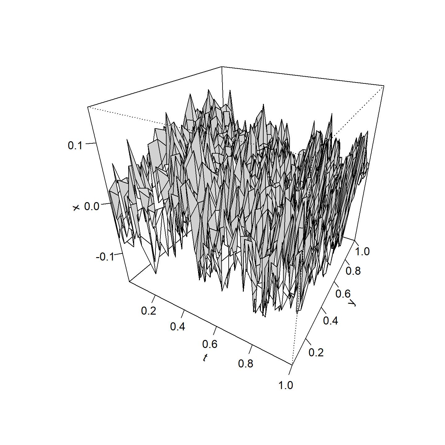
(a) $\theta=$(0,0.1,0.1,0.1)

(b) $\theta=$(0,0.1,0.1,1)

(c) $\theta=$(0,0.1,0.1,10)

Figure 11: Sample paths with $\sigma=0.1$, 1, 10

Figures 14-17 the sample paths, where $\theta_{0}$, $\theta_{2}$ and $\sigma$ are fixed and only $\theta_{1}$ is changed. Figures 14-14 show that the variation of the sample path is large near $y=0$ and small near $y=1$ when $\theta_{1}>0$. This trend increases as the value of $\theta_{1}$ increases.

(a) $\theta=$(0,0.1,0.1,1)

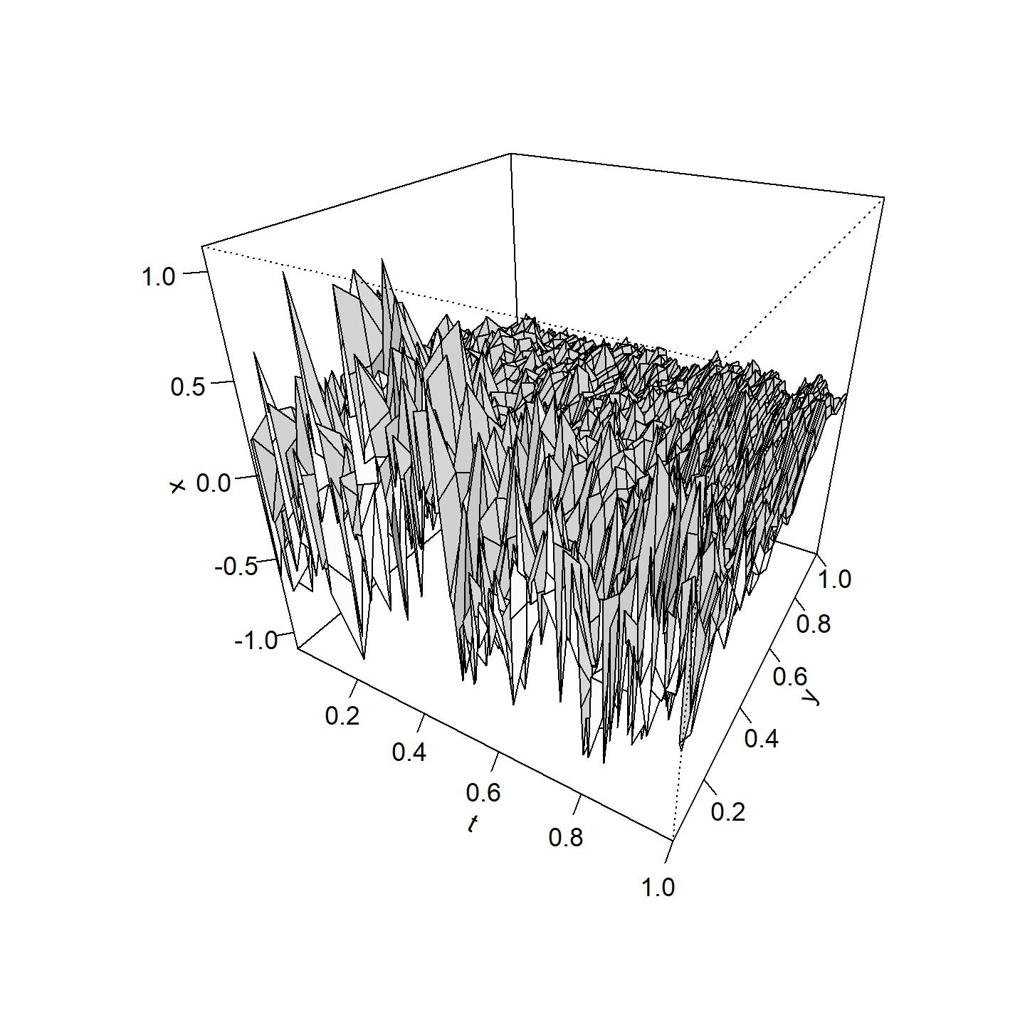
(b) $\theta=$(0,0.5,0.1,1)

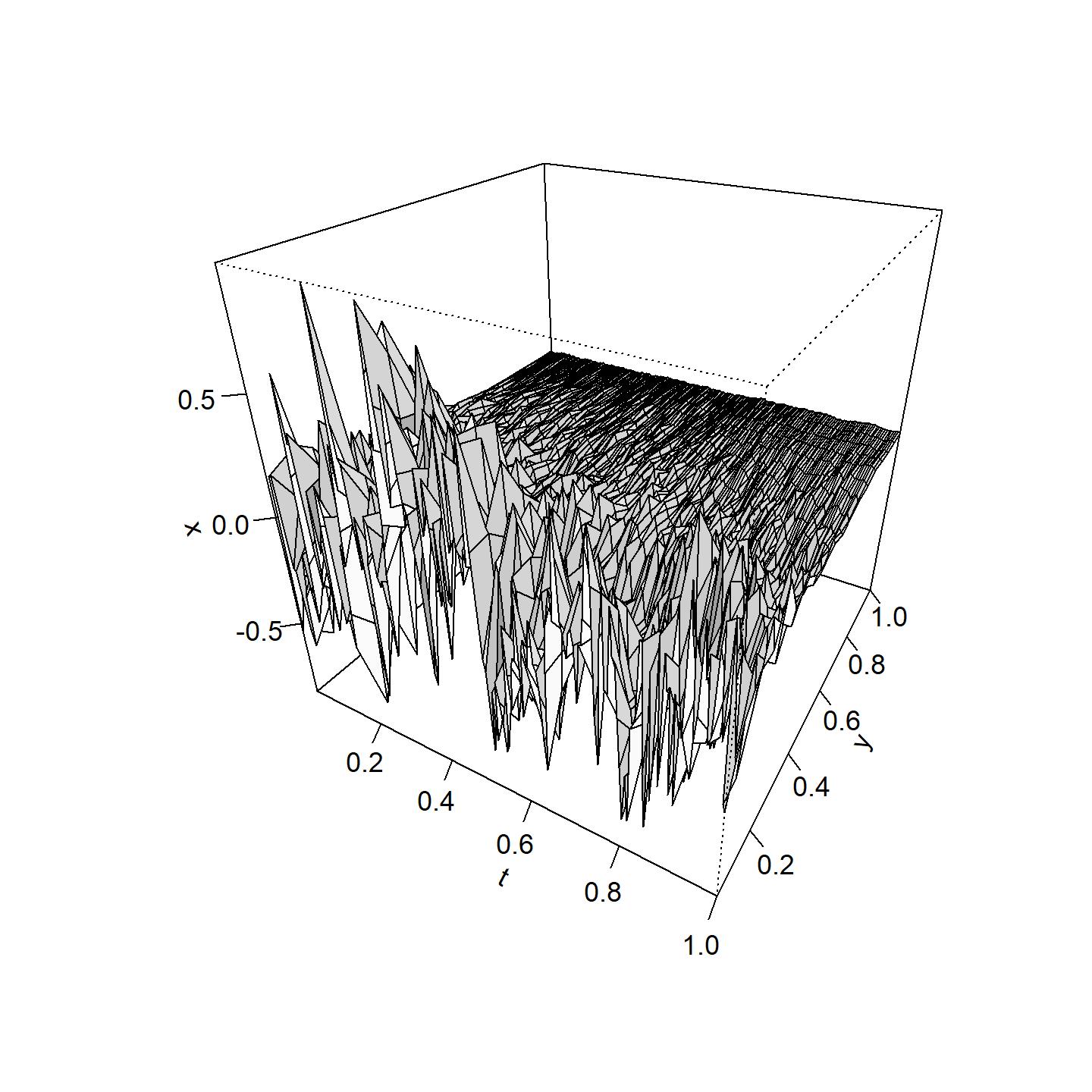
(c) $\theta=$(0,1,0.1,1)

Figure 12: Sample paths with $\theta_{1}=0.1,0.5,1$

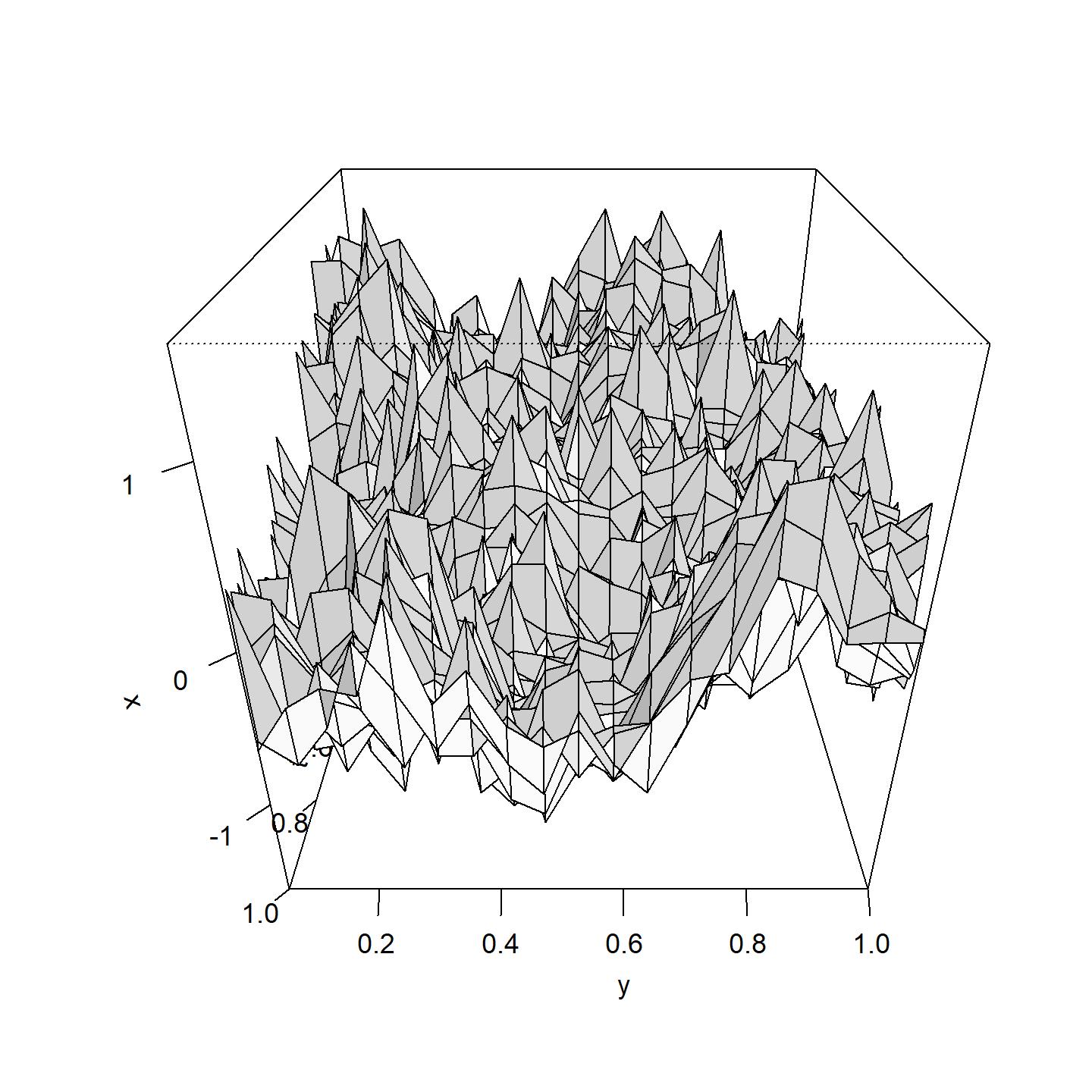
(a) $\theta=$(0,0.1,0.1,1)

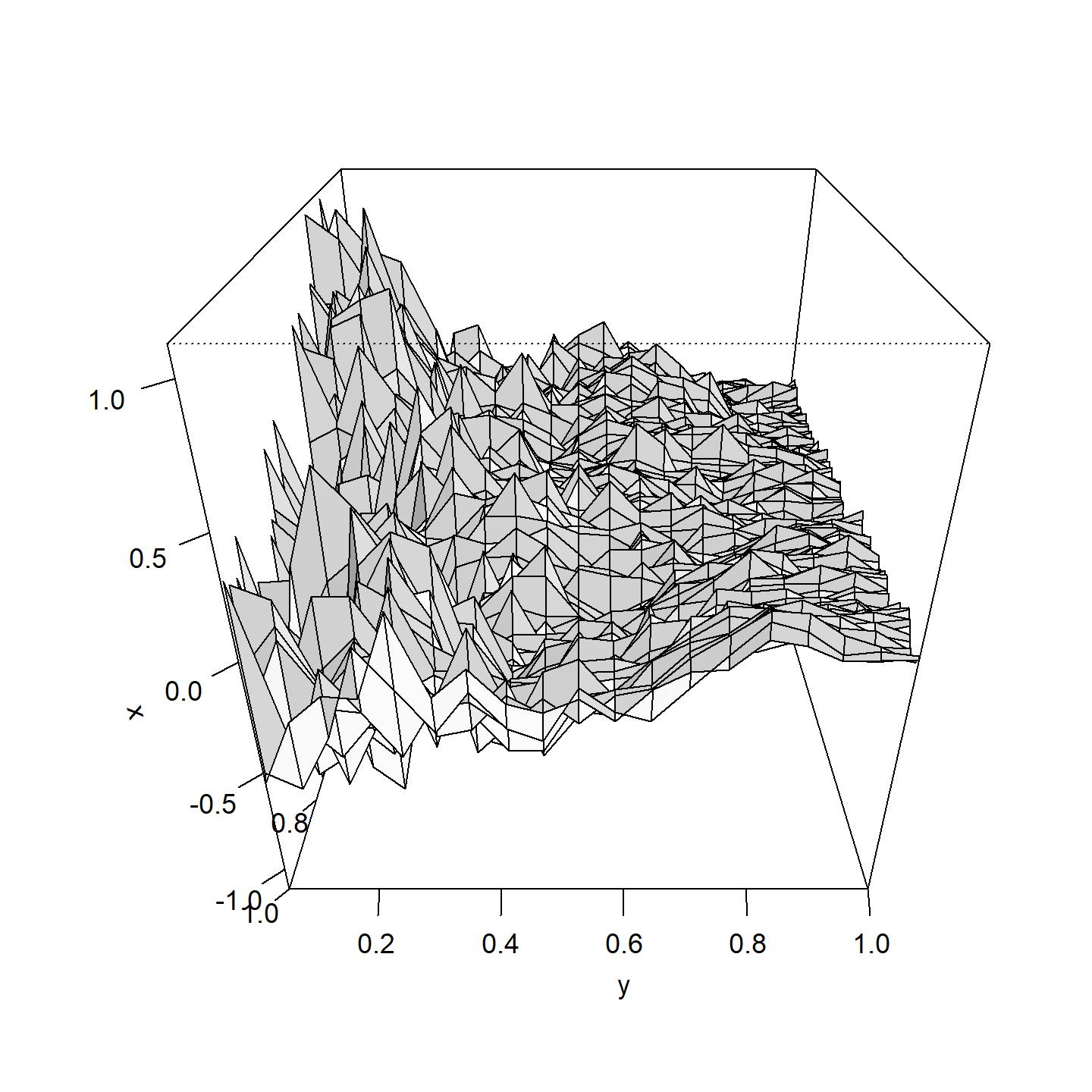
(b) $\theta=$(0,0.5,0.1,1)

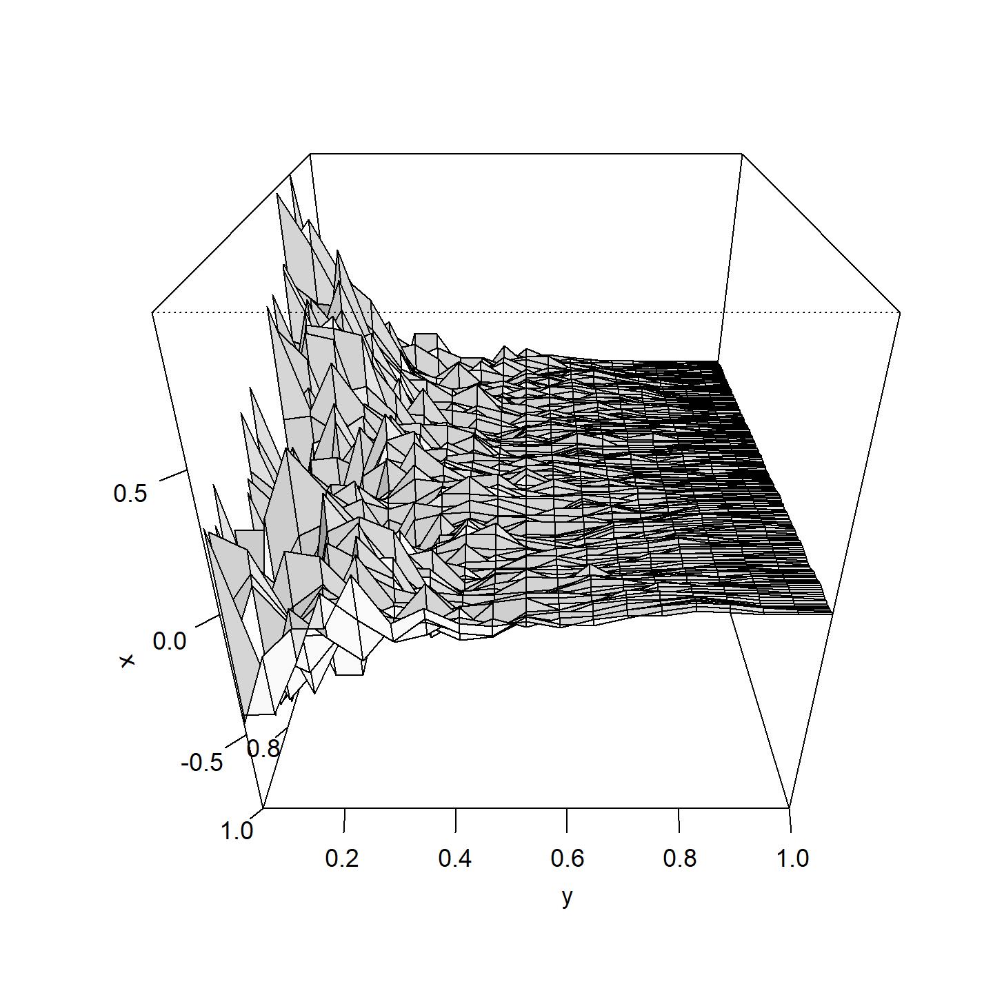
(c) $\theta=$(0,1,0.1,1)

Figure 13: Sample paths with $\theta_{1}=0.1,0.5,1$ (y-axis side)

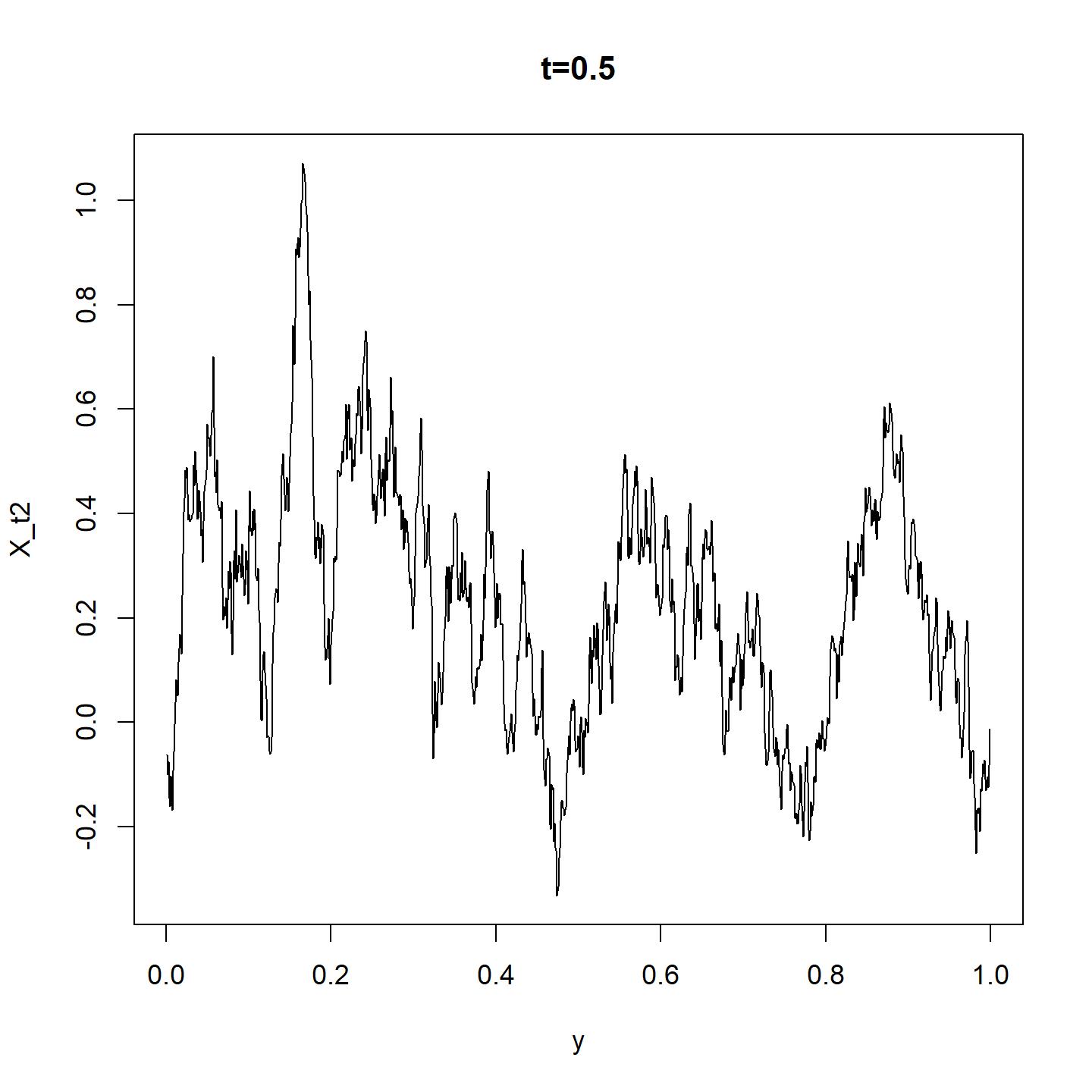
(a) $\theta=$(0,0.1,0.1,1)

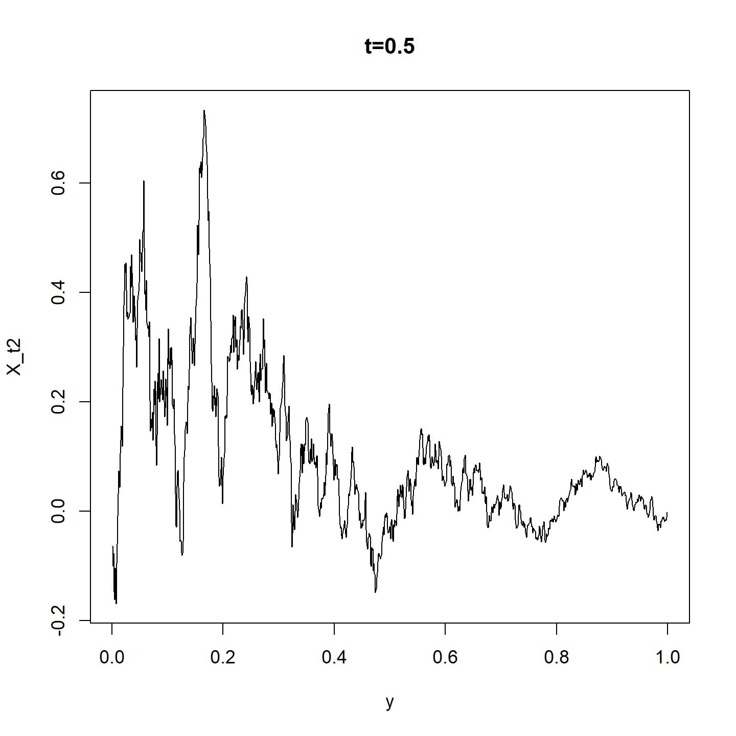
(b) $\theta=$(0,0.5,0.1,1)

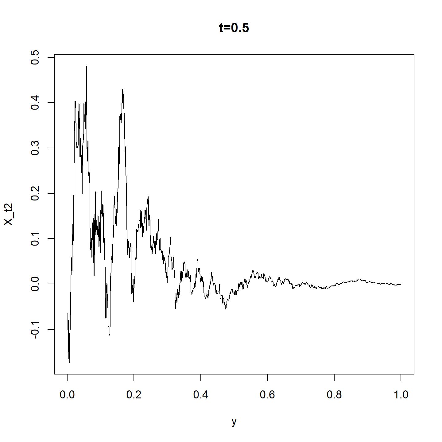
(c) $\theta=$(0,1,0.1,1)

Figure 14: Sample paths with $\theta_{1}=0.1,0.5,1$ (cross section at $t=0.5$)

Figures 17-17 show that the variation of the sample path is small near $y=0$ and large near $y=1$ when $\theta_{1}<0$. This trend increases as the value of $\theta_{1}$ decreases.

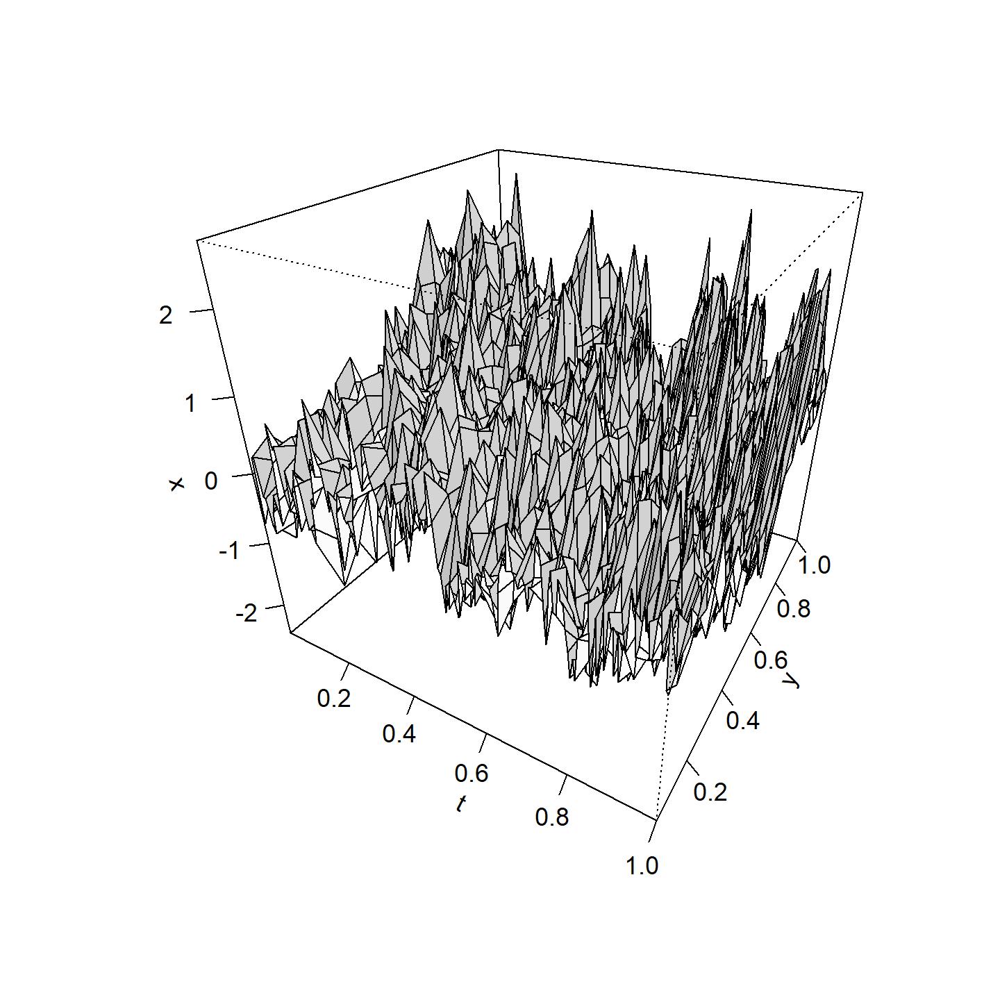
(a) $\theta=$(0,-0.1,0.1,1)

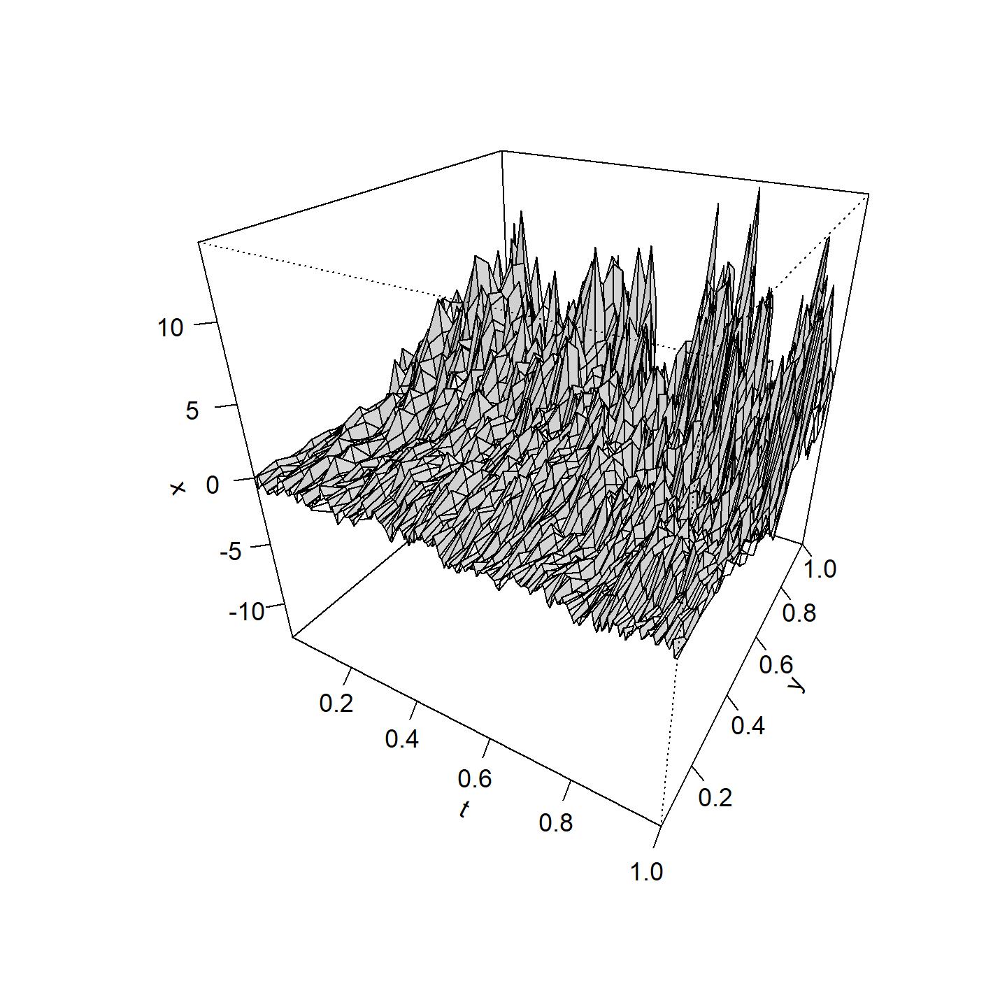
(b) $\theta=$(0,-0.5,0.1,1)

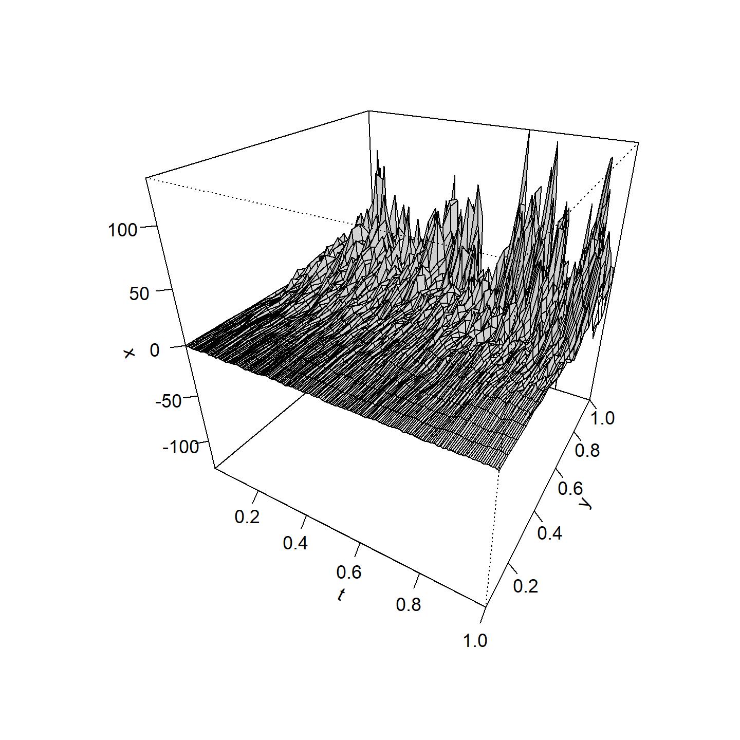
(c) $\theta=$(0,-1,0.1,1)

Figure 15: Sample paths with $\theta_{1}=-0.1,-0.5,-1$

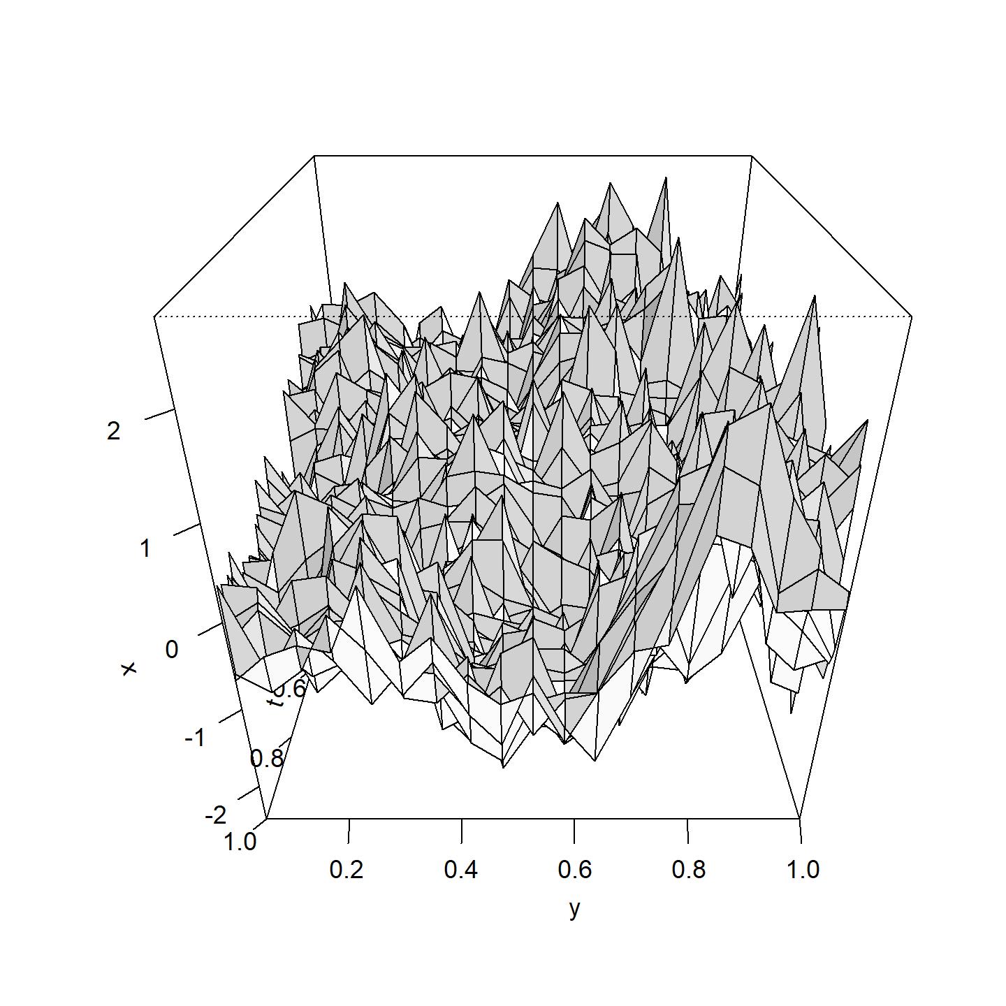
(a) $\theta=$(0,-0.1,0.1,1)

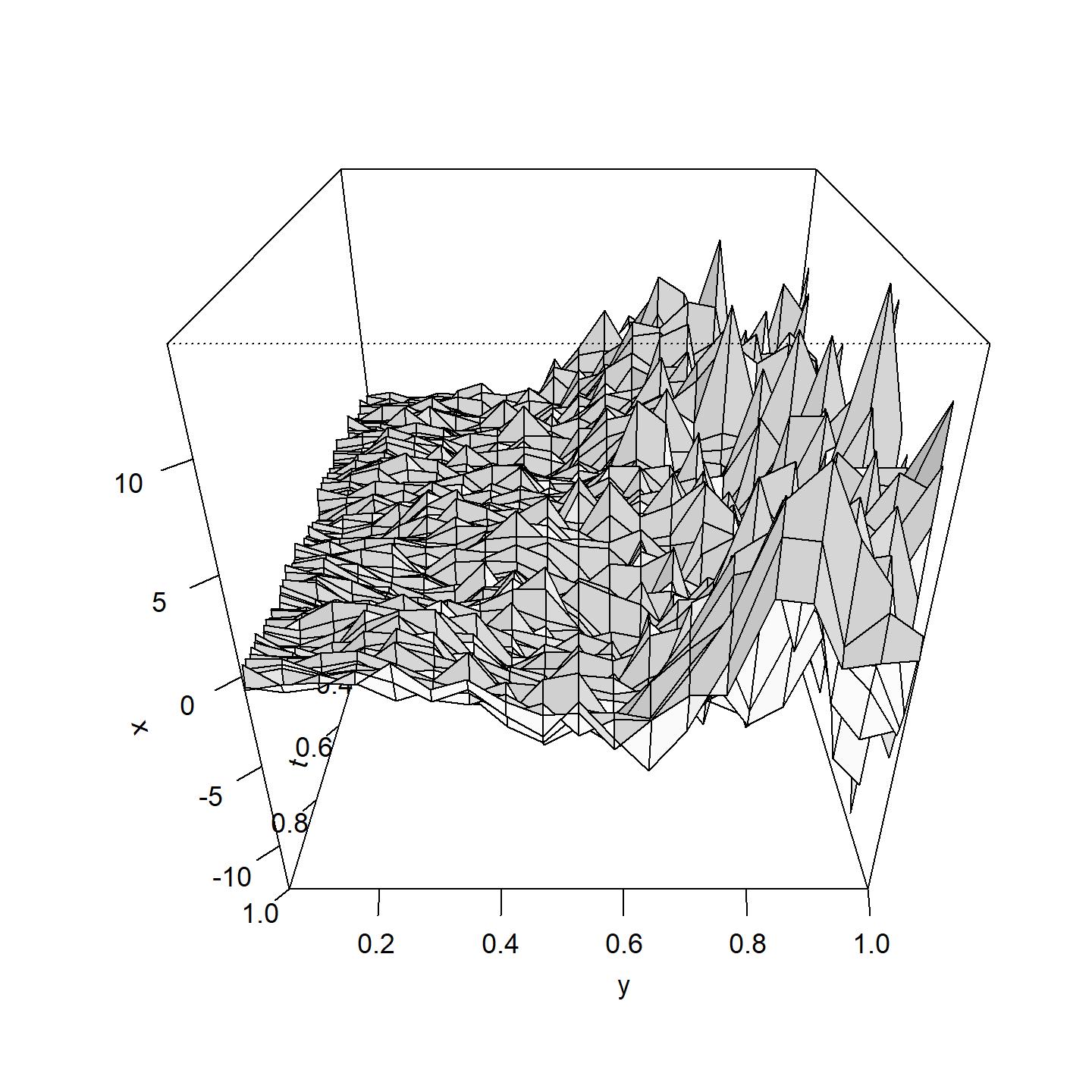
(b) $\theta=$(0,-0.5,0.1,1)

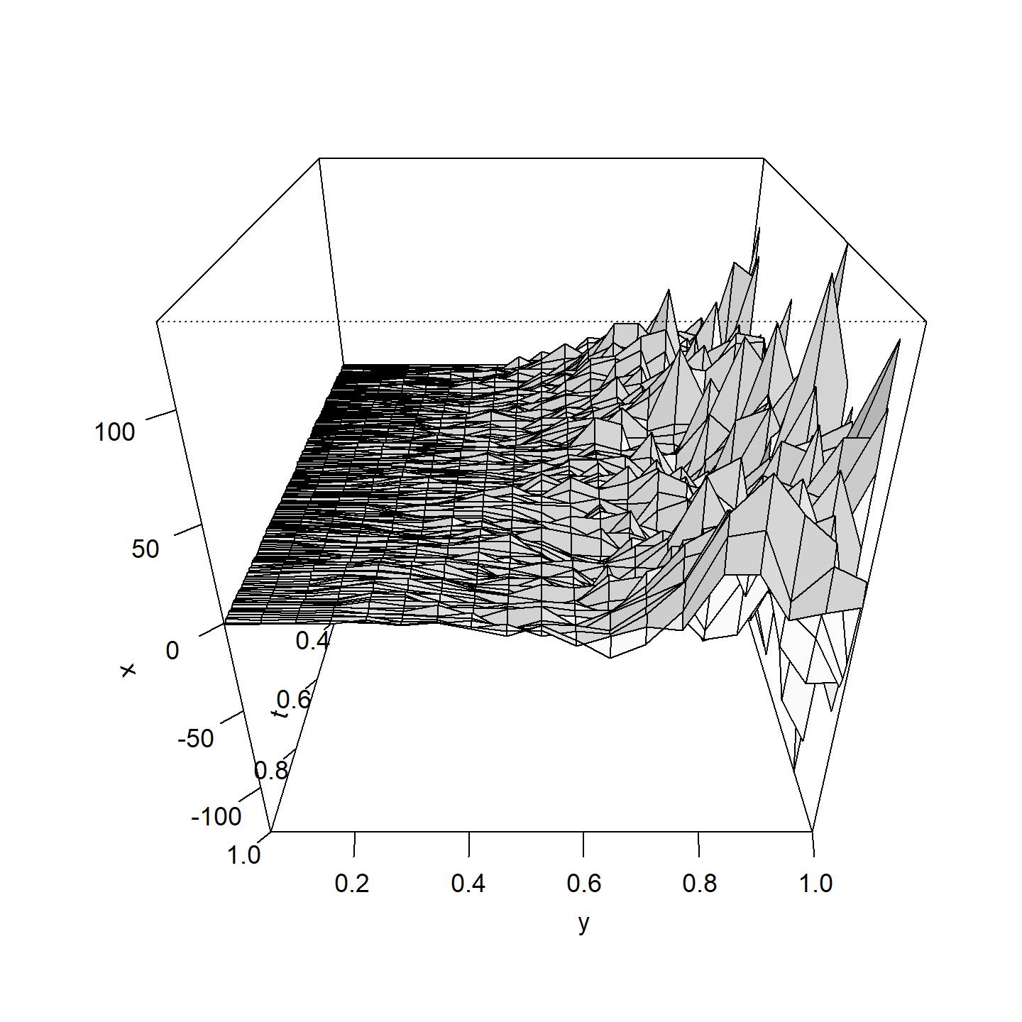
(c) $\theta=$(0,-1,0.1,1)

Figure 16: Sample paths with $\theta_{1}=-0.1,-0.5,-1$ (y-axis side)

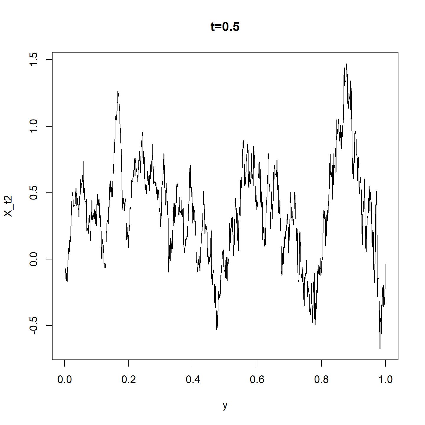
(a) $\theta=$(0,-0.1,0.1,1)

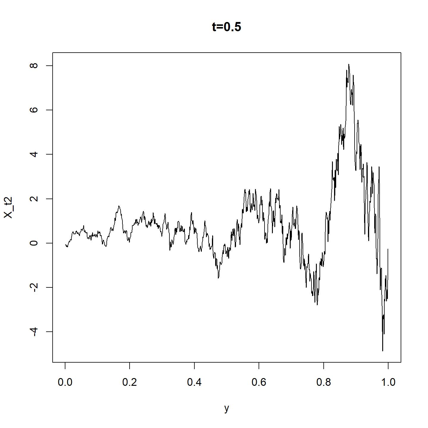
(b) $\theta=$(0,-0.5,0.1,1)

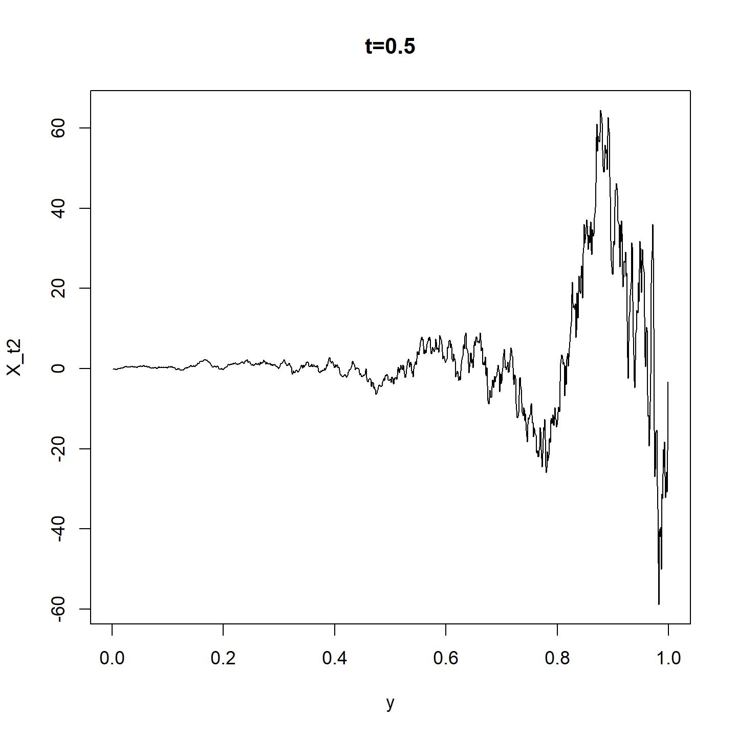
(c) $\theta=$(0,-1,0.1,1)

Figure 17: Sample paths with $\theta_{1}=-0.1,-0.5,-1$ (cross section at $t=0.5$)

Figures 20-20 are the sample paths, where $\theta_{0}$, $\theta_{1}$ and $\sigma$ are fixed and only $\theta_{2}$ is changed. These show that the variation of the sample path is large near $y=0$ and small near $y=1$ and this trend increases as the value of $\theta_{2}$ decreases.

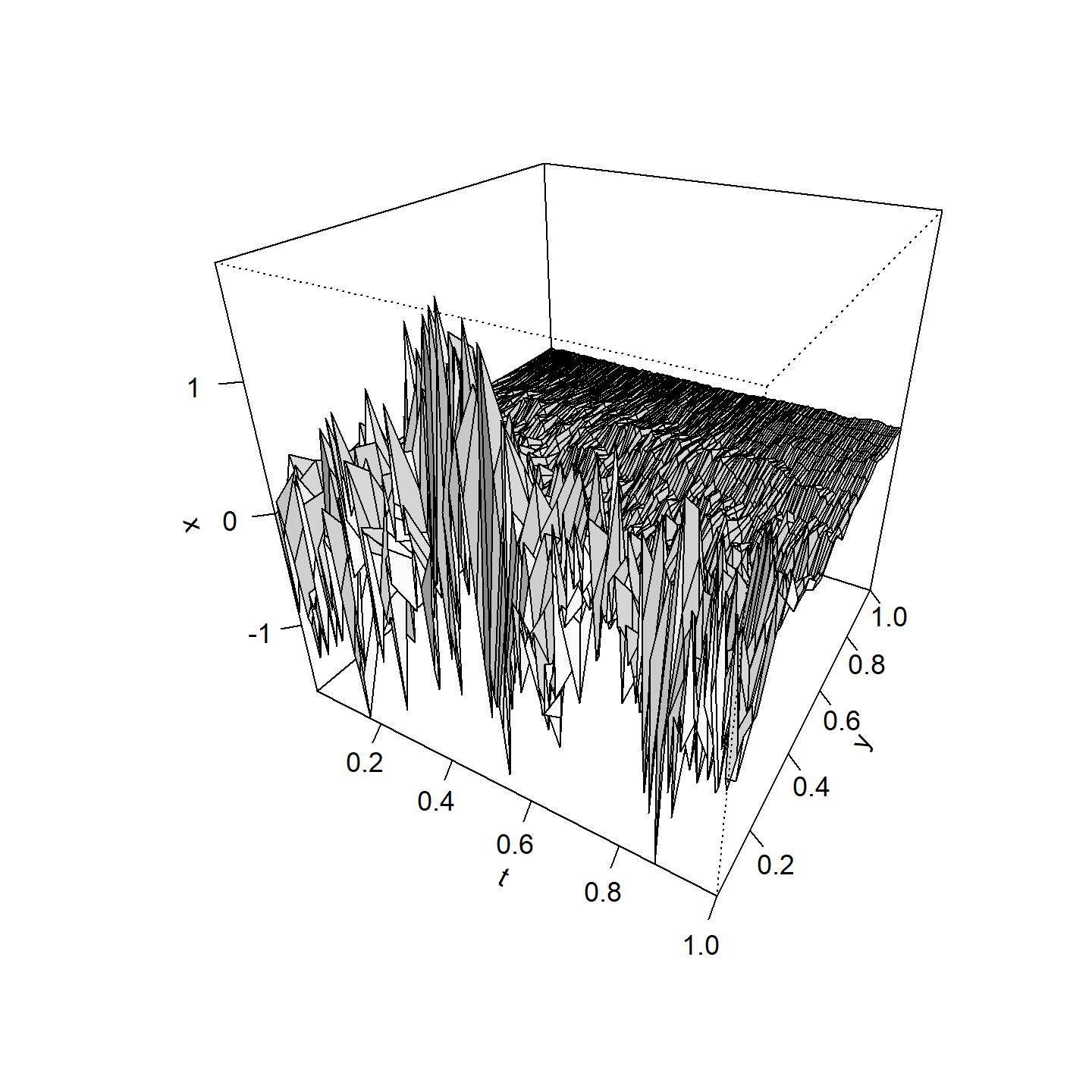
(a) $\theta=$(0,0.1,0.01,1)

(b) $\theta=$(0,0.1,0.1,1)

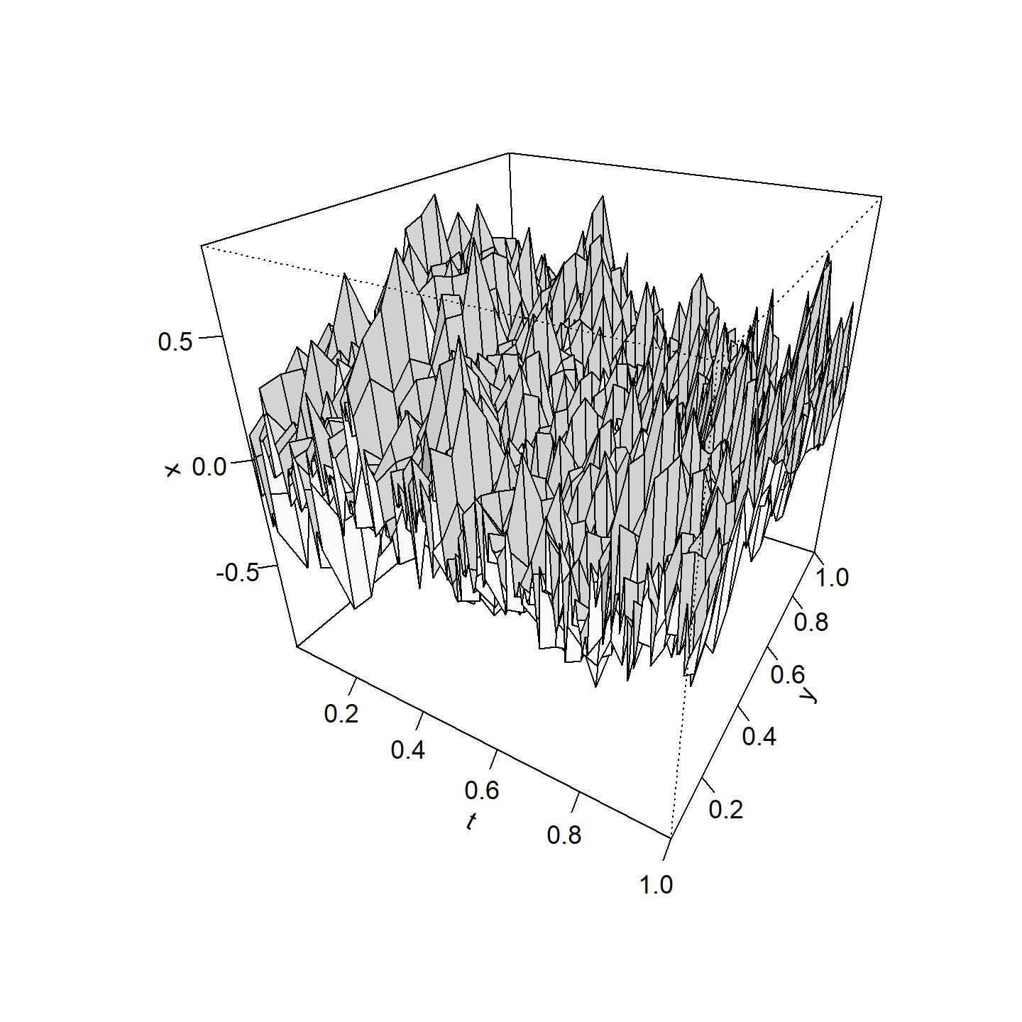
(c) $\theta=$(0,0.1,1,1)

Figure 18: Sample paths with $\theta_{2}=0.01,0.1,1$

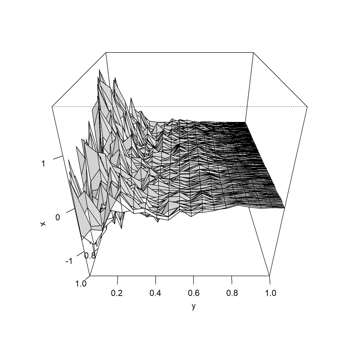
(a) $\theta=$(0,0.1,0.01,1)

(b) $\theta=$(0,0.1,0.1,1)

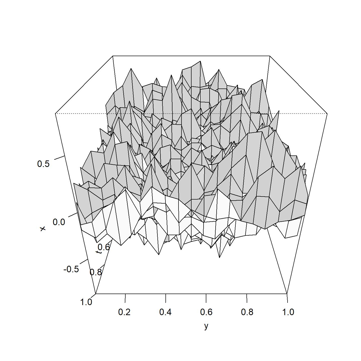
(c) $\theta=$(0,0.1,1,1)

Figure 19: Sample paths with $\theta_{2}=0.01,0.1,1$ (y-axis side)

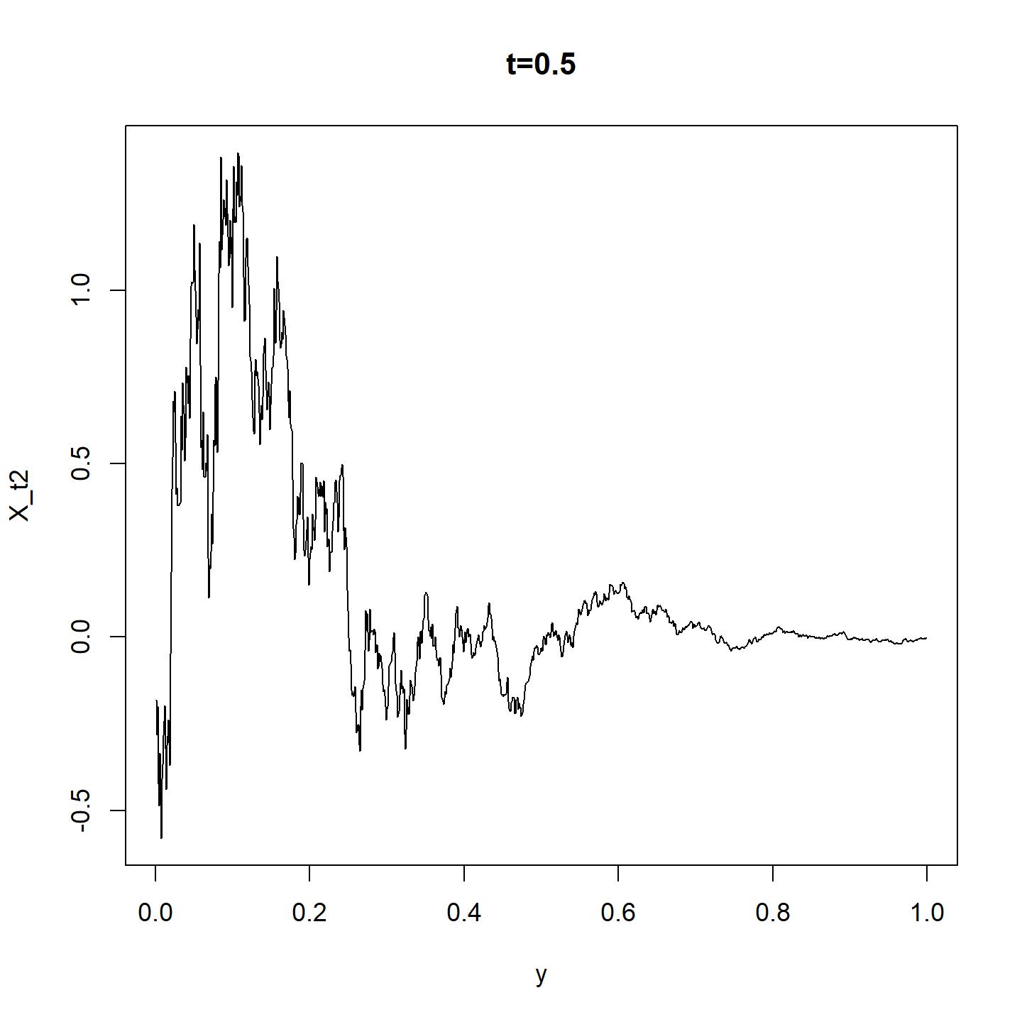
(a) $\theta=$(0,0.1,0.01,1)

(b) $\theta=$(0,0.1,0.1,1)

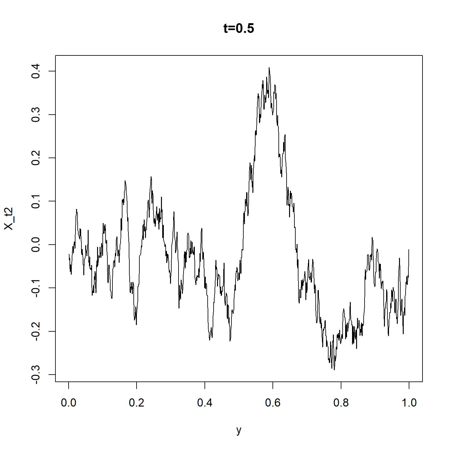
(c) $\theta=$(0,0.1,1,1)

Figure 20: Sample paths with $\theta_{2}=0.01,0.1,1$ (cross section at $t=0.5$)

Figures 23-26 are the sample paths, where $\theta_{1}$, $\theta_{2}$ and $\sigma$ are fixed and only $\theta_{0}$ is changed. Figures 23-23 show the sample paths with $T=1$ and Figures 24-26 show the sample paths with $T=100$. $\theta_{0}$ affects the shape of the sample path when $y$ is fixed and $t$ is changed. When $T$ is large, the effect of $\theta_{0}$ is large.

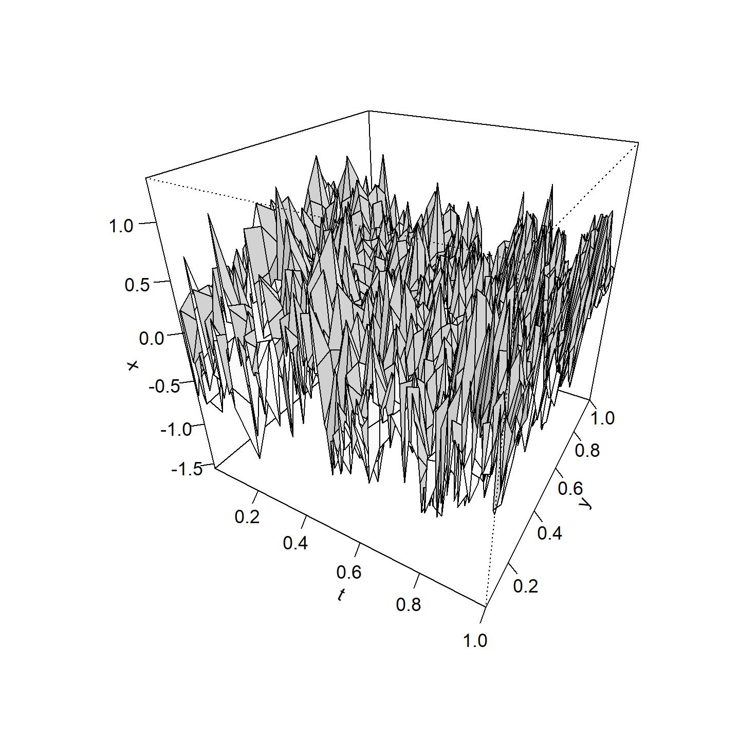
(a) $\theta=$(-5,0.1,0.1,1)

(b) $\theta=$(0,0.1,0.1,1)

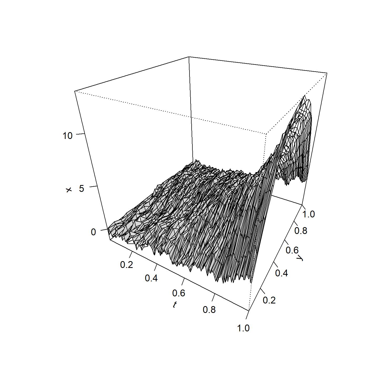
(c) $\theta=$(5,0.1,0.1,1)

Figure 21: Sample paths with $\theta_{0}=-5,0,5$ and $T=1$

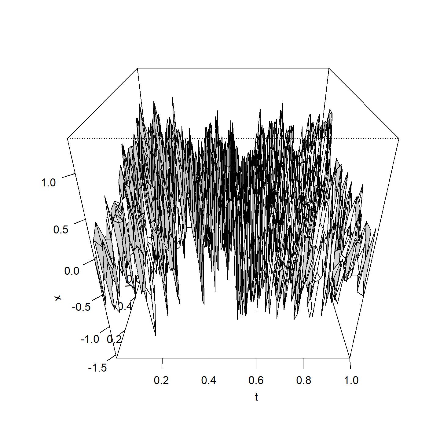
(a) $\theta=$(-5,0.1,0.1,1)

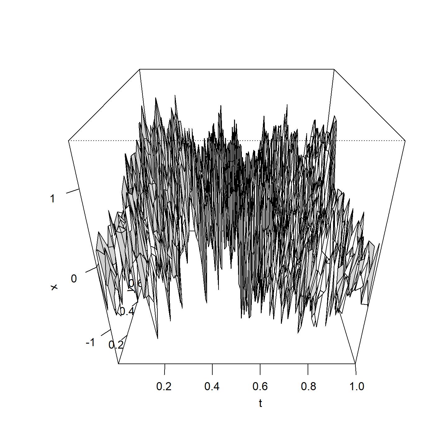
(b) $\theta=$(0,0.1,0.1,1)

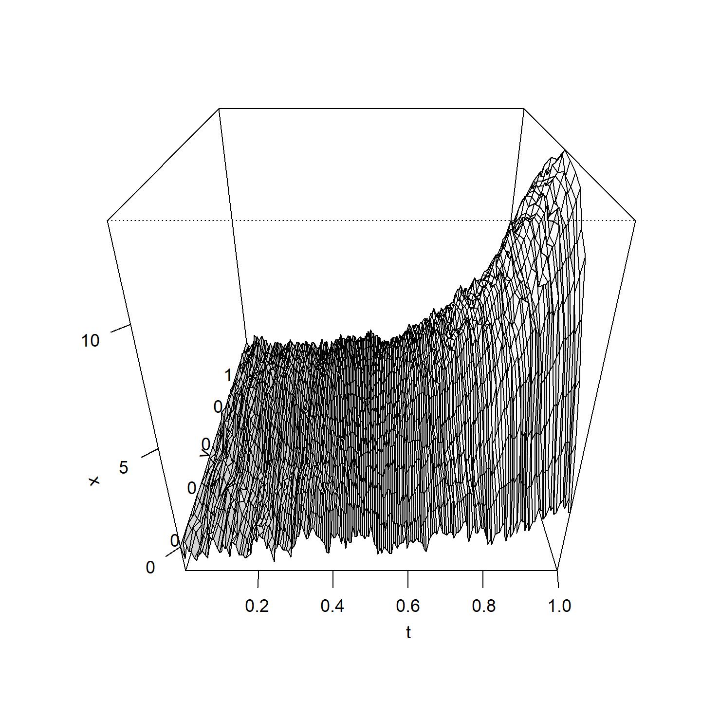
(c) $\theta=$(5,0.1,0.1,1)

Figure 22: Sample paths with $\theta_{0}=-5,0,5$ and $T=1$ (t-axis side)

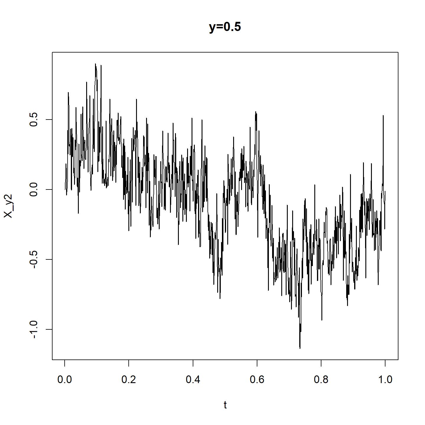
(a) $\theta=$(-5,0.1,0.1,1)

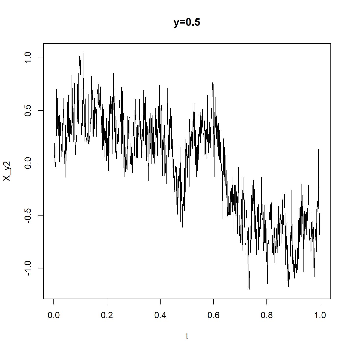
(b) $\theta=$(0,0.1,0.1,1)

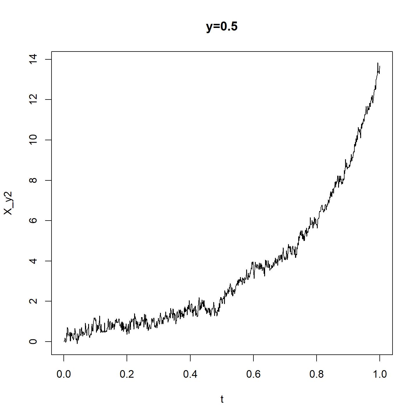
(c) $\theta=$(5,0.1,0.1,1)

Figure 23: Sample paths with $\theta_{0}=-5,0,5$ and $T=100$ (cross section at $y=0.5$)

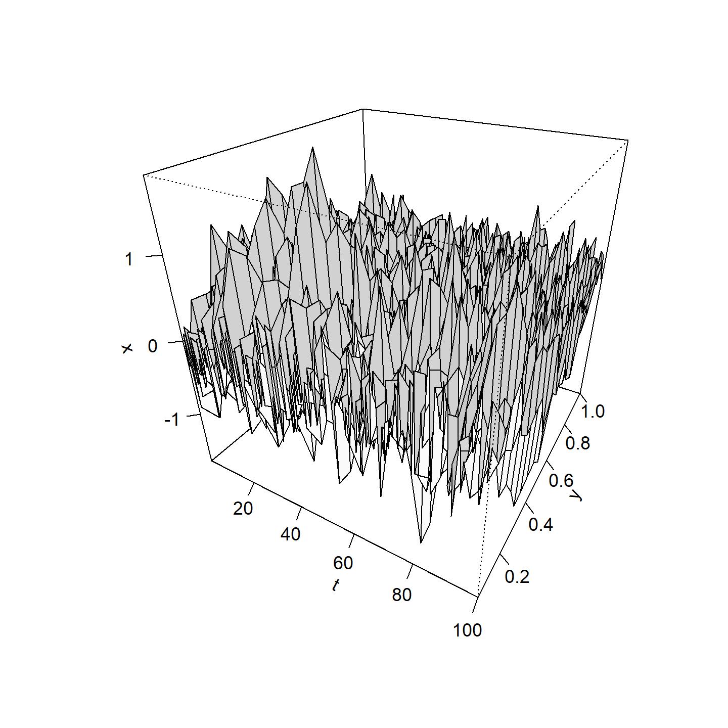
(a) $\theta=$(-5,0.1,0.1,1)

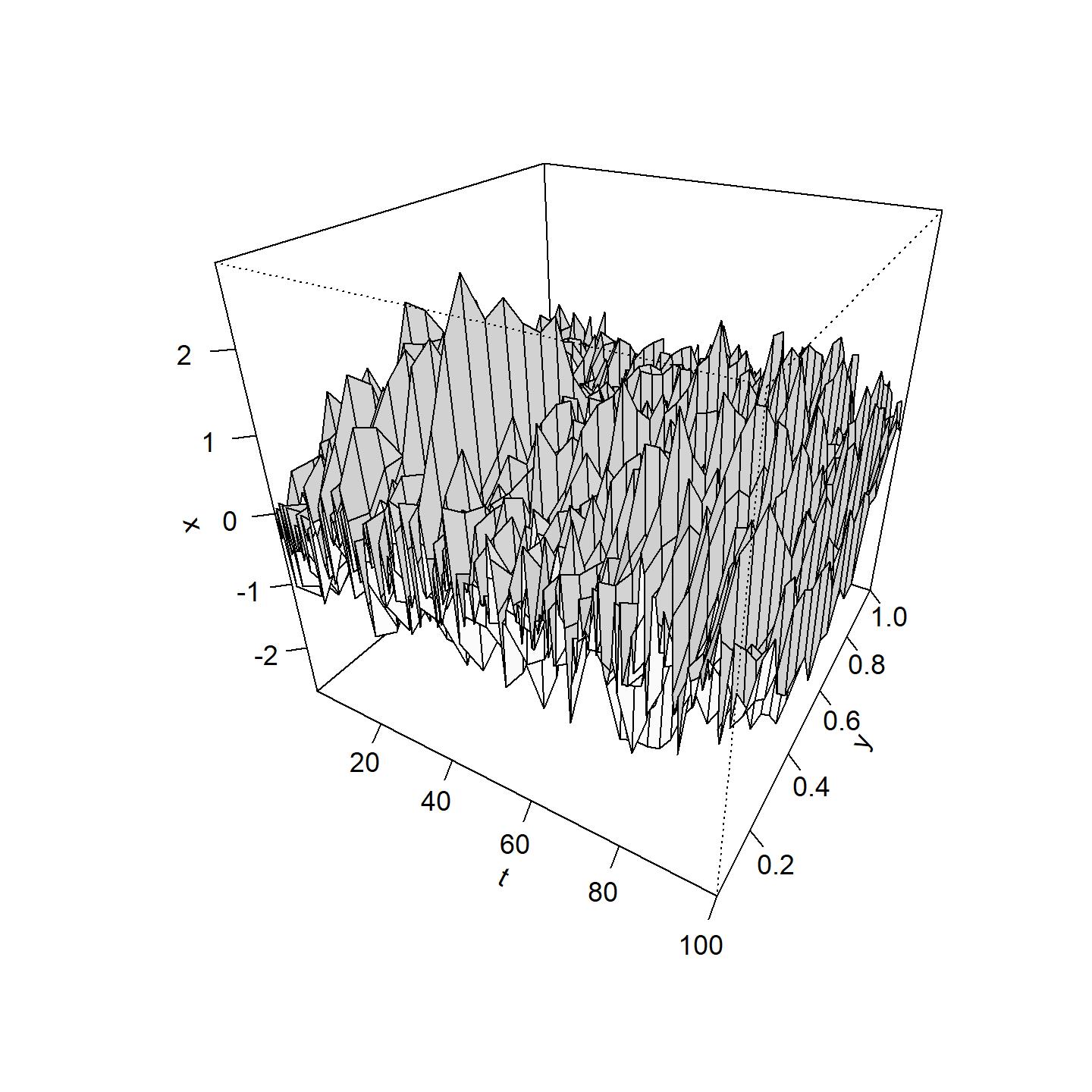
(b) $\theta=$(0,0.1,0.1,1)

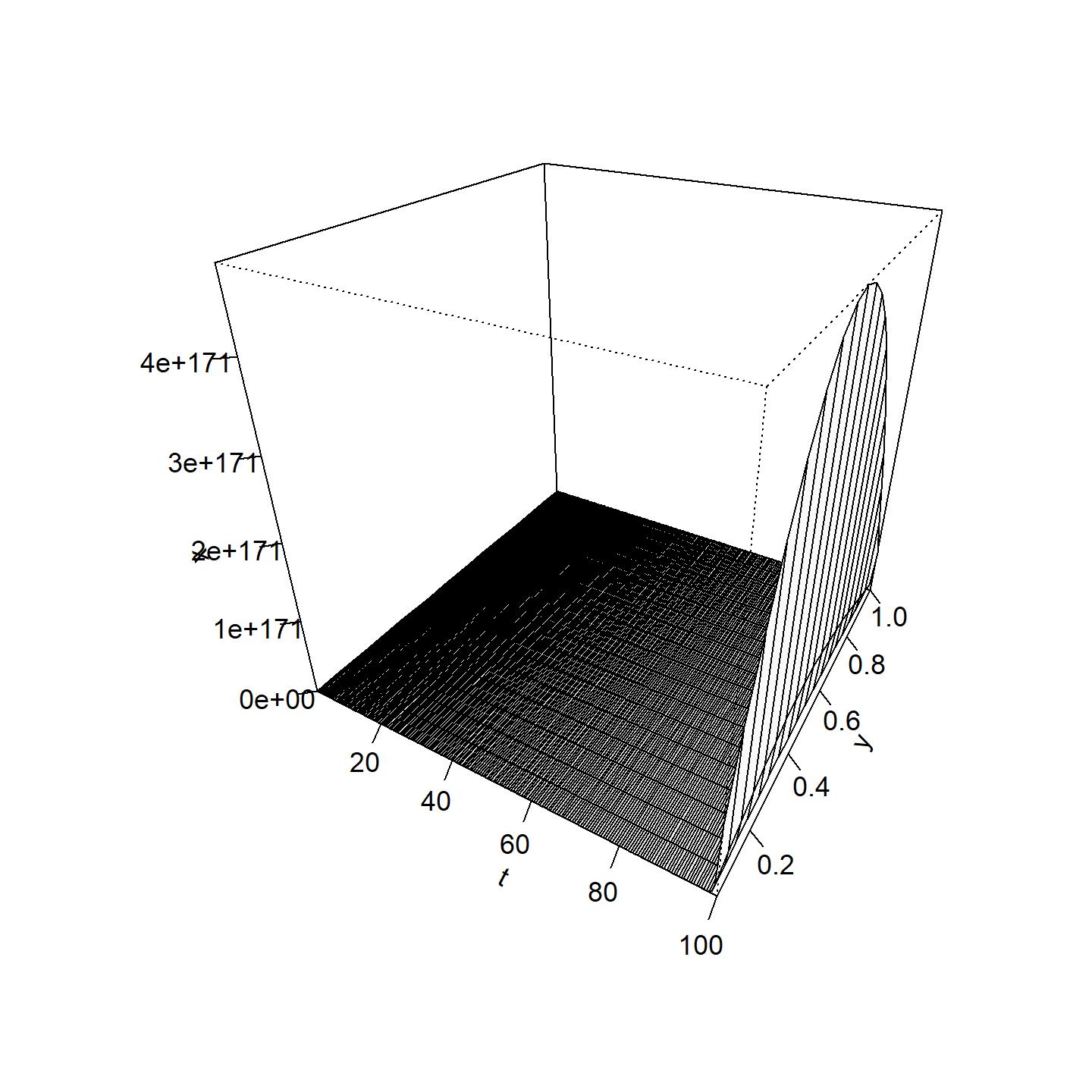
(c) $\theta=$(5,0.1,0.1,1)

Figure 24: Sample paths with $\theta_{0}=-5,0,5$ and $T=100$

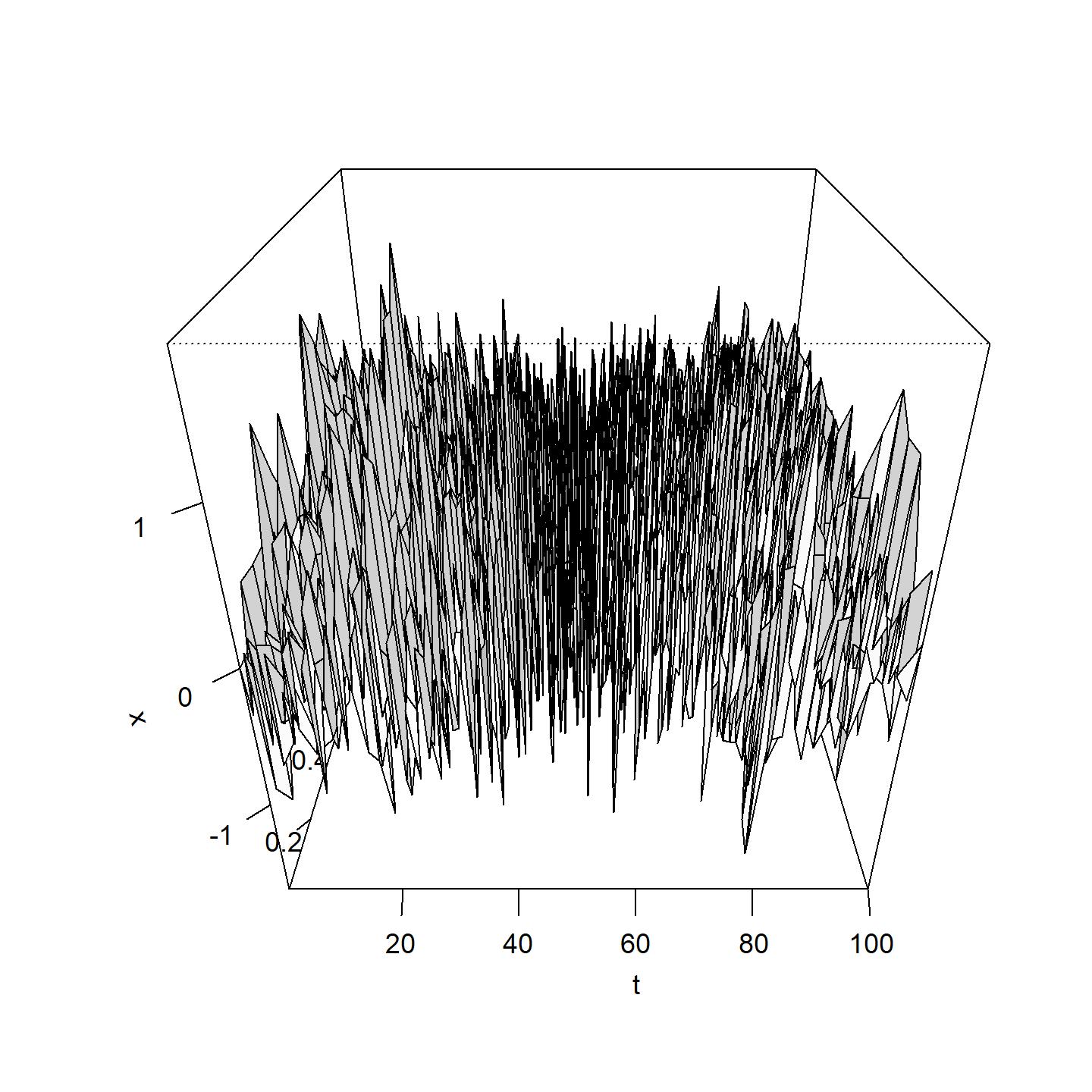
(a) $\theta=$(-5,0.1,0.1,1)

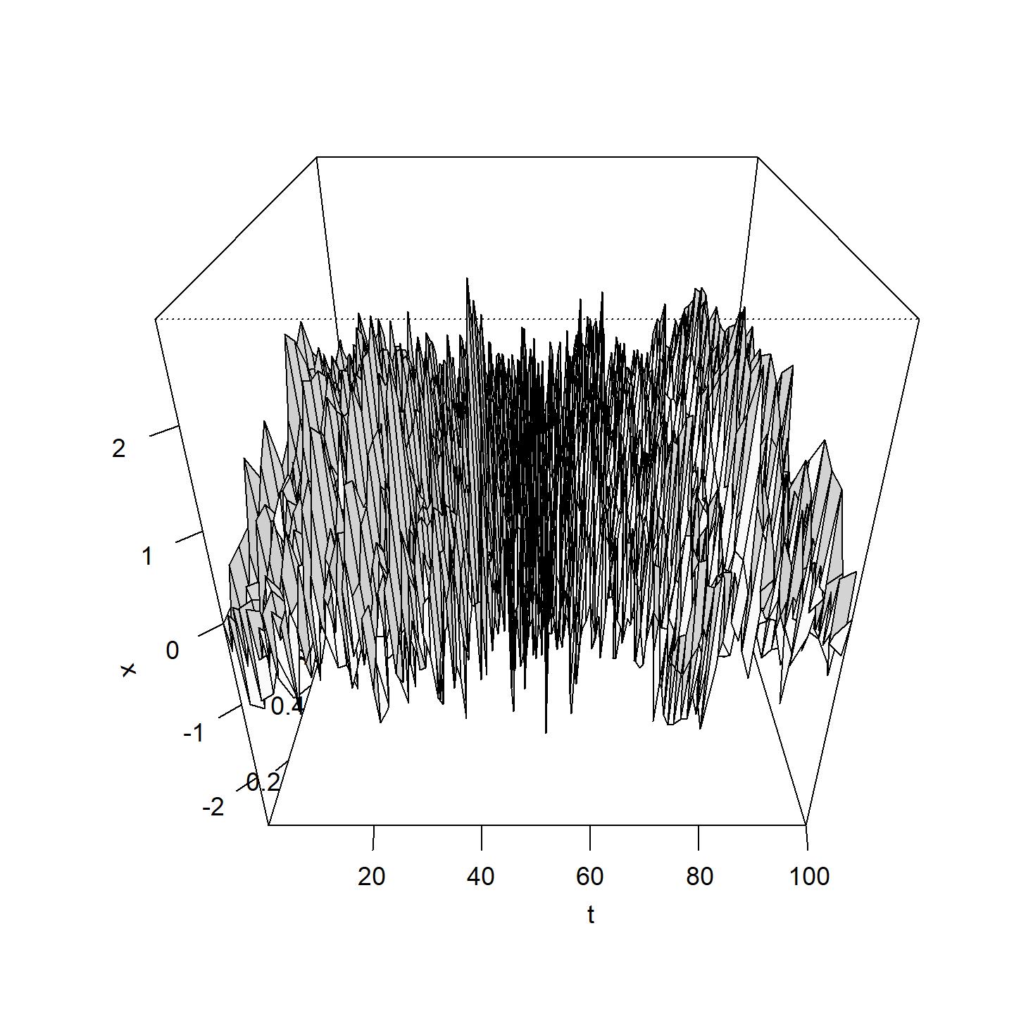
(b) $\theta=$(0,0.1,0.1,1)

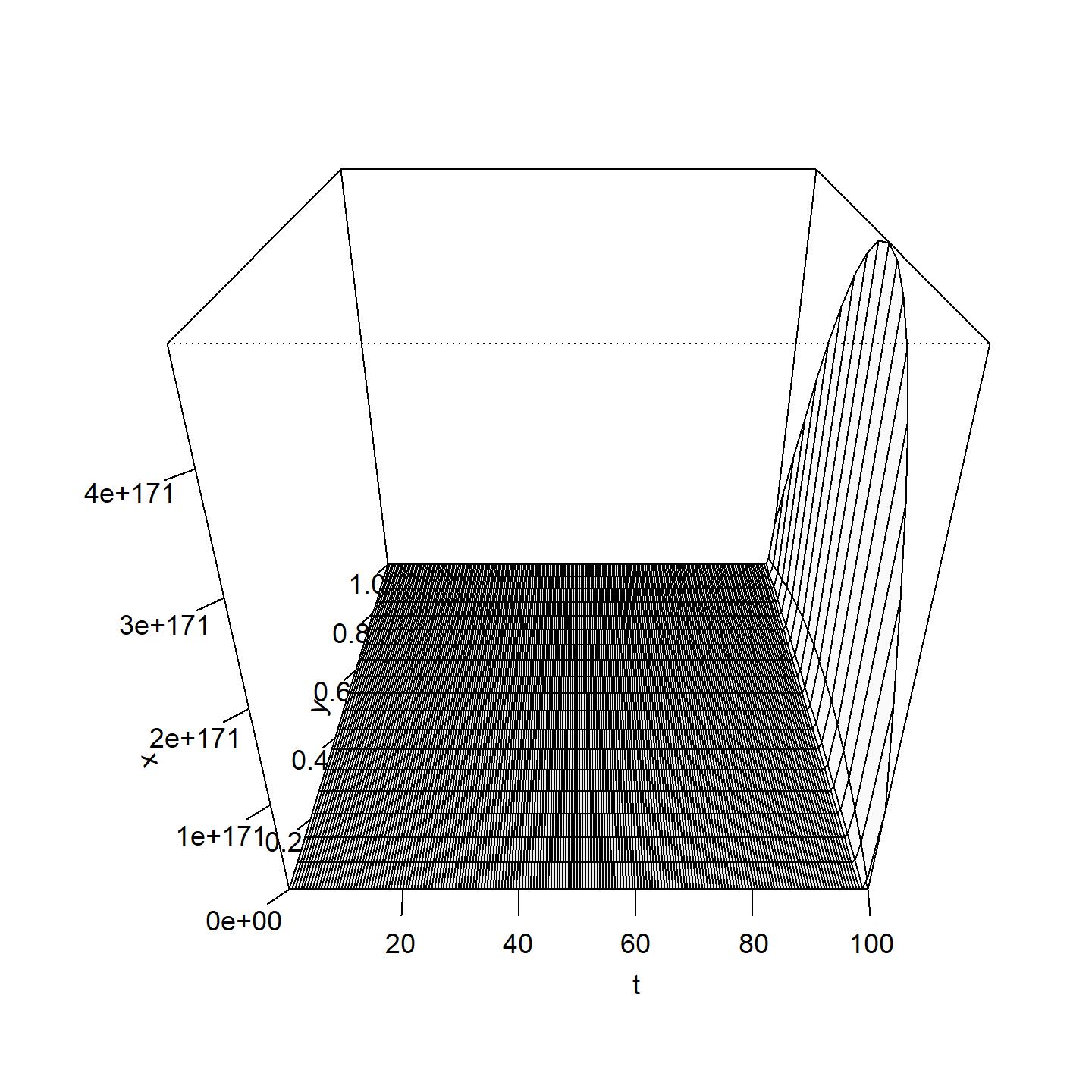
(c) $\theta=$(5,0.1,0.1,1)

Figure 25: Sample paths with $\theta_{0}=-5,0,5$ and $T=100$ (t-axis side)

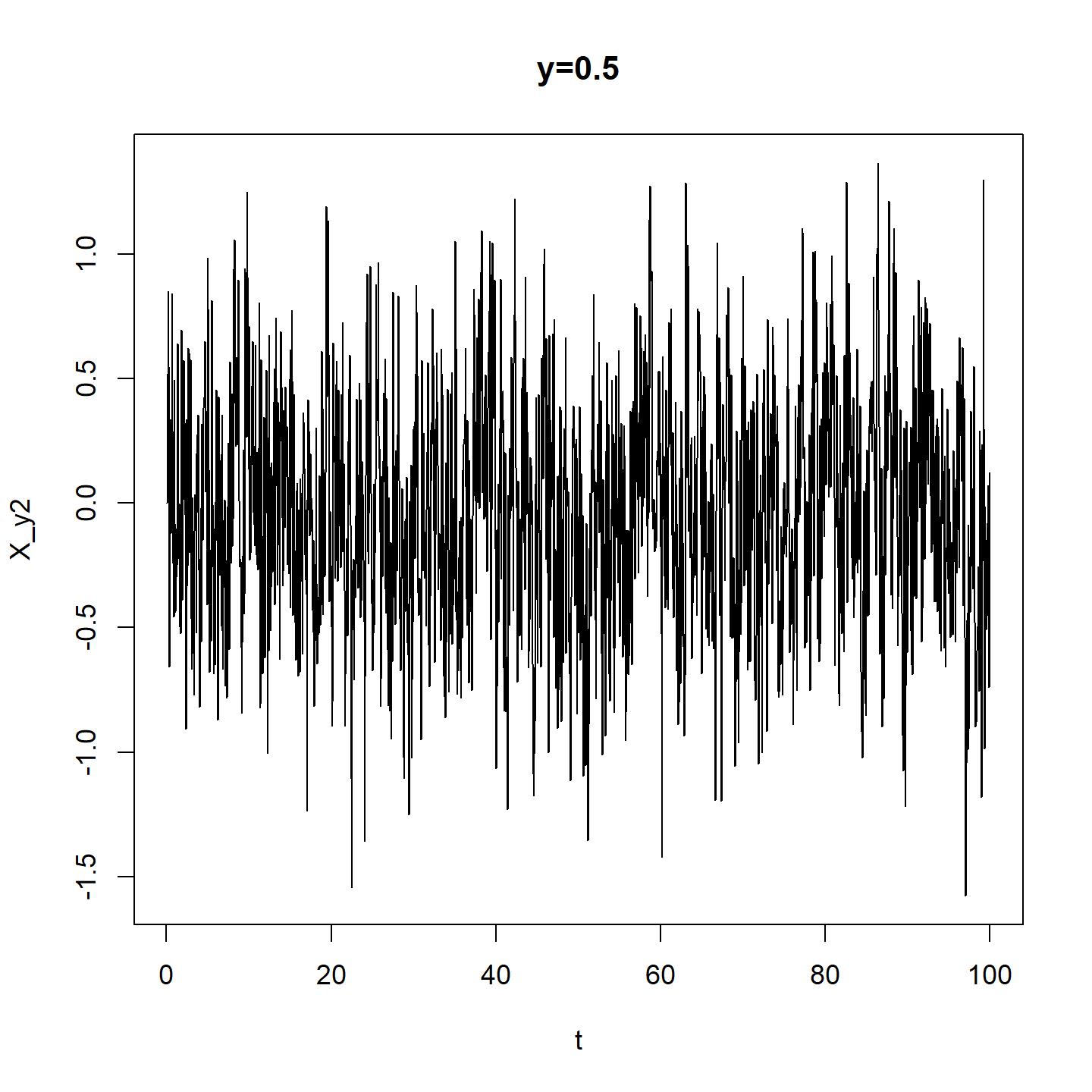
(a) $\theta=$(-5,0.1,0.1,1)

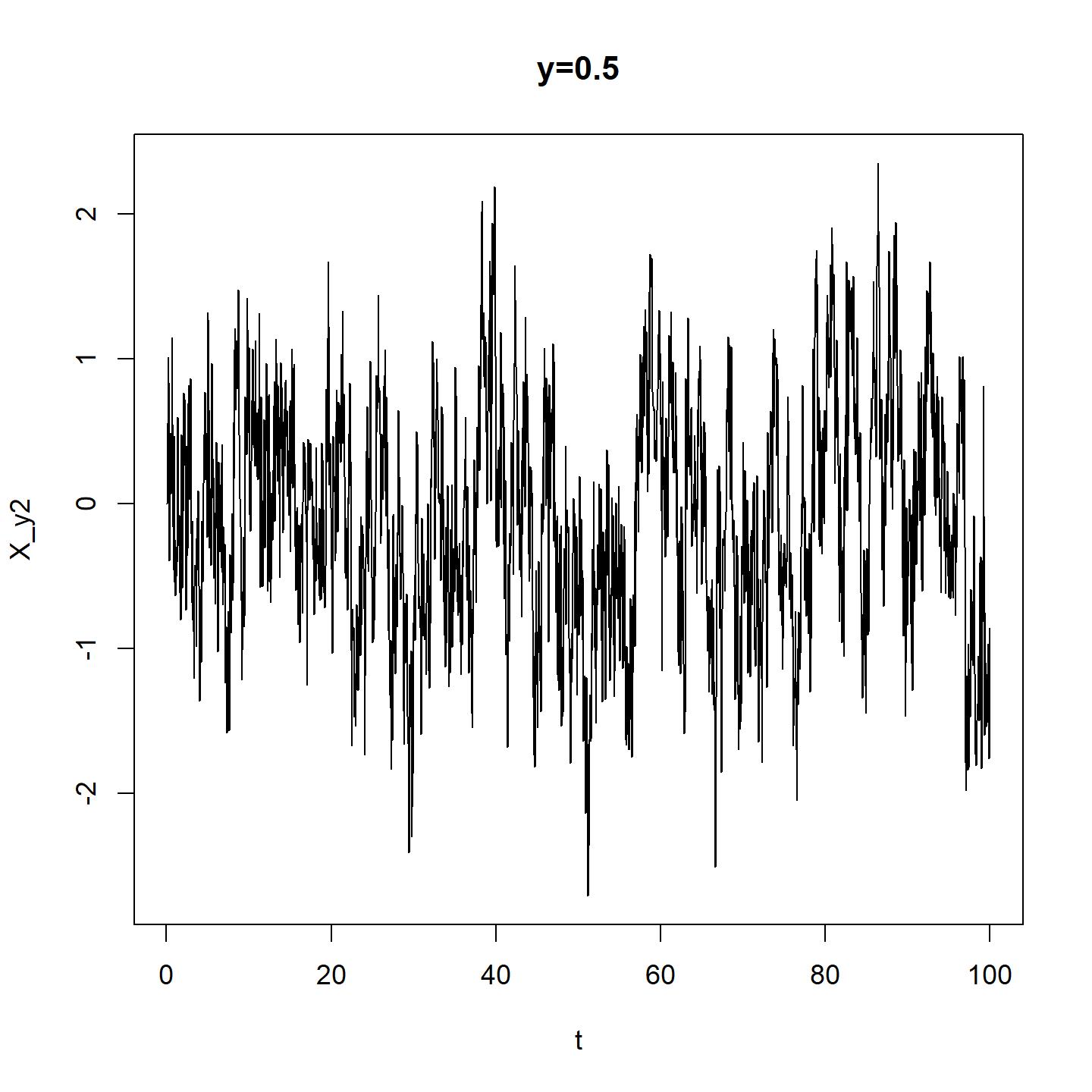
(b) $\theta=$(0,0.1,0.1,1)

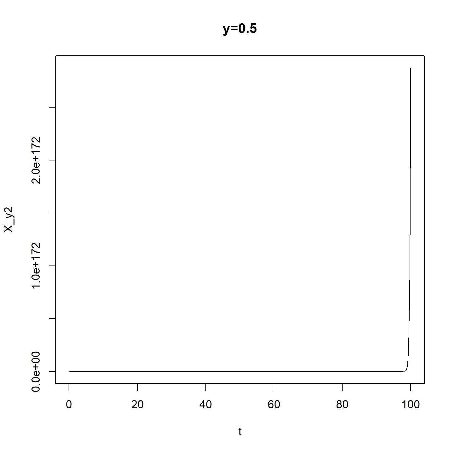
(c) $\theta=$(5,0.1,0.1,1)

Figure 26: Sample paths with $\theta_{0}=-5,0,5$ and $T=100$ (cross section at $y=0.5$)

References

Bibby, B. M. and Sørensen, M. (1995). Martingale estimating functions for discretely observed diffusion processes. Bernoulli, 1, 17–39.

Bibinger, M. and Trabs, M. (2017). Volatility estimation for stochastic pdes using high-frequency observations. arXiv:1710.03519.

Chong, C. (2019). High-frequency analysis of parabolic stochastic PDEs. Forthcoming in The Annals of Statistics.

Cialenco, I. (2018). Statistical inference for SPDEs: an overview. Statistical Inference for Stochastic Processes, 21, 309–329.

Cialenco, I., Delgado-Vences, F. and Kim, H.-J. (2019). Drift Estimation for Discretely Sampled SPDEs. arXiv:1904.10884.

Cialenco, I. and Glatt-Holtz, N. (2011). Parameter estimation for the stochastically perturbed Navier-Stokes equations. Stochastic Processes and their Applications.  121, 701–724.

Cialenco, I., Gong, R. and Y. Huang, Y. (2018). Trajectory fitting estimators for SPDEs driven by additive noise. Statistical Inference for Stochastic Processes.  21, 1–19.

Cialenco, I. and Huang, Y. (2017). A note on parameter estimation for discretely sampled SPDEs. arXiv:1710.01649.

Cont, R. (2005). Modeling term structure dynamics: an infinite dimensional approach. International Journal of Theoretical and Applied Finance, 8, 357–380.

De Gregorio, A. and Iacus, S. M. (2013). On a family of test statistics for discretely observed diffusion processes. Journal of Multivariate Analysis, 122, 292–316.

Dohnal, G. (1987). On Estimating the Diffusion Coefficient. Journal of Applied Probability, 24, 105–114.

Florens-Zmirou, D. (1989). Approximate discrete time schemes for statistics of diffusion processes. Statistics, 20, 547–557.

Genon-Catalot, V. and Jacod, J. (1993). On the estimation of the diffusion coefficient for multidimensional diffusion processes. Annales de l’Institut Henri Poincaré Probabilités et Statistiques, 29, 119–151.

Genon-Catalot, V.  and Jacod, J. (1994). Estimation of the Diffusion Coefficient for Diffusion Processes: Random Sampling. Scandinavian Journal of Statistics, 21, 193–221.

Kaino, Y. and Uchida, M. (2018). Hybrid estimators for stochastic differential equations from reduced data. Statistical Inference for Stochastic Processes, 21, 435–454.

Kamatani, K. and Uchida, M. (2015). Hybrid multi-step estimators for stochastic differential equations based on sampled data. Statistical Inference for Stochastic Processes, 18, 177–204.

Kessler, M. (1995). Estimation des paramètres d’une diffusion par des contrastes corrigés. Comptes Rendus de l’Académie des Sciences - Series I - Mathematics, 320, 359–362.

Kessler, M. (1997). Estimation of an ergodic diffusion from discrete observations. Scandinavian Journal of Statistics, 24, 211–229.

Kutoyants, Yu. A. (1984). Parameter estimation for stochastic processes. Prakasa Rao, B.L.S. (ed. ) Heldermann, Berlin.

Kutoyants, Yu. A. (2004). Statistical inference for ergodic diffusion processes.  Springer-Verlag, London.

Markussen, B. (2003). Likelihood inference for a discretely observed stochastic partial differential equation. Bernoulli, 9, 745–762.

Masuda, H. (2013a). Asymptotics for functionals of self-normalized residuals of discretely observed stochastic processes. Stochastic Processes and their Applications, 123, 2752–2778.

Masuda, H. (2013b). Convergence of Gaussian quasi-likelihood random fields for ergodic Levy driven SDE observed at high frequency. The Annals of Statistics, 41, 1593–1641.

Nakakita, S. H. and Uchida, M. (2019). Inference for ergodic diffusions plus noise. Scandinavian Journal of Statistics, 46, 470–516.

Ogihara, T.  (2018). Parametric inference for nonsynchronously observed diffusion processes in the presence of market microstructure noise. Bernoulli, 24, 3318–3383.

Ogihara, T. and Yoshida, N. (2011). Quasi-likelihood analysis for the stochastic differential equation with jumps. Statistical Inference for Stochastic Processes, 14, 189–229.

Ogihara, T. and Yoshida, N. (2014). Quasi-likelihood analysis for nonsynchronously observed diffusion processes. Stochastic Processes and their Applications, 124, 2954–3008.

Prakasa Rao, B. L. S. (1983). Asymptotic theory for nonlinear least squares estimator for diffusion processes. Math. Operationsforsch. Statist. Ser. Statist., 14, 195–209.

Prakasa Rao, B. L. S. (1988). Statistical inference from sampled data for stochastic processes. Contemporary Mathematics, 80, 249–284. Amer. Math. Soc., Providence, RI.

Shimizu, Y. (2006). M-estimation for discretely observed ergodic diffusion processes with infinitely many jumps. Statistical Inference for Stochastic Processes, 9, 179–225.

Shimizu, Y. and Yoshida, N. (2006). Estimation of parameters for diffusion processes with jumps from discrete observations. Statistical Inference for Stochastic Processes, 9, 227–277.

Uchida, M. (2010). Contrast-based information criterion for ergodic diffusion processes from discrete observations. Annals of the Institute of Statistical Mathematics, 62, 161–187.

Uchida, M. and Yoshida, N. (2012). Adaptive estimation of an ergodic diffusion process based on sampled data. Stochastic Processes and their Applications, 122, 2885–2924.

Uchida, M. and Yoshida, N. (2013). Quasi likelihood analysis of volatility and nondegeneracy of statistical random field. Stochastic Processes and their Applications, 123, 2851–2876.

Uchida, M. and Yoshida, N. (2014). Adaptive Bayes type estimators of ergodic diffusion processes from discrete observations. Statistical Inference for Stochastic Processes, 17, 181–219.

Yoshida, N. (1992). Estimation for diffusion processes from discrete observation. Journal of Multivariate Analysis, 41, 220–242.

Yoshida, N. (2011). Polynomial type large deviation inequalities and quasi-likelihood analysis for stochastic differential equations. Annals of the Institute of Statistical Mathematics, 63, 431–479.