Dynamics of spiral waves in the complex Ginzburg-Landau equation in bounded domains

Abstract

Multiple-spiral-wave solutions of the general cubic complex Ginzburg-Landau equation in bounded domains are considered. We investigate the effect of the boundaries on spiral motion under homogeneous Neumann boundary conditions, for small values of the twist parameter $q$. We derive explicit laws of motion for rectangular domains and we show that the motion of spirals becomes exponentially slow when the twist parameter exceeds a critical value depending on the size of the domain. The oscillation frequency of multiple-spiral patterns is also analytically obtained.

1 Introduction

The complex Ginzburg-Landau equation has a long history in physics. It arises as the amplitude equation in the vicinity of a Hopf bifurcation in spatially-extended systems (see for instance §2 in [18]), and so describes active media close to the onset of pattern formation [7, 16]. The simplest examples of such media are chemical oscillations such as the famous Belousov-Zhabotinsky reaction [27]. More complex examples include thermal convection of binary fluids [26], transverse patterns of high intensity light [19]; more recently, it has also been used to model the interaction of several species in some ecological systems [20].

The general cubic complex Ginzburg-Landau equation is given by

$$\frac{\partial\Psi}{\partial t}=\Psi-(1+\mathrm{i}a)\ |\Psi|^{2}\Psi+(1+\mathrm{i}b)\nabla^{2}\Psi,$$ (1)

where $a$ and $b$ are real parameters and $\Psi$ is a complex field representing the amplitude and phase of the modulations of the oscillatory pattern.

Of particular interest are “defect” solutions of (1) in $\mathbb{R}^{2}$. Solutions with a single defect are characterised by the fact that $\Psi$ has a single zero around which its phase varies by an integer multiple of $2\pi$ (that we shall denote as $n$), known as the winding number. When $a=b$ the isophase lines of such a solution are straight lines emanating from the zero (see [15, 22] for more details). If $a\neq b$, the isophase lines bend to form spirals, left-handed or right-handed depending on the sign of $n$. The time dependence of this type of solution appears as a global oscillation, so that $\Psi(\mathbf{x},t)=\mathrm{e}^{-\mathrm{i}\omega t}\psi(\mathbf{x})$, where $\omega$ is not free but needs to be determined as part of the problem. Moreover $\psi(\mathbf{x})=f(r)\mathrm{e}^{\mathrm{i}n\phi+\mathrm{i}\varphi(r)}$, with $r$ and $\phi$ the polar radial and azimuthal variables respectively, where $f$ and $\varphi$ satisfy a system of ordinary differential equations (see [15] for the derivation and asymptotic properties of these solutions and [17] for a result on existence and uniqueness of solution).

We are concerned here with solutions containing multiple defects or spirals (we use the terms interchangeably). Such complex patterns may be understood in terms of the position of the centres of the spirals—if the motion of the defects can be determined, much of the dynamics of the solution can be understood.

Although the time-dependence is now more complicated, it is still convenient to factor out a global phase oscillation from the wavefunction by writing

$$\Psi=\mathrm{e}^{-\mathrm{i}\omega t}\sqrt{\dfrac{1+\omega b}{1+ab}}\psi,\quad t=\dfrac{t^{\prime}}{1+\omega b},\quad(x,y)=\sqrt{\dfrac{1+b^{2}}{1+b\omega}}(x^{\prime},y^{\prime})$$

in (1) to give

$$(1-\mathrm{i}b)\dfrac{\partial\psi}{\partial t^{\prime}}=(1-|\psi|^{2})\psi+\mathrm{i}q\psi(1-k^{2}-|\psi|^{2})+\nabla^{2}\psi,$$ (2)

where $q=(a-b)/(1+ab)$ and $k$ is such that

$$q(1-k^{2})=\frac{\omega-b}{1+b\omega}.$$ (3)

The parameters $q$ and $k$ are usually referred to as the twist parameter and asymptotic wavenumber respectively. We note that $q$ is a parameter of the problem, but $k$, like $\omega$, is not free but determined as part of the solution.

Solutions with finitely-many zeroes evolve in time in such a way that the spirals preserve their local structure (at least for $|n|=1$, which is the case we consider here). When the twist parameter vanishes (that is if $a=b$), multiple-spiral solutions in $\mathbb{R}^{2}$ move on a time-scale that is proportional to the logarithm of the inverse of the typical spiral separation [21]. As $q$ increases the interaction weakens and eventually becomes exponentially small in the separation. When $q$ becomes of order one numerical simulations reveal that the dynamics becomes “frozen”, evolving on a very long timescale, with a set of virtually independent spirals separated by shock lines [10, 12]. The singular role of the twist parameter, as pointed out in [23], is to interpolate between these two very dissimilar behaviours, namely a strong (algebraic) interaction for small values of $q$ and an exponentially weak interaction as $q$ approaches the critical value of $q_{c}=\pi/(2\log d)$, where $d$ is the spiral separation, as is shown in [2, 3].

For a finite set of spirals in the whole of $\mathbb{R}^{2}$, the asymptotic wavenumber $k$ represents the wavenumber of the phase of $\psi$ at infinity, that is to say, $k=\lim_{r\to\infty}\arg(\psi)/r.$ Thus expression (3) represents a dispersion relation. For small $q$, on an infinite domain, it turns out that $k$ is exponentially small in $q$.

The earliest work on a law of motion for spirals is that of Biktashev [9], who derived a law of motion and the asymptotic wavenumber $k$ in the limit $q\rightarrow 0$ for a pair of spirals separated by a distance large compared to $\mathrm{e}^{\pi/2q}$ (or equivalently for a spiral in a half-space, far from the boundary). In [24] Pismen & Nepomnyashchy extend the results of Biktashev to a pair of spirals separated by distances of $O(\mathrm{e}^{\pi/2q})$. Rather than deriving a law of motion, their main aim was to establish the non-existence of a bound state, that is, a solution in which the spirals move at uniform speed in the direction perpendicular to the line of centres. Unfortunately there are a number of mistakes in [24], which we elaborate on in Appendix A. In Aranson et al. [5, 6] two spirals are again considered, and in the latter a law of motion is derived in the limit in which the separation is much greater than $\mathrm{e}^{\pi/2q}$. However [6] does not require $q$ to be small. On the other hand [6] seems to assume that the wavenumber $k$ is the same as that of a single spiral. Brito et al. [11] consider the motion of a system of $n$ spirals. They take the equations for a pair of spirals derived in [6] and sum over all pairs to calculate the motion of each. As in [6], they take the wavenumber $k$ to be the same as that for a single spiral, and again the equations used are valid only when the separation of spirals is much greater than $\mathrm{e}^{\pi/2q}$. The methods in all of these works do not easily generalise to more than two spirals, to spirals in bounded domains, or to spirals not so widely separated.

In our previous work [2, 3] we used perturbation techniques to determine the asymptotic wavenumber and to obtain a law of motion for the centres of an arbitrary arrangement of spirals in the whole of $\mathbb{R}^{2}$. In this paper we focus on multiple-spiral solutions on a bounded domain in $\mathbb{R}^{2}$ when the twist parameter $q$ is small. We consider homogeneous Neumann (zero flux) boundary conditions; the extension to periodic boundary conditions is easy to make, and together these cover the vast majority of numerical computations and physical applications. We extend our results in [2, 3] to derive laws of motion for spirals confined to a general bounded domain $\Omega$. The law of motion we find will be given in terms of the Green’s function for a modified Helmholtz equation on $\Omega$, which encodes how the shape of the domain affects the motion of defects. By way of illustration, we then focus on rectangular domains where we obtain explicit laws of motion for a finite set of spirals.

In the limit $q\rightarrow 0$ the interaction of spirals passes from algebraic to exponentially small as separation between spirals increases. To simulate (1) numerically one usually assumes that a large rectangular domain will suffice to approximate the solution on $\mathbb{R}^{2}$. The question then arises as to whether any interesting observed behaviour, such as bound states or a change in the direction or sign of the interaction between spirals, is actually present in $\mathbb{R}^{2}$ or is an artifact of truncation.

One of our main results is to show how the size of the domain affects the interaction between spirals. In particular, we find that the motion of spirals becomes exponentially small only when the diameter of the domain approaches $\mathrm{e}^{\pi/2q}$, which gives an indication of the difficulty of approximating the solution on an infinite domain with that on a truncated domain.

A second important goal of this paper is to describe the role of the boundaries as a selection mechanism for the oscillation frequency $\omega$, and hence for the asymptotic wavenumber $k$, which we also obtain. In this case we find that as the diameter of the domain approaches $\mathrm{e}^{\pi/2q}$, the asymptotic wavenumber $k$ also shifts from being algebraic to becoming exponentially small in $q$.

For ease of exposition we shall take $b=0$ so that, dropping the primes henceforth, the equation we consider is

$$\frac{\partial\psi}{\partial t}=\nabla^{2}\psi+(1-|\psi|^{2})\psi+\mathrm{i}q\psi(1-k^{2}-|\psi|^{2}).$$ (4)

The extension to $b\neq 0$ is briefly analysed in Appendix B.

The paper is organised as follows. Sections 2 and 3 are devoted to obtaining expressions for the laws of motion of the centres of the spirals in general bounded domains. We start in Section 2 by considering what we denote as the canonical or far-field scale, which corresponds to considering domains of diameter $\mathrm{e}^{\pi/2q}$. Then, in Section 3, we consider domains of diameter $\ll\mathrm{e}^{\pi/2q}$, which provides a new set of equations for spiral motion in what we denote as the near field. In Section 4 we consider the particular case of rectangular domains and we obtain explicit laws of motion in both the far and near field. In particular we find that the interaction between the spirals changes from being exponentially small and mainly in the azimuthal direction when the parameters are in the far field regime to becoming algebraic and with a radial component in the near field. Furthermore, the asymptotic wavenumber of the patterns is exponentially small in the far-field scaling but proportional to the square root of $q$ and the diameter of the domain in the near field. To reconcile these two regimes, a composite law of motion that is valid in both near and far fields is proposed. In Section 5 this composite law of motion is used to compare the trajectories of the spirals with direct numerical simulations of the original system of partial differential equations (4). Finally, in Section 6, we present our conclusions.

2 Interaction of spirals in bounded domains at the canonical scale

In this section we derive laws of motion for the centres of a finite set of spirals with unitary winding numbers confined in general bounded domains with homogeneous Neumann boundary conditions. The law of motion and the corresponding asymptotic wavenumber, $k$, are given explicitly in terms of the parameter $q$, which is assumed to be small.

In what follows we assume that the centres of the spirals are separated from each other and from the boundaries by distances which are large in comparison with the core radius of the spirals. By core radius we mean the lengthscale over which the modulus of $\psi$ recovers its equilibrium value close to one (for small $q$) from its value of zero at the spiral centre. We see from (4) that the core radius is $O(1)$, which means we need the domain to be large if the spirals are to be well-separated. We quantify this by introducing the inverse of the domain diameter as the small parameter $\epsilon$, and we suppose that spirals are separated by distances of $O(1/\epsilon)$.

We therefore consider the system

$$\begin{split}\psi_{t}&=\psi(1-|\psi|^{2})+\mathrm{i}q\,\psi(1-k^{2}-|\psi|^{2})+\nabla^{2}\psi\quad\textrm{in}\quad\Omega\\ \frac{\partial\psi}{\partial n}&=0\quad\textrm{on}\quad\partial\Omega,\end{split}$$ (5)

with parameters $0<q\ll 1$ and $0<k\ll 1$. As in unbounded domains (see [2] and [3]), the relationship between $\epsilon$, $q$ and $k$ plays a special role giving place to different types of interaction. In particular, we shall show it is the combination $\alpha=kq/\epsilon$ that determines the nature of the interaction between spirals. In this section we shall assume that $\alpha$ is an order-one constant, and we shall show that this is equivalent to assuming that $1/\epsilon$ is of order $\mathrm{e}^{\pi/(2q)}$.

2.1 Outer solution

We follow the same notation as [2] and [3], denoting by $\mathbf{X}=\epsilon\mathbf{x}$ the outer space variable and $T=\mu\epsilon^{2}t$ the slow time scale on which the spirals interact. At this stage $\mu$ is an unknown small parameter. We will later determine that $\mu=1/\log(1/\epsilon)$.

Since in this section we are assuming that $\alpha=kq/\epsilon=O(1)$, we write (5) in the outer region as

$$\epsilon^{2}\mu\psi_{T}=(1+\mathrm{i}q)\,\psi(1-|\psi|^{2})-\mathrm{i}\frac{\epsilon^{2}\alpha^{2}}{q}\psi+\epsilon^{2}{\nabla}^{2}\psi,\quad\textrm{in $\Omega$}$$ (6)

along with homogeneous Neumann boundary conditions at the domain boundaries, where ${\nabla}$ now represents the gradient with respect to $\mathbf{X}$. We express the solution in amplitude-phase form as $\psi=fe^{\mathrm{i}\chi}$, giving

$$\mu\epsilon^{2}f_{T} = \epsilon^{2}{\nabla}^{2}f-\epsilon^{2}f|{\nabla}\chi|^{2}+f(1-f^{2}),$$ (7)

$$\mu\epsilon^{2}f^{2}\chi_{T} = \epsilon^{2}{\nabla}\cdot(f^{2}{\nabla}\chi)+qf^{2}(1-f^{2})-\frac{\epsilon^{2}\alpha^{2}}{q}f^{2},$$ (8)

in $\Omega$, where now the boundary conditions for $f$ and $\chi$ are

$$\frac{\partial f}{\partial n}=\frac{\partial\chi}{\partial n}=0\quad\textrm{on}\quad\partial\Omega.$$

Expanding in power series in $\epsilon^{2}$ as

$$f(\mathbf{X},T;\epsilon,q)\sim f_{0}(\mathbf{X},T;q)+\epsilon^{2}f_{1}(\mathbf{X},T;q)+\epsilon^{4}f_{2}(\mathbf{X},T;q)+\ldots,$$

$$\chi(\mathbf{X},T;\epsilon,q)\sim\chi_{0}(\mathbf{X},T;q)+\epsilon^{2}\chi_{1}(\mathbf{X},T;q)+\epsilon^{4}\chi_{2}(\mathbf{X},T;q)+\ldots,$$

the leading and first-order terms in (7) give

$$f_{0}=1,\quad f_{1}=-\frac{1}{2}|\nabla\chi_{0}|^{2}.$$ (9)

Substituting (9) into (8) gives

$$\begin{split}\mu\frac{\partial\chi_{0}}{\partial T}&=\nabla^{2}\chi_{0}+q|\nabla\chi_{0}|^{2}-\frac{\alpha^{2}}{q}\quad\textrm{in}\quad\Omega\\ \frac{\partial\chi_{0}}{\partial n}&=0\quad\textrm{on}\quad\partial\Omega.\end{split}$$ (10)

We proceed as in [3] and expand $\chi_{0}$ in terms of the small parameter $q$ as $\chi_{0}\sim\chi_{00}/q+\chi_{01}+\cdots$ to find, at leading order,

$$\begin{split}0&=\nabla^{2}\chi_{00}+|\nabla\chi_{00}|^{2}-\alpha^{2}\quad\textrm{in}\quad\Omega,\\ \frac{\partial\chi_{00}}{\partial n}&=0\quad\textrm{on}\quad\partial\Omega.\\ \end{split}$$ (11)

Using the Cole-Hopf transformation $\chi_{00}=\log h_{0}$, equation (11) is transformed into the linear problem

$$\begin{split}0&=\nabla^{2}h_{0}-\alpha^{2}h_{0}\quad\textrm{in}\quad\Omega,\\ \frac{\partial h_{0}}{\partial n}&=0\quad\textrm{on}\quad\partial\Omega,\\ \end{split}$$ (12)

Note that although $\chi_{0}$ is multivalued, $\chi_{00}$ is single-valued (the $n_{j}\phi$ terms in the phase appear in $\chi_{01}$) so that there is no issue with applying the Cole-Hopf transformation. If we had not expanded in $q$ but written simply $\chi_{0}=(1/q)\log(h)$ as in [24], then the multivaluedness of $\chi_{0}$ would induce a multivaluedness in $\log(h)$ which precludes the superposition of spiral solutions, even though the equation for $h$ is linear. Of course, the multivaluedness and its associated complications have not disappeared, but will appear in the correction term $\chi_{01}$. However, we will find that we can determine the asymptotic law of motion of spirals without calculating $\chi_{01}$.

In order to match to a spiral solution locally near the origin $h_{0}$ should have the form $h_{0}\sim-\beta\log|\mathbf{X}|$ as $\mathbf{X}\rightarrow{\bf 0}$ for some constant $\beta$ [3]. Thus, a solution with $N$ spirals at positions $\mathbf{X}_{1},\ldots,\mathbf{X}_{N}$ should satisfy (12) along with

$$h_{0}\sim-\beta_{j}\log|\mathbf{X}-\mathbf{X}_{j}|\mbox{ as }\mathbf{X}\rightarrow\mathbf{X}_{j},\mbox{ for }j=1,\ldots,N.$$ (13)

The solution to (12)-(13) is therefore

$$h_{0}=-2\pi\sum_{j=1}^{N}\beta_{j}G_{\mathrm{n}}(\mathbf{X};\mathbf{X}_{j})={\cal G}\left(\mathbf{X};\alpha(T),\beta_{1}(T),\ldots,\beta_{N}(T),\mathbf{X}_{1}(T),\mathbf{X}_{2}(T),\ldots,\mathbf{X}_{N}(T)\right),$$ (14)

say, where $G_{\mathrm{n}}(\mathbf{X};\mathbf{Y})$ is the Neumann Green’s function for the modified Helmholtz equation in $\Omega$, satisfying

$$\nabla^{2}G_{\mathrm{n}}-\alpha^{2}G_{\mathrm{n}}=\delta(\mathbf{X}-\mathbf{Y})\quad\textrm{in}\quad\Omega,\qquad\frac{\partial G_{\mathrm{n}}}{\partial n}=0\quad\textrm{on}\quad\partial\Omega,$$ (15)

and we have been explicit about the dependence of ${\cal G}$ on the value of $\alpha$, the weights $\beta_{j}$, and the position of the spirals $\mathbf{X}_{j}$, all of which may depend on $T$.

2.2 Inner solution

We rescale close to the centre of a spiral $\mathbf{X}_{\ell}$ by writing $\mathbf{X}=\mathbf{X}_{\ell}+\epsilon\bar{\mathbf{x}}$ to give

$$\epsilon\mu\left(\epsilon f_{T}-\frac{\mathrm{d}\mathbf{X}_{\ell}}{\mathrm{d}T}\cdot\nabla f\right) = \nabla^{2}f-f|\nabla\chi|^{2}+(1-f^{2})f,$$

$$\epsilon\mu f^{2}\left(\epsilon\chi_{T}-\frac{\mathrm{d}\mathbf{X}_{\ell}}{\mathrm{d}T}\cdot\nabla\chi\right) = \nabla\cdot(f^{2}\nabla\chi)+q(1-f^{2})f^{2}-\frac{\epsilon^{2}\alpha^{2}f^{2}}{q},$$

or equivalently

$$\epsilon\mu\left(\epsilon\psi_{T}-\frac{\mathrm{d}\mathbf{X}_{\ell}}{\mathrm{d}T}\cdot\nabla\psi\right)=\nabla^{2}\psi+(1+\mathrm{i}q)(1-|\psi|^{2})\psi-\mathrm{i}\frac{\epsilon^{2}\alpha^{2}}{q}\psi,$$ (16)

where $\nabla$ represents now the gradient with respect to the inner variable $\bar{\mathbf{x}}$. Since we assume that the distance between the spiral centre and the boundary is much greater than the core radius, the inner equations must be solved on an unbounded domain, with conditions at infinity that come from matching with the outer solution. Thus the solution in the inner region mirrors that in [3].

Expanding $f\sim f_{0}(\bar{\mathbf{x}},T;q,\mu)+\epsilon f_{1}(\bar{\mathbf{x}},T;q,\mu)+\epsilon^{2}f_{2}(\bar{\mathbf{x}},T;q,\mu)+\ldots$ and $\chi\sim\chi_{0}(\bar{\mathbf{x}},T;q,\mu)+\epsilon\chi_{1}(\bar{\mathbf{x}},T;q,\mu)+\ldots$, or equivalently $\psi\sim\psi_{0}(\bar{\mathbf{x}},T;q,\mu)+\epsilon\psi_{1}(\bar{\mathbf{x}},T;q,\mu)+\ldots$, the leading-order equation is

$$0=\nabla^{2}\psi_{0}+(1+\mathrm{i}q)\psi_{0}(1-|\psi_{0}|^{2}),$$ (17)

with solution $f_{0}=f_{0}(r;q)$ and $\chi_{0}=n_{\ell}\phi+\varphi_{0}(r,T;q)$, where $r$ and $\phi$ are the radial and azimuthal variables with respect to the spiral’s centre, $|n_{\ell}|=1$ is the spiral’s winding number, and $f_{0}$ and $\varphi_{0}$ satisfy ordinary differential equations in $r$ which, as indicated, also depend on the small parameter $q$. Note that, although (17) does not depend on $T$, the matching condition with the outer solution causes $\varphi_{0}$ to depend parametrically on $T$. Expanding further in $q$ as $f_{0}\sim f_{00}+f_{01}q+f_{02}q^{2}+\cdots$ and $\varphi_{0}\sim\varphi_{00}/q+\varphi_{01}+\varphi_{02}q+\cdots$, gives $\varphi_{00}=\varphi_{00}(T)$, $\varphi_{01}=\varphi_{01}(T)$ and also

$$f_{00}^{\prime\prime}+\frac{f_{00}^{\prime}}{r}-\frac{f_{00}}{r^{2}}+(1-f_{00}^{2})f_{00}=0,$$ (18)

$$\varphi_{02}^{\prime}(r)=-\frac{1}{rf_{00}^{2}}\int_{0}^{r}sf_{00}^{2}(1-f_{00}^{2})\,ds,$$ (19)

with boundary conditions $f_{00}(0)=0$ and, to match with (9), $\lim_{r\to\infty}f_{00}(r)=1$. Note that we allow the (constant in space) terms $\varphi_{00}/q$ and $\varphi_{01}$ in order to enable $\varphi$ to match with the outer solution $\chi_{0}\sim\chi_{00}/q$ (though in fact we will not worry about these terms further since we can obtain all the information we need by matching derivatives of $\varphi$). The existence of a unique solution for $f_{00}$ has been shown in [14].

At first order in $\epsilon$ we find

$$-\mu\frac{\mathrm{d}\mathbf{X}_{\ell}}{\mathrm{d}T}\cdot\nabla\psi_{0}=\nabla^{2}\psi_{1}+(1+\mathrm{i}q)(\psi_{1}(1-2|\psi_{0}|^{2})-\psi_{0}^{2}\psi_{1}^{*}),$$ (20)

or equivalently, in terms of $f_{1}$ and $\chi_{1}$,

$$-\mu\frac{\mathrm{d}\mathbf{X}_{\ell}}{\mathrm{d}T}\cdot\nabla f_{0} = \nabla^{2}f_{1}-f_{1}|\nabla\chi_{0}|^{2}-2f_{0}\nabla\chi_{0}\cdot\nabla\chi_{1}+f_{1}-3f_{0}^{2}f_{1},$$ (21)

$$-\mu f_{0}^{2}\frac{\mathrm{d}\mathbf{X}_{\ell}}{\mathrm{d}T}\cdot\nabla\chi_{0} = \nabla\cdot(f_{0}^{2}\nabla\chi_{1})+\nabla\cdot(2f_{0}f_{1}\nabla\chi_{0})+2qf_{0}f_{1}-4qf_{0}^{3}f_{1}.$$ (22)

Note that we retain the terms proportional to $\mu$ in these equations since we will later find that $\mu=O(q)=O(1/|\log\epsilon|))$.

2.3 Inner limit of the outer solution

We define the regular part of the outer solution ${\cal G}$ near the $\ell$th spiral by setting

$${\cal G}^{\ell}_{\mathrm{reg}}(\mathbf{X})={\cal G}(\mathbf{X})+\beta_{\ell}\log|\mathbf{X}-\mathbf{X}_{\ell}(T)|.$$ (23)

Then, from (14), as $\mathbf{X}$ approaches $\mathbf{X}_{\ell}$, we find

$$h_{0}\sim-\beta_{\ell}\log|\mathbf{X}-\mathbf{X}_{\ell}|+{\cal G}^{\ell}_{\mathrm{reg}}(\mathbf{X}_{\ell})+(\mathbf{X}-\mathbf{X}_{\ell})\cdot\nabla{\cal G}^{\ell}_{\mathrm{reg}}(\mathbf{X}_{\ell})+\ldots.$$

Thus, written in terms of the inner variables,

$$\chi_{0}\sim\frac{1}{q}\log h_{0}\sim\frac{1}{q}\log\left(-\beta_{\ell}\log(\epsilon r)+{\cal G}^{\ell}_{\mathrm{reg}}(\mathbf{X}_{\ell})\right)+\frac{\epsilon\bar{\mathbf{x}}\cdot\nabla{\cal G}^{\ell}_{\mathrm{reg}}(\mathbf{X}_{\ell})}{q\left(-\beta_{\ell}\log(\epsilon r)+{\cal G}^{\ell}_{\mathrm{reg}}(\mathbf{X}_{\ell})\right)}+\ldots,$$ (24)

where $r=R/\epsilon=|\mathbf{X}-\mathbf{X}_{\ell}(T)|/\epsilon$.

2.4 Outer limit of the inner solution

Using (19) along with the fact that $f_{00}\sim 1-1/r^{2}$ as $r\to\infty$, it is found that

$$\frac{\partial\varphi_{02}}{\partial r}\sim-q\,\frac{\log r+c_{1}}{r}+\ldots,$$ (25)

as $r\to\infty$, where $c_{1}$ is a constant given by [15]

$$c_{1}=\lim_{r\to\infty}\left(\int_{0}^{r}f_{0}^{2}(s)\left(1-f_{0}(s)^{2}\right)s\,\mathrm{d}s-\log r\right)\approx-0.098.$$

However, in order to match with the outer expansion we need the outer limit of the whole expansion in $q$. This can be found to be of the form

$$f_{0} \sim 1+\frac{1}{r^{2}}\sum_{i=0}^{\infty}C_{i}\big{(}q(\log r+c_{1})\big{)}^{2i}+\cdots,$$ (26)

$$\frac{\partial\chi_{0}}{\partial r} \sim -\frac{1}{r}\sum_{i=0}^{\infty}D_{i}\big{(}q(\log r+c_{1})\big{)}^{2i+1}+\cdots,$$ (27)

where $C_{i}>0$ and $D_{i}>0$ are constant values independent of $q$. The necessity of taking all the terms in $q$ when matching can be seen, since the expansion in $q$ is valid only when $q(\log r+c_{1})\ll 1$. When $\alpha=O(1)$, $q$ turns out to be $O(1/\log\epsilon)$ and thus all the terms in (26)-(27) are the same order. We can sum all these terms in the outer limit of the inner expansion using the same method as in Section 3.3.1 in [3]. The idea is to rewrite the leading-order (in $\epsilon$) inner equations in terms of the outer variable $R=\epsilon r$ to obtain

$$0 = \epsilon^{2}(\nabla^{2}f_{0}-f_{0}|\nabla\chi_{0}|^{2})+(1-f_{0}^{2})f_{0},$$ (28)

$$0 = \epsilon^{2}\nabla\cdot(f_{0}^{2}\nabla\chi_{0})+q(1-f_{0}^{2})f_{0}^{2}.$$ (29)

We now expand again in powers of $\epsilon$ as $\chi_{0}\sim\widehat{\chi}_{00}(r,\phi;q)+\epsilon^{2}\widehat{\chi}_{01}(r,\phi;q)+\cdots$ and $f_{0}\sim\widehat{f}_{00}(r,\phi;q)+\epsilon^{2}\widehat{f}_{01}(r,\phi;q)+\cdots$. The leading-order term in this expansion $\widehat{\chi}_{00}(r,\phi;q)$ is just the first term (in $\epsilon)$ in the outer expansion of the leading-order (in $\epsilon$) inner solution, including all the terms in $q$. Substituting these expansions into (28)–(29) gives $\widehat{f}_{00}=1$, $\widehat{f}_{01}=-\frac{1}{2}|\nabla\widehat{\chi}_{00}|^{2}$ and

$$0=\nabla^{2}\widehat{\chi}_{00}+q|\nabla\widehat{\chi}_{00}|^{2},$$

that is a Riccati equation which can be linearised with the change of variable $\widehat{\chi}_{00}=(1/q)\log\widehat{h}_{0}$ to give $\nabla^{2}\widehat{h}_{0}=0$.

Since $\widehat{\chi}_{00}=n_{\ell}\phi+\widehat{\varphi}(R)$ we set $\widehat{h}_{0}=e^{qn_{\ell}\phi}e^{q\widehat{\varphi}(R)}=e^{qn_{\ell}\phi}H_{0}(R)$ to give

$$H_{0}^{\prime\prime}+\frac{H_{0}^{\prime}}{R}+q^{2}\frac{H_{0}}{R^{2}}=0,$$

with solution

$$H_{0}=A_{\ell}(q)\epsilon^{-\mathrm{i}qn_{\ell}}R^{\mathrm{i}qn_{\ell}}+B_{\ell}(q)\epsilon^{\mathrm{i}qn_{\ell}}R^{-\mathrm{i}qn_{\ell}},$$ (30)

where $A_{\ell}$ and $B_{\ell}$ are constants that depend on $q$ which may be different at each vortex, and the factors $\epsilon^{\pm iqn_{\ell}}$ are included to facilitate their determination by comparison with the solution in the inner variable. To determine $A_{\ell}$ and $B_{\ell}$ we need to write $\hat{\chi}_{00}$ in terms of $r$, expand in powers of $q$, and compare with the limit as $r\rightarrow\infty$ of the expansion in powers of $q$ of $\varphi_{0}$, that is, with (27). Since we do not know all the terms $D_{i}$, only that $D_{0}=1$ (from (25)), we will only be able to determine the first two terms in the $q$ expansion of $A_{\ell}$ and $B_{\ell}$. However, this will be enough to determine the leading-order law of motion.

Writing the constants in powers of $q$ as $A_{\ell}(q)\sim A_{\ell 0}/q+A_{\ell 1}+qA_{\ell 2}+\cdots$ and $B_{\ell}(q)\sim B_{\ell 0}/q+B_{\ell 1}+qB_{\ell 2}+\cdots$, and expressing $H_{0}$ in terms of $r$ we find

$$H_{0}(r) = A_{\ell}(q)\mathrm{e}^{\mathrm{i}qn_{\ell}\log r}+B_{\ell}(q)\mathrm{e}^{-\mathrm{i}qn_{\ell}\log r}$$

$$\sim \frac{A_{\ell 0}+B_{\ell 0}}{q}+A_{{\ell}1}+B_{{\ell}1}+(A_{{\ell}0}-B_{{\ell}0})\mathrm{i}n_{\ell}\log r$$

$$\mbox{ }+q\left(A_{{\ell}2}+B_{{\ell}2}+(A_{{\ell}1}-B_{{\ell}1})\mathrm{i}n_{\ell}\log r-\frac{(A_{{\ell}0}+B_{{\ell}0})}{2}\log^{2}r\right)+\cdots,$$

so that

$$\frac{\partial\widehat{\chi}_{00}}{\partial r} = \frac{H_{0}^{\prime}(r)}{qH_{0}(r)}\sim\frac{n_{\ell}(A_{{\ell}0}-B_{{\ell}0})\mathrm{i}}{r(A_{{\ell}0}+B_{{\ell}0})}+q\left(\frac{(A_{{\ell}1}-B_{{\ell}1})}{(A_{{\ell}0}+B_{{\ell}0})}\frac{n_{\ell}\mathrm{i}}{r}-\frac{\log r}{r}\right.$$

$$+ \left.\frac{(A_{{\ell}0}-B_{{\ell}0})^{2}}{(A_{{\ell}0}+B_{{\ell}0})^{2}}\frac{\log r}{r}-\left(\frac{\mathrm{i}(A_{{\ell}0}-B_{{\ell}0})(A_{{\ell}1}+B_{{\ell}1})}{(A_{{\ell}0}+B_{{\ell}0})^{2}}\right)\frac{n_{\ell}}{r}\right)+\cdots$$

Comparing with (25) (and recalling that $\partial\varphi_{00}/\partial r=\partial\varphi_{01}/\partial r=0$ and $n_{\ell}=\pm 1$) we see that

$$A_{\ell 0}-B_{\ell 0}= 0,$$ (31)

$$\frac{(A_{\ell 1}-B_{\ell 1})}{A_{\ell 0}+B_{\ell 0}}\mathrm{i}= -n_{\ell}c_{1}\quad\textrm{for $\ell=1,\ldots,N$},$$ (32)

where $N$ is the total number of spirals. The remaining equations determining $A_{\ell}$ and $B_{\ell}$ will be fixed when matching with the outer region.

Outer limit of the first-order inner solution

We do the same with the first-order (in $\epsilon$) inner solution. The details of the calculations, which we summarize in what follows, are the same as in Section 4.3.4 in [3]. We first write equation (21)-(22) in terms of the outer variable to give

$$-\epsilon\mu\frac{\mathrm{d}\mathbf{X}_{\ell}}{\partial T}\cdot\nabla f_{0} =\epsilon^{2}\nabla^{2}f_{1}-\epsilon^{2}f_{1}|\nabla\chi_{0}|^{2}-2\epsilon^{2}f_{0}\nabla\chi_{0}\cdot\nabla\chi_{1}+f_{1}-3f_{0}^{2}f_{1},$$

$$-\epsilon\mu f_{0}^{2}\frac{\mathrm{d}\mathbf{X}_{\ell}}{\mathrm{d}T}\cdot\nabla\chi_{0} =\epsilon^{2}\nabla\cdot(f_{0}^{2}\nabla\chi_{1})+\epsilon^{2}\nabla\cdot(2f_{0}f_{1}\nabla\chi_{0})+2qf_{0}f_{1}-4qf_{0}^{3}f_{1}.$$

We now expand in powers of $\epsilon$ as $\chi_{1}\sim\widehat{\chi}_{10}(r,\phi;q)/\epsilon+\widehat{\chi}_{11}(r,\phi;q)+\cdots$ and $f_{1}\sim\widehat{f}_{10}(r,\phi;q)+\epsilon\widehat{f}_{11}(r,\phi;q)+\cdots$ to give $\widehat{f}_{10}=0$, $\widehat{f}_{11}=-\nabla\widehat{\chi}_{00}\cdot\nabla\widehat{\chi}_{10}$ and

$$-\mu\frac{\mathrm{d}\mathbf{X}_{\ell}}{\mathrm{d}T}\cdot\nabla\widehat{\chi}_{00}=\nabla^{2}\widehat{\chi}_{10}+2q\nabla\widehat{\chi}_{00}\cdot\nabla\widehat{\chi}_{10}.$$ (33)

Motivated by the transformation we applied to $\widehat{\chi}_{00}$ we write $\widehat{\chi}_{10}=\widehat{h}_{1}/(q\widehat{h}_{0})=\widehat{h}_{1}e^{-q\widehat{\chi}_{00}}/q$ and (33) becomes

$$-\mu\frac{\mathrm{d}\mathbf{X}_{\ell}}{\mathrm{d}T}\cdot\nabla\widehat{\chi}_{00}=\frac{e^{-q\widehat{\chi}_{00}}}{q}\nabla^{2}\widehat{h}_{1}.$$

Writing $\widehat{\chi}_{00}$ in terms of $\widehat{h}_{0}$ gives

$$-\mu\frac{\mathrm{d}\mathbf{X}_{\ell}}{\mathrm{d}T}\cdot\nabla\widehat{h}_{0}=\nabla^{2}\widehat{h}_{1}.$$ (34)

Writing the velocity as

$$\frac{\mathrm{d}\mathbf{X}_{\ell}}{\mathrm{d}T}=(V_{1},V_{2})$$

and recalling that $\widehat{h}_{0}=\mathrm{e}^{qn_{\ell}\phi}H_{0}(R)$, the left hand side of (34) gives

$$-\mu\frac{\mathrm{d}\mathbf{X}_{\ell}}{\mathrm{d}T}\cdot\left(\frac{qn_{\ell}\mathrm{e}^{qn_{\ell}\phi}H_{0}(R)}{R}{\bf e}_{\theta}+H_{0}^{\prime}(R)\mathrm{e}^{qn_{\ell}\phi}{\bf e}_{R}\right)$$

$$= -\frac{\mu qn_{\ell}\mathrm{e}^{qn_{\ell}\phi}}{R}\left(\mathrm{e}^{\mathrm{i}\phi}R^{\mathrm{i}qn_{\ell}}A_{\ell}\epsilon^{-iqn_{\ell}}(V_{2}+\mathrm{i}V_{1})-\mathrm{e}^{-\mathrm{i}\phi}R^{-\mathrm{i}qn_{\ell}}B_{\ell}\epsilon^{iqn_{\ell}}(V_{2}-\mathrm{i}V_{1})\right),$$

since

$$\frac{H_{0}(R)}{R} = A_{\ell}(q)\epsilon^{-\mathrm{i}qn_{\ell}}R^{\mathrm{i}qn_{\ell}-1}+B_{\ell}(q)\epsilon^{\mathrm{i}qn_{\ell}}R^{-\mathrm{i}qn_{\ell}-1},$$

$$H_{0}^{\prime}(R) = \mathrm{i}qn_{\ell}A_{\ell}(q)\epsilon^{-\mathrm{i}qn_{\ell}}R^{\mathrm{i}qn_{\ell}-1}-\mathrm{i}qn_{\ell}B_{\ell}(q)\epsilon^{\mathrm{i}qn_{\ell}}R^{-\mathrm{i}qn_{\ell}-1}.$$

Therefore, writing

$$\widehat{h}_{1}=-\mu qn_{\ell}A_{\ell}\epsilon^{-\mathrm{i}qn_{\ell}}(V_{2}+\mathrm{i}V_{1})g_{1}(R)\,\mathrm{e}^{(qn_{\ell}+\mathrm{i})\phi}-\mu qn_{\ell}B_{\ell}\epsilon^{\mathrm{i}qn_{\ell}}(V_{2}-\mathrm{i}V_{1})g_{2}(R)\,\mathrm{e}^{(qn_{\ell}-\mathrm{i})\phi},$$

yields a system of ordinary differential equations for $g_{1}$ and $g_{2}$, whose solution gives

$$\widehat{h}_{1} = -\frac{\mu A_{\ell}\epsilon^{-\mathrm{i}qn_{\ell}}(V_{1}-\mathrm{i}V_{2})}{4}(R^{\mathrm{i}qn_{\ell}+1}+\gamma_{1}R^{1-\mathrm{i}qn_{\ell}})\,\mathrm{e}^{(qn_{\ell}+\mathrm{i})\phi}$$ (35)

$$\mbox{ }-\frac{\mu B_{\ell}\epsilon^{\mathrm{i}qn_{\ell}}(V_{1}+\mathrm{i}V_{2})}{4}(R^{-\mathrm{i}qn_{\ell}+1}+\gamma_{2}R^{1+\mathrm{i}qn_{\ell}})\,\mathrm{e}^{(qn_{\ell}-\mathrm{i})\phi}.$$

where $\gamma_{1}$ and $\gamma_{2}$ are unknown constants that will be determined by matching to the inner limit of the outer solution.

2.5 Leading-order matching: determination of the asymptotic wavenumber

Using (30) and (31), the leading-order (in $\epsilon$) outer limit of the leading-order inner solution is found in the limit $q\rightarrow 0$ to be

$$\widehat{\chi}_{00}\sim\frac{1}{q}\log H_{0}+O(1)\sim\frac{1}{q}\log\left(\frac{A_{0\ell}\mathrm{e}^{-\mathrm{i}qn_{\ell}\log\epsilon}+A_{0\ell}\mathrm{e}^{\mathrm{i}qn_{\ell}\log\epsilon}}{q}+O(1)\right),$$

while the leading-order inner limit of the leading-order outer solution, according to (24) reads

$$\chi_{00}\sim\frac{1}{q}\log\left(-\beta_{\ell}\log(\epsilon r)+{\cal G}^{\ell}_{\mathrm{reg}}(\mathbf{X}_{\ell})+O(\epsilon r)\right).$$ (36)

Hence, in order to match, the order $1/q$ term inside the logarithm in the outer limit of the inner must vanish, so that

$$\mathrm{e}^{-\mathrm{i}qn_{\ell}\log\epsilon}+\mathrm{e}^{\mathrm{i}qn_{\ell}\log\epsilon}=O(q)\quad\textrm{or equivalently}\quad q|\log\epsilon|=\frac{\pi}{2}+q\nu,$$ (37)

where $\nu$ is order one as $q$, $\epsilon\rightarrow 0$ (recall also that $|n_{\ell}|=1$). This expression sets the relative size of the two small parameters $q$ and $\epsilon$ needed for $\alpha$ to be an order one constant. It is equivalent to assuming that the typical size domain is $1/\epsilon=O(\mathrm{e}^{\pi/2q})$.

The leading-order outer limit of the leading-order inner solution now reads

$$\widehat{\chi}_{00}\sim\frac{1}{q}\log\left(-2A_{0\ell}\nu+\mathrm{i}n_{\ell}(A_{1\ell}-B_{1\ell})-2A_{0\ell}\log R+\ldots\right),$$

and matching with (36) provides the conditions $A_{0\ell}=\beta_{\ell}/2$ and

$${\cal G}^{\ell}_{\mathrm{reg}}(\mathbf{X}_{\ell})=-2A_{0\ell}\nu+\mathrm{i}n_{\ell}(A_{1\ell}-B_{1\ell}).$$

Eliminating $A_{1\ell}-B_{1\ell}$ using (32) gives

$${\cal G}^{\ell}_{\mathrm{reg}}(\mathbf{X}_{\ell})+\beta_{\ell}(c_{1}+\nu)=0.$$ (38)

With $\nu$ given by (37), and for a given set of spiral positions $\mathbf{X}_{\ell}$, equation (38) provides a set of $N$ equations for the $N+1$ unknowns $\alpha$ and $\beta_{\ell}$, $\ell=1,\ldots,N$ (recall that ${\cal G}^{\ell}_{\mathrm{reg}}(\mathbf{X}_{\ell})$, defined through (14), (15) and (23), depends on $\alpha$ and $\beta_{1},\ldots,\beta_{N}$). However, since ${\cal G}^{\ell}_{\mathrm{reg}}(\mathbf{X}_{\ell})$ is a homogeneous, linear function of $\beta_{1},\ldots,\beta_{N}$ (see (14)), the system (38) is a homogeneous linear system of $N$ equations for $\beta_{1},\ldots,\beta_{N}$. There exists a solution if and only if the determinant of the system is zero, which provides an equation for $\alpha$. This in turn determines the asymptotic wavenumber, $k=\alpha\epsilon/q$, and therefore the oscillation frequency $\omega$. The coefficients $\beta_{1},\ldots,\beta_{N}$ are then determined only up to some global scaling (which is equivalent to adding a constant to $\chi_{00}$).

2.6 First-order matching: law of motion for the centres of the spirals

We now compare one term of the outer $\epsilon$-expansion with two terms of the inner $\epsilon$-expansion (in the notation of Van Dyke [25], we equate (2 terms inner)(1 term outer) with (1 term outer)(2 terms inner)). This matching will eventually provide a law of motion for the spirals.

The two-term inner expansion of the one-term outer expansion for $\chi$ is given in (24). We must compare this with the one-term outer expansion of the two-term inner expansion $\chi_{0}+\epsilon\chi_{1}$. From §2.4 the one-term (in $\epsilon$) outer expansion of this is

$$\frac{1}{q}\log(\widehat{h}_{0})+\frac{\widehat{h}_{1}}{q\widehat{h}_{0}}.$$ (39)

Comparing this with (24) gives the matching condition

$$\bar{\mathbf{x}}\cdot\nabla{\cal G}^{\ell}_{\mathrm{reg}}(\mathbf{X}_{\ell})=-\frac{\mu r\mathrm{i}n_{\ell}A_{0\ell}}{4q}\left(\mathrm{e}^{\mathrm{i}\phi}(V_{1}-\mathrm{i}V_{2})(1+\gamma_{1})-\mathrm{e}^{-\mathrm{i}\phi}(V_{1}+\mathrm{i}V_{2})(1+\gamma_{2})\right).$$ (40)

Note that this equation implies that $\mu=O(q)$, as we have been supposing. Solving for $\gamma_{1}$ and $\gamma_{2}$, substituting into (35), writing $\widehat{\chi}_{10}$ in terms of the inner variable and expanding in powers of $q$ finally gives, to leading order in $q$,

$$\chi_{10}\sim-\frac{\mu r}{2q}(V_{1}\cos\phi+V_{2}\sin\phi)+\frac{n_{\ell}r}{\beta_{\ell}}\nabla{\cal G}^{\ell}_{\mathrm{reg}}(\mathbf{X}_{\ell})\cdot{\bf e}_{\phi}\qquad\mbox{ as }r\rightarrow\infty.$$ (41)

Solvability condition and law of motion

Equation (41) provides a boundary condition on the first-order inner equation (20). However, there is a solvability condition on (20) subject to (41), which determines $V_{1}$ and $V_{2}$, thereby providing our law of motion for the spiral centres. The analysis in this section summarises the corresponding analysis in [3].

Multiplying equation (20) by the conjugate $v^{*}$ of a solution $v$ of the adjoint equation

$$\nabla^{2}v+(1-\mathrm{i}q)\left(v(1-2|\psi_{0}|^{2})-\psi_{0}^{2}v^{*}\right)=0,$$

integrating over a disk $B_{r^{*}}$ of radius $r^{*}$, and using integration by parts gives, after some manipulation,

$$-\int_{B_{r^{*}}}\Re\left\{(1-\mathrm{i}q)\mu v^{*}\frac{\mathrm{d}\mathbf{X}_{\ell}}{\mathrm{d}T}\cdot\nabla\psi_{0}\right\}\mathrm{d}S=\int_{\partial{B_{r^{*}}}}\Re\left\{(1-\mathrm{i}q)\left(v^{*}\frac{\partial\psi_{1}}{\partial n}-\frac{\partial v^{*}}{\partial n}\psi_{1}\right)\right\}\mathrm{d}s,$$ (42)

where $\Re$ denotes the real part. A straightforward calculation shows that directional derivatives of $\psi_{0}$ are solutions of the adjoint problem if $q$ is replaced by $-q$, i.e. $v={\bf d}\cdot\nabla\psi_{0}|_{q\rightarrow-q}$, where ${\bf d}$ is any vector in $\mathbb{R}^{2}$. To leading order in $q$ and $\mu$ the solvability condition (42) is

$$0=\int_{\partial B_{r^{*}}}\Re\left\{\left({\bf d}\cdot\nabla\psi_{0}^{*}\right)\frac{\partial\psi_{1}}{\partial n}-\frac{\partial({\bf d}\cdot\nabla\psi_{0}^{*})}{\partial n}\psi_{1}\right\}\mathrm{d}s.$$

Letting the disk radius $r^{*}$ tend to infinity gives

$$\lim_{r\rightarrow\infty}\int_{0}^{2\pi}({\bf e}_{\phi}\cdot{\bf d})\left(\frac{\partial\chi_{10}}{\partial r}+\frac{\chi_{10}}{r}\right)\,\mathrm{d}\phi=0.$$ (43)

Now using (41) gives the law of motion, to leading order in $q$,

$$\frac{\mathrm{d}\mathbf{X}_{\ell}}{\mathrm{d}T}=-\frac{2qn_{\ell}}{\beta_{\ell}\mu}\nabla^{\perp}{\cal G}^{\ell}_{\mathrm{reg}}(\mathbf{X}_{\ell}),$$ (44)

where $\nabla^{\perp}=(-\partial_{y},\partial_{x})$.

Summary

The parameter $\alpha$ and the coefficients $\beta_{j}$ are determined (up to a scaling) by the linear system (38), which is

$$2\pi\beta_{\ell}G_{\mathrm{n,reg}}(\mathbf{X}_{\ell};\mathbf{X}_{\ell})+2\pi\sum_{j=1,j\not=\ell}^{N}\beta_{j}G_{\mathrm{n}}(\mathbf{X}_{\ell};\mathbf{X}_{j})-\beta_{\ell}(c_{1}+\nu)=0,$$ (45)

where

$$G_{\mathrm{n,reg}}(\mathbf{X};\mathbf{Y})=G_{\mathrm{n}}(\mathbf{X};\mathbf{Y})-\frac{1}{2\pi}\log|\mathbf{X}-\mathbf{Y}|,$$

is the regular part of the Neumann Green’s function $G_{\mathrm{n}}$ for the modified Helmholtz equation

$$\nabla^{2}G_{\mathrm{n}}-\alpha^{2}G_{\mathrm{n}}=\delta(\mathbf{X}-\mathbf{Y})\quad\textrm{in}\quad\Omega,\qquad\frac{\partial G_{\mathrm{n}}}{\partial n}=0\quad\textrm{on}\quad\partial\Omega,$$ (46)

and $\nu=\log(1/\epsilon)-\pi/2q$. The law of motion (44) may be written, to leading order in $q$, as

$$\frac{\mathrm{d}\mathbf{X}_{\ell}}{\mathrm{d}T} = \frac{4\pi qn_{\ell}}{\beta_{\ell}\mu}\sum_{j=1,j\not=\ell}^{N}\beta_{j}\nabla^{\perp}G_{\mathrm{n}}(\mathbf{X}_{\ell};\mathbf{X}_{j})+\frac{4\pi qn_{\ell}}{\mu}\nabla^{\perp}G_{\mathrm{n,reg}}(\mathbf{X}_{\ell};\mathbf{X}_{\ell})$$ (47)

As the size of the domain tends to infinity,

$$G_{\mathrm{n}}(\mathbf{X};\mathbf{Y})\sim-\frac{1}{2\pi}K_{0}(\alpha|\mathbf{X}-\mathbf{Y}|),$$ (48)

where $K_{0}$ is the order zero modified Bessel function of second kind, and equation (47) agrees with that given in [2] for spirals in an infinite domain.

3 Interaction of spirals in bounded domains in the near-field

In the previous section we assumed the parameter $\alpha$ is order one as $\epsilon\rightarrow 0$, which led to $q$ and $\epsilon$ being related by (37), which implies that the separation of spirals, and therefore the size of the domain, is exponentially large in $q$.

We now consider smaller domains, in which $\alpha$ will be small. In the limit $q$, $\epsilon\rightarrow 0$ with $0<q\log(1/\epsilon)<\pi/2$ we will find that $\alpha=O(q^{1/2})$. This is in contrast to spirals in the near field in the whole of $\mathbb{R}^{2}$, where $\alpha$ is found to be exponentially small in $q$ [2].

3.1 Outer region

As before we rescale time as $T=\mu\epsilon^{2}t$ and use $\mathbf{X}=\epsilon\mathbf{x}$ as the outer variable, to give

$$\epsilon^{2}\mu\psi_{T}=(1+\mathrm{i}q)\,\psi(1-|\psi|^{2})-\mathrm{i}\frac{\epsilon^{2}\alpha^{2}}{q}\psi+\epsilon^{2}\nabla^{2}\psi\quad\textrm{in $\Omega$}.$$

Recall that $1/\epsilon$ is the typical domain diameter in $\mathbf{x}$, so that the diameter of the domain is $O(1)$ in terms of $\mathbf{X}$. Expressing the solution in amplitude-phase form as $\psi=f\mathrm{e}^{\mathrm{i}\chi}$ yields

$$\mu\epsilon^{2}f_{T}=\epsilon^{2}\nabla^{2}f-\epsilon^{2}f|\nabla\chi|^{2}+f(1-f^{2}),$$ (49)

$$\mu\epsilon^{2}f^{2}\chi_{T}=\epsilon^{2}\nabla\cdot(f^{2}\nabla\chi)+qf^{2}(1-f^{2})-\frac{\epsilon^{2}\alpha^{2}}{q}f^{2},$$ (50)

in $\Omega$, where, as before, the boundary conditions for $f$ and $\chi$ are

$$\frac{\partial f}{\partial n}=\frac{\partial\chi}{\partial n}=0\quad\textrm{on}\quad\partial\Omega.$$

Expanding in asymptotic power series in $\epsilon$ as $f\sim f_{0}+\epsilon^{2}f_{1}+\ldots$ and $\chi\sim\chi_{0}+\epsilon^{2}\chi_{1}+\ldots$, the leading- and first-order terms in $f$ give

$$f_{0}=1,\qquad f_{1}=-\frac{1}{2}|\nabla\chi_{0}|^{2}.$$

The equation for the leading-order phase function, $\chi_{0}$, is

$$\begin{split}&\mu\frac{\partial\chi_{0}}{\partial T}=\nabla^{2}\chi_{0}+q|\nabla\chi_{0}|^{2}-\frac{\alpha^{2}}{q}\quad\textrm{in}\quad\Omega,\\ &\frac{\partial\chi_{0}}{\partial n}=0\quad\textrm{on}\quad\partial\Omega.\end{split}$$

So far the analysis is exactly the same as before. However, we know that $\alpha$ cannot be $O(1)$ this time, and so must be some lower order in $q$. The natural assumption is that $\alpha^{2}=O(q)$, which we will verify a posteriori. We thus rescale $\alpha=q^{1/2}\bar{\alpha}$. We note that $\alpha$ being of order $q^{1/2}$ is consistent with the value of $\alpha$ that is found in [1] for a single spiral in a finite disk with homogeneous Neumann boundary conditions.

Expanding $\chi_{0}$ in terms of $q$ as $\chi_{0}\sim\frac{1}{q}(\chi_{00}+q\chi_{01}+\ldots)$ as in §2 gives, at leading and first order in $q$,

$$0 = \nabla^{2}\chi_{00}+|\nabla\chi_{00}|^{2},$$ (51)

$$\tilde{\mu}\frac{\partial\chi_{00}}{\partial T} = \nabla^{2}\chi_{01}+2\nabla\chi_{00}\cdot\nabla\chi_{01}-\bar{\alpha}^{2},$$ (52)

in $\Omega$, with homogeneous Neumann boundary conditions, where $\tilde{\mu}=\mu/q$. Integrating (51) over $\Omega$ and using the divergence theorem and the boundary conditions gives

$$\int_{\Omega}|\nabla\chi_{00}|^{2}\,\mathrm{d}S=0,$$

so that in fact $\chi_{00}=C_{1}(T)$. Now (49)-(50) are invariant with respect to the transformation

$$\chi\rightarrow\chi-C_{1}(T)/q,\qquad\alpha^{2}\rightarrow\alpha^{2}+\mu C_{1}^{\prime}(T),$$

so that we may take $C_{1}\equiv 0$ without loss of generality. In fact, if $C_{1}^{\prime}(T)\not=0$ it means we have not factored out all the global oscillation when making the change of variables which leads to (2). However, we must be careful when matching with the inner region near each spiral, since changing $C_{1}$ is equivalent to scaling $A_{\ell}$ in the inner region. With $C_{1}=0$ we will find that the inner expansions for $A_{\ell}$ and $B_{\ell}$ start at $O(1)$ rather than $O(1/q)$ as they did in §2.4.

The first-order equation (52) becomes

$$\begin{split}\nabla^{2}\chi_{01}&=\bar{\alpha}^{2},\quad\textrm{ in }\Omega,\\ \frac{\partial\chi_{01}}{\partial{n}}&=0\quad\textrm{ on }\partial\Omega,\\ \chi_{01}&\sim C_{2j}(T)\log R_{j}+n_{j}\phi_{j},\quad\textrm{ as $R_{j}\rightarrow 0$, \quad for $j=1,\ldots,N$},\end{split}$$ (53)

where $R_{j}=|\mathbf{X}-\mathbf{X}_{j}(T)|$ and $\phi_{j}$ are polar coordinates centred on the $j$th spiral, and we have assumed that the singularities due to the spirals are locally of the same form as the corresponding singularities when $\Omega=\mathbb{R}^{2}$ [2]. We thus have a set of unknown slow-time-dependent parameters, $C_{2j}(T)$, one for each spiral, which are determined by matching at each spiral core.

To determine $\bar{\alpha}$ we integrate equation (53) over the domain $V_{\delta}=\Omega\backslash\sum_{j=1}^{N}B_{\delta}(\mathbf{X}_{j}(T))$, which is the domain that is left after removing disks of radius $\delta$ centred at each spiral. Applying the divergence Theorem on this domain (on which solutions are regular), and then taking the limit $\delta\rightarrow 0$, gives

$$\bar{\alpha}^{2}|\bar{\Omega}|=\lim_{\delta\rightarrow 0}\int_{\partial V_{\delta}}\frac{\partial\chi_{01}}{\partial{n}}\,\mathrm{d}s=\int_{\partial\Omega}\frac{\partial\chi_{01}}{\partial{n}}\,\mathrm{d}s+\sum_{j=1}^{N}\lim_{\delta\rightarrow 0}\int_{\partial B_{\delta}(\mathbf{X}_{j}(T))}\frac{\partial\chi_{01}}{\partial{n}}\,\mathrm{d}s=-2\pi\sum_{j=1}^{N}C_{2j},$$ (54)

where

$$|\bar{\Omega}|=\int_{\Omega}\mathrm{d}\mathbf{X}=\epsilon^{2}\int_{\Omega}\mathrm{d}\mathbf{x}=\epsilon^{2}|\Omega|,$$

is the area of the domain in terms of the outer variable $\mathbf{X}$.

3.2 Inner region

The inner region is exactly the same as in §2.2.

3.3 Inner limit of the outer

The solution to (53) may be written as

$$\chi_{01}=2\pi\sum_{j=1}^{N}C_{2j}(T)\overline{G}_{\mathrm{n}}(\mathbf{X};\mathbf{X}_{j})+2\pi\sum_{j=1}^{N}n_{j}\overline{H}(\mathbf{X};\mathbf{X}_{j})=\overline{\cal G},$$

say, where $\overline{G}_{\mathrm{n}}(\mathbf{X};\mathbf{Y})$ is the Neumann Green’s function for Laplace’s equation in $\Omega$, satisfying

$$\nabla^{2}\overline{G}_{\mathrm{n}}=\delta(\mathbf{X}-\mathbf{Y})-\frac{1}{|\bar{\Omega}|}\quad\textrm{ in }\Omega,\qquad\quad\frac{\partial\overline{G}_{\mathrm{n}}}{\partial{n}}=0\quad\textrm{ on }\partial\Omega,$$ (55)

and $\overline{H}$ satisfies

$$\nabla^{2}\overline{H}=0\quad\textrm{ in }\Omega\backslash\{\mathbf{Y}\},\qquad\quad\frac{\partial\overline{H}}{\partial{n}}=0\quad\textrm{ on }\partial\Omega,\qquad\quad\overline{H}\sim\frac{\phi}{2\pi}\mbox{ as }\mathbf{X}\rightarrow\mathbf{Y},$$

where $\phi$ is the azimuthal angle centred at $\mathbf{Y}$. If $\overline{G}_{\mathrm{d}}(\mathbf{X};\mathbf{Y})$ is the Dirichlet Green’s function, satisfying

$$\nabla^{2}\overline{G}_{\mathrm{d}}=\delta(\mathbf{X}-\mathbf{Y})\quad\textrm{ in }\Omega,\qquad\quad\overline{G}_{\mathrm{d}}=0\quad\textrm{ on }\partial\Omega,$$

then $\overline{H}$ is its harmonic conjugate, so that, with $\mathbf{X}=(X,Y)$,

$$\frac{\partial\overline{H}}{\partial X}=-\frac{\partial\overline{G}_{\mathrm{d}}}{\partial Y},\qquad\frac{\partial\overline{H}}{\partial Y}=\frac{\partial\overline{G}_{\mathrm{d}}}{\partial X}.$$

Defining the regular part of $\overline{G}_{\mathrm{n}}$, $\overline{H}$ and $\overline{G}_{\mathrm{d}}$ as

$$\overline{G}_{\mathrm{n}}(\mathbf{X};\mathbf{Y}) = \frac{1}{2\pi}\log|\mathbf{X}-\mathbf{Y}|+\overline{G}_{\mathrm{n,reg}}(\mathbf{X};\mathbf{Y}),$$

$$\overline{H}(\mathbf{X};\mathbf{Y}) = \frac{\phi}{2\pi}+\overline{H}_{\mathrm{reg}}(\mathbf{X};\mathbf{Y}),$$

$$\overline{G}_{\mathrm{d}}(\mathbf{X};\mathbf{Y}) = \frac{1}{2\pi}\log|\mathbf{X}-\mathbf{Y}|+\overline{G}_{\mathrm{d,reg}}(\mathbf{X};\mathbf{Y}),$$

and

$$\overline{\cal G}^{\ell}_{\mathrm{reg}} = 2\pi C_{2\ell}(T)\overline{G}_{\mathrm{n,reg}}(\mathbf{X};\mathbf{X}_{\ell})+2\pi n_{\ell}\overline{H}_{\mathrm{reg}}(\mathbf{X};\mathbf{X}_{\ell})$$ (56)

$$\mbox{ }+2\pi\sum_{j=1,j\not=\ell}^{N}C_{2j}(T)\overline{G}_{\mathrm{n}}(\mathbf{X};\mathbf{X}_{j})+2\pi\sum_{j=1,j\not=\ell}^{N}n_{j}\overline{H}(\mathbf{X};\mathbf{X}_{j}),$$

we find that as $\mathbf{X}\rightarrow\mathbf{X}_{\ell}(T)$,

$$\chi_{0} \sim n_{\ell}\phi_{\ell}+C_{2\ell}\log|\mathbf{X}-\mathbf{X}_{\ell}(T)|+\overline{\cal G}^{\ell}_{\mathrm{reg}}(\mathbf{X}_{\ell})+\left(\mathbf{X}-\mathbf{X}_{\ell}(T)\right)\cdot\nabla\overline{\cal G}^{\ell}_{\mathrm{reg}}(\mathbf{X}_{\ell})+\cdots$$ (57)

Written in terms of the inner variable $\epsilon\bar{\mathbf{x}}=\mathbf{X}-\mathbf{X}_{\ell}(T)$ this is

$$\chi_{0}\sim n_{\ell}\phi+C_{2\ell}\log(\epsilon r)+\overline{\cal G}^{\ell}_{\mathrm{reg}}(\mathbf{X}_{\ell})+\epsilon\bar{\mathbf{x}}\cdot\nabla\overline{\cal G}^{\ell}_{\mathrm{reg}}(\mathbf{X}_{\ell})+\cdots,$$ (58)

where $r$ and $\phi$ are the polar representation of $\bar{\mathbf{x}}$.

3.4 Outer limit of the inner solution

We sum the $q$-expansion of the outer limit of the inner solution in exactly the same was as in §2.4 to give $\widehat{\chi}_{00}=n_{\ell}\phi+(1/q)\log H_{0}$ with

$$H_{0}=A_{\ell}(q)\epsilon^{-\mathrm{i}qn_{\ell}}R^{\mathrm{i}qn_{\ell}}+B_{\ell}(q)\epsilon^{\mathrm{i}qn_{\ell}}R^{-\mathrm{i}qn_{\ell}}.$$

To determine $A_{\ell}$ and $B_{\ell}$ we need to write $\hat{\chi}_{00}$ in terms of $r$, expand in powers of $q$, and compare with (25). Crucially though, as mentioned in §3.1, and in contrast to §2.4, the expansions for $A_{\ell}$ and $B_{\ell}$ proceed now as $A_{\ell}(q)\sim A_{\ell 0}+qA_{\ell 1}+\cdots$ and $B_{\ell}(q)\sim B_{\ell 0}+qB_{\ell 1}+\cdots$. Expressing $H_{0}$ in terms of $r$ we find

$$H_{0}(r) \sim A_{\ell 0}+B_{\ell 0}+q(A_{{\ell}1}+B_{{\ell}1})+q(A_{{\ell}0}-B_{{\ell}0})\mathrm{i}n_{\ell}\log r$$ (59)

$$\mbox{ }+q^{2}\left(A_{{\ell}2}+B_{{\ell}2}+(A_{{\ell}1}-B_{{\ell}1})\mathrm{i}n_{k}\log r-\frac{(A_{{\ell}0}+B_{{\ell}0})}{2}\log^{2}r\right)+\cdots,$$

so that

$$\frac{\partial\widehat{\chi}_{00}}{\partial r}=\frac{H_{0}^{\prime}(r)}{qH_{0}(r)} \sim \frac{n_{\ell}(A_{{\ell}0}-B_{{\ell}0})\mathrm{i}}{r(A_{{\ell}0}+B_{{\ell}0})}+q\left(\frac{(A_{{\ell}1}-B_{{\ell}1})}{(A_{{\ell}0}+B_{{\ell}0})}\frac{n_{\ell}\mathrm{i}}{r}-\frac{\log r}{r}\right.$$

$$\mbox{ }\qquad+\left.\frac{(A_{{\ell}0}-B_{{\ell}0})^{2}}{(A_{{\ell}0}+B_{{\ell}0})^{2}}\frac{\log r}{r}-\frac{\mathrm{i}(A_{{\ell}0}-B_{{\ell}0})(A_{{\ell}1}+B_{{\ell}1})}{(A_{{\ell}0}+B_{{\ell}0})^{2}}\frac{n_{\ell}}{r}\right)+\cdots$$

Comparing with (25) (and recalling that $n_{\ell}=\pm 1$) we see that

$$A_{\ell 0}-B_{\ell 0}= 0,$$ (60)

$$\frac{(A_{\ell 1}-B_{\ell 1})}{A_{\ell 0}+B_{\ell 0}}\mathrm{i}= -n_{\ell}c_{1}\quad\textrm{for $\ell=1,\ldots,N$}.$$ (61)

The remaining equations determining $A_{\ell}$ and $B_{\ell}$ will be fixed when matching with the outer region.

Using (60) we now find that (59) gives the outer limit of the leading-order inner expansion as

$$\begin{split}\widehat{\chi}_{00}&\sim\frac{1}{q}\log\left(A_{0\ell}(\mathrm{e}^{-\mathrm{i}qn_{\ell}\log\epsilon}+\mathrm{e}^{iqn_{\ell}\log\epsilon})\right)+n_{\ell}\phi+\frac{A_{1\ell}\mathrm{e}^{-\mathrm{i}qn_{\ell}\log\epsilon}+B_{1\ell}\mathrm{e}^{iqn_{\ell}\log\epsilon}}{A_{0\ell}(\mathrm{e}^{-\mathrm{i}qn_{\ell}\log\epsilon}+\mathrm{e}^{\mathrm{i}qn_{\ell}\log\epsilon})}\\ &+\mathrm{i}n\frac{(\mathrm{e}^{-\mathrm{i}qn_{\ell}\log\epsilon}-\mathrm{e}^{\mathrm{i}qn_{\ell}\log\epsilon})}{(\mathrm{e}^{-\mathrm{i}qn_{\ell}\log\epsilon}+\mathrm{e}^{\mathrm{i}qn_{\ell}\log\epsilon})}\log R+O(q).\end{split}$$ (62)

Similarly, the leading-order outer limit of the first correction to the inner expansion $\widehat{\chi}_{10}$ is now

$$\widehat{\chi}_{10}\sim-\frac{\mu}{4q}R\left(\frac{\mathrm{e}^{-\mathrm{i}qn_{\ell}\log\epsilon}(V_{1}-\mathrm{i}V_{2})(1+\gamma_{1})\mathrm{e}^{\mathrm{i}\phi}}{\mathrm{e}^{-\mathrm{i}qn_{\ell}\log\epsilon}+\mathrm{e}^{\mathrm{i}qn_{\ell}\log\epsilon}}+\frac{\mathrm{e}^{\mathrm{i}qn_{\ell}\log\epsilon}(V_{1}+\mathrm{i}V_{2})(1+\gamma_{2})\mathrm{e}^{-\mathrm{i}\phi}}{\mathrm{e}^{-\mathrm{i}qn_{\ell}\log\epsilon}+\mathrm{e}^{\mathrm{i}qn_{\ell}\log\epsilon}}\right).$$ (63)

3.5 Leading-order matching: determination of the asymptotic wavenumber

Matching (58) with (62) gives

$$0 = \log\Big{(}A_{0\ell}(\mathrm{e}^{-\mathrm{i}qn_{\ell}\log\epsilon}+\mathrm{e}^{\mathrm{i}qn_{\ell}\log\epsilon})\Big{)},$$ (64)

$$C_{2\ell} = \mathrm{i}n_{\ell}\frac{(\mathrm{e}^{-\mathrm{i}qn_{\ell}\log\epsilon}-\mathrm{e}^{\mathrm{i}qn_{\ell}\log\epsilon})}{(\mathrm{e}^{-\mathrm{i}qn_{\ell}\log\epsilon}+\mathrm{e}^{\mathrm{i}qn_{\ell}\log\epsilon})}=n_{\ell}\tan(qn_{\ell}\log\epsilon),$$ (65)

$$\overline{\cal G}_{\mathrm{reg}}(\mathbf{X}_{\ell}) = \frac{A_{1\ell}\mathrm{e}^{-\mathrm{i}qn_{\ell}\log\epsilon}+B_{1\ell}\mathrm{e}^{\mathrm{i}qn_{\ell}\log\epsilon}}{A_{0\ell}(\mathrm{e}^{-\mathrm{i}qn_{\ell}\log\epsilon}+\mathrm{e}^{\mathrm{i}qn_{\ell}\log\epsilon})}.$$ (66)

Equation (64) gives $2A_{0\ell}=\mbox{cosec}(qn_{\ell}\log\epsilon)$. When $|n_{j}|=1$ equation (65) implies the constants $C_{2j}$ are all equal and given by

$$C_{2j}=-\tan(q\log(1/\epsilon))\qquad\forall j.$$

Equations (54) and (65) together determine $\bar{\alpha}$ via

$$\bar{\alpha}^{2}=\frac{2\pi}{|\bar{\Omega}|}\sum_{j=1}^{N}n_{j}\tan(qn_{j}\log(1/\epsilon))=\frac{2\pi N}{|\bar{\Omega}|}\tan(q\log(1/\epsilon)).$$ (67)

The asymptotic wavenumber is related to $\alpha$ by $k=\alpha\epsilon/q$ and so, since $\alpha=q^{1/2}\bar{\alpha}$,

$$k=\frac{\epsilon\bar{\alpha}}{q^{1/2}}=\frac{\epsilon}{q^{1/2}}\left(\frac{2\pi N}{|\bar{\Omega}|}\tan(q\log(1/\epsilon))\right)^{1/2}=\left(\frac{2\pi N}{q|\Omega|}\tan(q\log(1/\epsilon))\right)^{1/2}.$$ (68)

As $q\log(1/\epsilon)\rightarrow\pi/2$ this expression matches smoothly into that given by (38); we demonstrate this in Section 4.3 when we develop a uniform composite approximation.

3.6 First-order matching: law of motion for the spirals

Matching (58) with (63) gives

$$\bar{\mathbf{x}}\cdot\nabla\overline{\cal G}^{\ell}_{\mathrm{reg}}(\mathbf{X}_{\ell}) \sim -\frac{\mu}{4q}\left(\frac{\mathrm{e}^{-\mathrm{i}qn_{\ell}\log\epsilon}(V_{1}-\mathrm{i}V_{2})(1+\gamma_{1})r\mathrm{e}^{\mathrm{i}\phi}}{\mathrm{e}^{-\mathrm{i}qn_{\ell}\log\epsilon}+\mathrm{e}^{\mathrm{i}qn_{\ell}\log\epsilon}}+\frac{\mathrm{e}^{\mathrm{i}qn_{\ell}\log\epsilon}(V_{1}+\mathrm{i}V_{2})(1+\gamma_{2})r\mathrm{e}^{-\mathrm{i}\phi}}{\mathrm{e}^{-\mathrm{i}qn_{\ell}\log\epsilon}+\mathrm{e}^{\mathrm{i}qn_{\ell}\log\epsilon}}\right).$$

Solving for $\gamma_{1}$ and $\gamma_{2}$ and substituting into (39) using (35) gives, finally,

$$\chi_{10} \sim -\frac{\tilde{\mu}r}{4}\left(V_{1}\cos\phi+V_{2}\sin\phi\right)+\frac{\tilde{\mu}r}{4}\left(V_{1}\cos(\phi-2qn_{\ell}\log\epsilon)+V_{2}\sin(\phi-2qn_{\ell}\log\epsilon)\right)$$ (69)

$$+r\cos(qn_{\ell}\log\epsilon)\left(\frac{\partial\overline{\cal G}^{\ell}_{\mathrm{reg}}}{\partial X}({\bf X}_{\ell})\cos(\phi-qn_{\ell}\log\epsilon)+\frac{\partial\overline{\cal G}^{\ell}_{\mathrm{reg}}}{\partial Y}({\bf X}_{\ell})\sin(\phi-qn_{\ell}\log\epsilon)\right),$$

as $r\rightarrow\infty$. The compatibility condition (43) then gives the law of motion as

$$\frac{\mathrm{d}\mathbf{X}_{\ell}}{\mathrm{d}T}=\frac{2}{\tilde{\mu}}\cot(qn_{\ell}\log\epsilon)\nabla^{\perp}\overline{\cal G}^{\ell}_{\mathrm{reg}}(\mathbf{X}_{\ell}).$$ (70)

Using (56) and (65) we may write this as

$$\frac{\tilde{\mu}}{2}\tan(qn_{\ell}\log\epsilon)\frac{\mathrm{d}\mathbf{X}_{\ell}}{\mathrm{d}T} = 2\pi(n_{\ell}\tan(qn_{\ell}\log\epsilon))\nabla^{\perp}\overline{G}_{\mathrm{n,reg}}(\mathbf{X}_{\ell};\mathbf{X}_{\ell})+2\pi n_{\ell}\nabla^{\perp}\overline{H}_{\mathrm{reg}}(\mathbf{X}_{\ell};\mathbf{X}_{\ell})$$ (71)

$$\mbox{ }+2\pi\sum_{j=1,j\not=\ell}^{N}(n_{j}\tan(qn_{j}\log\epsilon))\nabla^{\perp}\overline{G}_{\mathrm{n}}(\mathbf{X}_{\ell};\mathbf{X}_{j})$$

$$\mbox{ }+2\pi\sum_{j=1,j\not=\ell}^{N}n_{j}\nabla^{\perp}\overline{H}(\mathbf{X}_{\ell};\mathbf{X}_{j})$$

$$= 2\pi n_{\ell}\tan(qn_{\ell}\log\epsilon)\nabla^{\perp}\overline{G}_{\mathrm{n,reg}}(\mathbf{X}_{\ell};\mathbf{X}_{\ell})-2\pi n_{\ell}\nabla\overline{G}_{\mathrm{d,reg}}(\mathbf{X}_{\ell};\mathbf{X}_{\ell})$$

$$\mbox{ }+2\pi\sum_{j=1,j\not=\ell}^{N}n_{j}\tan(qn_{j}\log\epsilon)\nabla^{\perp}\overline{G}_{\mathrm{n}}(\mathbf{X}_{\ell};\mathbf{X}_{j})$$

$$\mbox{ }-2\pi\sum_{j=1,j\not=\ell}^{N}n_{j}\nabla\overline{G}_{\mathrm{d}}(\mathbf{X}_{\ell};\mathbf{X}_{j}).$$

Thus we see the motion due to each spiral is a combination of the gradient of the Dirichlet Green’s function and the perpendicular gradient of the Neumann Green’s function.

Since we are considering only the case that $|n_{j}|=1$ for all $j$ we may simplify to

$$n_{\ell}\frac{\mu}{2q}\tan(q\log\epsilon)\frac{\mathrm{d}\mathbf{X}_{\ell}}{\mathrm{d}T} = 2\pi\tan(q\log\epsilon)\nabla^{\perp}\overline{G}_{\mathrm{n,reg}}(\mathbf{X}_{\ell};\mathbf{X}_{\ell})-2\pi n_{\ell}\nabla\overline{G}_{\mathrm{d,reg}}(\mathbf{X}_{\ell};\mathbf{X}_{\ell})$$ (72)

$$\mbox{ }+2\pi\tan(q\log\epsilon)\sum_{j=1,j\not=\ell}^{N}\nabla^{\perp}\overline{G}_{\mathrm{n}}(\mathbf{X}_{\ell};\mathbf{X}_{j})$$

$$\mbox{ }-2\pi\sum_{j=1,j\not=\ell}^{N}n_{j}\nabla\overline{G}_{\mathrm{d}}(\mathbf{X}_{\ell};\mathbf{X}_{j})$$

As the size of the domain tends to infinity both the Neumann and Dirichlet Green’s functions tend to

$$\frac{1}{2\pi}\log|\mathbf{X}-\mathbf{Y}|.$$

Equation (71) then becomes

$$\frac{\tilde{\mu}}{2}\tan(qn_{\ell}\log\epsilon)\frac{\mathrm{d}\mathbf{X}_{\ell}}{\mathrm{d}T} = \sum_{j=1,j\not=\ell}^{N}\frac{n_{j}\tan(qn_{j}\log\epsilon)}{|\mathbf{X}_{\ell}-\mathbf{X}_{j}|}{\bf e}_{\phi_{j}}+\sum_{j=1,j\not=\ell}^{N}\frac{n_{j}}{|\mathbf{X}_{\ell}-\mathbf{X}_{j}|}{\bf e}_{r_{j}}$$

in agreement with [2].

4 Rectangular domains

In this section we evaluate our results for a rectangular domain with sides of length $L_{x}$ and $L_{y}$, in preparation for a comparison with direct numerical simulations in §5. As we have shown in the previous sections, we find two different laws of motion for spirals depending on the relative sizes of the domain and the parameter $q$. We first evaluate these two laws of motion for the case of a rectangle, before formulating a uniform approximation valid in both regimes.

4.1 Canonical scale

For spirals in a rectangular domain in which $L_{x},L_{y}\sim 1/\epsilon\sim\mathrm{e}^{\pi/2q}$ the motion takes place in the canonical scaling. Recalling that the outer variable is defined as $\mathbf{X}=\epsilon\mathbf{x}$, equation (15) for the Neumann Green’s function $G_{\mathrm{n}}(\mathbf{X};\hat{\mathbf{X}})$ for the modified Helmholtz equation is, in this case

$$\nabla^{2}G_{\mathrm{n}}-\alpha^{2}G_{\mathrm{n}} = \delta(\mathbf{X}-\hat{\mathbf{X}})\quad\textrm{in}\quad[0,\epsilon L_{x}]\times[0,\epsilon L_{y}],$$

$$\frac{\partial G_{\mathrm{n}}}{\partial X} = 0\quad\textrm{on}\quad X=0\mbox{ and }X=\epsilon L_{x},$$

$$\frac{\partial G_{\mathrm{n}}}{\partial Y} = 0\quad\textrm{on}\quad Y=0\mbox{ and }Y=\epsilon L_{y},$$

where $\mathbf{X}=(X,Y)$ and $\hat{\mathbf{X}}=(\hat{X},\hat{Y})$. Using the method of images, and noting that the free space Green’s function is given by (48), the solution is

$$G_{\mathrm{n}}(\mathbf{X};\hat{\mathbf{X}}) = -\frac{1}{2\pi}\sum_{m,n=-\infty}^{\infty}K_{0}\left(\alpha\left((X-\hat{X}+2n\epsilon L_{x})^{2}+(Y-\hat{Y}+2m\epsilon L_{y})^{2}\right)^{1/2}\right)$$

$$\mbox{ }-\frac{1}{2\pi}\sum_{m,n=-\infty}^{\infty}K_{0}\left(\alpha\left((X+\hat{X}+2n\epsilon L_{x})^{2}+(Y-\hat{Y}+2m\epsilon L_{y})^{2}\right)^{1/2}\right)$$

$$\mbox{ }-\frac{1}{2\pi}\sum_{m,n=-\infty}^{\infty}K_{0}\left(\alpha\left((X-\hat{X}+2n\epsilon L_{x})^{2}+(Y+\hat{Y}+2m\epsilon L_{y})^{2}\right)^{1/2}\right)$$

$$\mbox{ }-\frac{1}{2\pi}\sum_{m,n=-\infty}^{\infty}K_{0}\left(\alpha\left((X+\hat{X}+2n\epsilon L_{x})^{2}+(Y+\hat{Y}+2m\epsilon L_{y})^{2}\right)^{1/2}\right).$$

The series are rapidly convergent since $K_{0}(z)$ decays exponentially for large $z$. We also defined the regular part of the Green’s function by

$$G_{\mathrm{n,reg}}(\mathbf{X};\hat{\mathbf{X}})=G_{\mathrm{n}}(\mathbf{X};\hat{\mathbf{X}})-\frac{1}{2\pi}\log|\mathbf{X}-\hat{\mathbf{X}}|.$$

In order to compare with direct numerical simulation, we rewrite $G_{\mathrm{n}}$ in terms of the original variable $\mathbf{x}$ by setting

$$G^{\prime}_{\mathrm{n}}(\mathbf{x};{\boldsymbol{\xi}})=G_{\mathrm{n}}(\epsilon\mathbf{x};\epsilon{\boldsymbol{\xi}}) = -\frac{1}{2\pi}\sum_{m,n=-\infty}^{\infty}K_{0}\left(qk\left((x-\xi+2nL_{x})^{2}+(y-\eta+2mL_{y})^{2}\right)^{1/2}\right)$$

$$\mbox{ }-\frac{1}{2\pi}\sum_{m,n=-\infty}^{\infty}K_{0}\left(qk\left((x+\xi+2nL_{x})^{2}+(y-\eta+2mL_{y})^{2}\right)^{1/2}\right)$$

$$\mbox{ }-\frac{1}{2\pi}\sum_{m,n=-\infty}^{\infty}K_{0}\left(qk\left((x-\xi+2nL_{x})^{2}+(y+\eta+2mL_{y})^{2}\right)^{1/2}\right)$$

$$\mbox{ }-\frac{1}{2\pi}\sum_{m,n=-\infty}^{\infty}K_{0}\left(qk\left((x+\xi+2nL_{x})^{2}+(y+\eta+2mL_{y})^{2}\right)^{1/2}\right),\qquad$$

where $\hat{\mathbf{X}}=\epsilon{\boldsymbol{\xi}}=\epsilon(\xi,\eta)$, and we have written $\epsilon\alpha=qk$. Then

$$G^{\prime}_{\mathrm{n,reg}}(\mathbf{x};{\boldsymbol{\xi}})=G^{\prime}_{\mathrm{n}}(\mathbf{x};{\boldsymbol{\xi}})-\frac{1}{2\pi}\log|\mathbf{x}-{\boldsymbol{\xi}}|=G_{\mathrm{n,reg}}(\epsilon\mathbf{x};\epsilon{\boldsymbol{\xi}})+\frac{1}{2\pi}\log\epsilon.$$

With a single spiral.

In the particular case where there is only one spiral at position $\mathbf{X}_{1}$ with unitary winding number $n_{1}$, the law of motion (47) simply reads

$$\frac{\mathrm{d}\mathbf{X}_{1}}{\mathrm{d}T} = \frac{4\pi qn_{1}}{\mu}\nabla^{\perp}G_{\mathrm{n,reg}}(\mathbf{X}_{1};\mathbf{X}_{1}),$$ (73)

and $\alpha$ is given by

$$-2\pi G_{\mathrm{n,reg}}(\mathbf{X}_{1};\mathbf{X}_{1})+c_{1}+\log(1/\epsilon)-\pi/2q=0.$$ (74)

Written in terms of the original variables $\mathbf{x}$, $t$ and $k$ equation (73) becomes

$$\frac{\mathrm{d}\mathbf{x}_{1}}{\mathrm{d}t} = 4\pi qn_{1}\nabla^{\perp}G^{\prime}_{\mathrm{n,reg}}(\mathbf{x}_{1};\mathbf{x}_{1})$$ (75)

where $\nabla$ now represents the gradient with respect to $\mathbf{x}$. Equation (74) becomes

$$-2\pi G^{\prime}_{\mathrm{n,reg}}(\mathbf{x}_{1};\mathbf{x}_{1})+c_{1}-\pi/2q=0.$$

Note that neither of these equations depends on the scaling parameters $\epsilon$ or $\mu$, as expected.

With two spirals

Written in terms of the original coordinate $\mathbf{x}$, with spirals at positions $\mathbf{x}_{1}$ and $\mathbf{x}_{2}$, (45) gives

$$2\pi\beta_{1}G^{\prime}_{\mathrm{n,reg}}(\mathbf{x}_{1};\mathbf{x}_{1})+2\pi\beta_{2}G^{\prime}_{\mathrm{n}}(\mathbf{x}_{1};\mathbf{x}_{2})-\beta_{1}(c_{1}-\pi/2q) = 0,$$

$$2\pi\beta_{2}G^{\prime}_{\mathrm{n,reg}}(\mathbf{x}_{2};\mathbf{x}_{2})+2\pi\beta_{1}G^{\prime}_{\mathrm{n}}(\mathbf{x}_{2};\mathbf{x}_{1})-\beta_{2}(c_{1}-\pi/2q) = 0.$$

The equation for $k$ is thus

$$\left(-2\pi G^{\prime}_{\mathrm{n,reg}}(\mathbf{x}_{1};\mathbf{x}_{1})+c_{1}-\pi/2q\right)\left(-2\pi G^{\prime}_{\mathrm{n,reg}}(\mathbf{x}_{2};\mathbf{x}_{2})+c_{1}-\pi/2q\right)=4\pi^{2}G^{\prime}_{\mathrm{n}}(\mathbf{x}_{2};\mathbf{x}_{1})G^{\prime}_{\mathrm{n}}(\mathbf{x}_{1};\mathbf{x}_{2}),$$

while

$$\frac{\beta_{2}}{\beta_{1}}=\frac{2\pi G^{\prime}_{\mathrm{n,reg}}(\mathbf{x}_{1};\mathbf{x}_{1})-c_{1}+\pi/2q}{2\pi G^{\prime}_{\mathrm{n}}(\mathbf{x}_{1};\mathbf{x}_{2})}=\frac{2\pi G^{\prime}_{\mathrm{n}}(\mathbf{x}_{2};\mathbf{x}_{1})}{2\pi G^{\prime}_{\mathrm{n,reg}}(\mathbf{x}_{2};\mathbf{x}_{2})-c_{1}+\pi/2q}.$$

Note that $G^{\prime}_{\mathrm{n}}(\mathbf{x}_{2};\mathbf{x}_{1})=G^{\prime}_{\mathrm{n}}(\mathbf{x}_{1};\mathbf{x}_{2})$.

Written in terms of the original variables $\mathbf{x}$ and $t$ the law of motion (47) for two spirals is

$$\frac{\mathrm{d}\mathbf{x}_{1}}{\mathrm{d}t} = 4\pi qn_{1}\frac{\beta_{2}}{\beta_{1}}\nabla^{\perp}G^{\prime}_{\mathrm{n}}(\mathbf{x}_{1};\mathbf{x}_{2})+4\pi qn_{1}\nabla^{\perp}G^{\prime}_{\mathrm{n,reg}}(\mathbf{x}_{1};\mathbf{x}_{1})$$

$$\ \frac{\mathrm{d}\mathbf{x}_{2}}{\mathrm{d}t} = 4\pi qn_{2}\frac{\beta_{1}}{\beta_{2}}\nabla^{\perp}G^{\prime}_{\mathrm{n}}(\mathbf{x}_{2};\mathbf{x}_{1})+4\pi qn_{2}\nabla^{\perp}G^{\prime}_{\mathrm{n,reg}}(\mathbf{x}_{2};\mathbf{x}_{2}).$$

Remark 1

We note that if initially $\mathbf{x}_{1}+\mathbf{x}_{2}=(L_{x},L_{y})$, so that the spirals are placed symmetrically with respect to the centre of the domain, then if $n_{1}=n_{2}$ they keep this symmetry during the motion. In this case $G^{\prime}_{\mathrm{n,reg}}(\mathbf{x}_{1};\mathbf{x}_{1})=G^{\prime}_{\mathrm{n,reg}}(\mathbf{x}_{2};\mathbf{x}_{2})$ so that $\beta_{2}/\beta_{1}=1$.

4.2 Near-field scale

In the near field scaling the relevant Green’s functions are the Neumann and Dirichlet Green’s functions for Laplace’s equation. We rewrite these in the original variables as $\overline{G}^{\prime}_{\mathrm{n}}(\mathbf{x};\boldsymbol{\xi})=\overline{G}_{\mathrm{n}}(\epsilon\mathbf{x};\epsilon\boldsymbol{\xi})$, $\overline{G}^{\prime}_{\mathrm{d}}(\mathbf{x};\boldsymbol{\xi})=\overline{G}_{\mathrm{d}}(\epsilon\mathbf{x};\epsilon\boldsymbol{\xi})$. As before, we evaluate the Green’s functions by the method of images. However, we must be a little careful, because the sums over images for the Green’s functions themselves do not converge. However, the corresponding sums over images for the derivatives of the Green’s functions do converge, and these are what we need for the law of motion. Defining

$$V_{x}(\mathbf{x};\xi,\eta) = \frac{1}{2\pi}\sum_{n,m=-\infty}^{\infty}\frac{x-\xi+2L_{x}n}{(x-\xi+2nL_{x})^{2}+(y-\eta+2mL_{y})^{2}}$$

$$= \frac{1}{2\pi}\sum_{m=-\infty}^{\infty}\frac{\pi\sin(\pi(x-\xi)/L_{x})}{2L_{x}(\cosh(\pi((y-\eta)+2L_{y}m)/L_{x})-\cos(\pi(x-\xi)/L_{x}))},$$

$$V_{y}(\mathbf{x};\xi,\eta) = \frac{1}{2\pi}\sum_{n,m=-\infty}^{\infty}\frac{y-\eta+2L_{y}m}{(x-\xi+2nL_{x})^{2}+(y-\eta+2mL_{y})^{2}}$$

$$= \frac{1}{2\pi}\sum_{n=-\infty}^{\infty}\frac{\pi\sin(\pi(y-\eta)/L_{y})}{2L_{y}(\cosh(\pi((x-\xi)+2L_{x}n)/L_{y})-\cos(\pi(y-\eta)/L_{y}))},$$

then

$$\frac{\partial\overline{G}^{\prime}_{\mathrm{n}}}{\partial x}(\mathbf{x};\boldsymbol{\xi}) = V_{x}(\mathbf{x};\xi,\eta)+V_{x}(\mathbf{x};-\xi,\eta)+V_{x}(\mathbf{x};\xi,-\eta)+V_{x}(\mathbf{x};-\xi,-\eta),$$

$$\frac{\partial\overline{G}^{\prime}_{\mathrm{n}}}{\partial y}(\mathbf{x};\boldsymbol{\xi}) = V_{y}(\mathbf{x};\xi,\eta)+V_{y}(\mathbf{x};-\xi,\eta)+V_{y}(\mathbf{x};\xi,-\eta)+V_{y}(\mathbf{x};-\xi,-\eta),$$

$$\frac{\partial\overline{G}^{\prime}_{\mathrm{d}}}{\partial x}(\mathbf{x};\boldsymbol{\xi}) = V_{x}(\mathbf{x};\xi,\eta)-V_{x}(\mathbf{x};-\xi,\eta)-V_{x}(\mathbf{x};\xi,-\eta)+V_{x}(\mathbf{x};-\xi,-\eta),$$

$$\frac{\partial\overline{G}^{\prime}_{\mathrm{d}}}{\partial y}(\mathbf{x};\boldsymbol{\xi}) = V_{y}(\mathbf{x};\xi,\eta)-V_{y}(\mathbf{x};-\xi,\eta)-V_{y}(\mathbf{x};\xi,-\eta)+V_{y}(\mathbf{x};-\xi,-\eta).$$

Note that the final sums above again converge exponentially quickly. In terms of $\mathbf{x}$ and $t$ the law of motion (72) is

$$\frac{n_{\ell}}{2q}\tan(q\log\epsilon)\frac{\mathrm{d}\mathbf{x}_{\ell}}{\mathrm{d}t} = 2\pi\tan(q\log\epsilon)\nabla^{\perp}\overline{G}^{\prime}_{\mathrm{n,reg}}(\mathbf{x}_{\ell};\mathbf{x}_{\ell})-2\pi n_{\ell}\nabla\overline{G}^{\prime}_{\mathrm{d,reg}}(\mathbf{x}_{\ell};\mathbf{x}_{\ell})$$ (76)

$$\mbox{ }+2\pi\tan(q\log\epsilon)\sum_{j=1,j\not=\ell}^{N}\nabla^{\perp}\overline{G}^{\prime}_{\mathrm{n}}(\mathbf{x}_{\ell};\mathbf{x}_{j})-2\pi\sum_{j=1,j\not=\ell}^{N}n_{j}\nabla\overline{G}^{\prime}_{\mathrm{d}}(\mathbf{x}_{\ell};\mathbf{x}_{j}).\qquad$$

Recall also that

$$k=\left(\frac{2\pi N}{q|\Omega|}\tan(q\log(1/\epsilon))\right)^{1/2},$$

where $|\Omega|$ is the area of $\Omega$ in the original variable $\mathbf{x}$.

With a single spiral

Written out in component form, the law of motion (76) for a single spiral at $\mathbf{x}_{1}$ with winding number $|n_{1}|=1$ is

$$\frac{\mathrm{d}x_{1}}{\mathrm{d}t} = -4\pi qn_{1}\frac{\partial\overline{G}^{\prime}_{\mathrm{n,reg}}(\mathbf{x}_{1};\mathbf{x}_{1})}{\partial y}-4\pi q\cot(q\log\epsilon)\frac{\partial\overline{G}^{\prime}_{\mathrm{d,reg}}(\mathbf{x}_{1};\mathbf{x}_{1})}{\partial x},$$

$$\frac{\mathrm{d}y_{1}}{\mathrm{d}t} = 4\pi qn_{1}\frac{\partial\overline{G}^{\prime}_{\mathrm{n,reg}}(\mathbf{x}_{1};\mathbf{x}_{1})}{\partial x}-4\pi q\cot(q\log\epsilon)\frac{\partial\overline{G}^{\prime}_{\mathrm{d,reg}}(\mathbf{x}_{1};\mathbf{x}_{1})}{\partial y}.$$

With two spirals

Written out in component form, the law of motion (76) for spirals at positions $\mathbf{x}_{1}$ and $\mathbf{x}_{2}$ with winding numbers $|n_{1}|=|n_{2}|=1$ is

$$\frac{\mathrm{d}x_{1}}{\mathrm{d}t} = -4\pi qn_{1}\frac{\partial\overline{G}^{\prime}_{\mathrm{n,reg}}(\mathbf{x}_{1};\mathbf{x}_{1})}{\partial y}-4\pi q\cot(q\log\epsilon)\frac{\partial\overline{G}^{\prime}_{\mathrm{d,reg}}(\mathbf{x}_{1};\mathbf{x}_{1})}{\partial x}$$

$$\mbox{ }-4\pi qn_{1}\frac{\partial\overline{G}^{\prime}_{\mathrm{n}}(\mathbf{x}_{1};\mathbf{x}_{2})}{\partial y}-4\pi qn_{2}n_{1}\cot(q\log\epsilon)\frac{\partial\overline{G}^{\prime}_{\mathrm{d}}(\mathbf{x}_{1};\mathbf{x}_{2})}{\partial x},$$

$$\frac{\mathrm{d}y_{1}}{\mathrm{d}t} = 4\pi qn_{1}\frac{\partial\overline{G}^{\prime}_{\mathrm{n,reg}}(\mathbf{x}_{1};\mathbf{x}_{1})}{\partial x}-4\pi q\cot(q\log\epsilon)\frac{\partial\overline{G}^{\prime}_{\mathrm{d,reg}}(\mathbf{x}_{1};\mathbf{x}_{1})}{\partial y}$$

$$\mbox{ }+4\pi n_{1}q\frac{\partial\overline{G}^{\prime}_{\mathrm{n}}(\mathbf{x}_{1};\mathbf{x}_{2})}{\partial x}-4\pi qn_{1}n_{2}\cot(q\log\epsilon)\frac{\partial\overline{G}^{\prime}_{\mathrm{d}}(\mathbf{x}_{1};\mathbf{x}_{2})}{\partial y},$$

$$\frac{\mathrm{d}x_{2}}{\mathrm{d}t} = -4\pi n_{2}q\frac{\partial\overline{G}^{\prime}_{\mathrm{n,reg}}(\mathbf{x}_{2};\mathbf{x}_{2})}{\partial y}-4\pi q\cot(q\log\epsilon)\frac{\partial\overline{G}^{\prime}_{\mathrm{d,reg}}(\mathbf{x}_{2};\mathbf{x}_{2})}{\partial x}$$

$$\mbox{ }-4\pi qn_{2}\frac{\partial\overline{G}^{\prime}_{\mathrm{n}}(\mathbf{x}_{2};\mathbf{x}_{1})}{\partial y}-4\pi qn_{1}n_{2}\cot(q\log\epsilon)\frac{\partial\overline{G}^{\prime}_{\mathrm{d}}(\mathbf{x}_{2};\mathbf{x}_{1})}{\partial x},$$

$$\frac{\mathrm{d}y_{2}}{\mathrm{d}t} = 4\pi qn_{2}\frac{\partial\overline{G}^{\prime}_{\mathrm{n,reg}}(\mathbf{x}_{2};\mathbf{x}_{2})}{\partial x}-4\pi q\cot(q\log\epsilon)\frac{\partial\overline{G}^{\prime}_{\mathrm{d,reg}}(\mathbf{x}_{2};\mathbf{x}_{2})}{\partial y}$$

$$\mbox{ }+4\pi qn_{2}\frac{\partial\overline{G}^{\prime}_{\mathrm{n}}(\mathbf{x}_{2};\mathbf{x}_{1})}{\partial x}-4\pi qn_{1}n_{2}\cot(q\log\epsilon)\frac{\partial\overline{G}^{\prime}_{\mathrm{d}}(\mathbf{x}_{2};\mathbf{x}_{1})}{\partial y}.$$

4.3 A uniform composite expansion

To compare with direct numerical simlulations we combine the expansions of Sections 4.1 and 4.2 into a single composite expansion valid in both regions. We first consider the asymptotic wavenumber. As $\alpha\rightarrow 0$ in (46) we find

$$G_{\mathrm{n}}(\mathbf{X};\mathbf{Y})\sim-\frac{1}{|\bar{\Omega}|\alpha^{2}}+\overline{G}_{\mathrm{n}}(\mathbf{X};\mathbf{Y})+\cdots,$$

where $\overline{G}_{\mathrm{n}}(\mathbf{X};\mathbf{Y})$ is the Neumann Green’s function for Laplace’s equation given by (55). Thus (45) implies that the $\beta_{\ell}$ are all equal to leading order and $\alpha$ is given by

$$\alpha^{2}\sim\frac{2\pi Nq}{|\bar{\Omega}|(\pi/2-q|\log\epsilon|)}.$$

We see that this matches smoothly into the near-field $\alpha$ we found in (67), since

$$\alpha^{2}=q\bar{\alpha}^{2}=\frac{2\pi qN}{|\bar{\Omega}|}\tan(q\log(1/\epsilon))\sim\frac{2\pi Nq}{|\bar{\Omega}|(\pi/2-q|\log\epsilon|)}$$

as $q|\log\epsilon|\rightarrow\pi/2$. We may generate a uniform approximation to $\alpha$ by taking

$$\alpha^{2}=\alpha^{2}_{\mathrm{canonical}}+\alpha^{2}_{\mathrm{near}}-\frac{2\pi Nq}{|\bar{\Omega}|(\pi/2-q|\log\epsilon|)}.$$

The corresponding uniform approximation to $k$ is given by

$$k^{2}=k^{2}_{\mathrm{canonical}}+\frac{2\pi N}{q|\Omega|}\tan(q\log(1/\epsilon))-\frac{2\pi N}{q|\Omega|(\pi/2-q|\log\epsilon|)}.$$ (77)

For the law of motion the simplest uniformly valid composite expansion is

$$\frac{\mathrm{d}\mathbf{x}_{\ell}}{\mathrm{d}t} = \frac{4\pi qn_{\ell}}{\beta_{\ell}}\sum_{j=1,j\not=\ell}^{N}\beta_{j}\nabla^{\perp}G^{\prime}_{\mathrm{n}}(\mathbf{x}_{\ell};\mathbf{x}_{j})+4\pi qn_{\ell}\nabla^{\perp}G^{\prime}_{\mathrm{n,reg}}(\mathbf{x}_{\ell};\mathbf{x}_{\ell})$$ (78)

$$\mbox{ }-4\pi q\cot(q\log\epsilon)\nabla G^{\prime}_{\mathrm{d,reg}}(\mathbf{x}_{\ell};\mathbf{x}_{\ell})-\frac{4\pi q\cot(q\log\epsilon)}{n_{\ell}}\sum_{j=1,j\not=\ell}^{N}n_{j}\nabla G^{\prime}_{\mathrm{d}}(\mathbf{x}_{\ell};\mathbf{x}_{j}),\qquad$$

where $G^{\prime}_{\mathrm{d}}$ is the Dirichlet Green’s function for the modified Helmholtz equation given by

$$\nabla^{2}G^{\prime}_{\mathrm{d}}-q^{2}k^{2}G^{\prime}_{\mathrm{d}} =\delta(\mathbf{x}-\mathbf{y})\quad\textrm{in}\quad\Omega, \qquad G^{\prime}_{\mathrm{d}} =0\quad\textrm{on}\quad\partial\Omega,$$ (79)

with

$$G^{\prime}_{\mathrm{d,reg}}(\mathbf{x};\mathbf{y})=G^{\prime}_{\mathrm{d}}(\mathbf{x};\mathbf{y})-\frac{1}{2\pi}\log|\mathbf{x}-\mathbf{y}|,$$

and $\beta_{\ell}$ and $k$ are given by the canonical approximation in §4.1.

4.4 Choice of $\epsilon$

In order to plot the trajectories obtained from the uniformly valid asymptotic approximation to the law of motion we need to make one final choice as to the value of $\epsilon$, which is the inverse of the typical separation between spirals (and their images). In principle, the full asymptotic expansion is independent of $\epsilon$ when written in the original coordinates (note that $\epsilon$ disappears from the approximation for $k$ in the canonical region, for example, when it is rewritten in the original variables)—this is reflected in the law of motion by the fact that $\epsilon$ only appears in (77) and (78) as $\log\epsilon$: multiplying $\epsilon$ by any factor does not change the law of motion asymptotically. However, $\epsilon$ will only disappear from the near-field (and uniform) law of motion if we include the full expansion to all powers of $\log\epsilon$ (i.e. all powers of $q$). Since this is not possible, we must choose an appropriate lengthscale to use for $\epsilon$. In principle any choice will do (all lead to the same law of motion at leading order).

In our numerical comparisons we consider two natural choices for $\epsilon$. The first is simply to choose $\epsilon$ to be a constant proportional to the inverse of the domain diameter—we take $\epsilon=4/(L_{x}+L_{y})$, which is 0.01 for the square domain of side length 200 we consider in §5. The second natural choice is to take $\epsilon$ to be proportional to the inverse distance from a spiral to the boundary or between spirals. For a single spiral at $(x,y)$ we approximate this by setting

$$\epsilon=\left(\frac{1}{x^{2}}+\frac{1}{|L_{x}-x|^{2}}+\frac{1}{y^{2}}+\frac{1}{|L_{y}-y|^{2}}\right)^{1/2}.$$ (80)

For two spirals at $(x,y)$ and $(L_{x}-x,L_{y}-y)$ we take

$$\epsilon=\left(\frac{1}{x^{2}}+\frac{1}{|L_{x}-x|^{2}}+\frac{1}{y^{2}}+\frac{1}{|L_{y}-y|^{2}}+\frac{1}{|L_{x}/2-x|^{2}+|L_{y}/2-y|^{2}}\right)^{1/2}.$$ (81)

In this case $\epsilon$ evolves slowly as the spirals move.

5 Comparison with direct numerical simulations

To test the accuracy of our results, numerical simulations were carried out for the Neumann problem. Letting $\psi(x,y,t)=e^{-ik^{2}qt}\hat{\psi}(x,y,t)$, equation (5) becomes

$$\hat{\psi}_{t}=(1+iq)(1-|\hat{\psi}|^{2})\hat{\psi}+\nabla^{2}\hat{\psi}\quad\textrm{in}\quad\Omega,\qquad\frac{\partial\hat{\psi}}{\partial n}=0\quad\textrm{on}\quad\partial\Omega,$$ (82)

Numerical simulations of equation (82) were carried out using finite differences applied to the coupled reaction-diffusion equations for the real and imaginary parts of $\hat{\psi}$ subject to homogeneous Neumann boundary conditions on a large square domain. A uniform spatial discretization was used with $\Delta y=\Delta x$. Following the approach described in [13, 8], a nine-point stencil for the Laplacian operator was used to obtain more accurate approximations of the oscillating solutions. Explicit timestepping using Euler’s method with a small timestep, $\Delta t=(\Delta x)^{2}/20$, was found to be stable and computationally efficient.

Initial conditions were chosen to have zeros with a unit winding number at the desired initial location of the spirals. In particular, for a single spiral, initial data at $t=0$ was chosen as

$$\hat{\psi}_{0}({\bf x})=\hat{f}(r_{1})\mathrm{e}^{\mathrm{i}\hat{\chi}(r_{1},\theta_{1})}$$

where $(r_{1},\theta_{1})$ are polar coordinates with respect to the intended starting position, ${\bf x}_{1}$, for the centre of the spiral, $\hat{f}(r)=\tanh(Ar)$ where $A=0.583189$ was chosen to match $\hat{f}^{\prime}(0)$ with the solution for a steady spiral in an infinite domain [15], and the phase $\hat{\chi}$ varies by $2\pi$ as $\mathbf{x}_{1}$ is circled anticlockwise. Since the leading-order equation for the phase in the outer region ((11) and (53) in the canonical and near-field scalings respectively) is quasi-steady, in principle any initial condition $\hat{\chi}$ will do, since $\chi$ will equilibriate over a short timescale. However, since the timescale for evolution of $\chi$ is logarithmically smaller (i.e. $O(1/|\log\epsilon|)$) than that for the motion of spirals, in practice initial transients in $\chi$ can significantly perturb the motion. To eliminate this as much as possible we choose the initial $\hat{\chi}$ to be given by either the near-field $\chi_{01}$ corresponding to the initial position of the spiral (the solution of (53)) or the canonical $\theta_{1}+\chi_{00}/q$ corresponding the initial position of the spiral (where $\chi_{00}$ is the solution of (11)). In the near-field this requires us to choose a value of $\epsilon$; we take $\epsilon=0.01$ for simplicity.

For pairs of spirals starting at ${\bf x}_{1}$ and ${\bf x}_{2}$, the initial condition was given as

$$\hat{\psi}_{0}({\bf x})=\hat{f}(r_{1})\hat{f}(r_{2})\exp(\mathrm{i}[\hat{\chi}(r_{1},\theta_{1})+\hat{\chi}(r_{2},\theta_{2})]).$$

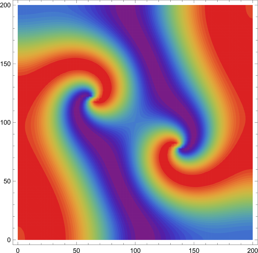
(b) $\mbox{Im}(\hat{\psi})$

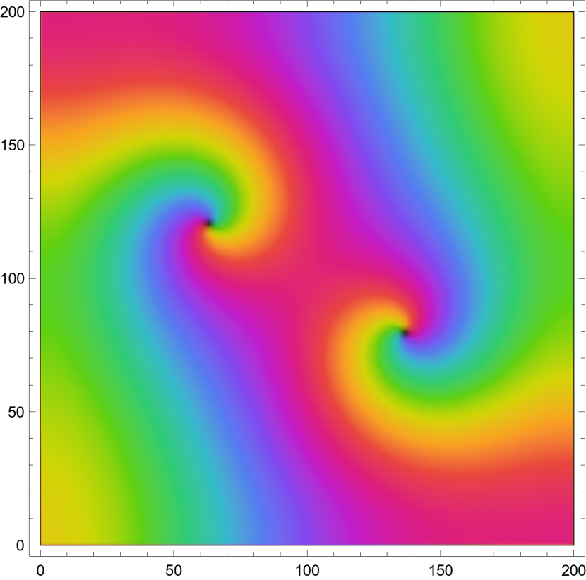
(c) $\arg(\hat{\psi})$

Figure 1: A snapshot of a simulation with two spirals for $q=0.1$.

It was observed that this choice of initial data led to brief transients after which $\hat{\psi}$ was smooth, slowly-evolving and satisfied the boundary conditions. For the most part the transients caused only relatively small changes to the starting positions ${\bf x}_{i}$ of the spirals. However, when the near-field initial condition for $\chi$ was used with too large a value of $q$ (in which $q|\log\epsilon|$ is too close to $\pi/2$) it was observed that many more zeros of $\psi$ were generated locally during the initial transient, and that these additional spirals did not always annihilate with each other. We used this behaviour to determine when to switch from the near-field initial condition to the canonical initial condition: for a single spiral we use the near-field initial condition for $q\leq 0.3$ and the canonical initial condition for $q\geq 0.35$; for two spirals we use the near-field initial condition for $q\leq 0.2$ canonical initial condition for $q\geq 0.25$. Figure 1 shows a snapshot of the real and imagainary parts and the phase of $\hat{\psi}$ for an example with two spirals.

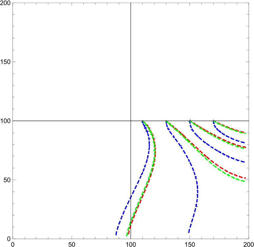
(a) $q=0.1$

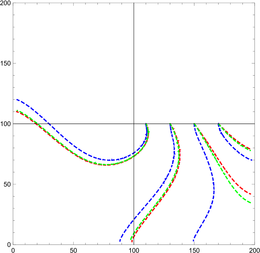
(b) $q=0.2$

Figure 2: Numerical trajectories for a single spiral starting at positions $y=100$ and $x=110$, 130, 150 and 170. The different colours correspond to different initial conditions for the phase $\chi$: blue is the canonical initial condition, red is the near-field initial condition with $\epsilon=0.01$, and green is the near-field initial condition with $\epsilon=0.005$.

In order to compare the simulations with the asymptotic predictions in Section 4.3 we need to calculate the trajectories of the spiral centres, ${\bf x}_{i}(t)$. From the simulations, at regularly spaced times, $t_{j}$, the positions of local minima of $|\psi|$ were interpolated to sub-grid resolution by fitting computed values at grid points surrounding the discrete minimum to a paraboloid. In Figure 2 we show some examples of the trajectories obtained from this procedure, for a single $+1$ spiral with various starting positions. This figure illustrates the effect that the initial condition on the phase $\chi$ can have on the trajectory of the spiral. It also illustrates a difficulty we will have when comparing our asymptotic trajectories to the numerically determined trajectories: because trajectories from nearby initial conditions are diverging, any small differences in the velocities will be compounded over time so that small errors in velocity may lead to large errors in position and quite different paths.

In Figure 3 we show a comparison between the numerically determined velocity (by finite differencing and smoothing [4] the numerically determined path in time) and the velocity predicted by the uniform asymptotic approximation described above, as a function of time along the numerically determined spiral trajectory. The numerical solutions are for a single $+1$ spiral in the square domain $0\leq x,y\leq 200$ with grid resolution $\Delta x=0.5$. For each value of $q$ the $x$ and $y$ velocities for two different trajectories (i.e. two different starting positions) are shown. The asymptotic results are shown for the two choices of $\epsilon$ described in §4.4. We see that there are still some initial transients in the velocities, but that on the whole the asymptotic approximation does quite well. The approximation gets better as $q$ increases, which seems slightly counter-intuitive since the asymptotic approximation is in the limit $q\rightarrow 0$. This can be explained by the fact that in the near-field scaling the $1/\log\epsilon$ correction terms play a more significant role than they do in the canonical scaling (in the canonical region $\epsilon$ disappears from the law of motion when written in terms of the original variables, while in the near field region it does not). From Figure 3 we also see that the green curves, corresponding to choosing $\epsilon=0.01$, fit less well at higher values of $q$, particularly near the end of the trajectory in which the spiral is approaching the boundary. On the other hand the blue curves, which take the distance to the boundary into account in $\epsilon$ through (80), fit very well.

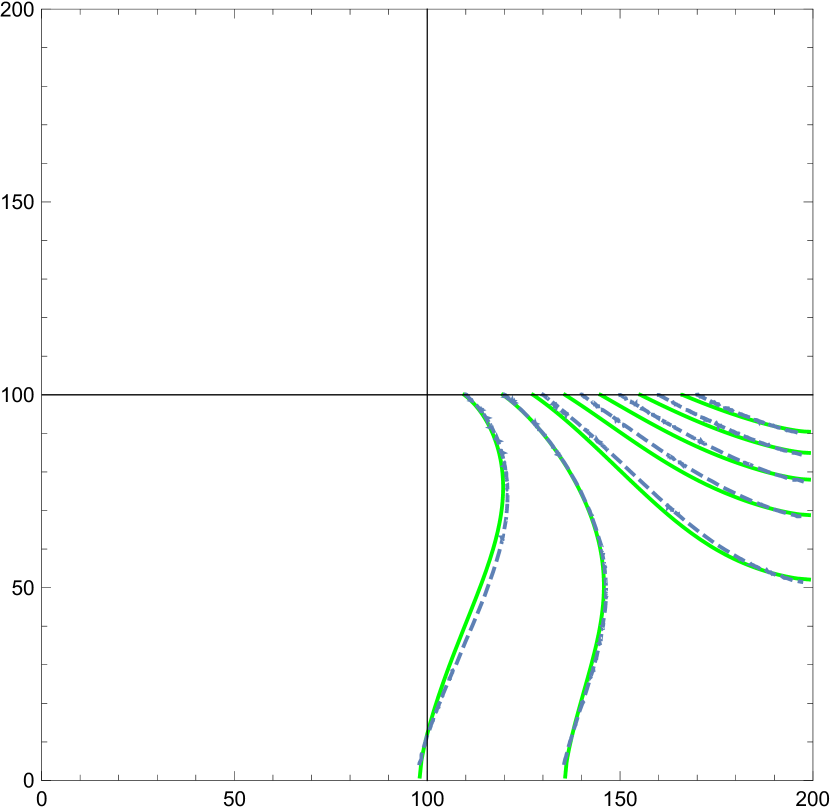
(a) $q=0.1$ Near field IC

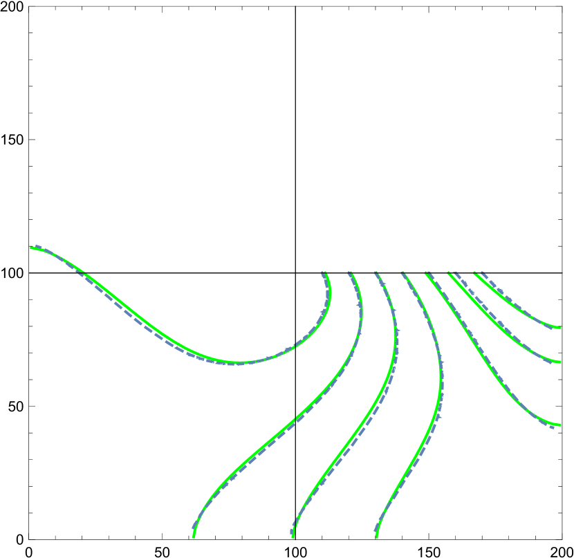
(b) $q=0.2$ Near Field IC

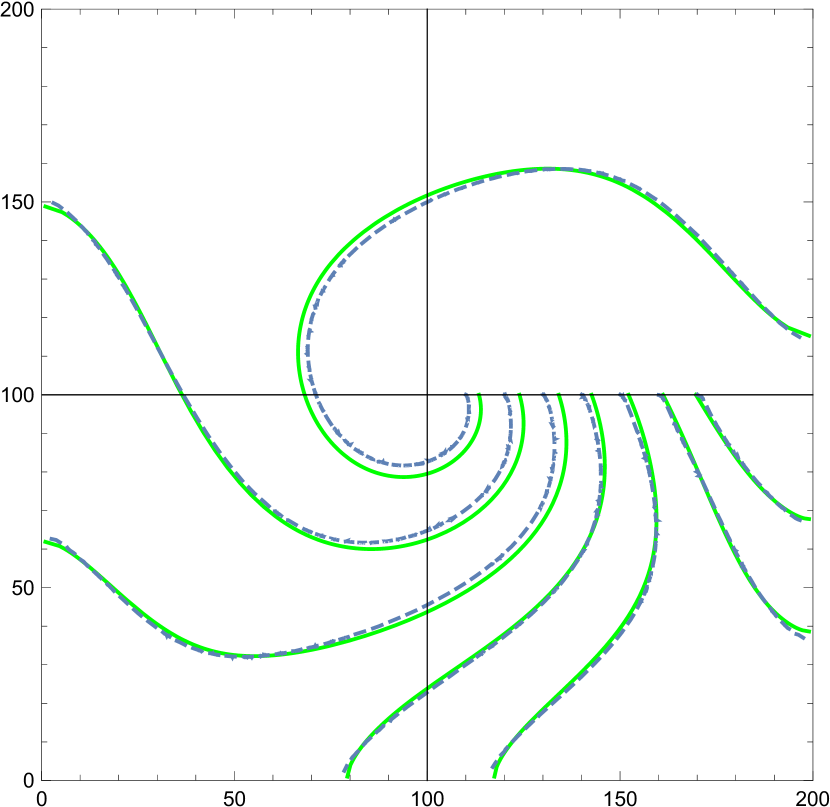
(c) $q=0.3$ Near Field IC

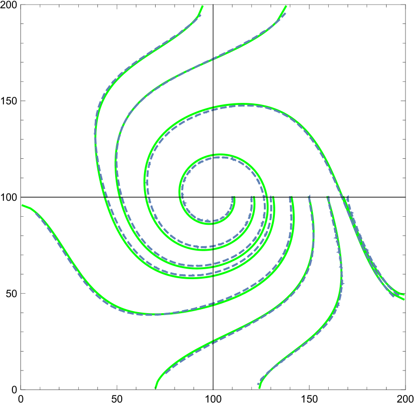
(d) $q=0.35$ Canonical IC

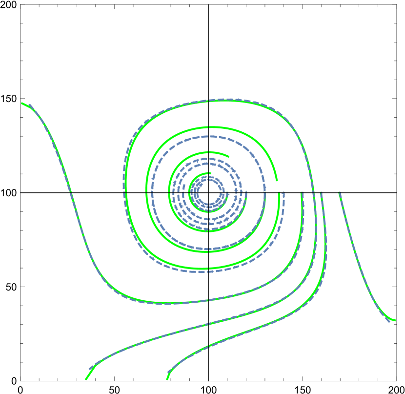
(e) $q=0.4$ Canonical IC

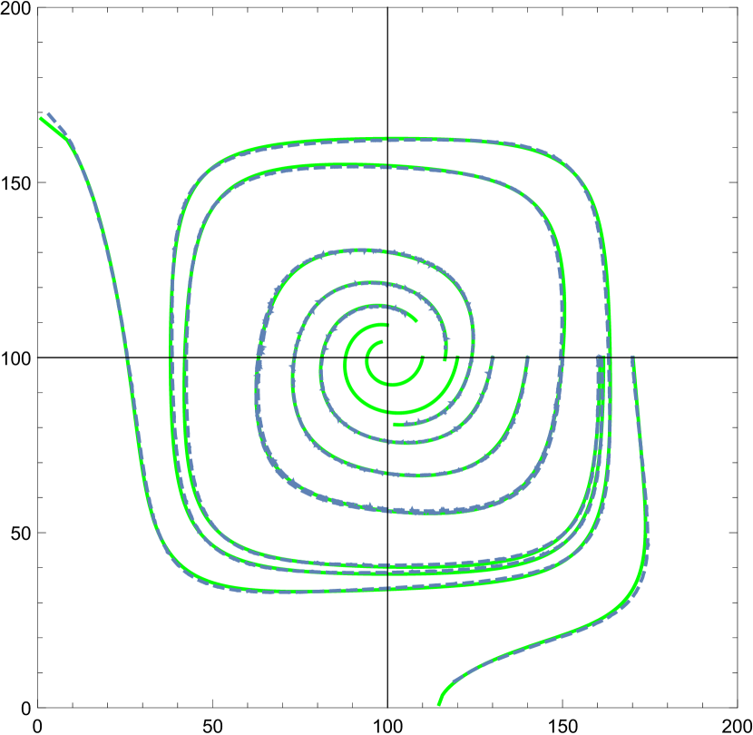
(f) $q=0.45$ Canonical IC

Figure 4: Comparison between the trajectories provided by a direct numerical simulation of (82) (dashed lines) and the uniform asymptotic approximation of §4.3 (solid lines) for a single spiral in a square domain of side 200. Numerical trajectories starting from positions $(110,100),(120,100),\ldots,(170,100)$ are shown; $\epsilon$ is given by (80). Note the appearance of an unstable periodic orbit in (4(e)) and (4(f)) which is captured by the asymptotic law of motion. An extra orbit starting from position (161,100) is shown in (f)—the periodic orbit crosses the line $x=100$ somewhere between 160 and 161.

In Figure 4 we compare directly the numerical trajectories (dashed lines) and those given by the uniform asymptotic approximation with $\epsilon$ given by (80) (solid lines), for a single $+1$ spiral in a square domain $0\leq x,y\leq 200$. Numerical trajectories are shown starting from positions $(110,100),(120,100),\ldots,(170,100)$. Because of the initial transients in the numerical results, and to mitigate the effects of diverging trajectories mentioned earlier, we solve the asymptotic trajectories backwards from a point on the numerical trajectory near the boundary of the domain. Specifically we find the asymptotic trajectory which coincides with the numerical trajectory on the smooth closed curve $(x-100)^{4}+(y-100)^{4}=90^{4}$.

For small $q$ we see that the spiral is attracted to the boundary whatever its inital position. However, as $q$ is increased there is a Hopf bifurcation with the appearance of an unstable periodic orbit. Trajectories starting outside this periodic orbit are attracted to the boundary of the domain, but those starting inside it spiral in to the origin. As $q$ is increased further the periodic orbit grows in size and develops a more squareish shape. This can be understood as the spiral interacting with its images predominantly in the near-field limit, in which the motion is perpendicular to the line of centres. With the motion dominated by the nearest image the spiral will move parallel to the nearest boundary until it nears the corner, when a second image takes over. We see that the asymptotic law of motion captures the appearance of the perioidic orbit. In Fig. 4(e) the amplitude of the asympotic periodic orbit is not quite right (it crosses the line $y=100$ close to $x=110$ rather than $x=130$), but in Fig. 4(f) the periodic orbit is captured well quantitatively as well as qualitatively.

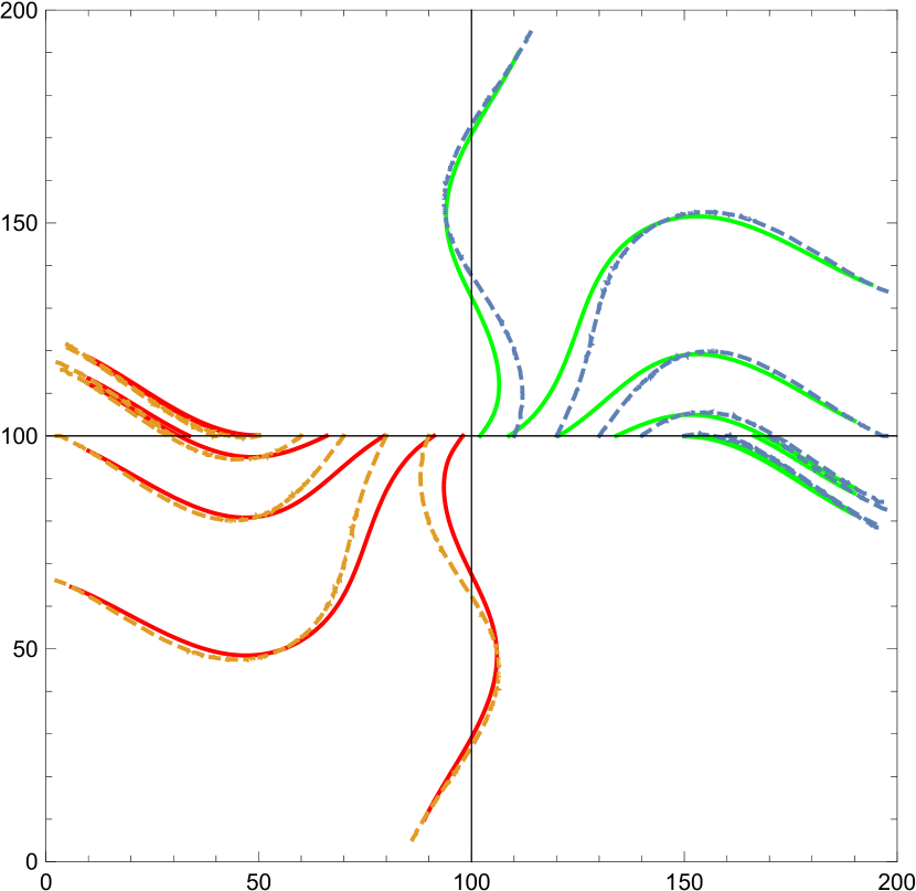
(a) $q=0.2$ near field

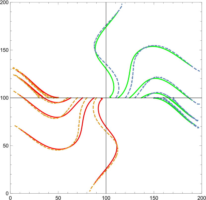
(b) $q=0.25$

(c) $q=0.3$

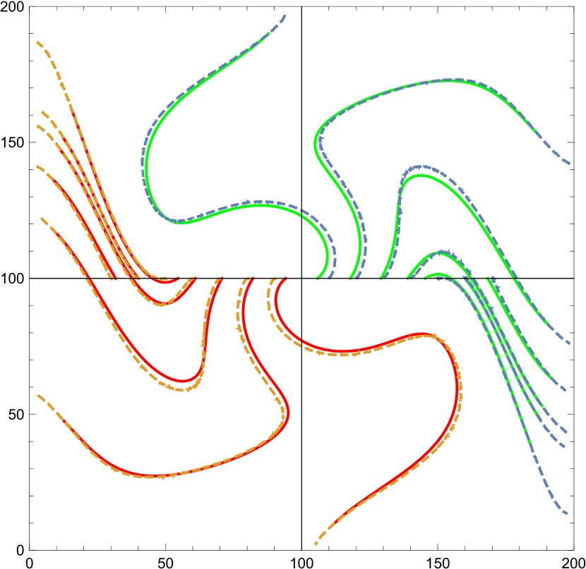
(d) $q=0.35$

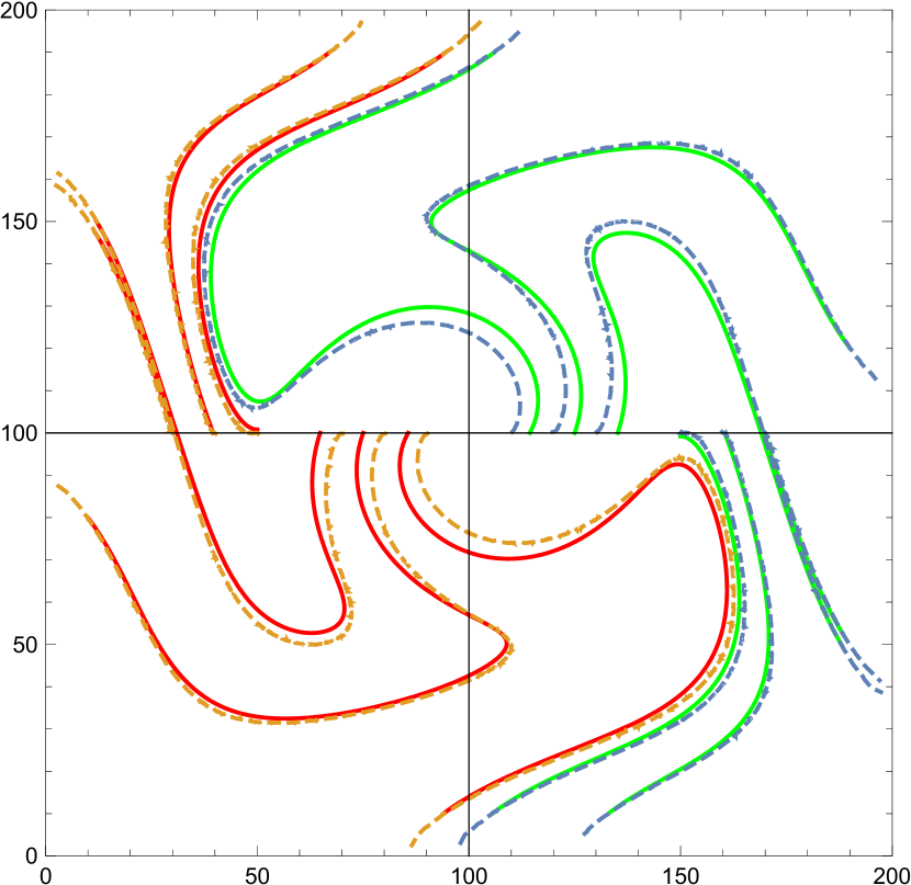
(e) $q=0.4$

Figure 5: Comparison between the trajectories provided by a direct numerical simulation of (82) (dashed lines) and the uniform asymptotic approximation of §4.3 (solid lines) for a pair of spirals in a square domain of side 200. Spirals are placed symmetrically at positions $(100-x,100)$ and $(100+x,100)$ with $x=10,20,\ldots,70$; $\epsilon$ is given by (81).

In Figure 5 we compare the trajectories provided by a direct numerical simulation of (5) (dashed lines) and those given by the uniform asymptotic approximation (solid lines) for a pair of +1 spirals in the same square domain $0\leq x,y\leq 200$. We position the spirals symmetrically at positions $(100-x,100)$ and $(100+x,100)$, where we choose $x=10,20,\ldots,70$. We see that the agreement is qualitatively very good, again improving as $q$ increases. The spirals attempt to circle around each other, as the near-field interaction would indicate, but gradually drift apart until the image spirals take over and force the pair to rotate in the opposite direction.

6 Conclusions

We have developed a law of motion for interacting spiral waves in a bounded domain in the limit that the twist parameter $q$ is small. We find that the size of the domain is crucial in determining the form of this law of motion. Our main results can be summarised as follows. For $0<q\ll 1$, given a set of $\pm 1$-armed spirals in a domain of diameter $O(1/\epsilon)$, the positions $\mathbf{x}_{\ell}$ of the spirals evolve according to the following laws of motion:

(i) For a so-called canonical domain size, which corresponds to $q|\log\epsilon|=\pi/2+q\nu$ with $\nu=O(1)$ as $q,\epsilon\rightarrow 0$,

$$\frac{\mathrm{d}\mathbf{x}_{\ell}}{\mathrm{d}t} = \frac{4\pi qn_{\ell}}{\beta_{\ell}}\sum_{j=1,j\not=\ell}^{N}\beta_{j}\nabla^{\perp}G^{\prime}_{\mathrm{n}}(\mathbf{x}_{\ell};\mathbf{x}_{j})+4\pi qn_{\ell}\nabla^{\perp}G^{\prime}_{\mathrm{n,reg}}(\mathbf{x}_{\ell};\mathbf{x}_{\ell})$$ (83)

where $\nabla^{\perp}=(-\partial_{y},\partial_{x})$ and $G^{\prime}_{\mathrm{n}}(\mathbf{x};\mathbf{y})$ is the Neumann Green’s function for the modified Helmholtz equation on $\Omega$, satisfying

$$\nabla^{2}G^{\prime}_{\mathrm{n}}-q^{2}k^{2}G^{\prime}_{\mathrm{n}}=\delta(\mathbf{x}-\mathbf{y})\quad\textrm{in}\quad\Omega,\qquad\frac{\partial G^{\prime}_{\mathrm{n}}}{\partial n}=0\quad\textrm{on}\quad\partial\Omega.$$ (84)

with

$$G^{\prime}_{\mathrm{n,reg}}(\mathbf{x};\mathbf{y})=G^{\prime}_{\mathrm{n}}(\mathbf{x};\mathbf{y})-\frac{1}{2\pi}\log|\mathbf{x}-\mathbf{y}|.$$

The coefficients $\beta_{\ell}$ are given (up to an arbitrary and irrelevant scaling factor) as solutions of the linear system of equations

$$2\pi\beta_{\ell}G^{\prime}_{\mathrm{n,reg}}(\mathbf{x}_{\ell};\mathbf{x}_{\ell})+2\pi\sum_{j=1,j\not=\ell}^{N}\beta_{j}G^{\prime}_{\mathrm{n}}(\mathbf{x}_{\ell};\mathbf{x}_{j})-\beta_{\ell}(c_{1}-\pi/2q)=0,$$ (85)

where $c_{1}\approx 0.098$, whose solvability condition (the condition for a non-zero solution) determines the eigenvalue $k$.

(ii) For a so-called near-field domain size, which corresponds to $0<q|\log\epsilon|<\pi/2$,

$$\frac{\mathrm{d}\mathbf{x}_{\ell}}{\mathrm{d}t} = 4\pi qn_{\ell}\sum_{j=1,j\not=\ell}^{N}\nabla^{\perp}\overline{G}^{\prime}_{\mathrm{n}}(\mathbf{x}_{\ell};\mathbf{x}_{j})+4\pi qn_{\ell}\nabla^{\perp}\overline{G}^{\prime}_{\mathrm{n,reg}}(\mathbf{x}_{\ell};\mathbf{x}_{\ell})$$ (86)

$$\mbox{ }-4\pi q\cot(q\log\epsilon)\nabla\overline{G}^{\prime}_{\mathrm{d,reg}}(\mathbf{x}_{\ell};\mathbf{x}_{\ell})-\frac{4\pi q\cot(q\log\epsilon)}{n_{\ell}}\sum_{j=1,j\not=\ell}^{N}n_{j}\nabla\overline{G}^{\prime}_{\mathrm{d}}(\mathbf{x}_{\ell};\mathbf{x}_{j}),\qquad$$

where $\overline{G}^{\prime}_{\mathrm{n}}(\mathbf{x};\mathbf{y})$ and $\overline{G}^{\prime}_{\mathrm{n}}(\mathbf{x};\mathbf{y})$ are the Neumann and Dirichlet Green’s functions for Laplace’s equation on $\Omega$, satisfying

$$\nabla^{2}\overline{G}^{\prime}_{\mathrm{n}} =\delta(\mathbf{x}-\mathbf{y})-\frac{1}{|\Omega|}\quad\textrm{ in }\Omega, \qquad\quad\frac{\partial\overline{G}^{\prime}_{\mathrm{n}}}{\partial{n}} =0\quad\textrm{ on }\partial\Omega,$$ (87)

$$\nabla^{2}\overline{G}^{\prime}_{\mathrm{d}} =\delta(\mathbf{x}-\mathbf{y})\quad\textrm{ in }\Omega, \qquad\quad\overline{G}^{\prime}_{\mathrm{d}} =0\quad\textrm{ on }\partial\Omega,$$ (88)

and

$$\overline{G}^{\prime}_{\mathrm{n,reg}}(\mathbf{x};\mathbf{y})=\overline{G}^{\prime}_{\mathrm{n}}(\mathbf{x};\mathbf{y})-\frac{1}{2\pi}\log|\mathbf{x}-\mathbf{y}|,\qquad\overline{G}^{\prime}_{\mathrm{d,reg}}(\mathbf{x};\mathbf{y})=\overline{G}^{\prime}_{\mathrm{d}}(\mathbf{x};\mathbf{y})-\frac{1}{2\pi}\log|\mathbf{x}-\mathbf{y}|.$$

(iii) A uniform approximation, valid in both regions, is given by

$$\frac{\mathrm{d}\mathbf{x}_{\ell}}{\mathrm{d}t} = \frac{4\pi qn_{\ell}}{\beta_{\ell}}\sum_{j=1,j\not=\ell}^{N}\beta_{j}\nabla^{\perp}G^{\prime}_{\mathrm{n}}(\mathbf{x}_{\ell};\mathbf{x}_{j})+4\pi qn_{\ell}\nabla^{\perp}G^{\prime}_{\mathrm{n,reg}}(\mathbf{x}_{\ell};\mathbf{x}_{\ell})$$ (89)

$$\mbox{ }-4\pi q\cot(q\log\epsilon)\nabla G^{\prime}_{\mathrm{d,reg}}(\mathbf{x}_{\ell};\mathbf{x}_{\ell})-\frac{4\pi q\cot(q\log\epsilon)}{n_{\ell}}\sum_{j=1,j\not=\ell}^{N}n_{j}\nabla G^{\prime}_{\mathrm{d}}(\mathbf{x}_{\ell};\mathbf{x}_{j}),\qquad$$

where $G^{\prime}_{\mathrm{d}}$ is the Dirichlet Green’s function for the modified Helmholtz equation given by

$$\nabla^{2}G^{\prime}_{\mathrm{d}}-q^{2}k^{2}G^{\prime}_{\mathrm{d}} =\delta(\mathbf{x}-\mathbf{y})\quad\textrm{in}\quad\Omega, \qquad G^{\prime}_{\mathrm{d}} =0\quad\textrm{on}\quad\partial\Omega,$$ (90)

with

$$G^{\prime}_{\mathrm{d,reg}}(\mathbf{x};\mathbf{y})=G^{\prime}_{\mathrm{d}}(\mathbf{x};\mathbf{y})-\frac{1}{2\pi}\log|\mathbf{x}-\mathbf{y}|,$$

and $\beta_{\ell}$ and $k$ given by (85).

Although we have focussed on Neumann boundary conditions for the complex Ginzburg-Landau equation (4), the extension to periodic boundary conditions is straightforward.

Acknowledgements

M. Aguareles is part of the Catalan Research group 2017 SGR 1392 and has been supported by the MINECO grant MTM2017-84214-C2-2-P (Spain). She would also like to thank the Oxford Centre for Industrial and Applied Mathematics, where part of this research was carried out.

(a) $\mbox{Re}(\hat{\psi})$

\begin{overpic}[width=212.47617pt]{q100ic20w200x-eps-converted-to.pdf} \put(0.0,21.0){{\tiny$\dot{x}_{1}$}} \put(93.0,11.0){{\tiny$t$}} \end{overpic}

\begin{overpic}[width=212.47617pt]{q100ic20w200y-eps-converted-to.pdf} \put(0.0,55.0){{\tiny$\dot{y}_{1}$}} \put(92.0,-5.0){{\tiny$t$}} \end{overpic}

(a) $q=0.1$, $x_{1}(0)=120$

\begin{overpic}[width=212.47617pt]{q200ic20w200x-eps-converted-to.pdf} \put(0.0,0.0){{\tiny$\dot{x}_{1}$}} \put(93.0,40.0){{\tiny$t$}} \end{overpic}

\begin{overpic}[width=212.47617pt]{q200ic20w200y-eps-converted-to.pdf} \put(0.0,0.0){{\tiny$\dot{y}_{1}$}} \put(92.0,-5.0){{\tiny$t$}} \end{overpic}

(b) $q=0.2$, $x_{1}(0)=120$

\begin{overpic}[width=212.47617pt]{q300ic20w300x-eps-converted-to.pdf} \put(0.0,0.0){{\tiny$\dot{x}_{1}$}} \put(93.0,41.0){{\tiny$t$}} \end{overpic}

\begin{overpic}[width=212.47617pt]{q300ic20w300y-eps-converted-to.pdf} \put(0.0,10.0){{\tiny$\dot{y}_{1}$}} \put(92.0,2.0){{\tiny$t$}} \end{overpic}

(c) $q=0.3$, $x_{1}(0)=120$

\begin{overpic}[width=212.47617pt]{q350ic20w100x-eps-converted-to.pdf} \put(0.0,4.0){{\tiny$\dot{x}_{1}$}} \put(93.0,4.0){{\tiny$t$}} \end{overpic}

\begin{overpic}[width=212.47617pt]{q350ic20w100y-eps-converted-to.pdf} \put(0.0,40.0){{\tiny$\dot{y}_{1}$}} \put(92.0,30.0){{\tiny$t$}} \end{overpic}

(d) $q=0.35$, $x_{1}(0)=120$

\begin{overpic}[width=212.47617pt]{q400ic20w400x-eps-converted-to.pdf} \put(0.0,28.0){{\tiny$\dot{x}_{1}$}} \put(95.0,20.0){{\tiny$t$}} \end{overpic}

\begin{overpic}[width=212.47617pt]{q400ic20w400y-eps-converted-to.pdf} \put(0.0,28.0){{\tiny$\dot{y}_{1}$}} \put(92.0,20.0){{\tiny$t$}} \end{overpic}

(e) $q=0.4$, $x_{1}(0)=120$

\begin{overpic}[width=212.47617pt]{q450ic61w50x-eps-converted-to.pdf} \put(0.0,40.0){{\tiny$\dot{x}_{1}$}} \put(95.0,43.0){{\tiny$t$}} \end{overpic}

\begin{overpic}[width=212.47617pt]{q450ic61w50y-eps-converted-to.pdf} \put(0.0,18.0){{\tiny$\dot{y}_{1}$}} \put(92.0,8.0){{\tiny$t$}} \end{overpic}

(f) $q=0.45$, $x_{1}(0)=161$

Figure 3: A comparison between the numerically-determined velocity (red), the predicted asymptotic velocity with $\epsilon=0.01$ (green), and the predicted asymptotic velocity with $\epsilon$ given by (80) (blue), as a function of time along the numerically-determined spiral trajectory, for a single spiral in the square domain $[0,200]\times[0,200]$. The starting $y$-value for each trajectory is $y_{1}(0)=100$. The numerical results have been locally averaged to reduce some of the noise. The trajectories themselves may be seen in Figure 4.

Appendix A Comment on [24]

As the only published work (other than our previous papers [2, 3]) to consider the motion of spirals whose separation is not large by comparison to $\mathrm{e}^{\pi/2q}$, [24] is an important reference in the field, even though their approach does not generalise easily to more than two spirals or to bounded domains. Unfortunately it seems [24] make a number of mistakes right at the beginning of their paper. Equations (8) and (9) in [24] are incorrect, and should read

$$\eta{\rho}{\mathbf{v}}\cdot\nabla{\theta} = \nabla^{2}{\rho}+\left(1-|\nabla{\theta}|^{2}-{\rho}^{2}-\frac{v^{2}\eta^{2}}{4}\right){\rho},$$

$$-\eta{\mathbf{v}}\cdot\nabla{\rho} = 2\nabla{\theta}\cdot\nabla{\rho}+{\rho}\nabla^{2}{\theta}-q\left(1-k_{0}^{2}-{\rho}^{2}\right){\rho},$$

It seems that in [24] the authors mistakenly applied the transformation $u\rightarrow u\mathrm{e}^{-\mathrm{i}\omega t+\eta\hat{\mathbf{v}}\cdot\hat{\mathbf{x}}/2}$ rather than $u\rightarrow u\mathrm{e}^{-\mathrm{i}\omega t+\mathrm{i}\eta\hat{\mathbf{v}}\cdot\hat{\mathbf{x}}/2}$ which they had intended. Equation (10) in [24] also seems incorrect, and should instead read

$$\omega=\frac{\eta-q(1-k_{0}^{2})}{1+\eta q(1-k_{0}^{2})}.$$

There are further errors in deriving (14) and (15) from (8) and (9) (two sign errors in (14) and a missing term in (15)), but since (8) and (9) are themselves incorrect that is rather academic. We do not follow through the implications of these mistakes, since the configuration of spirals they consider is a special case of the much more general setting considered here, so that their results are in any case superceded by ours.

Appendix B The law of motion when $b\neq 0$

If $b\neq 0$, equation (2) reads

$$(1-\mathrm{i}b)\frac{\partial\psi}{\partial t}=\nabla^{2}\psi+(1-|\psi|^{2})\psi+\mathrm{i}q\psi(1-k^{2}-|\psi|^{2}),$$ (91)

which after writing $\psi=fe^{\mathrm{i}\chi}$ and $\alpha=kq/\epsilon$ yields the system

$$f_{t}+bf\chi_{t} = {\nabla}^{2}f-f|{\nabla}\chi|^{2}+f(1-f^{2}),$$ (92)

$$f^{2}\chi_{t}-bff_{t} = {\nabla}\cdot(f^{2}{\nabla}\chi)+qf^{2}(1-f^{2})-\frac{\epsilon^{2}\alpha^{2}}{q}f^{2}.$$ (93)

Writing $T=\mu\epsilon^{2}t$ and $\mathbf{X}=\epsilon\mathbf{x}$ the outer equations (7)-(8) now read

$$\mu\epsilon^{2}(f_{T}+bf\chi_{T}) = \epsilon^{2}{\nabla}^{2}f-\epsilon^{2}f|{\nabla}\chi|^{2}+f(1-f^{2}),$$ (94)

$$\mu\epsilon^{2}(f^{2}\chi_{T}-bff_{T}) = \epsilon^{2}{\nabla}\cdot(f^{2}{\nabla}\chi)+qf^{2}(1-f^{2})-\frac{\epsilon^{2}\alpha^{2}}{q}f^{2},$$ (95)

which, expanding in asymptotic power series in $\epsilon$ as $f\sim f_{0}+\epsilon^{2}f_{1}+\cdots$ and $\chi\sim\chi_{0}+\epsilon^{2}\chi_{1}+\cdots$, gives, in place of (9),

$$f_{0}=1,\quad f_{1}=-\frac{1}{2}\left(\mu b\chi_{0T}+|\nabla\chi_{0}|^{2}\right),$$

so that equation (10) for the leading-order (in $\epsilon$) phase becomes

$$\mu\chi_{0T}(1-qb)={\nabla}^{2}\chi_{0}+q|\nabla\chi_{0}|^{2}-\alpha^{2}/q.$$

We see that the correction due to nonzero $b$ is of $O(\mu qb)$, so that the equations for $\chi_{00}$ and $\chi_{01}$ in both the canonical scaling and the near field scaling are unchanged if $b=O(1)$.

In the inner region, if $b\not=0$, equation (16) becomes

$$\epsilon\mu(1-\mathrm{i}b)\left(\epsilon\psi_{T}-\frac{\mathrm{d}\mathbf{X}_{\ell}}{\mathrm{d}T}\cdot\nabla\psi\right)=\nabla^{2}\psi+(1+\mathrm{i}q)(1-|\psi|^{2})\psi-\mathrm{i}\frac{\epsilon^{2}\alpha^{2}}{q}\psi.$$

The leading order equation (17) is unchanged, while the first order equation (20) becomes

$$-\mu(1-\mathrm{i}b)\frac{\mathrm{d}\mathbf{X}_{\ell}}{\mathrm{d}T}\cdot\nabla\psi_{0}=\nabla^{2}\psi_{1}+(1+\mathrm{i}q)(\psi_{1}(1-2|\psi_{0}|^{2})-\psi_{0}^{2}\psi_{1}^{*}).$$

or equivalently, in terms of $f_{1}$ and $\chi_{1}$,

$$-\mu\frac{\mathrm{d}\mathbf{X}_{\ell}}{\mathrm{d}T}\cdot\left(\nabla f_{0}+bf_{0}\nabla\chi_{0}\right) = \nabla^{2}f_{1}-f_{1}|\nabla\chi_{0}|^{2}-2f_{0}\nabla\chi_{0}\cdot\nabla\chi_{1}+f_{1}-3f_{0}^{2}f_{1},$$

$$-\mu f_{0}\frac{\mathrm{d}\mathbf{X}_{\ell}}{\mathrm{d}T}\cdot\left(f_{0}\nabla\chi_{0}-b\nabla f_{0}\right) = \nabla\cdot(f_{0}^{2}\nabla\chi_{1})+\nabla\cdot(2f_{0}f_{1}\nabla\chi_{0})+2qf_{0}f_{1}-4qf_{0}^{3}f_{1}.$$

When calculating the outer limit of the first order inner equation (33) is now modified to

$$-\mu(1-qb)\frac{\mathrm{d}\mathbf{X}_{\ell}}{\mathrm{d}T}\cdot\nabla\widehat{\chi}_{00}={\nabla}^{2}\widehat{\chi}_{01}+2q\nabla\widehat{\chi}_{00}\cdot\nabla\widehat{\chi}_{10}.$$

It is now clear that when $b$ is $O(1)$ as $q\rightarrow 0$, a non-zero $b$ modifies the law of motion only at $O(q)$, not at leading order. To have an effect on the leading-order law of motion $b$ needs to be $O(1/q)$. We outline here the modification to our calculations in this latter case, and the resulting modified law of motion.

Writing $b=\tilde{b}/q$, $\mu=\tilde{\mu}q$, the outer equation (6) reads

$$\epsilon^{2}\tilde{\mu}\left(q-\mathrm{i}\tilde{b}\right)\psi_{T}=\epsilon^{2}\nabla^{2}\psi+(1+\mathrm{i}q)(1-|\psi|^{2})\psi-\frac{\mathrm{i}\epsilon^{2}\alpha^{2}}{q}\psi,$$ (96)

and (7)-(8) in terms of the modulus $f$ and phase $\chi$ become

$$\tilde{\mu}\epsilon^{2}(qf_{T}+\tilde{b}f\chi_{T}) =\epsilon^{2}\nabla^{2}f-\epsilon^{2}f|\nabla\chi|^{2}+(1-f^{2})f,$$ (97)

$$\tilde{\mu}\epsilon^{2}(qf^{2}\chi_{T}-\tilde{b}ff_{T}) =\epsilon^{2}\nabla\cdot(f^{2}\nabla\chi)+qf^{2}(1-f^{2})-\epsilon^{2}\frac{\alpha^{2}}{q}f^{2}.$$ (98)

Expanding $\chi$ and $f$ in powers of $\epsilon$ we find that equation (10) for leading-order phase becomes

$$q\tilde{\mu}\chi_{0T}(1-\tilde{b})=\nabla^{2}\chi_{0}+q|\nabla\chi_{0}|^{2}-\alpha^{2}/q.$$

Expanding in powers of $q$ as usual we find that the terms involving $\tilde{b}$ still do not contribute at the relevant order in either the near-field or canonical separation.

In the inner region the leading-order equation (17) is unchanged, while the first-order equation (20) becomes

$$-\tilde{\mu}(q-\mathrm{i}\tilde{b})\frac{\mathrm{d}\mathbf{X}_{\ell}}{\mathrm{d}T}\cdot\nabla\psi_{0}=\nabla^{2}\psi_{1}+(1+\mathrm{i}q)(\psi_{1}(1-2|\psi_{0}|^{2})-\psi_{0}^{2}\psi_{1}^{*}).$$

or equivalently, in terms of $f_{1}$ and $\chi_{1}$,

$$-\tilde{\mu}\frac{\mathrm{d}\mathbf{X}_{\ell}}{\mathrm{d}T}\cdot\left(q\nabla f_{0}+\tilde{b}f_{0}\nabla\chi_{0}\right) = \nabla^{2}f_{1}-f_{1}|\nabla\chi_{0}|^{2}-2f_{0}\nabla\chi_{0}\cdot\nabla\chi_{1}+f_{1}-3f_{0}^{2}f_{1},$$

$$-\tilde{\mu}f_{0}\frac{\mathrm{d}\mathbf{X}_{\ell}}{\mathrm{d}T}\cdot\left(qf_{0}\nabla\chi_{0}-\tilde{b}\nabla f_{0}\right) = \nabla\cdot(f_{0}^{2}\nabla\chi_{1})+\nabla\cdot(2f_{0}f_{1}\nabla\chi_{0})+2qf_{0}f_{1}-4qf_{0}^{3}f_{1}.$$

When calculating the outer limit of the first-order inner equation (33) is now modified to

$$-q\tilde{\mu}(1-\tilde{b})\frac{\mathrm{d}\mathbf{X}_{\ell}}{\mathrm{d}T}\cdot\nabla\widehat{\chi}_{00}={\nabla}^{2}\widehat{\chi}_{01}+2q\nabla\widehat{\chi}_{00}\cdot\nabla\widehat{\chi}_{10}.$$

so that the solution (35) is modified to

$$\widehat{h}_{1} = -\frac{q\tilde{\mu}(1-\tilde{b})A_{\ell}\epsilon^{-\mathrm{i}qn_{\ell}}(V_{1}-\mathrm{i}V_{2})}{4}(R^{\mathrm{i}qn_{\ell}+1}+\gamma_{1}R^{1-\mathrm{i}qn_{\ell}})\,\mathrm{e}^{(qn_{\ell}+\mathrm{i})\phi}$$ (99)

$$\mbox{ }-\frac{q\tilde{\mu}(1-\tilde{b})B_{\ell}\epsilon^{\mathrm{i}qn_{\ell}}(V_{1}+\mathrm{i}V_{2})}{4}(R^{-\mathrm{i}qn_{\ell}+1}+\gamma_{2}R^{1+\mathrm{i}qn_{\ell}})\,\mathrm{e}^{(qn_{\ell}-\mathrm{i})\phi}.$$

where

$$\widehat{\chi}_{10}=\frac{\widehat{h}_{1}e^{-q\widehat{\chi}_{00}}}{q}.$$

At this point the analysis for spirals at canonical separation and those at near field separation differs, and we treat the two cases separately.

Canonical separation

Since the leading-order inner equation is independent of $\tilde{b}$, the leading-order matching is the same, giving $q\log(1/\epsilon)=\pi/2+\nu q$ as before. Matching the new solution (99) to the inner limit of the outer as in §2.6 we find that (41) becomes

$$\chi_{10}\sim-\frac{\tilde{\mu}(1-\tilde{b})r}{2}(V_{1}\cos\phi+V_{2}\sin\phi)+\frac{n_{\ell}r}{\beta_{\ell}}\nabla{\cal G}^{\ell}_{\mathrm{reg}}(\mathbf{X}_{\ell})\cdot{\bf e}_{\phi}\qquad\mbox{ as }r\rightarrow\infty.$$

The solvability condition (43) is modified to

$$-\tilde{\mu}\tilde{b}\pi\frac{\mathrm{d}{\bf X}_{\ell}}{\mathrm{d}T}\cdot{\bf d^{\perp}}=\lim_{r\rightarrow\infty}\int_{0}^{2\pi}({\bf e}_{\phi}\cdot{\bf d})\left(\frac{\partial\chi_{10}}{\partial r}+\frac{\chi_{10}}{r}\right)\,\mathrm{d}\phi,$$ (100)

where ${\bf d}^{\perp}=(-d_{2},d_{1})$. The terms in $\tilde{b}$ cancel, leaving the law of motion unchanged as

$$\frac{\mathrm{d}{\bf X}_{\ell}}{\mathrm{d}T}=-\frac{2n_{\ell}}{\tilde{\mu}\beta_{\ell}}\,\nabla^{\perp}{\cal G}^{\ell}_{\mathrm{reg}}(\mathbf{X}_{\ell}).$$

We note that in [3] there is a sign error which resulted in the terms involving $\tilde{b}$ adding up rather than cancelling, leading to an incorrect factor $1-2\tilde{b}$ in the law of motion.

Near field separation

In this case the computations follow similarly to the ones shown for the canonical separation. In particular, with $\tilde{b}$ non-zero the first order matching between the inner limit of the outer and outer limit of the inner (69) becomes

$$\bar{\mathbf{x}}\cdot\nabla\overline{\cal G}^{\ell}_{\mathrm{reg}}(\mathbf{X}_{\ell}) \sim -\frac{\tilde{\mu}(1-\tilde{b})}{4}\left(\frac{\mathrm{e}^{-\mathrm{i}qn_{\ell}\log\epsilon}(V_{1}-\mathrm{i}V_{2})(1+\gamma_{1})r\mathrm{e}^{\mathrm{i}\phi}}{\mathrm{e}^{-\mathrm{i}qn_{\ell}\log\epsilon}+\mathrm{e}^{\mathrm{i}qn_{\ell}\log\epsilon}}+\frac{\mathrm{e}^{\mathrm{i}qn_{\ell}\log\epsilon}(V_{1}+\mathrm{i}V_{2})(1+\gamma_{2})r\mathrm{e}^{-\mathrm{i}\phi}}{\mathrm{e}^{-\mathrm{i}qn_{\ell}\log\epsilon}+\mathrm{e}^{\mathrm{i}qn_{\ell}\log\epsilon}}\right).$$

Solving for $\gamma_{1}$ and $\gamma_{2}$ and matching in the same way as done in §3.6 now gives

$$\chi_{10} \sim -\frac{\tilde{\mu}(1-\tilde{b})r}{4}\left(V_{1}\cos\phi+V_{2}\sin\phi\right)$$

$$+\frac{\tilde{\mu}(1-\tilde{b})r}{4}\left(V_{1}\cos(\phi-2qn_{\ell}\log\epsilon)+V_{2}\sin(\phi-2qn_{\ell}\log\epsilon)\right)$$

$$+r\cos(qn_{\ell}\log\epsilon)\left(\frac{\partial\overline{\cal G}^{\ell}_{\mathrm{reg}}}{\partial X}({\bf X}_{\ell})\cos(\phi-qn_{\ell}\log\epsilon)+\frac{\partial\overline{\cal G}^{\ell}_{\mathrm{reg}}}{\partial Y}({\bf X}_{\ell})\sin(\phi-qn_{\ell}\log\epsilon)\right).$$

Then, using the solvability condition (100), the law of motion reads

$$\frac{\mathrm{d}{\bf X}_{\ell}}{\mathrm{d}T} = \frac{2\cos(qn_{\ell}\log\epsilon)}{\tilde{\mu}(\tilde{b}^{2}\cos^{2}(qn_{\ell}\log\epsilon)+\sin^{2}(qn_{\ell}\log\epsilon))}\left(\tilde{b}\cos(qn_{\ell}\log\epsilon)\nabla{\cal G}^{\ell}_{\mathrm{reg}}(\mathbf{X}_{\ell})\right.$$

$$\left.\hskip 199.16928pt+\sin(qn_{\ell}\log\epsilon)\nabla^{\perp}{\cal G}^{\ell}_{\mathrm{reg}}(\mathbf{X}_{\ell})\right).$$

Again we note that the corresponding expression for an infinite domain in [3] is incorrect because of the aforementioned sign error.

References

- [1] M. Aguareles. The effect of boundaries on the asymptotic wavenumber of spiral wave solutions of the complex Ginzburg–Landau equation. Phys. D, 278(1):1–12, 2014.
- [2] M. Aguareles, S. J. Chapman, and T. Witelski. Interaction of spiral waves in the complex ginzburg-landau equation. Phys. Rev. Lett., 101:art. no. 224101, 2008.
- [3] M. Aguareles, S. J. Chapman, and T. Witelski. Motion of spiral waves in the complex Ginzburg-Landau equation. Phys. D, 239(7):348–365, 2010.
- [4] R. S. Anderssen and F. R. D. Hoog. Finite difference methods for the numerical differentiation of non-exact data. Computing, 33(3-4):256–267, 1984.
- [5] I. Aranson, L. Kramer, and A. Weber. On the interaction of spiral waves in non-equilibrium media. Phys. D, 53(3):376–394, 1991.
- [6] I. Aranson, L. Kramer, and A. Weber. Theory of interaction and bound states of spiral waves in oscillatory media. Phys. Rev. E, 47(4):3231–3241, 1993.
- [7] I. S. Aranson and L. Kramer. The world of the complex Ginzburg-Landau equation. Rev. Modern Phys., 74(1):99–143, 2002.
- [8] M. Barkley, M. Kness, and L. S. Tuckerman. Spiral-wave dynamics in a simple model of excitable media: the transition from simple to compound rotation. Phys. Rev. A, 42(4):2489–2492, 1990.
- [9] V. N. Biktashev. Drift of a reverberator in an active medium due to the interaction with boundaries. In A. V. Gaponov-Grekhov, M. I. Rabinovich, and J. Engelbrecht, editors, Nonlinear Waves. Dynamics and Evolution, pages 87–96. Springer, Berlin, 1989.
- [10] T. Bohr, G. Huber, and E. Ott. The structure of spiral-domain patterns and shocks in the D complex Ginzburg-Landau equation. Phys. D, 106(1-2):95–112, 1997.
- [11] C. Brito, I. S. Aranson, and H. Chaté. Vortex glass and vortex liquid in oscillatory mdeia. Phys. Rev. Lett., 90(6), 2003.
- [12] S. K. Das. Unlocking of frozen dynamics in the complex Ginzburg-Landau equation. Phys. Rev. E, 87(1):012135, 2013.
- [13] M. Dowle, R. M. Mantel, and D. Barkley. Fast simulations of waves in three-dimensional excitable media. Int. J. of Bif. and Chaos, 7(11):2529–2545, 1997.
- [14] J. M. Greenberg. Spiral waves for systems. SIAM J. Appl. Math., 39(2):536–547, 1980.
- [15] P. S. Hagan. Spiral waves in reaction-diffusion equations. SIAM J. Appl. Math., 42(4):762–786, 1982.
- [16] P. C. Hohenberg and A. P. Krekhov. An introduction to the Ginzburg–Landau theory of phase transitions and nonequilibrium patterns. Physics Reports, 572:1–42, 2015.
- [17] N. Kopell and L. N. Howard. Target pattern and spiral solutions to reaction-diffusion equations with more than one space dimension. Adv. Appl. Math., 2:417–449, 1981.
- [18] Y. Kuramoto. Chemical oscillations, waves, and turbulence, volume 19 of Springer Series in Synergetics. Springer-Verlag, Berlin, 1984.
- [19] J. V. Moloney and A. C. Newell. Nonlinear optics. Phys. D, 44(1-2):1–37, 1990.
- [20] S. Mowlaei, A. Roman, and M. Pleimling. Spirals and coarsening patterns in the competition of many species: a complex Ginzburg–Landau approach. J. Phys. A, 47(16):165001, 2014.
- [21] J. C. Neu. Vortices in complex scalar fields. Phys. D, 43(2-3):385–406, 1990.
- [22] J. Paullet, B. Ermentrout, and W. Troy. The existence of spiral waves in an oscillatory reaction-diffusion system. SIAM J. Appl. Math., 54(5):1386–1401, 1994.
- [23] L. M. Pismen. Weakly radiative spiral waves. Phys. D, 184(1-4):141–152, 2003. Complexity and nonlinearity in physical systems (Tucson, AZ, 2001).
- [24] L. M. Pismen and A. A. Nepomnyashchy. On interaction of spiral waves. Phys. D, 54(3):183–193, 1992.
- [25] M. Van Dyke. Perturbation Methods in Fluid Mechanics. Parabolic Press, Stanford, CA, 1975.
- [26] R. W. Walden, P. Kolodner, A. Passner, and C. M. Surko. Traveling waves and chaos in convection in binary fluid mixtures. Phys. Rev. Lett., 55(5):496–499, Jul 1985.
- [27] A. N. Zaikin and A. M. Zhabotinsky. Concentration wave propagation in two-dimensional liquid-phase. self-oscillating system. Nature, 225:535–537, 1970.