Dispertio: Optimal Sampling for Safe
Deterministic Sampling-Based Motion Planning

Abstract

A key challenge in robotics is the efficient generation of optimal robot motion with safety guarantees in cluttered environments. Recently, deterministic optimal sampling-based motion planners have been shown to achieve good performance towards this end, in particular in terms of planning efficiency, final solution cost, quality guarantees as well as non-probabilistic completeness. Yet their application is still limited to relatively simple systems (i.e., linear, holonomic, Euclidean state spaces). In this work, we extend this technique to the class of symmetric and optimal driftless systems by presenting Dispertio, an offline dispersion optimization technique for computing sampling sets, aware of differential constraints, for sampling-based robot motion planning. We prove that the approach, when combined with PRM*, is deterministically complete and retains asymptotic optimality. Furthermore, in our experiments we show that the proposed deterministic sampling technique outperforms several baselines and alternative methods in terms of planning efficiency and solution cost.

I Introduction

Motion planning is key to intelligent robot behavior. For motion planning in safety-critical applications, where self-driving cars, social or collaborative robots operate amidst and work with humans, safety guarantees, explainability and deterministic performance bounds are of particular interest. In the past, many motion planning approaches have been introduced to improve planning efficiency, path quality and applicability across classes of robotic systems. Probabilistic sampling-based motion planners [7, 9, 6] and their optimal variants [5, 4] have shown to outperform combinatorial approaches [11], especially for high-dimensional systems with complex environments and differential constraints. Sampling-based planners explore the configuration space by sampling states and connecting them to the roadmap, or tree, which represents and keeps track of the spatial connectivity. Typically samples are drawn from a uniform distribution over the state space by an independent and identically distributed (i.i.d.) random variable. Biasing techniques towards the goal region or promising areas of the configuration space may be used if available [16, 17]. The randomness of the samples set ensures good exploration of the configuration space, but comes at the expense of stochastic results which may strongly vary for each planning query in terms of planning efficiency and path quality. This stochasticity makes the formal verification and validation of such algorithms, needed for safety-critical applications, difficult to obtain.

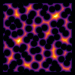
(a) Halton

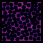
(b) Dispertio

Figure 1: Comparison of the coverage between $l_{2}$ low dispersion Halton samples and our optimized samples for a 2D Euclidean case. Bright color highlights uncovered areas. Our approach achieves better coverage than the baseline.

To address this issue, several authors [8, 3] proposed to use deterministic sets (or sequences). Contrarily to using i.i.d. random variables, this technique allows to achieve deterministic planning behaviors while still getting on par or even better performance. Moreover, as described also in [8, 3], deterministic sampling allows an easier certification process for the planners (e.g., in terms of final cost, clearance from the obstacles). Particularly, as we will see also in our case, those approaches have been shown to be complete (i.e., to find a solution) for planning queries for which a solution with certain clearance exists. However, current approaches limit their applicability to Euclidean spaces [8], systems with linear affine dynamics [3] and specific driftless ones [19].

With the goal to further enhance the usage of deterministic sampling to symmetric and optimal driftless systems, in this work we present Dispertio, an optimization-based approach to deterministic sampling. The approach computes a sampling set which minimizes the actual dispersion of the samples. To compute the dispersion metric, we need access to a steer function [15, 20] that can compute an optimal path connecting two states. We focus our attention on uninformed batch-based algorithms (e.g., PRM* [5]) where the set of samples can be precomputed offline. We prove that the approach, when combined with PRM*, is deterministically complete and retains asymptotic optimality. Furthermore, we systematically compare our approach to the existing baselines [3, 19]. The experiments demonstrate that our approach outperforms the baselines in terms of planning efficiency and overall final path quality.

Classical
grid-search

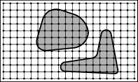
Subsampled
grid-search

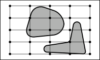
Lattice-based
grid-search

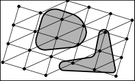
Quasi-random
roadmap

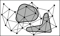
Probabilistic
roadmap

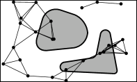
Figure 2: Range of possible sampling and roadmap types as introduced by LaValle [8]. The highlighted ones are deterministic.

II Related Work

LaValle et al. [8] highlight the relationship between grid-based and probabilistic planning, see Fig. 2. The authors advocate that grid-based planners and probabilistic sampling-based planners all belong to the same class of sampling-based algorithms and are extremes of a broad spectrum of sampling strategies, ranging from deterministic to highly stochastic techniques. They highlight the benefits of deterministic sampling sets (or sequences) such as grids [10, 13], lattices [18], or Halton and Sukharev sequences [25, 24]. In particular, LaValle et al. [1, 8] show that dispersion (see Sec. III for the definition) is the deciding metric when it comes to resolution complete path planning. The reason is that dispersion provides lower bounds on the coverage of the space. The authors prove that low dispersion sampling, using for example Halton and Sukharev sequences [25, 24], provides deterministic completeness guarantees on finding feasible paths, which i.i.d. sampling can only probabilistically provide, i.e., the planner will find a solution with a probability of 1 as the number of samples goes to infinity. Our approach follows the ideas presented by [8] and extends their results to motion planning with differential constraints.

While the authors in [8] focus on feasibility in deterministic sampling-based motion planning, Janson et al. [3] extend the approach to address optimality. The authors show that with a particular choice of low dispersion sampling ($l_{2}$ dispersion of order $O(n^{-1/D})$, e.g., Halton sequence, with $D$ being the state space dimension of the considered system), optimal sampling-based planners (i.e., PRM* [5, 21]) can use a lower connection radius compared to i.i.d. sampling thus requiring a lower computational complexity, i.e., $r_{n}\in\omega(n^{-1/D})$. Moreover, they show that the cost or suboptimality of the returned solution can be bounded, based on the dispersion. The latter work limits its applicability to Euclidean spaces and to systems having linear affine dynamics. In comparison our method can be applied also to symmetric and optimal driftless systems with differential constraints.

Poccia [19] proposes an approach for generating a set of deterministic samples for nonholonomic systems. The approach needs an explicit and careful analysis of the system equations to come up with a sampling scheme. Differently, our approach provides an algorithm that only needs the availability of an optimal steer function, a common assumption for optimal sampling-based planning [5, 21].

Unlike state-lattice approaches [18], which can be seen as part of the class of deterministic sampling-based planners, our approach does not rely on a regular grid or a set of pre-defined motion primitives. Instead, it optimizes the position of the samples based on the dispersion metric that accounts for the differential constraints of the system.

III Our Approach

In this section, we formalize the problem that we aim to solve and the novel dispersion definition. We will then describe our algorithm and analyze its properties.

III-A Problem Definition

Let $\mathcal{X}\subset\mathbb{R}^{D}$ be a manifold defining a configuration space, $\mathcal{U}\subset\mathbb{R}^{M}$ the symmetric control space, $\mathcal{X}_{\mathrm{obs}}\subset\mathcal{X}$ the obstacle space and $\mathcal{X}_{\mathrm{free}}=\mathcal{X}\setminus\mathcal{X}_{\mathrm{obs}}$ the free space. A driftless control-affine system can be described by a differential equation as

$$\dot{\boldsymbol{x}}(t)=\sum_{j=1}^{M}g_{j}(\boldsymbol{x}(t))\mathbf{u}(t)$$ (1)

where $\boldsymbol{x}(t)\in\mathcal{X}$, $\mathbf{u}(t)\in\mathcal{U}$, for all $t$, and $g_{1},\ldots,g_{M}$ being the system vector fields on $\mathcal{X}$. For the remainder of the paper we will focus on symmetric systems for which an optimal steer function exists.

Let $\gamma$ denote a planning query, defined by its initial state $\boldsymbol{x}_{\mathrm{start}}\in\mathcal{X}$ and goal state $\boldsymbol{x}_{\mathrm{goal}}\in\mathcal{X}$. We define the set of all possible solution paths for a given query $\gamma$ as $\Sigma_{\gamma}$, with $\sigma\in\Sigma_{\gamma}:[0,1]\to\mathcal{X}_{\mathrm{free}}$ being one of the possible solution paths such that $\sigma(0)=\boldsymbol{x}_{\mathrm{start}}$ and $\sigma(1)=\boldsymbol{x}_{\mathrm{goal}}$. The arc-length of a path $\sigma$ is defined by $l(\sigma)=\int_{0}^{1}||\dot{\sigma}(t)||_{2}~{}dt$. The arc-length induces a sub-Riemannian distance $\mathrm{dist}$ on $\mathcal{X}$: $\mathrm{dist}(\boldsymbol{x},\boldsymbol{z})=\inf_{\sigma}l(\sigma)$, i.e., the length of the optimal path connecting $\boldsymbol{x}$ to $\boldsymbol{z}$, which due to our assumptions is also symmetric. Let $\sigma^{*}$ denote the set of all points along a path $\sigma$. The $\mathrm{dist}$-clearance of a path $\sigma$ is defined as

$$\delta_{\mathrm{dist}}(\sigma)=\sup\big{\{}r\in\mathbb{R}~{}|~{}\mathcal{R}_{\mathrm{dist}}({\boldsymbol{x}},r)\subseteq\mathcal{X}_{\mathrm{free}}~{}\forall{\boldsymbol{x}}\in\sigma^{*}\big{\}}$$ (2)

where $\mathcal{R}_{\mathrm{dist}}({\boldsymbol{x}},r)$ is the cost-limited reachable set (closed if not otherwise stated) for the system in Eq. 1 centered at ${\boldsymbol{x}}$ within a path length of $r$ (e.g., a sphere for Euclidean systems):

$$\mathcal{R}_{\mathrm{dist}}(\boldsymbol{x},r)=\big{\{}\boldsymbol{z}\in\mathcal{X}~{}|~{}\mathrm{dist}(\boldsymbol{x},\boldsymbol{z})\leq r\big{\}}.$$ (3)

The $\mathrm{dist}$-clearance of a query $\gamma$ is defined as

$$\delta_{\mathrm{dist}}(\gamma)=\sup\big{\{}\delta_{\mathrm{dist}}(\sigma)~{}|~{}\sigma\in\Sigma_{\gamma}\big{\}}$$ (4)

and denotes the maximum clearance that a solution path to a query can have. An optimal sampling-based algorithm solves the following $\hat{\delta}_{\mathrm{dist}}$-robustly feasible motion planning problem $\mathcal{P}$: given a query $\hat{\gamma}$ with a $\mathrm{dist}$-clearance of $\delta_{\mathrm{dist}}(\hat{\gamma})>\hat{\delta}_{\mathrm{dist}}$, find a control $\mathbf{u}(t)\in\mathcal{U}$ with domain $[0,1]$ such that the unique trajectory $\sigma$ satisfies Eq. 1, is fully contained in the free space $\mathcal{X}_{\mathrm{free}}\subseteq\mathcal{X}$ and goes from $\boldsymbol{x}_{\mathrm{start}}$ to $\boldsymbol{x}_{\mathrm{goal}}$. Moreover it minimizes, asymptotically, a defined cost function $c:\Sigma_{\gamma}\rightarrow\mathbb{R}_{\geq 0}$. Hereinafter, we will use the term steer function to indicate a function that generates a path in $\mathcal{X}$ connecting two specified states. In particular we will use steer functions that solve an optimal control problem, i.e., minimizing the cost $c$.

In the following sections, we describe the approach to solve $\mathcal{P}$ by using an optimization-based sampling technique that minimizes the actual dispersion of the sampling set used by batch-processing algorithms (e.g., PRM*, see Alg. 1).

III-B Dispersion for Differentially Constrained Systems

We use and modify the dispersion definition for a sampling set $\mathcal{S}=\left\{\boldsymbol{x}_{0},\boldsymbol{x}_{1},\dots,\boldsymbol{x}_{n}\right\}\subset\mathcal{X}$, introduced by Niederreiter [14] and also adopted by [8, 3]:

$$d_{\mathrm{dist}}=\sup\{r>0~{}|~{}\exists\boldsymbol{x}\in\mathcal{X}\text{ with }\mathcal{R}_{\mathrm{dist}}(\boldsymbol{x},r)\cap\mathcal{S}=\emptyset\}.$$ (5)

Intuitively the dispersion can be considered as the radius of the largest (open) ball (i.e., size of the reachable set) that does not contain an element of $S$. In the context of differentially constrained motion planning, we propose to adjust the dispersion metric to explicitly require the reachable sets $\mathcal{R}_{\mathrm{dist}}(\boldsymbol{x},r)$ to be fully contained in $\mathcal{X}$:

$$\begin{split}\tilde{d}_{\mathrm{dist}}=\sup\{r>0~{}|~{}&\exists\boldsymbol{x}\in\mathcal{X}\text{ with }\mathcal{R}_{\mathrm{dist}}(\boldsymbol{x},r)\cap\mathcal{S}=\emptyset\\ &\land\mathcal{R}_{\mathrm{dist}}(\boldsymbol{x},r)\subseteq\mathcal{X}\}.\end{split}$$ (6)

We also require this metric to respect possible identifications of the configuration space. Differently from previous approaches [8, 19, 3], we will compute the dispersion metric by numerically computing offline the reachable sets $\mathcal{R}_{\mathrm{dist}}(\boldsymbol{x},r)$ where $r>0$ is the path length obtained by an optimal controller.

III-C The Dispersion Optimization Algorithm

As discussed by [9, 3] multi-query sampling-based planners, such as PRM* or FMT*, generate as initial step a set $S$ of collision free samples, see line 2 of Alg. 1. Instead of using i.i.d. random variables, or an existing deterministic technique to generate $\mathcal{S}$ (e.g., Halton sequence, [8, 19, 3]), we propose to compute the set by minimizing the dispersion of Eq. 6. Our algorithm named Dispertio is outlined in Alg. 2. The general idea of the algorithm is to pick in each step the sample (up to $n<N_{CS}$) that maximizes the distance to both the defined border of the configuration space as well as to the next sample. In other words we want to greedily put the sample into the position that currently defines the dispersion metric.

We propose to make this task computationally feasible by discretizing the configuration space into a fine grid of $N_{\mathrm{CS}}$ equidistant (distance could be different per dimension) cells. The dispersion tensor $\boldsymbol{D}$ keeps track of the minimum distance to either the border or closest sample for each grid cell (in Alg.2 we denote the dispersion value at the cell or position $\boldsymbol{c}$ as $D_{\boldsymbol{c}}$), computed by solving Eq. 6 using an optimal steer function.

If it is possible to compute the distance to the border quickly (e.g., Euclidean case), we initialize $\boldsymbol{D}$ with the distance to the border for each grid cell, otherwise $\boldsymbol{D}$ is initialized with $\infty$, line 1 of Alg. 2. In this case, we check whether the update step to a potential sample would affect any border sample. If this is the case, we will not add the sample to $\mathcal{S}$, but instead run an update step on the border sample without adding it.

At each algorithm iteration, we generate a sample $\boldsymbol{x}_{i}$ that maximizes the current dispersion tensor $\boldsymbol{D}$ and add it to $\mathcal{S}$, see lines 3–7 of Alg. 2. For a given sample, $\boldsymbol{D}$ is updated (line 5 of Alg. 2) with a flood-fill algorithm, by only expanding cells for which the dispersion has been updated. In this way we are exploiting the connectedness of time-limited reachable sets. The sequence for the flood-fill algorithm can be pre-computed to prevent double checking of already tested cells.

Despite having a time complexity exponential in dimensions due to the flood-fill algorithm (i.e., $\mathcal{O}(n\xi^{D})$, with the constant $\xi>0$ being related to discretization and complexity of $\mathrm{dist}$), the algorithm is a feasible pre-computation step for many systems (e.g., Reeds-Shepp space, 6D kinematic chain using Euclidean distance). Once the set $\mathcal{S}$ has been generated, we can then use it in a motion planning algorithm such as PRM* (Alg. 1). PRM*-edges are generated with the same steer function used to optimize the set $\mathcal{S}$.

Algorithm 1 PRM*. $\boldsymbol{x}_{\mathrm{start}}$ is the start state, $\boldsymbol{x}_{\mathrm{goal}}$ the goal state, $n$ the desired number of samples.

1:procedure PRM*

2:    $\mathcal{S}\leftarrow$ SampleFree($n$)

3:    ${V}\leftarrow\{\boldsymbol{x}_{\mathrm{start}},\boldsymbol{x}_{\mathrm{goal}}\}\cup\mathcal{S}$

4:    for $v\text{ in }{V}$ do

5:        $U\leftarrow$ Near(${V},v,r_{|{V}|}$)

6:        for $u\text{ in }U$ do

7:           if  CollisionFree($v,u$) then

8:               ${E}\leftarrow{E}\cup\{(v,u)\}$

9:           end if

10:        end for

11:    end for

12:    return ShortestPath($\boldsymbol{x}_{\mathrm{start}},\boldsymbol{x}_{\mathrm{goal}},({V},{E})$)

13:end procedure

Algorithm 2 Dispersion Optimization

1:procedure Dispertio

2:    $\boldsymbol{D}\leftarrow$ DistanceToBorder

3:    while $|\mathcal{S}|<n$ do

4:        $\boldsymbol{x}_{i}\leftarrow\operatorname*{arg\,max}_{\boldsymbol{c}}D_{\boldsymbol{c}}$

5:        UpdateDistanceMatrix($\boldsymbol{D},\boldsymbol{x}_{i}$)

6:        $\mathcal{S}\leftarrow\mathcal{S}\cup\{\boldsymbol{x}_{i}\}$

7:    end while

8:end procedure

III-D Dispertio-PRM* Analysis

In this section we detail how PRM* [5], when using our deterministic sampling approach, retains the completeness and asymptotic optimality properties as in [8, 19, 3].

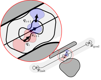
Figure 3: Visualization of the proof of completeness. $\boldsymbol{s}_{i+1}$ is placed along the (unknown) path of maximum clearance $\sigma$ such that $\boldsymbol{q}_{i}$ lies on the border of $\mathcal{R}_{\mathrm{dist}}(\boldsymbol{s}_{i+1},\tilde{d}_{\mathrm{dist}})$. Since $\mathcal{R}_{\mathrm{dist}}(\boldsymbol{q}_{i},\tilde{d}_{\mathrm{dist}})$ and $\mathcal{R}_{\mathrm{dist}}(\boldsymbol{q}_{i+1},\tilde{d}_{\mathrm{dist}})$ overlap and are fully contained in $\mathcal{R}_{\mathrm{dist}}(\boldsymbol{s}_{i+1},2\tilde{d}_{\mathrm{dist}})$ the path from $\boldsymbol{q}_{i}$ to $\boldsymbol{q}_{i+1}$ is collision free.

III-D1 Completeness

We show that the approach deterministically returns a solution if it exists and returns failure otherwise [8, 3, 19]. Note that this is a stronger property than probabilistic completeness [7].

Theorem 1

Given a set of samples $\mathcal{S}$ with known dispersion $\tilde{d}_{\mathrm{dist}}$ and considering general driftless systems for which we have steer functions that are optimal and symmetric, we can solve all planning queries $\gamma$ with Alg. 1 using a connection radius $r>2\tilde{d}_{\mathrm{dist}}$ having clearance of

$$\delta_{\mathrm{dist}}(\gamma)>2\tilde{d}_{\mathrm{dist}}.$$ (7)

Proof:

To see this, first note that $\mathcal{R}_{\mathrm{dist}}(\boldsymbol{x},r)$ for optimal steering functions, is equivalent to time-limited reachable sets of the system. Hence, trajectories from $\boldsymbol{x}$ to any other point in $\mathcal{R}_{\mathrm{dist}}(\boldsymbol{x},r)$ will also be fully contained in $\mathcal{R}_{\mathrm{dist}}(\boldsymbol{x},r)$. Given a query $\gamma$ with clearance $\delta(\gamma)>2\tilde{d}_{\mathrm{dist}}$, there exists a solution $\sigma$ with $\mathcal{R}(\boldsymbol{s}_{i},2\tilde{d}_{\mathrm{dist}})\in\mathcal{X}_{\mathrm{free}},~{}\forall\boldsymbol{s}_{i}\in\sigma^{*}$. First note that due to the dispersion definition, there must be a sample of $\mathcal{S}$ in both $\mathcal{R}_{\mathrm{dist}}(\boldsymbol{x}_{\mathrm{start}},\tilde{d}_{\mathrm{dist}})$ and $\mathcal{R}_{\mathrm{dist}}(\boldsymbol{x}_{\mathrm{goal}},\tilde{d}_{\mathrm{dist}})$. Thus it is possible to connect the start and goal configuration to the roadmap. It remains to show that a $\mathrm{dist}$-clearance of $\delta_{\mathrm{dist}}(\gamma)>2\tilde{d}_{\mathrm{dist}}$ is sufficient to find a path from $\boldsymbol{x}_{\mathrm{start}}$ to $\boldsymbol{x}_{\mathrm{goal}}$. Let $\boldsymbol{q}_{0}$ and $\boldsymbol{q}_{N}$ denote the samples that $\boldsymbol{x}_{\mathrm{start}}$ and $\boldsymbol{x}_{\mathrm{goal}}$ are connected to, respectively. By taking $\boldsymbol{s}_{1}$ along a path $\sigma$ and such that $\boldsymbol{q}_{0}$ lies on the border of $\mathcal{R}_{\mathrm{dist}}(\boldsymbol{s}_{1},\tilde{d}_{\mathrm{dist}})$ we see, due to the dispersion definition in Eq. 6, that there must be another sample in the reachable set, denoted by $\boldsymbol{q}_{1}$. At this point we only know that the path from $\boldsymbol{q}_{0}$ over $\boldsymbol{s}_{1}$ to $\boldsymbol{q}_{1}$ must be collision free. Since only $\boldsymbol{q}_{0}$ and $\boldsymbol{q}_{1}$ are known, we require a factor of 2 in the clearance (i.e., $2\tilde{d}_{\mathrm{dist}}$ in Eq. 7), which ensures that the path from $\boldsymbol{q}_{0}$ to $\boldsymbol{q}_{1}$ must be collision-free. To see this, note that due the system symmetry both $\mathcal{R}_{\mathrm{dist}}(\boldsymbol{q}_{\mathrm{0}},\tilde{d}_{\mathrm{dist}})$ and $\mathcal{R}_{\mathrm{dist}}(\boldsymbol{q}_{\mathrm{1}},\tilde{d}_{\mathrm{dist}})$ must be contained in $\mathcal{R}(\boldsymbol{s}_{1},2\tilde{d}_{\mathrm{dist}})\subset\mathcal{X}_{\mathrm{free}}$. We also know that the intersection $\mathcal{R}_{\mathrm{dist}}(\boldsymbol{q}_{\mathrm{0}},\tilde{d}_{\mathrm{dist}})\cap\mathcal{R}_{\mathrm{dist}}(\boldsymbol{q}_{\mathrm{1}},\tilde{d}_{\mathrm{dist}})$ contains $\boldsymbol{s}_{1}$ and is thus nonempty. The trajectory from $\boldsymbol{q}_{0}$ to $\boldsymbol{q}_{1}$ must pass through this intersection and is hence collision-free. The same idea can now be repeated until the path to $\boldsymbol{q}_{N}$ is found. Fig. 3 visualizes the proof. ∎

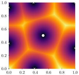
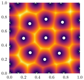
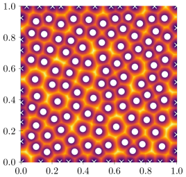
Figure 4: Progression of the algorithm in 2D Euclidean space. The background color indicates the distance to the next sample (i.e., the distance matrix $\boldsymbol{D}$). The white crosses and dots show the processed border points and actual samples respectively.

III-D2 Asymptotic Optimality

In this section, following [3] we will show that PRM* is asymptotically optimal when using the sampling sets generated by Dispertio. Particularly, Janson et al. [3] show that PRM* is asymptotically optimal when using deterministic sampling sets in $D$ dimensions whose dispersion is upper-bounded by $\gamma~{}n^{-1/D},~{}\gamma>0$. Next, we will show how the sampling sets generated by our approach reach the same asymptotic dispersion (see Theorem 2), i.e., lower $l_{2}$-dispersions, for all driftless control-affine systems, therefore retaining the PRM* asymptotic optimality. For the special Euclidean case, we show that the algorithm reaches the same asymptotically optimal dispersion as for example the Halton sequence. Note that for simplicity we are using a simplified version of the algorithm, without discretization and assuming the distance to the border is known. Throughout the discussion we again assume that the distance function $\mathrm{dist}$ is symmetric and optimal. Also note that $\mathcal{R}(\boldsymbol{x},r)$ now denotes the open ball of radius $r$ at $\boldsymbol{x}$ and $V(\cdot)$ the volume of a set.

Theorem 2

Under the assumption that the discretization of the space does not influence the placement of the samples, Alg. 2 dispersion can be bounded by

$$nV(\mathcal{R}(\boldsymbol{x},d_{n}/2))\leq V(\mathcal{X})$$ (8)

where $d_{n}$ denotes the dispersion defined for a distance function $\mathrm{dist}$ as in Eq. 5, when $n$ samples have been picked, i.e., $|\mathcal{S}|=n$. This yields for the $D$-dimensional Euclidean case an asymptotic behavior of

$$d_{n}\in\mathcal{O}\left(n^{-1/D}\right)$$ (9)

and the driftless control-affine case

$$d_{n}\in\mathcal{O}\left(n^{-1/\tilde{D}}\right)$$ (10)

with $\tilde{D}=\sum_{i=1}^{D}w_{i}$, where $w_{i}$ are the weights of the boxes approximating the reachability space for driftless control-affine systems (see ball-box theorem [12, 2]).

Proof:

To prove the asymptotic behavior of the algorithm, let us consider the case in which the discretization of the space has no effect on the placement of samples. The key argument to analyze the asymptotic behavior of the algorithm is to realize that the $n$th sample is, by construction, placed such that its distance to the closest neighbor is $d_{n-1}$. Due to that, after $n$ samples have been picked, we can note that

$$d_{n-1}\leq\min_{\boldsymbol{y}\in\mathcal{S}\setminus\boldsymbol{x}}\mathrm{dist}(\boldsymbol{x},\boldsymbol{y})\leq 2d_{n-1}\quad\forall\boldsymbol{x}\in\mathcal{S},$$ (11)

where the second inequality follows from the symmetry and optimality assumption of $\mathrm{dist}$. From the first inequality it follows that (note that the ball is open)

$$\mathcal{R}(\boldsymbol{x},d_{n-1})\cap\mathcal{S}=\emptyset\quad\forall\boldsymbol{x}\in\mathcal{S}.$$ (12)

In addition, because of symmetry and optimality, the intersection of all open balls of radius $d_{n-1}/2$ must be empty, i.e.,

$$\bigcap\limits_{\boldsymbol{x}\in\mathcal{S}}\mathcal{R}(\boldsymbol{x},d_{n-1}/2)=\emptyset.$$ (13)

Note that $d_{n}\leq d_{n-1}$ and with $n$ samples being in $\mathcal{S}$ we can state that

$$nV\big{(}\mathcal{R}(\boldsymbol{x},d_{n}/2)\big{)}\leq V(\mathcal{X})$$ (14)

must hold. To upper bound the dispersion for a number of samples $n$ we would optimally use an explicit term for the volume $V\big{(}\mathcal{R}(\boldsymbol{x},d_{n}/2)\big{)}$, but if no such term exists (as for general sub-Riemannian balls), we need to use a lower bound, for example by using the ball-box theorem. Let us first consider the case of a $D$-dimensional Euclidean space $\mathcal{X}$. In that case we obtain

$$n\alpha d_{n}^{D}\leq V(\mathcal{X})$$ (15)

and thus

$$d_{n}\leq\frac{V(\mathcal{X})^{1/D}}{\alpha^{1/D}n^{1/D}}\in\mathcal{O}\left(n^{-1/D}\right)$$ (16)

with $\alpha>0$. This shows that in the Euclidean case, the achieved asymptotic dispersion is the same as for $l_{2}$ low dispersion sequences (e.g., Halton). For the driftless control-affine case we can use the same argumentation as in [19]. Under the assumption that the system is sufficiently regular we can find a parameter $A_{\mathrm{max}}$ such that

$$\mathrm{Box}^{w}\left(\boldsymbol{x},\frac{d_{n}}{2A_{\mathrm{max}}}\right)\subseteq\mathcal{R}(\boldsymbol{x},d_{n}/2)$$ (17)

and according to Lemma II.2 by Schmerling et al. [21] the volume is given by

$$V\Bigg{(}\mathrm{Box}^{w}\left(\boldsymbol{x},\frac{d_{n}}{2A_{\mathrm{max}}}\right)\Bigg{)}=\left(\frac{d_{n}}{2A_{\mathrm{max}}}\right)^{\tilde{D}}$$ (18)

with $\tilde{D}=\sum_{i=1}^{D}w_{i}$. We can rewrite Eq. 14 as

$$n\left(\frac{d_{n}}{2A_{\mathrm{max}}}\right)^{\tilde{D}}\leq V(\mathcal{X})$$ (19)

and thus

$$d_{n}\leq\frac{V(\mathcal{X})^{1/\tilde{D}}2A_{\mathrm{max}}}{n^{1/\tilde{D}}}\in\mathcal{O}\left(n^{-1/\tilde{D}}\right).$$ (20)

∎

Note that if the number of samples approaches the discretization of the space, they will actually converge to a Sukharev grid [24]. Hence, in the Euclidean case, the asymptotic dispersion is still $\mathcal{O}\left(n^{-1/D}\right)$, but in the general case, we would need to inner-bound the reachable set with a Euclidean ball, which would lead to rather crude approximations as shown by Janson et al. [3] for the linear affine case. Thus, especially for nonholonomic systems, a grid of high resolution may be important to capture the shape of the reachable sets. Fig. 5 numerically compares the dispersion for the Reeds-Shepp case after $n$ samples for i.i.d., Halton and the proposed approach.

Given that our set $S$ has the same asymptotic dispersion as $l_{2}$ low dispersion sequences, our approach retains the asymptotic analysis carried out in [3, 19] and it allows the usage of a PRM* connection radius $r_{n}\in\omega(n^{-1/D})$.

IV Evaluation

In this section we describe the experiments to evaluate how our approach performs in terms of planning efficiency and path quality compared to a set of baselines.

To this end, we design two main experiments. In the first experiment, we compare our approach against the baselines (uniform i.i.d. samples, Halton samples [8], Poccia’s approach [19], state-lattice approach [18]) for a car-like kinematic systems (i.e., Reeds-Shepp (RS) [20]), over a subset of maps from the benchmark moving-ai [22], i.e., city maps, see Fig. 7 for example maps. The benchmark contains maps with several narrow corridors, and the planner needs to perform complex maneuvers (i.e., fully exploiting the full maneuverability), to let the car achieve its goal. We use a minimum turning radius $\rho=5\textrm{~{}m}$ and plan in environments of different size with $w$ being the width of the map. For the state lattice, sets of motion primitives have been chosen after an informal validation and are shown in Fig. 6. The actual dispersion is reported as $\tilde{d}_{\mathrm{rs}}$ and the number of drawn samples as $n_{\mathrm{all}}$.

In the second experiment, we compare the approach to the baselines on a set of randomized maps and random planning queries. To show the general applicability of the algorithm we also benchmark it for a 6D kinematic chain in the 2D plane (comparing it to Halton sequence and i.i.d. samples). In this case, each joint either has an angle $\theta_{i}\in[-3,3]$ with $i=1,...,6$, or we plan in an identified space (i.e., the arms can wrap around) with $\theta_{i}\in[-\pi,\pi]/\sim$. We use as distance function the 2-norm in joint space (respecting the possible identification).

In both experiments we evaluate the approach in terms of cost (i.e., path length) and success rate, and show planning efficiency by plotting the cost progression. Additionally we compare the trend for the dispersion (Eq. 6) conditioned on the number of samples for the car-like kinematics, obtained by our approach and the different baselines, see Fig. 5.

We use OMPL [23] and adopt its PRM* implementation (we made it deterministic by removing the random walk expansion step), with the default $k$-nearest connection strategy of $k_{n}=e\left(1+1/D\right)\log n$, which ensures asymptotic optimality for all the samplers. The same nearest neighborhood search and collision checkers (only different for examined systems) are used for all experiments and they are run on a machine with Xeon E5-1620 CPU and 32GB of RAM.

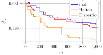
Figure 5: Dispersion trend for the Reeds-Shepp case ($\eta=1.0$, obstacle free environment). Our approach obtains a better dispersion than the baselines, thus achieving a better coverage of the state space as also shown in Fig. 1.

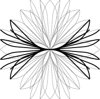
(a) $2\,\mathrm{m}$ grid

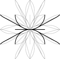
(b) $5\,\mathrm{m}$ grid

Figure 6: The motion primitive sets, used for the state lattice approaches in Table I(a) and I(b), respectively.

V Results and Discussion

We collect the evaluation’s results in Tables I-II. The tables’ scores report how often an approach (on the table row) generates a better solution than another (on the table column). Whenever an approach is better, the score was changed by $+1$, by $0$ for a draw (i.e., both fail to find a solution), and $-1$ if the approach yielded the higher cost. Results are shown for different ratios $\eta=\rho/w$. In Table I, a green cell highlights that the approach on the table row has a better performance of the one indicated on the table column, red otherwise. Table II reports only the scores obtained by Dispertio against the baselines.

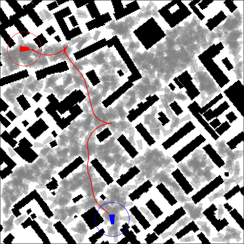
(a) i.i.d.

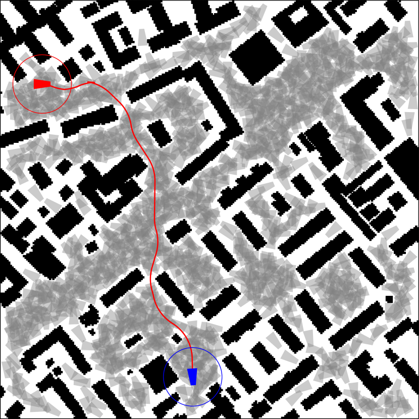
(b) Halton

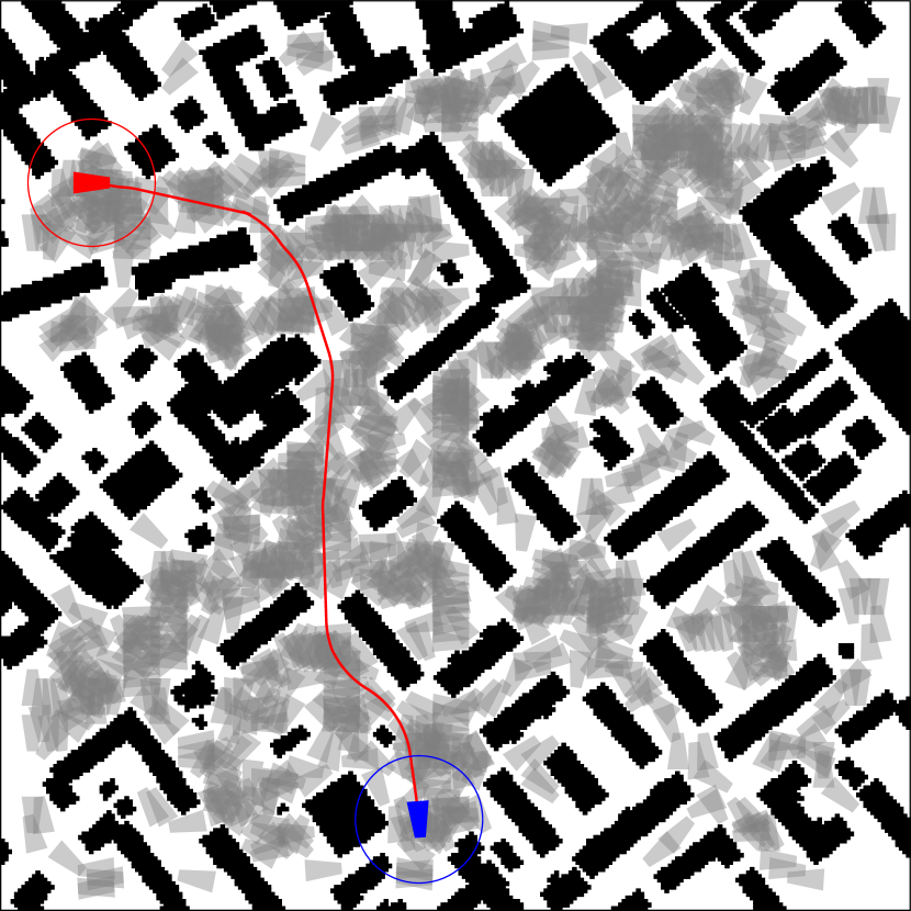
(c) Dispertio

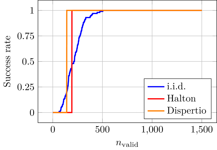
(d) Success rate

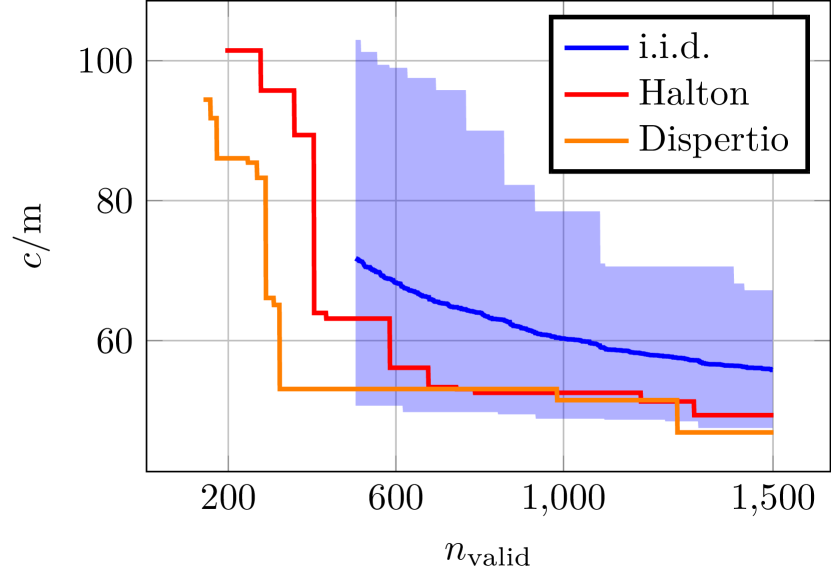
(e) Cost

Figure 7: Qualitative comparison of i.i.d., Halton and Dispertio. The top row shows example paths obtained after $1500$ valid samples connecting starts (in red) with goals (in blue). The gray footprints represent the roadmap’s vertices. The bottom row shows success rate and cost for this example.

Experiment 1) Table I shows the results of the first experiment considering 13 maps with 50 queries each (i.e., a total of 650 planning queries, thus results have been normalized with $\sigma_{\mathrm{rand}}=\sqrt{650}$). Overall our approach achieves better costs and a higher success rate compared to the baselines. In general, Halton is the second best placed. State-lattice performs poorly, indicating that more effort is required for their motion primitives design (i.e., possibly also using a notion of dispersion in control space). Fig. 7 shows an example planning query for i.i.d., Halton sampling and our approach. It reports the obtained paths, the trend for the success rate and the cost progression. The blue range shows the minimum and maximum cost observed in these runs for the i.i.d. sampler. The cost results are only shown for success rates of $100\%$. Cost and success rate progressions of Fig. 7 show how our approach is faster in getting an initial good solution, and faster (as the number of samples increases) in converging to lower cost solutions in those cluttered and narrow scenarios.

Experiment 2)  Table II shows the results for the second experiment. They are normalized by $\sigma_{\mathrm{rand}}=\sqrt{1000}$, with 1000 being the the amount of random planning queries. Also for the second experiment, our approach achieves better performance in terms of final cost solution even in higher dimensional spaces. Furthermore, in very cluttered environments (with $\eta=1.0$) our approach achieves on average a 10% higher success rate than the baselines, indicating how it can better exploit the knowledge of the nonholonomic constraints (i.e., maneuvering capabilities) in narrower scenarios.

Moreover as reported in Fig. 5, Dispertio has a lower dispersion value at each iteration (i.e., numbers of samples) than the baselines, mainly due to the fact that it better exploits the knowledge of the system dynamics (i.e., by using the steer function and the reachable set computation).

	i.i.d.	Halton	Poccia	Dispertio	Lattice
i.i.d.	$\cdot$	-3.41	-3.06	-5.33	21.93
Halton	3.41	$\cdot$	-0.08	-1.26	22.28
Poccia	3.06	0.078	$\cdot$	-1.06	21.53
Dispertio	5.33	1.26	1.06	$\cdot$	22.75
Lattice	-21.93	-22.28	-21.53	-22.75	$\cdot$

(a) PRM*, Reeds-Shepp, $\eta=0.1$, $n_{\mathrm{all}}=5000$

	i.i.d.	Halton	Poccia	Dispertio	Lattice
i.i.d.	$\cdot$	-4.79	-4.04	-9.18	21.69
Halton	4.79	$\cdot$	1.26	-4.31	23.3
Poccia	4.04	-1.26	$\cdot$	-4.98	23.06
Dispertio	9.18	4.31	4.98	$\cdot$	23.65
Lattice	-21.69	-23.3	-23.06	-23.65	$\cdot$

(b) PRM*, Reeds-Shepp, $\eta=0.05$, $n_{\mathrm{all}}=3200$

TABLE I: Path quality results of all the methods for the city-maps benchmark [22]. Dispertio obtains on average better solutions against all the baselines.

	i.i.d.	Halton	Poccia
RS, $\eta=1$, $n_{\mathrm{all}}=1500$	4.87	4.11	3.1
RS, $\eta=0.25$, $n_{\mathrm{all}}=1500$	6.26	4.08	1.20
RS, $\eta=0.1$, $n_{\mathrm{all}}=1500$	10.69	6.7	2.47
RS, $\eta=0.05$, $n_{\mathrm{all}}=1500$	11.61	7.15	4.59
KC, $\{[-\pi,\pi]/\sim\}^{6}$, $n_{\mathrm{all}}=30000$	2.28	1.01	$\cdot$
KC, $[-3,3]^{6}$, $n_{\mathrm{all}}=30000$	7.78	7.78	$\cdot$

TABLE II: Path quality performance of Dispertio against the baselines, on randomized maps and queries in different spaces (Reed-Shepp and 6D Kinematic Chain).

VI Conclusions

In this work we extend deterministic sampling-based motion planning to the class of symmetric and optimal driftless systems, by proposing Dispertio, an algorithm for optimized deterministic sampling set generation. When used in combination with PRM*, we prove that the approach is deterministically complete and retains asymptotic optimality. In the evaluation, we show that our sampling technique outperforms state-of-the-art methods in terms of solution cost and planning efficiency, while also converging faster to lower cost solutions. As future work, we are interested in extending the approach towards non-uniform sampling schemes, for example to exploit learned priors, and to systems with drift.

References

- [1] Michael S Branicky, Steven M LaValle, Kari Olson, and Libo Yang. Quasi-randomized path planning. In Int. Conf. on Robotics and Automation (ICRA), Seoul, Korea, 2001.
- [2] Wei-Liang Chow. Über systeme von linearen partiellen differential-gleichungen erster ordnung. In The Collected Papers Of Wei-Liang Chow. World Scientific, 2002.
- [3] Lucas Janson, Brian Ichter, and Marco Pavone. Deterministic sampling-based motion planning: Optimality, complexity, and performance. Int. Journal of Robotics Research, 37(1), 2018.
- [4] Lucas Janson, Edward Schmerling, Ashley Clark, and Marco Pavone. Fast marching tree: A fast marching sampling-based method for optimal motion planning in many dimensions. Int. Journal of Robotics Research, 34(7), 2015.
- [5] Sertac Karaman and Emilio Frazzoli. Sampling-based algorithms for optimal motion planning. Int. Journal of Robotics Research, 30(7), 2011.
- [6] LE Kavraki, P Svestka, J-C Latombe, and MH Overmars. Probabilistic roadmaps for path planning in high-dimensional configuration spaces. IEEE Transactions on Robotics and Automation, 12(4), 1996.
- [7] Steven M LaValle. Planning algorithms. Cambridge university press, 2006.
- [8] Steven M LaValle, Michael S Branicky, and Stephen R Lindemann. On the relationship between classical grid search and probabilistic roadmaps. Int. Journal of Robotics Research, 23(7-8), 2004.
- [9] Steven M LaValle and James J Kuffner Jr. Randomized kinodynamic planning. Int. Journal of Robotics Research, 20(5), 2001.
- [10] Jed Lengyel, Mark Reichert, Bruce R Donald, and Donald P Greenberg. Real-time robot motion planning using rasterizing computer graphics hardware, volume 24. ACM, 1990.
- [11] Tomás Lozano-Pérez and Michael A Wesley. An algorithm for planning collision-free paths among polyhedral obstacles. Communications of the ACM, 22(10), 1979.
- [12] Richard Montgomery. A tour of subriemannian geometries, their geodesics and applications. American Mathematical Soc., 2002.
- [13] Alex Nash, Kenny Daniel, Sven Koenig, and Ariel Felner. Theta*: Any-angle path planning on grids. In AAAI, volume 7, 2007.
- [14] Harald Niederreiter. Random number generation and quasi-Monte Carlo methods, volume 63. Siam, 1992.
- [15] Luigi Palmieri and Kai O Arras. A novel RRT extend function for efficient and smooth mobile robot motion planning. In Int. Conf. on Intelligent Robots and Systems (IROS), Chicago, USA, 2014.
- [16] Luigi Palmieri, Sven Koenig, and Kai O Arras. RRT-based nonholonomic motion planning using any-angle path biasing. In Int. Conf. on Robotics and Automation (ICRA), Stockholm, Sweden, 2016.
- [17] Luigi Palmieri, Tomasz P Kucner, Martin Magnusson, Achim J Lilienthal, and Kai O Arras. Kinodynamic motion planning on gaussian mixture fields. In Int. Conf. on Robotics and Automation (ICRA), Singapore, 2017.
- [18] Mihail Pivtoraiko and Alonzo Kelly. Kinodynamic motion planning with state lattice motion primitives. In Int. Conf. on Intelligent Robots and Systems (IROS), San Francisco, USA, 2011.
- [19] Ernesto Poccia. Deterministic sampling-based algorithms for motion planning under differential constraints. Master’s thesis, Stanford University, 2017.
- [20] James Reeds and Lawrence Shepp. Optimal paths for a car that goes both forwards and backwards. Pacific journal of mathematics, 145(2), 1990.
- [21] Edward Schmerling, Lucas Janson, and Marco Pavone. Optimal sampling-based motion planning under differential constraints: the driftless case. In Int. Conf. on Robotics and Automation (ICRA), 2015.
- [22] N. Sturtevant. Benchmarks for grid-based pathfinding. Transactions on Computational Intelligence and AI in Games, 4(2), 2012.
- [23] Ioan A Sucan, Mark Moll, and Lydia E Kavraki. The open motion planning library. IEEE Robotics & Automation Magazine, 19(4), 2012.
- [24] Aleksandr G Sukharev. Optimal strategies of the search for an extremum. USSR Computational Mathematics and Mathematical Physics, 11(4), 1971.
- [25] Johannes van der Corput. Verteilungsfunktionen i & ii. In Nederl. Akad. Wetensch. Proc., volume 38, 1935.