A New Framework for Distance and Kernel-based Metrics in High Dimensions

Abstract

The paper presents new metrics to quantify and test for (i) the equality of distributions and (ii) the independence between two high-dimensional random vectors. We show that the energy distance based on the usual Euclidean distance cannot completely characterize the homogeneity of two high-dimensional distributions in the sense that it only detects the equality of means and the traces of covariance matrices in the high-dimensional setup. We propose a new class of metrics which inherits the desirable properties of the energy distance and maximum mean discrepancy/(generalized) distance covariance and the Hilbert-Schmidt Independence Criterion in the low-dimensional setting and is capable of detecting the homogeneity of/completely characterizing independence between the low-dimensional marginal distributions in the high dimensional setup. We further propose t-tests based on the new metrics to perform high-dimensional two-sample testing/independence testing and study their asymptotic behavior under both high dimension low sample size (HDLSS) and high dimension medium sample size (HDMSS) setups. The computational complexity of the t-tests only grows linearly with the dimension and thus is scalable to very high dimensional data. We demonstrate the superior power behavior of the proposed tests for homogeneity of distributions and independence via both simulated and real datasets.

Keywords: Distance Covariance, Energy Distance, High Dimensionality, Hilbert-Schmidt Independence Criterion, Independence Test, Maximum Mean Discrepency, Two Sample Test, U-statistic.

1 Introduction

Nonparametric two-sample testing of homogeneity of distributions has been a classical problem in statistics, finding a plethora of applications in goodness-of-fit testing, clustering, change-point detection and so on. Some of the most traditional tools in this domain are Kolmogorov-Smirnov test, and Wald-Wolfowitz runs test, whose multivariate and multidimensional extensions have been studied by Darling (1957), David (1958) and Bickel (1969) among others. Friedman and Rafsky (1979) proposed a distribution-free multivariate generalization of the Wald-Wolfowitz runs test applicable for arbitrary but fixed dimensions. Schilling (1986) proposed another distribution-free test for multivariate two-sample problem based on $k$-nearest neighbor ($k$-NN) graphs. Maa et al. (1996) suggested a technique for reducing the dimensionality by examining the distribution of interpoint distances. In a recent novel work, Chen and Friedman (2017) proposed graph-based tests for moderate to high dimensional data and non-Euclidean data. The last two decades have seen an abundance of literature on distance and kernel-based tests for equality of distributions. Energy distance (first introduced by Székely (2002)) and maximum mean discrepancy or MMD (see Gretton et al. (2012)) have been widely studied in both the statistics and machine learning communities. Sejdinovic et al. (2013) provided a unifying framework establishing the equivalence between the (generalized) energy distance and MMD. Although there have been some very recent works to gain insight on the decaying power of the distance and kernel-based tests for high dimensional inference (see for example Ramdas et al. (2015a, 2015b), Kim et al. (2018) and Li (2018)), the behavior of these tests in the high dimensional setup is still a pretty unexplored area.

Measuring and testing for independence between two random vectors has been another fundamental problem in statistics, which has found applications in a wide variety of areas such as independent component analysis, feature selection, graphical modeling, causal inference, etc. There has been an enormous amount of literature on developing dependence metrics to quantify non-linear and non-monotone dependence in the low dimensional context. Gretton et al. (2005, 2007) introduced a kernel-based independence measure, namely the Hilbert-Schmidt Independence Criterion (HSIC). Bergsma and Dassios (2014) proposed a consistent test of independence of two ordinal random variables based on an extension of Kendall’s tau. Josse and Holmes (2014) suggested tests of independence based on the RV coefficient. Székely et al. (2007), in their seminal paper, introduced distance covariance (dCov) to characterize dependence between two random vectors of arbitrary dimensions. Lyons (2013) extended the notion of distance covariance from Euclidean spaces to arbitrary metric spaces. Sejdinovic et al. (2013) established the equivalence between HSIC and (generalized) distance covariance via the correspondence between positive definite kernels and semi-metrics of negative type. Over the last decade, the idea of distance covariance has been widely extended and analyzed in various ways; see for example Zhou (2012), Székely and Rizzo (2014), Wang et al. (2015), Shao and Zhang (2014), Huo and Székely (2016), Zhang et al. (2018), Edelmann et al. (2018) among many others. There have been some very recent literature which aims at generalizing distance covariance to quantify the joint dependence among more than two random vectors; see for example Matteson and Tsay (2017), Jin and Matteson (2017), Chakraborty and Zhang (2018), Böttcher (2017), Yao et al. (2018), etc. However, in the high dimensional setup, the literature is scarce, and the behavior of the widely used distance and kernel-based dependence metrics is not very well explored till date. Székely and Rizzo (2013) proposed a distance correlation based t-test to test for independence in high dimensions. In a very recent work, Zhu et al. (2018) showed that in the high dimension low sample size (HDLSS) setting, i.e., when the dimensions grow while the sample size is held fixed, the sample distance covariance can only measure the component-wise linear dependence between the two vectors. As a consequence, the distance correlation based t-test proposed by Székely et al. (2013) for independence between two high dimensional random vectors has trivial power when the two random vectors are nonlinearly dependent but component-wise uncorrelated. As a remedy, Zhu et al. (2018) proposed a test by aggregating the pairwise squared sample distance covariances and studied its asymptotic behavior under the HDLSS setup.

This paper presents a new class of metrics to quantify the homogeneity of distributions and independence between two high-dimensional random vectors. The core of our methodology is a new way of defining the distance between sample points (interpoint distance) in the high-dimensional Euclidean spaces. In the first part of this work, we show that the energy distance based on the usual Euclidean distance cannot completely characterize the homogeneity of two high-dimensional distributions in the sense that it only detects the equality of means and the traces of covariance matrices in the high-dimensional setup. To overcome such a limitation, we propose a new class of metrics based on the new distance which inherits the nice properties of energy distance and maximum mean discrepancy in the low-dimensional setting and is capable of detecting the pairwise homogeneity of the low-dimensional marginal distributions in the HDLSS setup. We construct a high-dimensional two sample t-test based on the U-statistic type estimator of the proposed metric, which can be viewed as a generalization of the classical two-sample t-test with equal variances. We show under the HDLSS setting that the new two sample t-test converges to a central t-distribution under the null and it has nontrivial power for a broader class of alternatives compared to the energy distance. We further show that the two sample t-test converges to a standard normal limit under the null when the dimension and sample size both grow to infinity with the dimension growing more rapidly. It is worth mentioning that we develop an approach to unify the analysis for the usual energy distance and the proposed metrics. Compared to existing works, we make the following contribution.

• We derive the asymptotic variance of the generalized energy distance under the HDLSS setting and propose a computationally efficient variance estimator (whose computational cost is linear in the dimension). Our analysis is based on a pivotal t-statistic which does not require permutation or resampling-based inference and allows an asymptotic exact power analysis.

In the second part, we propose a new framework to construct dependence metrics to quantify the dependence between two high-dimensional random vectors $X$ and $Y$ of possibly different dimensions. The new metric, denoted by $\mathcal{D}^{2}(X,Y)$, generalizes both the distance covariance and HSIC. It completely characterizes independence between $X$ and $Y$ and inherits all other desirable properties of the distance covariance and HSIC for fixed dimensions. In the HDLSS setting, we show that the proposed population dependence metric behaves as an aggregation of group-wise (generalized) distance covariances. We construct an unbiased U-statistic type estimator of $\mathcal{D}^{2}(X,Y)$ and show that with growing dimensions, the unbiased estimator is asymptotically equivalent to the sum of group-wise squared sample (generalized) distance covariances. Thus it can quantify group-wise non-linear dependence between two high-dimensional random vectors, going beyond the scope of the distance covariance based on the usual Euclidean distance and HSIC which have been recently shown only to capture the componentwise linear dependence in high dimension, see Zhu et al. (2018). We further propose a t-test based on the new metrics to perform high-dimensional independence testing and study its asymptotic size and power behaviors under both the HDLSS and high dimension medium sample size (HDMSS) setups. In particular, under the HDLSS setting, we prove that the proposed t-test converges to a central t-distribution under the null and a noncentral t-distribution with a random noncentrality parameter under the alternative. Through extensive numerical studies, we demonstrate that the newly proposed t-test can capture group-wise nonlinear dependence which cannot be detected by the usual distance covariance and HSIC in the high dimensional regime. Compared to the marginal aggregation approach in Zhu et al. (2018), our new method enjoys two major advantages.

• Our approach provides a neater way of generalizing the notion of distance and kernel-based dependence metrics. The newly proposed metrics completely characterize dependence in the low-dimensional case and capture group-wise nonlinear dependence in the high-dimensional case. In this sense, our metric can detect a wider range of dependence compared to the marginal aggregation approach.

• The computational complexity of the t-tests only grows linearly with the dimension and thus is scalable to very high dimensional data.

Notation. Let $X=(X_{1},\dots X_{p})\in\mathbb{R}^{p}$ and $Y=(Y_{1},\dots,Y_{q})$ $\in\mathbb{R}^{q}$ be two random vectors of dimensions $p$ and $q$ respectively. Denote by $\|\cdot\|_{p}$ the Euclidean norm of $\mathbb{R}^{p}$ (we shall use it interchangeably with $\|\cdot\|$ when there is no confusion). Let $0_{p}$ be the origin of $\mathbb{R}^{p}$. We use $X\mathrel{\text{\scalebox{1.07}{$\perp\mkern-10.0mu\perp$}}}Y$ to denote that $X$ is independent of $Y$, and use $``X\overset{d}{=}Y"$ to indicate that $X$ and $Y$ are identically distributed. Let $(X^{\prime},Y^{\prime})$, $(X^{\prime\prime},Y^{\prime\prime})$ and $(X^{\prime\prime\prime},Y^{\prime\prime\prime})$ be independent copies of $(X,Y)$. We utilize the order in probability notations such as stochastic boundedness $O_{p}$ (big O in probability), convergence in probability $o_{p}$ (small o in probability) and equivalent order $\asymp$, which is defined as follows: for a sequence of random variables $\{Z_{n}\}_{n=1}^{\infty}$ and a sequence of real numbers $\{a_{n}\}_{n=1}^{\infty}$, $Z_{n}\asymp_{p}a_{n}$ if and only if $Z_{n}/a_{n}=O_{p}(1)$ and $a_{n}/Z_{n}=O_{p}(1)$ as $n\to\infty$. For a metric space $(\mathcal{X},d_{\mathcal{X}})$, let $\mathcal{M}(\mathcal{X})$ and $\mathcal{M}_{1}(\mathcal{X})$ denote the set of all finite signed Borel measures on $\mathcal{X}$ and all probability measures on $\mathcal{X}$, respectively. Define $\mathcal{M}^{1}_{d_{\mathcal{X}}}(\mathcal{X}):=\{v\in\mathcal{M}(\mathcal{X})\,:\,\exists\,x_{0}\in\mathcal{X}\;\text{s.t.}\;\int_{\mathcal{X}}d_{\mathcal{X}}(x,x_{0})\,d|v|(x)<\infty\}$. For $\theta>0$, define $\mathcal{M}_{\mathcal{K}}^{\theta}(\mathcal{X}):=\{v\in\mathcal{M}(\mathcal{X})\,:\,\int_{\mathcal{X}}\mathcal{K}^{\theta}(x,x)\,d|v|(x)<\infty\}$, where $\mathcal{K}:\mathcal{X}\times\mathcal{X}\to\mathbb{R}$ is a bivariate kernel function. Define $\mathcal{M}^{1}_{d_{\mathcal{Y}}}(\mathcal{Y})$ and $\mathcal{M}_{\mathcal{K}}^{\theta}(\mathcal{Y})$ in a similar way. For a matrix $A=(a_{kl})_{k,l=1}^{n}\in\mathbb{R}^{n\times n}$, define its $\mathcal{U}$-centered version $\tilde{A}=(\tilde{a}_{kl})\in\mathbb{R}^{n\times n}$ as follows

$$\tilde{a}_{kl}=\begin{cases}a_{kl}\,-\,{\frac{1}{n-2}}\displaystyle\sum_{j=1}^{n}a_{kj}\,-\,\frac{1}{n-2}\displaystyle\sum_{i=1}^{n}a_{il}\,+\,\frac{1}{(n-1)(n-2)}\displaystyle\sum_{i,j=1}^{n}a_{ij},\;&k\neq l,\\ 0,&k=l,\end{cases}$$ (1)

for $k,l=1,\dots,\,n$. Define

$$(\tilde{A}\cdot\tilde{B}):=\frac{1}{n(n-3)}\displaystyle\sum_{k\neq l}\tilde{a}_{kl}\tilde{b}_{kl}$$

for $\tilde{A}=(\tilde{a}_{kl})$ and $\tilde{B}=(\tilde{b}_{kl})\in\mathbb{R}^{n\times n}$. Denote by $\textrm{tr}(A)$ the trace of a square matrix $A$. $A\otimes B$ denotes the kronecker product of two matrices $A$ and $B$. Let $\Phi(\cdot)$ be the cumulative distribution function of the standard normal distribution. Denote by $t_{a,b}$ the noncentral t-distribution with $a$ degrees of freedom and noncentrality parameter $b$. Write $t_{a}=t_{a,0}$. Denote by $q_{\alpha,a}$ and $Z_{\alpha}$ the upper $\alpha$ quantile of the distribution of $t_{a}$ and the standard normal distribution, respectively, for $\alpha\in(0,1)$. Also denote by $\chi^{2}_{a}$ the chi-square distribution with $a$ degrees of freedom. Denote $U\sim$ Rademacher $(0.5)$  if  $P(U=1)=P(U=-1)=0.5$. Let $\mathbbm{1}_{A}$ denote the indicator function associated with a set $A$. Finally, denote by $\lfloor a\rfloor$ the integer part of $a\in\mathbb{R}$.

2 An overview: distance and kernel-based metrics

2.1 Energy distance and MMD

Energy distance (see Székely et al. (2004, 2005), Baringhaus and Franz (2004)) or the Euclidean energy distance between two random vectors $X,Y\in\mathbb{R}^{p}$ and $X\mathrel{\text{\scalebox{1.07}{$\perp\mkern-10.0mu\perp$}}}Y$ with $\mathbb{E}\|X\|_{p}<\infty$ and $\mathbb{E}\|Y\|_{p}<\infty$, is defined as

$$ED(X,Y)\;=\;2\,\mathbb{E}\|X-Y\|_{p}-\mathbb{E}\|X-X^{\prime}\|_{p}-\mathbb{E}\|Y-Y^{\prime}\|_{p}\;,$$ (2)

where $(X^{\prime},Y^{\prime})$ is an independent copy of $(X,Y)$. Theorem 1 in Székely et al. (2005) shows that  $ED(X,Y)\geq 0$ and the equality holds if and only if $X\overset{d}{=}Y$. In general, for an arbitrary metric space $(\mathcal{X},d)$, the generalized energy distance between $X\sim P_{X}$  and  $Y\sim P_{Y}$ where $P_{X},P_{Y}\in\mathcal{M}_{1}(\mathcal{X})\cap\mathcal{M}^{1}_{d}(\mathcal{X})$ is defined as

$$ED_{d}(X,Y)\;=\;2\,\mathbb{E}\,d(X,Y)-\mathbb{E}\,d(X,X^{\prime})-\mathbb{E}\,d(Y,Y^{\prime})\;.$$ (3)

Definition 2.1 (Spaces of negative type).

A metric space $(\mathcal{X},d)$ is said to have negative type if for all $n\geq 1$, $x_{1},\dots,x_{n}\in\mathcal{X}$ and $\alpha_{1},\dots,\alpha_{n}\in\mathbb{R}$  with $\sum_{i=1}^{n}\alpha_{i}=0$, we have

$$\sum_{i,j=1}^{n}\alpha_{i}\,\alpha_{j}\,d(x_{i},x_{j})\leq 0\;.$$ (4)

The metric space $(\mathcal{X},d)$ is said to be of strong negative type if the equality in (4) holds only when $\alpha_{i}=0$ for all $i\in\{1,\dots,n\}$.

If $(\mathcal{X},d)$ has strong negative type, then $ED_{d}(X,Y)$ completely characterizes the homogeneity of the distributions of $X$ and $Y$ (see Lyons (2013) and Sejdinovic et al. (2013) for detailed discussions). This quantification of homogeneity of distributions lends itself for reasonable use in one-sample goodness-of-fit testing and two sample testing for equality of distributions.

On the machine learning side, Gretton et al. (2012) proposed a kernel-based metric, namely maximum mean discrepancy (MMD), to conduct two-sample testing for equality of distributions. We provide some background before introducing MMD.

Definition 2.2.

(RKHS) Let $\mathcal{H}$ be a Hilbert space of real valued functions defined on some space $\mathcal{X}$. A bivariate function $\mathcal{K}:\mathcal{X}\times\mathcal{X}\to\mathbb{R}$ is called a reproducing kernel of $\mathcal{H}$ if :

1. $\forall x\in\mathcal{X},\mathcal{K}(\cdot,x)\in\mathcal{H}$

2. $\forall x\in\mathcal{X},\forall f\in\mathcal{H},\;\langle f,\mathcal{K}(\cdot,x)\rangle_{\mathcal{H}}=f(x)$

where $\langle\cdot,\cdot\rangle_{\mathcal{H}}$ is the inner product associated with $\mathcal{H}$. If $\mathcal{H}$ has a reproducing kernel, it is said to be a reproducing kernel Hilbert space (RKHS).

By Moore-Aronszajn theorem, for every positive definite function (also called a kernel) $\mathcal{K}:\mathcal{X}\times\mathcal{X}\to\mathbb{R}$, there is an associated RKHS $\mathcal{H}_{\mathcal{K}}$ with the reproducing kernel $\mathcal{K}$. The map $\Pi:\mathcal{M}_{1}(\mathcal{X})\to\mathcal{H}_{\mathcal{K}}$, defined as $\Pi(P)=\int_{\mathcal{X}}\mathcal{K}(\cdot,x)\,dP(x)$  for $P\in\mathcal{M}_{1}(\mathcal{X})$  is called the mean embedding function associated with $\mathcal{K}$. A kernel $\mathcal{K}$ is said to be characteristic to $\mathcal{M}_{1}(\mathcal{X})$ if the map $\Pi$ associated with $\mathcal{K}$ is injective. Suppose $\mathcal{K}$ is a characteristic kernel on $\mathcal{X}$. Then the MMD between $X\sim P_{X}$ and $Y\sim P_{Y}$, where $P_{X},P_{Y}\in\mathcal{M}_{1}(\mathcal{X})\cap\mathcal{M}^{1/2}_{\mathcal{K}}(\mathcal{X})$ is defined as

$$MMD_{\mathcal{K}}(X,Y)\; =\;\|\,\Pi(P_{X})\,-\,\Pi(P_{Y})\,\|_{\mathcal{H}_{\mathcal{K}}}\,.$$ (5)

By virtue of $\mathcal{K}$ being a characteristic kernel, $MMD_{\mathcal{K}}(X,Y)=0$  if and only if $X\overset{d}{=}Y$. Lemma 6 in Gretton et al. (2012) shows that the squared MMD can be equivalently expressed as

$$MMD^{2}_{\mathcal{K}}(X,Y)\;=\;\mathbb{E}\,\mathcal{K}(X,X^{\prime})\,+\,\mathbb{E}\,\mathcal{K}(Y,Y^{\prime})\,-\,2\,\mathbb{E}\,\mathcal{K}(X,Y)\;.$$ (6)

Theorem 22 in Sejdinovic et al. (2013) establishes the equivalence between (generalized) energy distance and MMD. Following is the definition of a kernel induced by a distance metric (refer to Section 4.1 in Sejdinovic et al. (2013) for more details).

Definition 2.3.

(Distance-induced kernel and kernel-induced distance) Let $(\mathcal{X},d)$ be a metric space of negative type and $x_{0}\in\mathcal{X}$. Denote $\mathcal{K}:\mathcal{X}\times\mathcal{X}\to\mathbb{R}$ as

$$\mathcal{K}(x,x^{\prime})\;=\;\frac{1}{2}\,\left\{d(x,x_{0})+d(x^{\prime},x_{0})-d(x,x^{\prime})\right\}.$$ (7)

The kernel $\mathcal{K}$ is positive definite if and only if $(\mathcal{X},d)$ has negative type, and thus $\mathcal{K}$ is a valid kernel on $\mathcal{X}$ whenever $d$ is a metric of negative type. The kernel $\mathcal{K}$ defined in (7) is said to be the distance-induced kernel induced by $d$ and centered at $x_{0}$. One the other hand, the distance $d$ can be generated by the kernel $\mathcal{K}$ through

$$d(x,x^{\prime})=\mathcal{K}(x,x)+\mathcal{K}(x^{\prime},x^{\prime})-2\mathcal{K}(x,x^{\prime}).$$ (8)

Proposition 29 in Sejdinovic et al. (2013) establishes that the distance-induced kernel $\mathcal{K}$ induced by $d$ is characteristic to $\mathcal{M}_{1}(\mathcal{X})\cap\mathcal{M}^{1}_{\mathcal{K}}(\mathcal{X})$ if and only if $(\mathcal{X},d)$ has strong negative type. Therefore, MMD can be viewed as a special case of the generalized energy distance in (3) with $d$ being the metric induced by a characteristic kernel.

Suppose $\{X_{i}\}^{n}_{i=1}$ and $\{Y_{i}\}^{m}_{i=1}$ are i.i.d samples of $X$ and $Y$ respectively. A U-statistic type estimator of $E_{d}(X,Y)$ is defined as

$$E_{n,m}(X,Y)=\frac{2}{nm}\sum_{k=1}^{n}\sum^{m}_{l=1}d(X_{k},Y_{l})-\frac{1}{n(n-1)}\sum_{k\neq l}^{n}d(X_{k},X_{l})-\frac{1}{m(m-1)}\sum_{k\neq l}^{m}d(Y_{k},Y_{l})\,.$$ (9)

In Section 4, we shall propose a new class of metrics for quantifying the homogeneity of high-dimensional distributions. This new class can be viewed as a particular case of the general measures in (3) with a suitably chosen distance $d$ to accommodate the high dimensionality. It thus inherits all the nice properties of $E_{d}(X,Y)$ in the low-dimensional context (see Proposition .1 and Theorem .2 in the supplementary material). With the specific choice of distance, the new metrics can detect a broader range of inhomogeneity between high-dimensional distributions compared to Euclidean energy distance.

2.2 Distance covariance and HSIC

Distance covariance (dCov) was first introduced in the seminal paper by Székely et al. (2007) to quantify the dependence between two random vectors of arbitrary (fixed) dimensions. Consider two random vectors $X\in\mathbb{R}^{p}$ and $Y\in\mathbb{R}^{q}$ with $\mathbb{E}\|X\|_{p}<\infty$ and $\mathbb{E}\|Y\|_{q}<\infty$. The Euclidean dCov between $X$ and $Y$ is defined as the positive square root of

$$dCov^{2}(X,Y)=\frac{1}{c_{p}c_{q}}\int_{{\mathbb{R}}^{p+q}}\frac{|f_{X,Y}(t,s)-f_{X}(t)f_{Y}(s)|^{2}}{\|t\|_{p}^{1+p}\,\|s\|_{q}^{1+q}}dtds,$$

where $f_{X}$, $f_{Y}$ and $f_{X,Y}$ are the individual and joint characteristic functions of $X$ and $Y$ respectively, and, $c_{p}=\pi^{(1+p)/2}/\,\Gamma((1+p)/2)$ is a constant with $\Gamma(\cdot)$ being the complete gamma function.

The key feature of dCov is that it completely characterizes independence between two random vectors of arbitrary dimensions, or in other words $dCov(X,Y)=0$ if and only if $X\mathrel{\text{\scalebox{1.07}{$\perp\mkern-10.0mu\perp$}}}Y$. According to Remark 3 in Székely et al. (2007), dCov can be equivalently expressed as

$$dCov^{2}(X,Y)\;=\;\mathbb{E}\,\|X-X^{\prime}\|_{p}\|Y-Y^{\prime}\|_{q}\,+\,\mathbb{E}\,\|X-X^{\prime}\|_{p}\,\mathbb{E}\,\|Y-Y^{\prime}\|_{q}\,-\,2\,\mathbb{E}\,\|X-X^{\prime}\|_{p}\|Y-Y^{\prime\prime}\|_{q}.\\$$ (10)

Lyons (2013) extends the notion of dCov from Euclidean spaces to general metric spaces. For arbitrary metric spaces $(\mathcal{X},d_{\mathcal{X}})$ and $(\mathcal{Y},d_{\mathcal{Y}})$, the generalized dCov between $X\sim P_{X}\in\mathcal{M}_{1}(\mathcal{X})\cap\mathcal{M}^{1}_{d_{\mathcal{X}}}(\mathcal{X})$  and  $Y\sim P_{Y}\in\mathcal{M}_{1}(\mathcal{Y})\cap\mathcal{M}^{1}_{d_{\mathcal{Y}}}(\mathcal{Y})$ is defined as

$$D^{2}_{d_{\mathcal{X}},d_{\mathcal{Y}}}(X,Y)\;=\;\mathbb{E}\,d_{\mathcal{X}}(X,X^{\prime})d_{\mathcal{Y}}(Y,Y^{\prime})\,+\,\mathbb{E}\,d_{\mathcal{X}}(X,X^{\prime})\,\mathbb{E}\,d_{\mathcal{Y}}(Y,Y^{\prime})\,-\,2\,\mathbb{E}\,d_{\mathcal{X}}(X,X^{\prime})d_{\mathcal{Y}}(Y,Y^{\prime\prime}).$$ (11)

Theorem 3.11 in Lyons (2013) shows that if $(\mathcal{X},d_{\mathcal{X}})$ and $(\mathcal{Y},d_{\mathcal{Y}})$ are both metric spaces of strong negative type, then $D_{d_{\mathcal{X}},d_{\mathcal{Y}}}(X,Y)=0$ if and only if $X\mathrel{\text{\scalebox{1.07}{$\perp\mkern-10.0mu\perp$}}}Y$. In other words, the complete characterization of independence by dCov holds true for any metric spaces of strong negative type. According to Theorem 3.16 in Lyons (2013), every separable Hilbert space is of strong negative type. As Euclidean spaces are separable Hilbert spaces, the characterization of independence by dCov between two random vectors in $(\mathbb{R}^{p},\|\cdot\|_{p})$ and $(\mathbb{R}^{q},\|\cdot\|_{q})$ is just a special case.

Hilbert-Schmidt Independence Criterion (HSIC) was introduced as a kernel-based independence measure by Gretton et al. (2005, 2007). Suppose $\mathcal{X}$ and $\mathcal{Y}$ are arbitrary topological spaces, $\mathcal{K}_{\mathcal{X}}$ and $\mathcal{K}_{\mathcal{Y}}$ are characteristic kernels on $\mathcal{X}$ and $\mathcal{Y}$ with the respective RKHSs $\mathcal{H}_{\mathcal{K}_{\mathcal{X}}}$ and $\mathcal{H}_{\mathcal{K}_{\mathcal{Y}}}$. Let $\mathcal{K}=\mathcal{K}_{\mathcal{X}}\otimes\mathcal{K}_{\mathcal{Y}}$ be the tensor product of the kernels $\mathcal{K}_{\mathcal{X}}$ and $\mathcal{K}_{\mathcal{Y}}$, and, $\mathcal{H}_{\mathcal{K}}$ be the tensor product of the RKHSs $\mathcal{H}_{\mathcal{K}_{\mathcal{X}}}$ and $\mathcal{H}_{\mathcal{K}_{\mathcal{Y}}}$. The HSIC between $X\sim P_{X}\in\mathcal{M}_{1}(\mathcal{X})\cap\mathcal{M}^{1/2}_{\mathcal{K}}(\mathcal{X})$  and  $Y\sim P_{Y}\in\mathcal{M}_{1}(\mathcal{Y})\cap\mathcal{M}^{1/2}_{\mathcal{K}}(\mathcal{Y})$ is defined as

$$HSIC_{\mathcal{K}_{\mathcal{X}},\mathcal{K}_{\mathcal{Y}}}(X,Y)\; =\;\|\,\Pi(P_{XY})\,-\,\Pi(P_{X}P_{Y})\,\|_{\mathcal{H}_{\mathcal{K}}},$$ (12)

where $P_{XY}$ denotes the joint probability distribution of $X$ and $Y$. The HSIC between $X$ and $Y$ is essentially the MMD between the joint distribution $P_{XY}$ and the product of the marginals $P_{X}$ and $P_{Y}$. Clearly, $HSIC_{\mathcal{K}_{\mathcal{X}},\mathcal{K}_{\mathcal{Y}}}(X,Y)=0$ if and only if $X\mathrel{\text{\scalebox{1.07}{$\perp\mkern-10.0mu\perp$}}}Y$. Gretton et al. (2005) shows that the squared HSIC can be equivalently expressed as

$$HSIC^{2}_{\mathcal{K}_{\mathcal{X}},\mathcal{K}_{\mathcal{Y}}}(X,Y)\; =\;\mathbb{E}\,\mathcal{K}_{\mathcal{X}}(X,X^{\prime})\mathcal{K}_{\mathcal{Y}}(Y,Y^{\prime})\,+\,\mathbb{E}\,\mathcal{K}_{\mathcal{X}}(X,X^{\prime})\,\mathbb{E}\,\mathcal{K}_{\mathcal{Y}}(Y,Y^{\prime})\,-\,2\,\mathbb{E}\,\mathcal{K}_{\mathcal{X}}(X,X^{\prime})\mathcal{K}_{\mathcal{Y}}(Y,Y^{\prime\prime}).$$ (13)

Theorem 24 in Sejdinovic et al. (2013) establishes the equivalence between the generalized dCov and HSIC.

For an observed random sample $(X_{i},Y_{i})^{n}_{i=1}$ from the joint distribution of $X$ and $Y$, a U-statistic type estimator of the generalized dCov in (11) can be defined as

$$\widetilde{D_{n}^{2}}_{\,;\,d_{\mathcal{X}},d_{\mathcal{Y}}}(X,Y)\;=\;(\tilde{A}\cdot\tilde{B})\;=\;\frac{1}{n(n-3)}\displaystyle\sum_{k\neq l}\tilde{a}_{kl}\tilde{b}_{kl}\;,$$ (14)

where $\tilde{A},\tilde{B}$ are the  $\mathcal{U}$-centered versions (see (1)) of $A=\big{(}d_{\mathcal{X}}(X_{k},X_{l})\big{)}_{k,l=1}^{n}$ and $B=\big{(}d_{\mathcal{Y}}(Y_{k},Y_{l})\big{)}_{k,l=1}^{n}$, respectively. We denote $\widetilde{D_{n}^{2}}_{\,;\,d_{\mathcal{X}},d_{\mathcal{Y}}}(X,Y)$ by $dCov^{2}_{n}(X,Y)$ when $d_{\mathcal{X}}$ and $d_{\mathcal{Y}}$ are Euclidean distances.

3 New distance for Euclidean space

We introduce a family of distances for Euclidean space, which shall play a central role in the subsequent developments. For $x\in\mathbb{R}^{\tilde{p}}$, we partition $x$ into $p$ sub-vectors or groups, namely $x=(x_{(1)},\dots,x_{(p)})$, where $x_{(i)}\in\mathbb{R}^{d_{i}}$ with $\sum_{i=1}^{p}d_{i}=\tilde{p}$. Let $\rho_{i}$ be a metric or semimetric (see for example Definition 1 in Sejdinovic et al. (2013)) defined on $\mathbb{R}^{d_{i}}$ for $1\leq i\leq p$. We define a family of distances for $\mathbb{R}^{\tilde{p}}$ as

$$K_{\bf{d}}(x,x^{\prime})\,:=\,\sqrt{\,\rho_{1}(x_{(1)},x_{(1)}^{\prime})\,+\,\dots\,+\,\rho_{p}(x_{(p)},x_{(p)}^{\prime})\,}\,,$$ (15)

where $x,x^{\prime}\in\mathbb{R}^{\tilde{p}}$ with $x=(x_{(1)},\dots,x_{(p)})$ and $x^{\prime}=(x^{\prime}_{(1)},\dots,x^{\prime}_{(p)})$, and $\textbf{d}=(d_{1},d_{2},\dots,d_{p})$ with $d_{i}\in\mathbb{Z}_{+}$ and $\sum_{i=1}^{p}d_{i}=\tilde{p}$.

Proposition 3.1.

Suppose each $\rho_{i}$ is a metric of strong negative type on $\mathbb{R}^{d_{i}}$. Then $\left(\mathbb{R}^{\tilde{p}},K_{\bf{d}}\right)$ satisfies the following two properties:

1. $K_{\bf{d}}:\mathbb{R}^{\tilde{p}}\times\mathbb{R}^{\tilde{p}}\rightarrow[0,\infty)$ is a valid metric on $\mathbb{R}^{\tilde{p}}$;

2. $\left(\mathbb{R}^{\tilde{p}},K_{\bf{d}}\right)$ has strong negative type.

In a special case, suppose  $\rho_{i}$  is the Euclidean distance on $\mathbb{R}^{d_{i}}$. By Theorem 3.16 in Lyons (2013), $(\mathbb{R}^{d_{i}},\rho_{i})$ is a separable Hilbert space, and hence has strong negative type. Then the Euclidean space equipped with the metric

$$K_{\bf{d}}(x,x^{\prime})\,=\,\sqrt{\,\|x_{(1)}-x_{(1)}^{\prime}\|\,+\,\dots\,+\,\|x_{(p)}-x_{(p)}^{\prime}\|\,}\,.$$ (16)

is of strong negative type. Further, if all the components $x_{(i)}$ are unidimensional, i.e., $d_{i}=1$ for $1\leq i\leq p$, then the metric boils down to

$$K_{\bf{d}}(x,x^{\prime})\;=\;\Arrowvert x-x^{\prime}\Arrowvert_{1}^{1/2}\;=\;\sqrt{\displaystyle\sum_{j=1}^{p}|x_{j}-x^{\prime}_{j}|}\;,$$ (17)

where $\Arrowvert x\Arrowvert_{1}=\sum_{j=1}^{p}|x_{j}|$  is the $l_{1}$ or the absolute norm on $\mathbb{R}^{p}$. If

$$\rho_{i}(x_{(i)},x_{(i)}^{\prime})=\|x_{(i)}-x_{(i)}^{\prime}\|^{2},\quad 1\leq i\leq p,$$ (18)

then $K_{\bf{d}}$ reduces to the usual Euclidean distance. We shall unify the analysis of our new metrics with the classical metrics by considering $K_{\bf{d}}$ which is defined in (15) with

1. each $\rho_{i}$ being a metric of strong negative type on $\mathbb{R}^{d_{i}}$;

2. each $\rho_{i}$ being a semimetric defined in (18).

The first case corresponds to the newly proposed metrics while the second case leads to the classical metrics based on the usual Euclidean distance. Remarks 3.1 and 3.2 provide two different ways of generalizing the class in (15). To be focused, our analysis below shall only concern about the distances defined in (15). In the numerical studies in Section 6, we consider $\rho_{i}$ to be the Euclidean distance and the distances induced by the Laplace and Gaussian kernels (see Definition 2.3) which are of strong negative type on $\mathbb{R}^{d_{i}}$ for $1\leq i\leq p$.

Remark 3.1.

A more general family of distances can be defined as

$$K_{\mathbf{d},r}(x,x^{\prime})=\Big{(}\rho_{1}(x_{(1)},x_{(1)}^{\prime})+\cdots+\rho_{p}(x_{(p)},x_{(p)}^{\prime})\Big{)}^{r},\quad 0<r<1.$$

According to Remark 3.19 of Lyons (2013), the space $(\mathbb{R}^{\tilde{p}},K_{\mathbf{d},r})$ is of strong negative type. The proposed distance is a special case with $r=1/2.$

Remark 3.2.

Based on the proposed distance, one can construct the generalized Gaussian and Laplacian kernels as

$$f(K_{\mathbf{d}}(x,x^{\prime})/\gamma)=\begin{cases}\exp(-K_{\mathbf{d}}^{2}(x,x^{\prime})/\gamma^{2}),\quad&f(x)=\exp(-x^{2})\text{ for Gaussian kernel},\\ \exp(-K_{\mathbf{d}}(x,x^{\prime})/\gamma),\quad&f(x)=\exp(-x)\text{ for Laplacian kernel}.\end{cases}$$

If $K_{\bf{d}}$ is translation invariant, then by Theorem 9 in Sriperumbudur et al. (2010) it can be verified that $f(K_{\mathbf{d}}(x,x^{\prime})/\gamma)$ is a characteristic kernel on $\mathbb{R}^{\tilde{p}}$. As a consequence, the Euclidean space equipped with the distance

$$K_{\mathbf{d},f}(x,x^{\prime})=f(K_{\mathbf{d}}(x,x)/\gamma)+f(K_{\mathbf{d}}(x^{\prime},x^{\prime})/\gamma)-2f(K_{\mathbf{d}}(x,x^{\prime})/\gamma)$$

is of strong negative type.

Remark 3.3.

In Sections 4 and 5 we develop new classes of homogeneity and dependence metrics to quantify the pairwise homogeneity of distributions or the pairwise non-linear dependence of the low-dimensional groups. A natural question to arise in this regard is how to partition the random vectors optimally in practice. We present some real data examples in Section 6.3 of the main paper where all the group sizes have been considered to be one (as a special case of the general theory proposed in this paper), and an additional real data example in Section of the supplement where the data admits some natural grouping. We believe this partitioning can be very much problem specific and may require subject knowledge. We leave it for future research to develop an algorithm to find the optimal groups using the data and perhaps some auxiliary information.

4 Homogeneity metrics

Consider $X,Y\in\mathbb{R}^{\tilde{p}}$. Suppose $X$ and $Y$ can be partitioned into $p$ sub-vectors or groups, viz. $X=\left(X_{(1)},X_{(2)},\dots,X_{(p)}\right)$ and $Y=\left(Y_{(1)},Y_{(2)},\dots,Y_{(p)}\right)$, where the groups $X_{(i)}$ and $Y_{(i)}$ are $d_{i}$ dimensional, $1\leq i\leq p$, and $p$ might be fixed or growing. We assume that $X_{(i)}$ and $Y_{(i)}$’s are finite (low) dimensional vectors, i.e., $\{d_{i}\}_{i=1}^{p}$ is a bounded sequence. Clearly $\tilde{p}=\sum_{i=1}^{p}d_{i}=O(p)$. Denote the mean vectors and the covariance matrices of $X$ and $Y$ by $\mu_{X}$ and $\mu_{Y}$, and, $\Sigma_{X}$ and $\Sigma_{Y}$, respectively. We propose the following class of metrics $\mathcal{E}$ to quantify the homogeneity of the distributions of $X$ and $Y$:

$$\mathcal{E}(X,Y)\;=\;2\,\mathbb{E}\,K_{\bf{d}}(X,Y)\,-\,\mathbb{E}\,K_{\bf{d}}(X,X^{\prime})\,-\,\mathbb{E}\,K_{\bf{d}}(Y,Y^{\prime})\;,$$ (19)

with $\textbf{d}=(d_{1},\dots,d_{p})$. We shall drop the subscript d below for the ease of notation.

Assumption 4.1.

Assume that $\sup_{1\leq i\leq p}\mathbb{E}\rho_{i}^{1/2}(X_{(i)},0_{d_{i}})<\infty$ and $\sup_{1\leq i\leq p}\mathbb{E}\rho_{i}^{1/2}(Y_{(i)},0_{d_{i}})<\infty$.

Under Assumption 4.1, $\mathcal{E}$ is finite. In Section .1 of the supplement we illustrate that in the low-dimensional setting, $\mathcal{E}(X,Y)$ completely characterizes the homogeneity of the distributions of $X$ and $Y$.

Consider i.i.d. samples $\{X_{k}\}^{n}_{k=1}$ and $\{Y_{l}\}^{m}_{l=1}$ from the respective distributions of $X$ and $Y\in\mathbb{R}^{\tilde{p}}$, where $X_{k}=(X_{k(1)},\dots,X_{k(p)})$, $Y_{l}=(Y_{l(1)},\dots,Y_{l(p)})$ for $1\leq k\leq n$, $1\leq l\leq m$ and $X_{k(i)},Y_{l(i)}\in\mathbb{R}^{d_{i}}.$ We propose an unbiased U-statistic type estimator $\mathcal{E}_{n,m}(X,Y)$ of $\mathcal{E}(X,Y)$ as in equation (9) with $d$ being the new metric $K$. We refer the reader to Section .1 of the supplement, where we show that $\mathcal{E}_{n,m}(X,Y)$ essentially inherits all the nice properties of the U-statistic type estimator of generalized energy distance and MMD.

We define the following quantities which will play an important role in our subsequent analysis:

$$\tau_{X}^{2}=\mathbb{E}\,K(X,X^{\prime})^{2},\quad\tau_{Y}^{2}=\mathbb{E}\,K(Y,Y^{\prime})^{2},\quad\tau^{2}=\mathbb{E}\,K(X,Y)^{2}.$$ (20)

In Case S2 (i.e., when $K$ is the Euclidean distance), we have

$$\tau_{X}^{2}=2\textrm{tr}\Sigma_{X},\quad\tau_{Y}^{2}=2\textrm{tr}\Sigma_{Y},\quad\tau^{2}=\textrm{tr}\Sigma_{X}+\textrm{tr}\Sigma_{Y}+\|\mu_{X}-\mu_{Y}\|^{2}.$$ (21)

Under the null hypothesis $H_{0}:X\overset{d}{=}Y$, it is clear that $\tau_{X}^{2}=\tau_{Y}^{2}=\tau^{2}$.

In the subsequent discussion we study the asymptotic behavior of $\mathcal{E}$ in the high-dimensional framework, i.e., when $p$ grows to $\infty$ with fixed $n$ and $m$ (discussed in Subsection 4.1) and when $n$ and $m$ grow to $\infty$ as well (discussed in Subsection .1 in the supplement). We point out some limitations of the test for homogeneity of distributions in the high-dimensional setup based on the usual Euclidean energy distance. Consequently we propose a test based on the proposed metric and justify its consistency for growing dimension.

4.1 High dimension low sample size (HDLSS)

In this subsection, we study the asymptotic behavior of the Euclidean energy distance and our proposed metric $\mathcal{E}$ when the dimension grows to infinity while the sample sizes $n$ and $m$ are held fixed. We make the following moment assumption.

Assumption 4.2.

There exist constants $a,a^{\prime},a^{\prime\prime},A,A^{\prime},A^{\prime\prime}$ such that uniformly over $p$,

$$\;0<a\leq\displaystyle\inf_{1\leq i\leq p}\mathbb{E}\,\rho_{i}(X_{(i)},X_{(i)}^{\prime}\,)\leq\displaystyle\sup_{1\leq i\leq p}\mathbb{E}\,\rho_{i}(X_{(i)},X_{(i)}^{\prime}\,)\leq A<\infty,$$

$$\;0<a^{\prime}\leq\displaystyle\inf_{1\leq i\leq p}\mathbb{E}\,\rho_{i}(Y_{(i)},Y_{(i)}^{\prime}\,)\leq\displaystyle\sup_{1\leq i\leq p}\mathbb{E}\,\rho_{i}(Y_{(i)},Y_{(i)}^{\prime}\,)\leq A^{\prime}<\infty,$$

$$\;0<a^{\prime\prime}\leq\displaystyle\inf_{1\leq i\leq p}\mathbb{E}\,\rho_{i}(X_{(i)},Y_{(i)}\,)\leq\displaystyle\sup_{1\leq i\leq p}\mathbb{E}\,\rho_{i}(X_{(i)},Y_{(i)}\,)\leq A^{\prime\prime}<\infty.$$

Under Assumption 4.2, it is not hard to see that $\tau_{X},\tau_{Y},\tau\asymp p^{1/2}$. The proposition below provides an expansion for $K$ evaluated at random samples.

Proposition 4.1.

Under Assumption 4.2, we have

$$\frac{K(X,X^{\prime})}{\tau_{X}}=1+\frac{1}{2}L_{X}(X,X^{\prime})+R_{X}(X,X^{\prime}),$$ (22)

$$\frac{K(Y,Y^{\prime})}{\tau_{Y}}=1+\frac{1}{2}L_{Y}(Y,Y^{\prime})+R_{Y}(Y,Y^{\prime}),$$ (23)

and

$$\frac{K(X,Y)}{\tau}=1+\frac{1}{2}L(X,Y)+R(X,Y),$$ (24)

where

$$L_{X}(X,X^{\prime}):=\frac{K^{2}(X,X^{\prime})-\tau_{X}^{2}}{\tau_{X}^{2}},\;\;L_{Y}(Y,Y^{\prime}):=\frac{K^{2}(Y,Y^{\prime})-\tau_{Y}^{2}}{\tau_{Y}^{2}},\;\;L(X,Y):=\frac{K^{2}(X,Y)-\tau^{2}}{\tau^{2}},$$

and  $R_{X}(X,X^{\prime}),R_{Y}(Y,Y^{\prime}),R(X,Y)$ are the remainder terms. In addition, if $L_{X}(X,X^{\prime}),L_{Y}(Y,Y^{\prime})$ and $L(X,Y)$ are $o_{p}(1)$ random variables as $p\to\infty$, then  $R_{X}(X,X^{\prime})=O_{p}\left(L^{2}_{X}(X,X^{\prime})\right)$, $R_{Y}(Y,Y^{\prime})=O_{p}\left(L^{2}_{Y}(Y,Y^{\prime})\right)$ and $R(X,Y)=O_{p}\left(L^{2}(X,Y)\right)$.

Henceforth we will drop the subscripts $X$ and $Y$ from $L_{X},L_{Y},R_{X}$ and $R_{Y}$ for notational convenience. Theorem 4.1 and Lemma 4.1 below provide insights into the behavior of $\mathcal{E}(X,Y)$ in the high-dimensional framework.

Assumption 4.3.

Assume that $L(X,Y)=O_{p}(a_{p})$, $L(X,X^{\prime})=O_{p}(b_{p})$ and $L(Y,Y^{\prime})=O_{p}(c_{p})$, where $a_{p},b_{p},c_{p}$ are positive real sequences satisfying $a_{p}=o(1)$, $b_{p}=o(1)$, $c_{p}=o(1)$ and $\tau a^{2}_{p}+\tau_{X}b^{2}_{p}+\tau_{Y}c^{2}_{p}=o(1)$.

Remark 4.1.

To illustrate Assumption 4.3, we observe that under assumption 4.2 we can write

$${\mbox{var}}\left(L(X,X^{\prime})\right)\; =\;O\Big{(}\frac{1}{p^{2}}\Big{)}\displaystyle\sum_{i,j=1}^{p}\text{cov}\left(\rho_{i}(X_{(i)},X_{(i)}^{\prime})\,,\rho_{j}(X_{(j)},X_{(j)}^{\prime})\right)\;=\;O\Big{(}\frac{1}{p^{2}}\Big{)}\displaystyle\sum_{i,j=1}^{p}\text{cov}\left(Z_{i},Z_{j}\right)\,,$$

where $Z_{i}:=\rho_{i}(X_{(i)},X_{(i)}^{\prime})$ for $1\leq i\leq p$. Assume that $\sup_{1\leq i\leq p}\mathbb{E}\,\rho_{i}^{2}(X_{(i)},0_{d_{i}})<\infty$, which implies $\sup_{1\leq i\leq p}\mathbb{E}\,Z_{i}^{2}<\infty$. Under certain strong mixing conditions or in general certain weak dependence assumptions, it is not hard to see that $\sum_{i,j=1}^{p}\text{cov}\left(Z_{i},Z_{j}\right)=O(p)$ as $p\to\infty$ (see for example Theorem 1.2 in Rio (1993) or Theorem 1 in Doukhan et al. (1999)). Therefore we have ${\mbox{var}}\left(L(X,X^{\prime})\right)=O(\frac{1}{p})$ and hence by Chebyshev’s inequality, we have $L(X,X^{\prime})=O_{p}(\frac{1}{\sqrt{p}})$. We refer the reader to Remark 2.1.1 in Zhu et al. (2019) for illustrations when each $\rho_{i}$ is the squared Euclidean distance.

Theorem 4.1.

Suppose Assumptions 4.2 and 4.3 hold. Further assume that the following three sequences

$$\left\{\frac{\sqrt{p}L^{2}(X,Y)}{1+L(X,Y)}\right\},~{}\left\{\frac{\sqrt{p}L^{2}(X,X^{\prime})}{1+L(X,X^{\prime})}\right\},~{}\left\{\frac{\sqrt{p}L^{2}(Y,Y^{\prime})}{1+L(Y,Y^{\prime})}\right\}$$

indexed by $p$ are all uniformly integrable. Then we have

$$\mathcal{E}(X,Y)\;=\;2\tau-\tau_{X}-\tau_{Y}\,+\,o(1).$$ (25)

Remark 4.2.

Remark .1 in the supplementary materials provides some illustrations on certain sufficient conditions under which $\{\sqrt{p}L^{2}(X,Y)/(1+L(X,Y))\}$, $\{\sqrt{p}L^{2}(X,X^{\prime})/(1+L(X,X^{\prime}))\}$ and
$\{\sqrt{p}L^{2}(Y,Y^{\prime})/(1+L(Y,Y^{\prime}))\}$ are uniformly integrable.

Remark 4.3.

To illustrate that the leading term in equation (25) indeed gives a close approximation of the population $\mathcal{E}(X,Y)$, we consider the special case when $K$ is the Euclidean distance. Suppose $X\sim N_{p}(0,I_{p})$ and $Y=X+N$ where $N\sim N_{p}(0,I_{p})$ with $N\mathrel{\text{\scalebox{1.07}{$\perp\mkern-10.0mu\perp$}}}X$. Clearly from (21) we have $\tau_{X}^{2}=2p$, $\tau_{Y}^{2}=4p$ and $\tau^{2}=3p$. We simulate large samples of sizes $m=n=5000$ from the distributions of $X$ and $Y$ for $p=20,40,60,80$ and $100$. The large sample sizes are to ensure that the U-statistic type estimator of $\mathcal{E}(X,Y)$ gives a very close approximation of the population $\mathcal{E}(X,Y)$. In Table 1 we list the ratio between $\mathcal{E}(X,Y)$ and the leading term in (25) for the different values of $p$, which turn out to be very close to $1$, demonstrating that the leading term in (25) indeed approximates $\mathcal{E}(X,Y)$ reasonably well.

Table 1: Ratio of $\mathcal{E}(X,Y)$ and the leading term in (25) for different values of $p$.

$p=20$	$p=40$	$p=60$	$p=80$	$p=100$
0.995	0.987	0.992	0.997	0.983

Lemma 4.1.

Assume $\tau,\tau_{X},\tau_{Y}<\infty$. We have

1. In Case S1, $2\tau-\tau_{X}-\tau_{Y}=0$ if and only if $X_{(i)}\overset{d}{=}Y_{(i)}$ for $i\in\{1,\dots,p\}$;

2. In Case S2, $2\tau-\tau_{X}-\tau_{Y}=0$ if and only if $\mu_{X}=\mu_{Y}$ and $\textrm{tr}\,\Sigma_{X}=\textrm{tr}\,\Sigma_{Y}$.

It is to be noted that assuming $\tau,\tau_{X},\tau_{Y}<\infty$ does not contradict with the growth rate $\tau,\tau_{X},\tau_{Y}=O(p^{1/2})$. Clearly under $H_{0}$, $2\tau-\tau_{X}-\tau_{Y}=0$ irrespective of the choice of $K$. In view of Lemma 4.1 and Theorem 4.1, in Case S2, the leading term of $\mathcal{E}(X,Y)$ becomes zero if and only if $\mu_{X}=\mu_{Y}$ and $\textrm{tr}\,\Sigma_{X}=\textrm{tr}\,\Sigma_{Y}$. In other words, when dimension grows high, the Euclidean energy distance can only capture the equality of the means and the first spectral means, whereas our proposed metric captures the pairwise homogeneity of the low dimensional marginal distributions of $X_{(i)}$ and $Y_{(i)}$. Clearly $X_{(i)}\overset{d}{=}Y_{(i)}$ for $1\leq i\leq p$ implies $\mu_{X}=\mu_{Y}$ and $\textrm{tr}\,\Sigma_{X}=\textrm{tr}\,\Sigma_{Y}$. Thus the proposed metric can capture a wider range of inhomogeneity of distributions than the Euclidean energy distance.

Define

$$d_{kl}(i):=\rho_{i}(X_{k(i)},Y_{l(i)})\,-\,\mathbb{E}\,\left[\rho_{i}(X_{k(i)},Y_{l(i)})|X_{k(i)}\right]\,-\,\mathbb{E}\,\left[\rho_{i}(X_{k(i)},Y_{l(i)})|Y_{l(i)}\right]\,+\,\mathbb{E}\,\left[\rho_{i}(X_{k(i)},Y_{l(i)})\right],$$

as the double-centered distance between $X_{k(i)}$ and $Y_{l(i)}$ for $1\leq i\leq p$, $1\leq k\leq n$ and $1\leq l\leq m$. Similarly define $d^{X}_{kl}(i)$ and $d^{Y}_{kl}(i)$ as the double-centered distances between $X_{k(i)}$ and $X_{l(i)}$ for $1\leq k\neq l\leq n$, and, $Y_{k(i)}$ and $Y_{l(i)}$ for $1\leq k\neq l\leq m$, respectively. Further define $H(X_{k},Y_{l}):=\frac{1}{\tau}\sum_{i=1}^{p}d_{kl}(i)$ for $1\leq k\leq n\,,\,1\leq l\leq m$, $H(X_{k},X_{l}):=\frac{1}{\tau_{X}}\sum_{i=1}^{p}d^{X}_{kl}(i)$ for $1\leq k\neq l\leq n$ and $H(Y_{k},Y_{l})$ in a similar way.

We impose the following conditions to study the asymptotic behavior of the (unbiased) U-statistic type estimator of $\mathcal{E}(X,Y)$ in the HDLSS setup.

Assumption 4.4.

For fixed $n$ and $m$, as $p\to\infty$,

$$\begin{pmatrix}H(X_{k},Y_{l})\\ H(X_{s},X_{t})\\ H(Y_{u},Y_{v})\end{pmatrix}_{k,l,\,s<t,\,u<v}\overset{d}{\longrightarrow}\;\;\begin{pmatrix}a_{kl}\\ b_{st}\\ c_{uv}\end{pmatrix}_{k,l,\,s<t,\,u<v}\,,$$

where $\{a_{kl},b_{st},c_{uv}\}_{k,l,\,s<t,\,u<v}$ are jointly Gaussian with zero mean. Further we assume that

$$var(a_{kl})\; :=\;\sigma^{2}\;=\;\lim_{p\to\infty}\,\mathbb{E}\left[H^{2}(X_{k},Y_{l})\right],$$

$$var(b_{st})\; :=\;\sigma^{2}_{X}\;=\;\lim_{p\to\infty}\,\mathbb{E}\left[H^{2}(X_{s},X_{t})\right],$$

$$var(c_{uv})\; :=\;\sigma^{2}_{Y}\;=\;\lim_{p\to\infty}\,\mathbb{E}\left[H^{2}(Y_{u},Y_{v})\right].$$

$\{a_{kl},b_{st},c_{uv}\}_{k,l,\,s<t,\,u<v}$ are all independent with each other.

Due to the double-centering property and the independence between the two samples, it is straightforward to verify that $\{H(X_{k},Y_{l}),H(X_{s},X_{t}),H(Y_{u},Y_{v})\}_{k,l,s<t,u<t}$ are uncorrelated with each other. So it is natural to expect that the limit $\{a_{kl},b_{st},c_{uv}\}_{k,l,\,s<t,\,u<v}$ are all independent with each other.

Remark 4.4.

The above multi-dimensional central limit theorem is classic and can be derived under suitable moment and weak dependence assumptions on the components of $X$ and $Y$, such as mixing or near epoch dependent conditions. We refer the reader to Doukhan and Neumann (2008) for a review on central limit theorem results under weak dependence assumptions.

We describe a new two-sample t-test for testing the null hypothesis $H_{0}:X\overset{d}{=}Y.$ The t statistic can be constructed based on either the Euclidean energy distance or the new homogeneity metrics. We show that the t-tests based on different metrics can have strikingly different power behaviors under the HDLSS setup. The major difficulty here is to introduce a consistent and computationally efficient variance estimator. Towards this end, we define a quantity called Cross Distance Covariance (cdCov) between $X$ and $Y$, which plays an important role in the construction of the t-test statistic:

$$cdCov^{2}_{n,m}(X,Y):=\frac{1}{(n-1)(m-1)}\sum^{n}_{k=1}\sum_{l=1}^{m}\widehat{K}(X_{k},Y_{l})^{2},$$

where

$$\widehat{K}(X_{k},Y_{l})\;=\;K(X_{k},Y_{l})-\frac{1}{n}\sum^{n}_{i=1}K(X_{i},Y_{l})-\frac{1}{m}\sum^{m}_{j=1}K(X_{k},Y_{j})+\frac{1}{nm}\sum_{i=1}^{n}\sum^{m}_{j=1}K(X_{i},Y_{j}).$$

Let $v_{s}:=s(s-3)/2$ for $s=m,n$. We introduce the following quantities

$$\begin{split}m_{0}\;&:=\;\frac{\sigma^{2}\,(n-1)(m-1)+\sigma_{X}^{2}\,v_{n}+\sigma_{Y}^{2}\,v_{m}}{(n-1)(m-1)+v_{n}+v_{m}}\,,\\ \sigma_{nm}\;&:=\;\sqrt{\frac{\sigma^{2}}{nm}+\frac{\sigma^{2}_{X}}{2n(n-1)}+\frac{\sigma^{2}_{Y}}{2m(m-1)}}\,,\\ a_{nm}\;&:=\;\sqrt{\frac{1}{nm}+\frac{1}{2n(n-1)}+\frac{1}{2m(m-1)}}\,,\\ \Delta\;&:=\;\lim_{p\to\infty}2\tau-\tau_{X}-\tau_{Y},\end{split}$$ (26)

where $\sigma^{2},\sigma_{X}^{2}$ and $\sigma_{Y}^{2}$ are defined in Assumption 4.4. Under Assumption 4.5, further define

$$m_{0}^{*}:=\displaystyle\lim_{m,n\to\infty}m_{0}\;=\;\frac{2\alpha_{0}\,\sigma^{2}+\sigma_{X}^{2}+\sigma_{Y}^{2}\,\alpha_{0}^{2}}{2\alpha_{0}+1+\alpha_{0}^{2}},$$

$$a^{*}_{0}:=\displaystyle\lim_{m,n\to\infty}\,\frac{a_{nm}}{\sigma_{nm}}\;=\;\Big{(}\frac{2\alpha_{0}+\alpha_{0}^{2}+1}{2\alpha_{0}\,\sigma^{2}+\alpha_{0}^{2}\,\sigma_{X}^{2}+\sigma_{Y}^{2}}\Big{)}^{1/2}\,.$$

We are now ready to introduce the two-sample t-test

$$T_{n,m}\;:=\;\frac{\mathcal{E}_{n,m}(X,Y)}{a_{nm}\,\sqrt{S_{n,m}}},$$

where

$$S_{n,m}\;:=\;\frac{4(n-1)(m-1)\,cdCov^{2}_{n,m}(X,Y)\,+\,4v_{n}\,\widetilde{\mathcal{D}_{n}^{2}}(X,X)\,+\,4v_{m}\,\widetilde{\mathcal{D}_{n}^{2}}(Y,Y)}{(n-1)(m-1)+v_{n}+v_{m}}$$

is the pool variance estimator with $\widetilde{\mathcal{D}^{2}_{n}}(X,X)$ and $\widetilde{\mathcal{D}^{2}_{m}}(Y,Y)$ being the unbiased estimators of the (squared) distance variances defined in equation (14). It is interesting to note that the variability of the sample generalized energy distance depends on the distance variances as well as the cdCov. It is also worth mentioning that the computational complexity of the pool variance estimator and thus the t-statistic is linear in $p$.

To study the asymptotic behavior of the test, we consider the following class of distributions on $(X,Y)$:

$$\mathcal{P}= \Big{\{}(P_{X},P_{Y}):~{}X\sim P_{X},~{}Y\sim P_{Y},~{}E[\tau L(X,Y)-\tau_{X}L(X,X^{\prime})|X]=o_{p}(1),$$

$$E[\tau L(X,Y)-\tau_{Y}L(Y,Y^{\prime})|Y]=o_{p}(1)\Big{\}}.$$

If $P_{X}=P_{Y}$ (i.e., under the $H_{0}$), it is clear that $(P_{X},P_{Y})\in\mathcal{P}$ irrespective of the metrics in the definition of $L$. Suppose $\|X-\mu_{X}\|^{2}-\text{tr}(\Sigma_{X})=O_{p}(\sqrt{p})$ and $\|Y-\mu_{Y}\|^{2}-\text{tr}(\Sigma_{Y})=O_{p}(\sqrt{p})$, which hold under weak dependence assumptions on the components of $X$ and $Y$. Then in Case S2 (i.e., $K$ is the Euclidean distance), a set of sufficient conditions for $(P_{X},P_{Y})\in\mathcal{P}$ is given by

$$(\mu_{X}-\mu_{Y})^{\top}(\Sigma_{X}+\Sigma_{Y})(\mu_{X}-\mu_{Y})=o(p),\quad\tau-\tau_{X}=o(\sqrt{p}),\quad\tau-\tau_{Y}=o(\sqrt{p}),$$ (27)

which suggests that the first two moments of $P_{X}$ and $P_{Y}$ are not too far away from each other. In this sense, $\mathcal{P}$ defines a class of local alternative distributions (with respect to the null $H_{0}:P_{X}=P_{Y}$). We now state the main result of this subsection.

Theorem 4.2.

In both Cases S1 and S2, under Assumptions 4.2, 4.3 and 4.4 as $p\to\infty$ with $n$ and $m$ remaining fixed, and further assuming that $(P_{X},P_{Y})\in\mathcal{P}$, we have

$$\frac{\mathcal{E}_{n,m}(X,Y)-(2\tau-\tau_{X}-\tau_{Y})}{a_{nm}\,\sqrt{S_{n,m}}}\;\overset{d}{\longrightarrow}\;\frac{\sigma_{nm}\,Z}{a_{nm}\,\sqrt{M}}\,,$$

where

$$M\overset{d}{=}\frac{\sigma^{2}\,\chi^{2}_{(n-1)(m-1)}+\sigma_{X}^{2}\chi^{2}_{v_{n}}+\sigma_{Y}^{2}\chi^{2}_{v_{m}}}{(n-1)(m-1)+v_{n}+v_{m}}\,,$$

$\chi^{2}_{(n-1)(m-1)},\,\chi^{2}_{v_{n}},\,\chi^{2}_{v_{m}}$ are independent chi-squared random variables, and $Z\sim N(0,1)$. In other words,

$$T_{n,m}\;\overset{d}{\longrightarrow}\;\frac{\sigma_{nm}\,N(\Delta/\sigma_{nm},1)}{a_{nm}\,\sqrt{M}}\,,$$

where $\sigma_{nm}$ and $a_{nm}$ are defined in equation (26). In particular, under $H_{0}$, we have

$$T_{n,m}\overset{d}{\longrightarrow}\;t_{(n-1)(m-1)+v_{n}+v_{m}}.$$

Based on the asymptotic behavior of $T_{n,m}$ for growing dimensions, we propose a test for $H_{0}$ as follows: at level $\alpha\in(0,1)$, reject $H_{0}$ if $T_{n,m}>q_{\alpha,(n-1)(m-1)+v_{n}+v_{m}}$ and fail to reject $H_{0}$ otherwise, where $P(t_{(n-1)(m-1)+v_{n}+v_{m}}>q_{\alpha,(n-1)(m-1)+v_{n}+v_{m}})=\alpha.$ For a fixed real number $t$, define

$$\begin{split}\phi_{n,m}(t)\;:=&\;\displaystyle\lim_{p\to\infty}P(T_{n,m}\leq t)\;=\;\mathbb{E}\,\left[P\left(\frac{\sigma_{nm}\,N(\Delta/\sigma_{nm},1)}{a_{nm}\,\sqrt{M}}\leq t\,\,\Big{|}\,\,M\right)\right]\\ =&\;\mathbb{E}\,\,\left[\Phi\left(\frac{a_{nm}\,\sqrt{M}\,t-\Delta}{\sigma_{nm}}\right)\right]\,.\end{split}$$ (28)

The asymptotic power curve for testing $H_{0}$ based on $T_{n,m}$ is given by $1-\phi_{m,n}(t)$. The following proposition gives a large sample approximation of the power curve.

Assumption 4.5.

As $m,n\to\infty$, $m/n\to\alpha_{0}$  where  $\alpha_{0}>0$.

Proposition 4.2.

Suppose $\Delta=\Delta_{0}/\sqrt{nm}$ where $\Delta_{0}$ is a constant with respect to $n,m$. Then for any bounded real number $t$ as $n,m\to\infty$ and under Assumption 4.5, we have

$$\lim_{m,n\to\infty}\phi_{n,m}(t)\;=\;\Phi\left(a^{*}_{0}\sqrt{m_{0}^{*}}\,\,t\,-\,\Delta^{*}_{0}\right)\;,$$

where

$$\Delta^{*}_{0}=\Delta_{0}\lim_{m,n\to\infty}\frac{1}{\sigma_{nm}\sqrt{nm}}=\Delta_{0}\,\Big{(}\frac{2\alpha_{0}}{2\sigma^{2}\,\alpha_{0}+\sigma_{X}^{2}\,\alpha_{0}^{2}+\sigma_{Y}^{2}}\Big{)}^{1/2}.$$

Under the alternative, if $\Delta_{0}\to\infty$ as $n,m\to\infty$, we have

$$\lim_{m,n\to\infty}\left\{1-\phi_{n,m}(q_{\alpha,(n-1)(m-1)+v_{n}+v_{m}})\right\}\;=\;1,$$

thereby justifying the consistency of the test.

Remark 4.5.

We first derive the power function $1-\phi_{n,m}(t)$ under the assumption that $n$ and $m$ are fixed. The main idea behind Proposition 4.2 where we let $n,m\rightarrow\infty$ is to see whether we get a reasonably good approximation of power when $n,m$ are large. In a sense we are doing sequential asymptotics, first letting $p\rightarrow\infty$ and deriving the power function, and then deriving the leading term by letting $n,m\rightarrow\infty$. This is a quite common practice in Econometrics (see for example Phillips and Moon (1999)). The aim is to derive a leading term for the power when $n,m$ are fixed but large. Consider $\Delta=s/\sqrt{nm}$ (as in Proposition 4.2) and set $\sigma^{2}=\sigma_{X}^{2}=\sigma_{Y}^{2}=1$. In Figure 1 below, we plot the exact power (computed from (28) with $50,000$ Monte Carlo samples from the distribution of $M$) with $n=m=5$ and $10$, $t=q_{\alpha,(n-1)(m-1)+v_{n}+v_{m}}$ and $\alpha=0.05$, over different values of $s$. We overlay the large sample approximation of the power function (given in Proposition 4.2) and observe that the approximation works reasonably well even for small sample sizes. Clearly larger $s$ results in better power and $s=0$ corresponds to trivial power.

(a) Power comparison when $m=n=5$

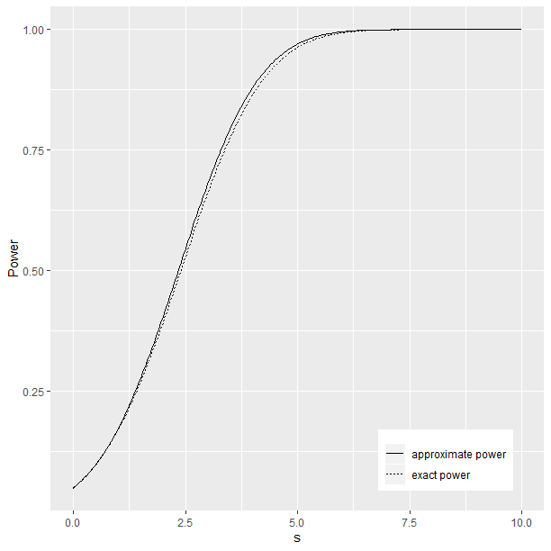
(b) Power comparison when $m=n=10$

Figure 1: Comparison of exact and approximate power.

We now discuss the power behavior of $T_{n,m}$ based on the Euclidean energy distance. In Case S2, it can be seen that

$$\sigma_{X}^{2}=\lim_{p\to\infty}\frac{1}{\tau^{2}_{X}}\displaystyle\sum_{i,i^{\prime}=1}^{p}4\,\textrm{tr}\,\Sigma_{X}^{2}(i,i^{\prime}),$$ (29)

where $\Sigma_{X}^{2}(i,i^{\prime})$ is the covariance matrix between $X_{(i)}$ and $X_{(i^{\prime})}$, and similar expressions for $\sigma_{Y}^{2}$. In case S2 (i.e., when $K$ is the Euclidean distance), if we further assume $\mu_{X}=\mu_{Y}$, it can be verified that

$$\sigma^{2}\;=\;\displaystyle\lim_{p\to\infty}\,\frac{1}{\tau^{2}}\displaystyle\sum_{i,i^{\prime}=1}^{p}4\,\textrm{tr}\big{(}\Sigma_{X}(i,i^{\prime})\,\Sigma_{Y}(i,i^{\prime})\big{)}\,.$$ (30)

Hence in Case S2, under the assumptions that $\mu_{X}=\mu_{Y}$, $\textrm{tr}\,\Sigma_{X}=\textrm{tr}\,\Sigma_{Y}$ and $\textrm{tr}\,\Sigma_{X}^{2}=\textrm{tr}\,\Sigma_{Y}^{2}=\textrm{tr}\,\Sigma_{X}\Sigma_{Y}$, it can be easily seen from equations (21), (29) and (30) that

$$\tau_{X}^{2}=\tau_{Y}^{2}=\tau^{2},\quad\sigma_{X}^{2}=\sigma_{Y}^{2}=\sigma^{2},$$ (31)

which implies that $\Delta^{*}_{0}=0$ in Proposition 4.2. Consider the following class of alternative distributions

$$H_{A}=\{(P_{X},P_{Y}):P_{X}\neq P_{Y},~{}\mu_{X}=\mu_{Y},~{}\textrm{tr}\,\Sigma_{X}=\textrm{tr}\,\Sigma_{Y},\,\textrm{tr}\,\Sigma_{X}^{2}=\textrm{tr}\,\Sigma_{Y}^{2}=\textrm{tr}\,\Sigma_{X}\Sigma_{Y}\}.$$

According to Theorem 4.2, the t-test $T_{n,m}$ based on Euclidean energy distance has trivial power against $H_{A}.$ In contrast, the t-test based on the proposed metrics has non-trivial power against $H_{A}$ as long as $\Delta^{*}_{0}>0.$

To summarize our contributions :

• We show that the Euclidean energy distance can only detect the equality of means and the traces of covariance matrices in the high-dimensional setup. To the best of our knowledge, such a limitation of the Euclidean energy distance has not been pointed out in the literature before.

• We propose a new class of homogeneity metrics which completely characterizes homogeneity of two distributions in the low-dimensional setup and has nontrivial power against a broader range of alternatives, or in other words, can detect a wider range of inhomogeneity of two distributions in the high-dimensional setup.

• Grouping allows us to detect homogeneity beyond univariate marginal distributions, as the difference between two univariate marginal distributions is automatically captured by the difference between the marginal distributions of the groups that contain these two univariate components.

• Consequently we construct a high-dimensional two-sample t-test whose computational cost is linear in $p$. Owing to the pivotal nature of the limiting distribution of the test statistic, no resampling-based inference is needed.

Remark 4.6.

Although the test based on our proposed statistic is asymptotically powerful against the alternative $H_{A}$ unlike the Euclidean energy distance, it can be verified that it has trivial power against the alternative $H_{A^{\prime}}=\{(X,Y):X_{(i)}\overset{d}{=}Y_{(i)},1\leq i\leq p\}$. Thus although it can detect differences between two high-dimensional distributions beyond the first two moments (as a significant improvement to the Euclidean energy distance), it cannot capture differences beyond the equality of the low-dimensional marginal distributions. We conjecture that there might be some intrinsic difficulties for distance and kernel-based metrics to completely characterize the discrepancy between two high-dimensional distributions.

5 Dependence metrics

In this section, we focus on dependence testing of two random vectors $X\in\mathbb{R}^{\tilde{p}}$ and $Y\in\mathbb{R}^{\tilde{q}}$. Suppose $X$ and $Y$ can be partitioned into $p$ and $q$ groups, viz. $X=\left(X_{(1)},X_{(2)},\dots,X_{(p)}\right)$ and $Y=\left(Y_{(1)},Y_{(2)},\dots,Y_{(q)}\right)$, where the components $X_{(i)}$ and $Y_{(j)}$ are $d_{i}$ and $g_{j}$ dimensional, respectively, for $1\leq i\leq p,1\leq j\leq q$. Here $p,q$ might be fixed or growing. We assume that $X_{(i)}$ and $Y_{(j)}$’s are finite (low) dimensional vectors, i.e., $\{d_{i}\}_{i=1}^{p}$ and $\{g_{j}\}_{j=1}^{q}$ are bounded sequences. Clearly, $\tilde{p}=\sum_{i=1}^{p}d_{i}=O(p)$ and $\tilde{q}=\sum_{j=1}^{q}g_{j}=O(q)$. We define a class of dependence metrics $\mathcal{D}$ between $X$ and $Y$ as the positive square root of

$$\mathcal{D}^{2}(X,Y)\;:=\;\mathbb{E}\,K_{\bf{d}}(X,X^{\prime})\,K_{\bf{g}}(Y,Y^{\prime})\,+\,\mathbb{E}\,K_{\bf{d}}(X,X^{\prime})\,\mathbb{E}\,K_{\bf{g}}(Y,Y^{\prime})\,-\,2\,\mathbb{E}\,K_{\bf{d}}(X,X^{\prime})\,K_{\bf{g}}(Y,Y^{\prime\prime})\,,$$ (32)

where ${\bf{d}}=(d_{1},\dots,d_{p})$ and ${\bf{g}}=(g_{1},\dots,g_{q})$. We drop the subscripts ${\bf{d}},{\bf{g}}$ of $K$ for notational convenience.

To ensure the existence of $\mathcal{D}$, we make the following assumption.

Assumption 5.1.

Assume that $\sup_{1\leq i\leq p}\mathbb{E}\rho_{i}^{1/2}(X_{(i)},0_{d_{i}})<\infty$ and $\sup_{1\leq i\leq q}\mathbb{E}\rho_{i}^{1/2}(Y_{(i)},0_{g_{i}})<\infty$.

In Section .2 of the supplement we demonstrate that in the low-dimensional setting, $\mathcal{D}(X,Y)$ completely characterizes independence between $X$ and $Y$. For an observed random sample $(X_{k},Y_{k})^{n}_{k=1}$ from the joint distribution of $X$ and $Y$, define $D^{X}:=(d^{X}_{kl})\in\mathbb{R}^{n\times n}$ with $d^{X}_{kl}:=K(X_{k},X_{l})$ and $k,l\in\{1,\dots,n\}$. Define $d^{Y}_{kl}$ and $D^{Y}$ in a similar way. With some abuse of notation, we consider the U-statistic type estimator $\widetilde{\mathcal{D}^{2}_{n}}(X,Y)$ of $\mathcal{D}^{2}$ as defined in (14) with $d_{\mathcal{X}}$ and $d_{\mathcal{Y}}$ being $K_{\mathbf{d}}$ and $K_{\mathbf{g}}$ respectively. In Section .2 of the supplement, we illustrate that $\widetilde{\mathcal{D}^{2}_{n}}(X,Y)$ essentially inherits all the nice properties of the U-statistic type estimator of generalized dCov and HSIC.

In the subsequent discussion we study the asymptotic behavior of $\mathcal{D}$ in the high-dimensional framework, i.e., when $p$ and $q$ grow to $\infty$ with fixed $n$ (discussed in Subsection 5.1) and when $n$ grows to $\infty$ as well (discussed in Subsection .2 in the supplement).

5.1 High dimension low sample size (HDLSS)

In this subsection, our goal is to explore the behavior of $\mathcal{D}^{2}(X,Y)$ and its unbiased U-statistic type estimator in the HDLSS setting where $p$ and $q$ grow to $\infty$ while the sample size $n$ is held fixed. Denote $\tau^{2}_{XY}=\tau^{2}_{X}\tau^{2}_{Y}=\mathbb{E}\,K^{2}(X,X^{\prime})\,\mathbb{E}\,K^{2}(Y,Y^{\prime}).$ We impose the following conditions.

Assumption 5.2.

$\mathbb{E}\,[L^{2}(X,X^{\prime})]=O(a_{p}^{\prime 2})$ and $\mathbb{E}\,[L^{2}(Y,Y^{\prime})]=O(b_{q}^{\prime 2})$, where $a_{p}^{\prime}$ and $b_{q}^{\prime}$ are positive real sequences satisfying $a_{p}^{\prime}=o(1)$, $b_{q}^{\prime}=o(1)$, $\tau_{XY}\,a_{p}^{\prime 2}b_{q}^{\prime}=o(1)$ and $\tau_{XY}\,a_{p}^{\prime}b_{q}^{\prime 2}=o(1)$. Further assume that $\mathbb{E}\,[R^{2}(X,X^{\prime})]=O(a_{p}^{\prime 4})$ and $\mathbb{E}\,[R^{2}(Y,Y^{\prime})]=O(b_{q}^{\prime 4})$.

Remark 5.1.

We refer the reader to Remark 4.1 in Section 4 for illustrations about some sufficient conditions under which we have ${\mbox{var}}\left(L(X,X^{\prime})\right)\,=\,\mathbb{E}\,L^{2}(X,X^{\prime})\,=\,O(\frac{1}{p})$, and similarly for $L(Y,Y^{\prime})$. Remark .1 in the supplement illustrates certain sufficient conditions under which $\mathbb{E}\,[R^{2}(X,X^{\prime})]=O(\frac{1}{p^{2}})$, and similarly for $R(Y,Y^{\prime})$.

Theorem 5.1.

Under Assumptions 4.2 and 5.2, we have

$$\mathcal{D}^{2}(X,Y)=\frac{1}{4\tau_{XY}}\displaystyle\sum_{i=1}^{p}\sum_{j=1}^{q}D^{2}_{\rho_{i},\rho_{j}}(X_{(i)},Y_{(j)})\,+\,\mathcal{R}\;,$$ (33)

where $\mathcal{R}$ is the remainder term such that $\mathcal{R}=O(\tau_{XY}\,a_{p}^{\prime 2}b_{q}^{\prime}+\tau_{XY}\,a_{p}^{\prime}b_{q}^{\prime 2})=o(1)$.

Theorem 5.1 shows that when dimensions grow high, the population $\mathcal{D}^{2}(X,Y)$ behaves as an aggregation of group-wise generalized dCov and thus essentially captures group-wise non-linear dependencies between $X$ and $Y$.

Remark 5.2.

Consider a special case where $d_{i}=1$ and $g_{j}=1$, and $\rho_{i}$ and $\rho_{j}$ are Euclidean distances for all $1\leq i\leq p$ and $1\leq j\leq q$. Then Theorem 5.1 essentially boils down to

$$\mathcal{D}^{2}(X,Y)=\frac{1}{4\tau_{XY}}\displaystyle\sum_{i=1}^{p}\sum_{j=1}^{q}dCov^{2}(X_{i},Y_{j})\,+\,\mathcal{R}\;,$$ (34)

where $\mathcal{R}=o(1)$. This shows that in a special case (when we have unit group sizes), $\mathcal{D}^{2}(X,Y)$ essentially behaves as an aggregation of cross-component dCov between $X$ and $Y$. If $K_{\textbf{d}}$ and $K_{\textbf{g}}$ are Euclidean distances, or in other words if each $\rho_{i}$ and $\rho_{j}$ are squared Euclidean distances, then using equation (10) it is straightforward to verify that $D^{2}_{\rho_{i},\rho_{j}}(X_{i},Y_{j})=4\,cov^{2}(X_{i},Y_{j})$ for all $1\leq i\leq p$ and $1\leq j\leq q$. Consequently we have

$$\mathcal{D}^{2}(X,Y)=dCov^{2}(X,Y)=\frac{1}{\tau_{XY}}\displaystyle\sum_{i=1}^{p}\sum_{j=1}^{q}cov^{2}(X_{i},Y_{j})\,+\,\mathcal{R}_{1}\;,$$ (35)

where $\mathcal{R}_{1}=o(1)$, which essentially presents a population version of Theorem 2.1.1 in Zhu et al. (2019) as a special case of Theorem 5.1.

Remark 5.3.

To illustrate that the leading term in equation (33) indeed gives a close approximation of the population $\mathcal{D}^{2}(X,Y)$, we consider the special case when $K_{\textbf{d}}$ and $K_{\textbf{g}}$ are Euclidean distances and $p=q$. Suppose $X\sim N_{p}(0,I_{p})$ and $Y=X+N$ where $N\sim N_{p}(0,I_{p})$ with $N\mathrel{\text{\scalebox{1.07}{$\perp\mkern-10.0mu\perp$}}}X$. Clearly we have $\tau_{X}^{2}=2p$, $\tau_{Y}^{2}=4p$, $D^{2}_{\rho_{i},\rho_{j}}(X_{i},Y_{j})=4\,cov^{2}(X_{i},Y_{j})=4$  for all  $1\leq i=j\leq p$ and $D^{2}_{\rho_{i},\rho_{j}}(X_{i},Y_{j})=0$ for all  $1\leq i\neq j\leq p$. From Remark 5.2, it is clear that in this case we essentially have $\mathcal{D}^{2}(X,Y)=dCov^{2}(X,Y)$. We simulate a large sample of size $n=5000$ from the distribution of $(X,Y)$ for $p=20,40,60,80$ and $100$. The large sample size is to ensure that the U-statistic type estimator of $\mathcal{D}^{2}(X,Y)$ (given in (14)) gives a very close approximation of the population $\mathcal{D}^{2}(X,Y)$. We list the ratio between $\mathcal{D}^{2}(X,Y)$ and the leading term in (33) for the different values of $p$, which turn out to be very close to $1$, demonstrating that the leading term in (33) indeed approximates $\mathcal{D}^{2}(X,Y)$ reasonably well.

Table 2: Ratio of $\mathcal{D}^{2}(X,Y)$ and the leading term in (33) for different values of $p$.

$p=20$	$p=40$	$p=60$	$p=80$	$p=100$
0.980	0.993	0.994	0.989	0.997

The following theorem explores the behavior of the population $\mathcal{D}^{2}(X,Y)$ when $p$ is fixed and $q$ grows to infinity, while the sample size is held fixed. As far as we know, this asymptotic regime has not been previously considered in the literature. In this case, the Euclidean distance covariance behaves as an aggregation of martingale difference divergences proposed in Shao and Zhang (2014) which measures conditional mean dependence. Figure 2 below summarizes the curse of dimensionality for the Euclidean distance covariance under different asymptotic regimes.

Theorem 5.2.

Under Assumption 4.2 and the assumption that  $\mathbb{E}\,[R^{2}(Y,Y^{\prime})]=O(b_{q}^{\prime 4})$ with $\tau_{Y}\,b_{q}^{\prime 2}=o(1)$, as $q\to\infty$ with $p$ and $n$ remaining fixed, we have

$$\mathcal{D}^{2}(X,Y)\; =\;\frac{1}{2\tau_{Y}}\displaystyle\sum_{j=1}^{q}D^{2}_{K_{\textbf{d}}\,,\rho_{j}}(X,Y_{(j)})\,+\,\mathcal{R},$$

where $\mathcal{R}$ is the remainder term such that $\mathcal{R}=O(\tau_{Y}\,b_{q}^{\prime 2})=o(1)$.

Remark 5.4.

In particular, when both $K_{\textbf{d}}$ and $K_{\textbf{g}}$ are Euclidean distances, we have

$$\mathcal{D}^{2}(X,Y)\; =\;dCov^{2}(X,Y)\;=\;\frac{1}{\tau_{Y}}\displaystyle\sum_{j=1}^{\tilde{q}}MDD^{2}(Y_{j}|X)\,+\,\mathcal{R},$$

where $MDD^{2}(Y_{j}|X)=-\mathbb{E}[(Y_{j}-\mathbb{E}Y_{j})(Y_{j}^{\prime}-\mathbb{E}Y_{j})\|X-X^{\prime}\|]$ is the martingale difference divergence which completely characterizes the conditional mean dependence of $Y_{j}$ given $X$ in the sense that $E[Y_{j}|X]=E[Y_{j}]$ almost surely if and only if $MDD^{2}(Y_{j}|X)=0.$

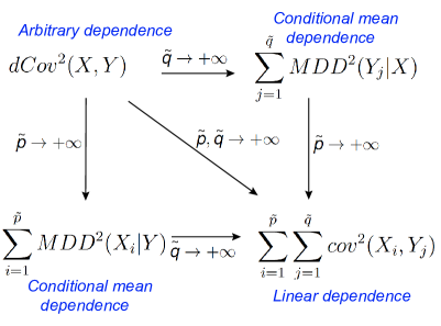
Figure 2: Curse of dimensionality for the Euclidean distance covariance under different asymptotic regimes

Next we study the asymptotic behavior of the sample version $\widetilde{\mathcal{D}^{2}_{n}}(X,Y)$.

Assumption 5.3.

Assume that $L(X,X^{\prime})=O_{p}(a_{p})$ and $L(Y,Y^{\prime})=O_{p}(b_{q})$, where $a_{p}$ and $b_{q}$ are positive real sequences satisfying $a_{p}=o(1)$, $b_{q}=o(1)$, $\tau_{XY}\,a_{p}^{2}b_{q}=o(1)$ and $\tau_{XY}\,a_{p}b_{q}^{2}=o(1)$.

Remark 5.5.

We refer the reader to Remark 4.1 in Section 4 for illustrations about Assumption 5.3.

Theorem 5.3.

Under Assumptions 4.2 and 5.3, it can be shown that

$$\widetilde{\mathcal{D}^{2}_{n}}(X,Y)=\frac{1}{4\tau_{XY}}\displaystyle\sum_{i=1}^{p}\sum_{j=1}^{q}\widetilde{D^{2}_{n}}_{\,;\,\rho_{i},\rho_{j}}(X_{(i)},Y_{(j)})\,+\,\mathcal{R}_{n}\;,$$ (36)

where $X_{(i)},Y_{(j)}$ are the $i^{th}$ and $j^{th}$ groups of $X$ and $Y$, respectively, $1\leq i\leq p$, $1\leq j\leq q$ , and $\mathcal{R}_{n}$ is the remainder term. Moreover $\mathcal{R}_{n}=O_{p}(\tau_{XY}\,a_{p}^{2}b_{q}+\tau_{XY}\,a_{p}b_{q}^{2})=o_{p}(1)$, i.e., $\mathcal{R}_{n}$ is of smaller order compared to the leading term and hence is asymptotically negligible.

The above theorem generalizes Theorem 2.1.1 in Zhu et al. (2019) by showing that the leading term of $\widetilde{\mathcal{D}^{2}_{n}}(X,Y)$ is the sum of all the group-wise (unbiased) squared sample generalized dCov scaled by $\tau_{XY}\,$. In other words, in the HDLSS setting, $\widetilde{\mathcal{D}^{2}_{n}}(X,Y)$ is asymptotically equivalent to the aggregation of group-wise squared sample generalized dCov. Thus $\widetilde{\mathcal{D}^{2}_{n}}(X,Y)$ can quantify group-wise non-linear dependencies between $X$ and $Y$, going beyond the scope of the usual Euclidean dCov.

Remark 5.6.

Consider a special case where $d_{i}=1$ and $g_{j}=1$, and $\rho_{i}$ and $\rho_{j}$ are Euclidean distances for all $1\leq i\leq p$ and $1\leq j\leq q$. Then Theorem 5.3 essentially states that

$$\widetilde{\mathcal{D}^{2}_{n}}(X,Y)=\frac{1}{4\tau_{XY}}\displaystyle\sum_{i=1}^{p}\sum_{j=1}^{q}dCov^{2}_{n}(X_{i},Y_{j})\,+\,\mathcal{R}_{n}\;,$$ (37)

where $\mathcal{R}_{n}=o_{p}(1)$. This demonstrates that in a special case (when we have unit group sizes), $\widetilde{\mathcal{D}^{2}_{n}}(X,Y)$ is asymptotically equivalent to the marginal aggregation of cross-component distance covariances proposed by Zhu et al. (2019) as dimensions grow high. If $K_{\textbf{d}}$ and $K_{\textbf{g}}$ are Euclidean distances, then Theorem 5.3 essentially boils down to Theorem 2.1.1 in Zhu et al. (2019) as a special case.

Remark 5.7.

To illustrate the approximation of $\widetilde{\mathcal{D}^{2}_{n}}(X,Y)$ by the aggregation of group-wise squared sample generalized dCov given by Theorem 5.3, we simulated the datasets in Examples 6.4.1, 6.4.2, 6.5.1 and 6.5.2  $100$ times each with $n=50$ and $p=q=50$. For each of the datasets, the difference between $\widetilde{\mathcal{D}^{2}_{n}}(X,Y)$ and the leading term in the RHS of equation (36) is smaller than $0.01$ $100\%$ of the times, which illustrates that the approximation works reasonably well.

The following theorem illustrates the asymptotic behavior of $\widetilde{\mathcal{D}^{2}_{n}}(X,Y)$ when $p$ is fixed and $q$ grows to infinity while the sample size is held fixed. Under this setup, if both $K_{\textbf{d}}$ and $K_{\textbf{g}}$ are Euclidean distances, the leading term of $\widetilde{\mathcal{D}^{2}_{n}}(X,Y)$ is the sum of the group-wise unbiased U-statistic type estimators of $MDD^{2}(Y_{j}|X)$ for $1\leq j\leq q$, scaled by $\tau_{Y}\,$. In other words, the sample Euclidean distance covariance behaves as an aggregation of sample martingale difference divergences.

Theorem 5.4.

Under Assumption 4.2 and the assumption that  $L(Y,Y^{\prime})=O_{p}(b_{q})$ with $b_{q}=o(1)$ and  $\tau_{Y}\,b_{q}^{2}=o(1)$, as  $q\to\infty$ with $p$ and $n$ remaining fixed, we have

$$\widetilde{\mathcal{D}^{2}_{n}}(X,Y)\; =\;\frac{1}{2\tau_{Y}}\displaystyle\sum_{j=1}^{q}\widetilde{\mathcal{D}^{2}_{n}}_{\,;\,K_{\textbf{d}}\,,\rho_{j}}(X,Y_{(j)})\,+\,\mathcal{R}_{n},$$

where $\mathcal{R}_{n}$ is the remainder term such that $\mathcal{R}_{n}=O_{p}(\tau_{Y}\,b_{q}^{2})=o_{p}(1)$.

Remark 5.8.

In particular, when both $K_{\textbf{d}}$ and $K_{\textbf{g}}$ are Euclidean distances, we have

$$\widetilde{\mathcal{D}^{2}_{n}}(X,Y)\; =\;dCov^{2}_{n}(X,Y)\;=\;\frac{1}{\tau_{Y}}\displaystyle\sum_{j=1}^{\tilde{q}}MDD^{2}_{n}(Y_{j}|X)\,+\,\mathcal{R}_{n},$$

where $MDD^{2}_{n}(Y_{j}|X)$ is the unbiased U-statistic type estimator of $MDD^{2}(Y_{j}|X)$ defined as in (14) with $d_{\mathcal{X}}(x,x^{\prime})=\|x-x^{\prime}\|$ for $x,x^{\prime}\in\mathbb{R}^{\tilde{p}}$ and $d_{\mathcal{Y}}(y,y^{\prime})=|y-y^{\prime}|^{2}/2$ for $y,y^{\prime}\in\mathbb{R}$, respectively.

Now denote $X_{k}=(X_{k(1)},\dots,X_{k(p)})$ and $Y_{k}=(Y_{k(1)},\dots,Y_{k(q)})$ for $1\leq k\leq n$. Define the leading term of $\widetilde{\mathcal{D}^{2}_{n}}(X,Y)$ in equation (36) as

$$L:=\,\frac{1}{4\tau_{XY}\,}\sum_{i=1}^{p}\sum_{j=1}^{q}\widetilde{D^{2}_{n}}_{\,;\,\rho_{i},\rho_{j}}(X_{(i)},Y_{(j)})\,.$$

It can be verified that

$$L\,=\,\frac{1}{4\tau_{XY}\,}\sum_{i=1}^{p}\sum_{j=1}^{q}\left(\tilde{D}^{X}(i)\cdot\tilde{D}^{Y}(j)\right)\,,$$

where $\tilde{D}^{X}(i),\tilde{D}^{Y}(j)$ are the $\mathcal{U}$-centered versions of $D^{X}(i)=\left(d^{X}_{kl}(i)\right)_{k,l=1}^{n}$ and $D^{Y}(j)=\left(d^{Y}_{kl}(j)\right)_{k,l=1}^{n}$, respectively. As an advantage of using the double-centered distances, we have for all $1\leq i,i^{\prime}\leq p$, $1\leq j,j^{\prime}\leq q$ and $\{k,l\}\neq\{u,v\},$

$$\mathbb{E}\left[d^{X}_{kl}(i)\,d^{X}_{uv}(i^{\prime})\right]\;=\;\mathbb{E}\left[d^{Y}_{kl}(j)\,d^{Y}_{uv}(j^{\prime})\right]\;=\;\mathbb{E}\left[d^{X}_{kl}(i)\,d^{Y}_{uv}(j)\right]\;=\;0.$$ (38)

See for example the proof of Proposition 2.2.1 in Zhu et al. (2019) for a detailed explanation.

Assumption 5.4.

For fixed $n$, as $p,q\to\infty$,

$$\begin{pmatrix}\frac{1}{2\,\tau_{X}}\displaystyle\sum_{i=1}^{p}d^{X}_{kl}(i)\\ \frac{1}{2\,\tau_{Y}}\displaystyle\sum_{j=1}^{q}d^{Y}_{uv}(j)\end{pmatrix}_{k<l,\,u<v}\overset{d}{\longrightarrow}\;\;\begin{pmatrix}d_{kl}^{1}\\ \\ d_{uv}^{2}\end{pmatrix}_{k<l,\,u<v}\,,$$

where $\{d_{kl}^{1},\,d_{uv}^{2}\}_{k<l,\,u<v}$ are jointly Gaussian. Further we assume that

$$var(d_{kl}^{1}):=\sigma_{X}^{2}=\lim_{p\to\infty}\,\frac{1}{4\tau_{X}^{2}}\displaystyle\sum_{i,i^{\prime}=1}^{p}D^{2}_{\rho_{i},\rho_{i^{\prime}}}\left(X_{(i)},X_{(i^{\prime})}\right),$$

$$var(d_{kl}^{2}):=\sigma_{Y}^{2}=\lim_{q\to\infty}\,\frac{1}{4\tau_{Y}^{2}}\displaystyle\sum_{j,j^{\prime}=1}^{q}D^{2}_{\rho_{j},\rho_{j^{\prime}}}\left(Y_{(j)},Y_{(j^{\prime})}\right),$$

$${\mbox{cov}}\,(d_{kl}^{1},d_{kl}^{2}):=\sigma_{XY}^{2}=\lim_{p,q\to\infty}\,\frac{1}{4\tau_{XY}}\displaystyle\sum_{i=1}^{p}\sum_{j=1}^{q}D^{2}_{\rho_{i},\rho_{j}}\left(X_{(i)},Y_{(j)}\right).$$

In view of (38), we have ${\mbox{cov}}\,(d_{kl}^{1},d_{uv}^{1})={\mbox{cov}}\,(d_{kl}^{2},d_{uv}^{2})={\mbox{cov}}\,(d_{kl}^{1},d_{uv}^{2})=0$ for $\{k,l\}\neq\{u,v\}$. Theorem 5.3 states that for growing $p$ and $q$ and fixed $n$, $\widetilde{\mathcal{D}^{2}_{n}}(X,Y)$ and $L$ are asymptotically equivalent. By studying the leading term, we obtain the limiting distribution of $\widetilde{\mathcal{D}^{2}_{n}}(X,Y)$ as follows.

Theorem 5.5.

Under Assumptions 4.2, 5.3 and 5.4, for fixed $n$ and $p,q\to\infty$,

$$\widetilde{\mathcal{D}^{2}_{n}}(X,Y)\;\overset{d}{\longrightarrow}\;\frac{1}{\nu}d^{1\top}Md^{2}\,,$$

$$\widetilde{\mathcal{D}^{2}_{n}}(X,X)\;\overset{d}{\longrightarrow}\;\frac{1}{\nu}d^{1\top}Md^{1}\;\overset{d}{=}\;\frac{\sigma_{X}^{2}}{\nu}\chi^{2}_{\nu}\,,$$

$$\widetilde{\mathcal{D}^{2}_{n}}(Y,Y)\;\overset{d}{\longrightarrow}\;\frac{1}{\nu}d^{2\top}Md^{2}\;\overset{d}{=}\;\frac{\sigma_{Y}^{2}}{\nu}\chi^{2}_{\nu}\,,$$

where $M$ is a projection matrix of rank  $\nu=\frac{n(n-3)}{2}$, and

$$\begin{pmatrix}d^{1}\\ d^{2}\end{pmatrix}\;\sim\;N\left(0\,,\begin{pmatrix}\sigma_{X}^{2}\,I_{\frac{n(n-1)}{2}}\;\;\sigma_{XY}^{2}\,I_{\frac{n(n-1)}{2}}\\ \\ \sigma_{XY}^{2}\,I_{\frac{n(n-1)}{2}}\;\;\sigma_{Y}^{2}\,I_{\frac{n(n-1)}{2}}\end{pmatrix}\right)\,.$$

To perform independence testing, in the spirit of Székely and Rizzo (2014), we define the studentized test statistic

$$\mathcal{T}_{n}\;:=\;\sqrt{\nu-1}\,\frac{\widetilde{\mathcal{DC}^{2}_{n}}(X,Y)}{\sqrt{1-\left(\widetilde{\mathcal{DC}^{2}_{n}}(X,Y)\right)^{2}}}\;,$$ (39)

where

$$\widetilde{\mathcal{DC}^{2}_{n}}(X,Y)\;=\;\frac{\widetilde{\mathcal{D}^{2}_{n}}(X,Y)}{\sqrt{\widetilde{\mathcal{D}^{2}_{n}}(X,X)\,\widetilde{\mathcal{D}^{2}_{n}}(Y,Y)}}\,.$$

Define $\psi=\sigma_{XY}^{2}/\sqrt{\sigma_{X}^{2}\sigma_{Y}^{2}}$. The following theorem states the asymptotic distributions of the test statistic $\mathcal{T}_{n}$ under the null hypothesis $\tilde{H}_{0}:X\mathrel{\text{\scalebox{1.07}{$\perp\mkern-10.0mu\perp$}}}Y$ and the alternative hypothesis $\tilde{H}_{A}:X\centernot{\mathrel{\text{\scalebox{1.07}{$\perp\mkern-10.0mu\perp$}}}}Y$.

Theorem 5.6.

Under Assumptions 4.2, 5.3 and 5.4, for fixed $n$ and $p,q\to\infty$,

$$P_{\tilde{H}_{0}}\left(\mathcal{T}_{n}\leq t\right)\;\longrightarrow\;P\left(t_{\nu-1}\leq t\right),$$

$$P_{\tilde{H}_{A}}\left(\mathcal{T}_{n}\leq t\right)\;\longrightarrow\;\mathbb{E}\left[P\left(t_{\nu-1,W}\leq t|W\right)\right],$$

where $t$ is any fixed real number and $W\sim\sqrt{\frac{\psi^{2}}{1-\psi^{2}}\,\chi^{2}_{\nu}}$.

For an explicit form of $\mathbb{E}\left[P\left(t_{\nu-1,W}\leq t|W\right)\right]$, we refer the reader to Lemma 3 in the appendix of Zhu et al. (2019). Now consider the local alternative hypothesis $\tilde{H}_{A}^{*}$: $X\centernot{\mathrel{\text{\scalebox{1.07}{$\perp\mkern-10.0mu\perp$}}}}Y$ with $\psi=\psi_{0}/\sqrt{\nu}$, where $\psi_{0}$ is a constant with respect to $n$. The following proposition gives an approximation of $\mathbb{E}\left[P\left(t_{\nu-1,W}\leq t|W\right)\right]$ under the local alternative hypothesis $\tilde{H}_{A}^{*}$ when $n$ is allowed to grow.

Proposition 5.1.

Under $\tilde{H}_{A}^{*}$, as $n\to\infty$ and  $t=O(1)$,

$$\mathbb{E}\left[P\left(t_{\nu-1,W}\leq t|W\right)\right]\;=\;P\left(t_{\nu-1,\,\psi_{0}}\leq t\right)\;+\;O\Big{(}\frac{1}{\nu}\Big{)}\,.$$

The following summarizes our key findings in this section.

• Advantages of our proposed metrics over the Euclidean dCov and HSIC :

  1. Our proposed dependence metrics completely characterize independence between $X$ and $Y$ in the low-dimensional setup, and can detect group-wise non-linear dependencies between $X$ and $Y$ in the high-dimensional setup as opposed to merely detecting component-wise linear dependencies by the Euclidean dCov and HSIC (in light of Theorem 2.1.1 in Zhu et al. (2019)).

  2. We also showed that with $p$ remaining fixed and $q$ growing high, the Euclidean dCov can only quantify conditional mean independence of the components of $Y$ given $X$ (which is weaker than independence). To the best of our knowledge, this has not been pointed out in the literature before.

• Advantages over the marginal aggregation approach by Zhu et al. (2019) :

  1. In the low-dimensional setup, our proposed dependence metrics can completely characterize independence between $X$ and $Y$, whereas the metric proposed by Zhu et al. (2019) can only capture pairwise dependencies between the components of $X$ and $Y$.

  2. We provide a neater way of generalizing dCov and HSIC between $X$ and $Y$ which is shown to be asymptotically equivalent to the marginal aggregation of cross-component distance covariances proposed by Zhu et al. (2019) as dimensions grow high. Also grouping or partitioning the two high-dimensional random vectors (which again may be problem specific) allows us to detect a wider range of alternatives compared to only detecting component-wise non-linear dependencies, as independence of two univariate marginals is implied from independence of two higher dimensional marginals containing the two univariate marginals.

  3. The computational complexity of the (unbiased) squared sample $\mathcal{D}(X,Y)$ is $O(n^{2}(p+q))$. Thus the computational cost of our proposed two-sample t-test only grows linearly with the dimension and therefore is scalable to very high-dimensional data. Although a naive aggregation of marginal distance covariances has a computational complexity of $O(n^{2}pq)$, the approach of Zhu et al. (2019) essentially corresponds to the use of an additive kernel and the computational cost of their proposed estimator can also be made linear in the dimensions if properly implemented.

Table 3: Summary of the behaviors of the proposed homogeneity/dependence metrics for different choices of $\rho_{i}(x,x^{\prime})$ in high dimension.

Choice of $\rho_{i}(x,x^{\prime})$	Asymptotic behavior of the proposed homogeneity metric	Asymptotic behavior of the proposed dependence metric
the semi-metric $\|x-x^{\prime}\|^{2}$	Behaves as a sum of squared Euclidean distances	Behaves as a sum of squared Pearson correlations
metric of strong negative type on $\mathbb{R}^{d_{i}}$	Behaves as a sum of groupwise energy distances with the metric $\rho_{i}$	Behaves as a sum of groupwise dCov with the metric $\rho_{i}$
$k_{i}(x,x)+k_{i}(x^{\prime},x^{\prime})-2k_{i}(x,x^{\prime})$, where $k_{i}$ is a characteristic kernel on $\mathbb{R}^{d_{i}}\times\mathbb{R}^{d_{i}}$	Behaves as a sum of groupwise MMD with the kernel $k_{i}$	Behaves as a sum of groupwise HSIC with the kernel $k_{i}$

6 Numerical studies

6.1 Testing for homogeneity of distributions

We investigate the empirical size and power of the tests for homogeneity of two high dimensional distributions. For comparison, we consider the t-tests based on the following metrics:

1. $\mathcal{E}$ with $\rho_{i}$ as the Euclidean distance for $1\leq i\leq p$;

2. $\mathcal{E}$ with $\rho_{i}$ as the distance induced by the Laplace kernel for $1\leq i\leq p$;

3. $\mathcal{E}$ with $\rho_{i}$ as the distance induced by the Gaussian kernel for $1\leq i\leq p$;

4. the usual Euclidean energy distance;

5. MMD with the Laplace kernel;

6. MMD with the Gaussian kernel.

We set $d_{i}=1$ in Examples 6.1 and 6.2, and $d_{i}=2$ in Example 6.3 for $1\leq i\leq p$.

Example 6.1.

Consider $X_{k}=(X_{k1},\dots,X_{kp})$  and  $Y_{l}=(Y_{l1},\dots,Y_{lp})$ with $k=1,\dots,n$ and $l=1,\dots,m$. We generate i.i.d. samples from the following models:

1. $X_{k}\sim N(0,I_{p})$  and  $Y_{l}\sim N(0,I_{p})$.

2. $X_{k}\sim N(0,\Sigma)$  and  $Y_{l}\sim N(0,\Sigma)$, where $\Sigma=(\sigma_{ij})_{i,j=1}^{p}$ with $\sigma_{ii}=1$ for  $i=1,\dots,p$, $\sigma_{ij}=0.25$ if $1\leq|i-j|\leq 2$ and $\sigma_{ij}=0$ otherwise.

3. $X_{k}\sim N(0,\Sigma)$  and  $Y_{l}\sim N(0,\Sigma)$, where $\Sigma=(\sigma_{ij})_{i,j=1}^{p}$ with $\sigma_{ij}=0.7^{|i-j|}$.

Example 6.2.

Consider $X_{k}=(X_{k1},\dots,X_{kp})$  and  $Y_{l}=(Y_{l1},\dots,Y_{lp})$ with $k=1,\dots,n$ and $l=1,\dots,m$. We generate i.i.d. samples from the following models:

1. $X_{k}\sim N(\mu,I_{p})$ with $\mu=(1,\dots,1)\in\mathbb{R}^{p}$  and  $Y_{li}\overset{ind}{\sim}$ Poisson $(1)$ for $i=1,\dots,p$.

2. $X_{k}\sim N(\mu,I_{p})$ with $\mu=(1,\dots,1)\in\mathbb{R}^{p}$  and  $Y_{li}\overset{ind}{\sim}$ Exponential $(1)$ for $i=1,\dots,p$.

3. $X_{k}\sim N(0,I_{p})$  and  $Y_{l}=(Y_{l1},\dots,Y_{l\lfloor\beta p\rfloor},Y_{l(\lfloor\beta p\rfloor+1)},\dots,Y_{lp})$, where $Y_{l1},\dots,Y_{l\lfloor\beta p\rfloor}\overset{i.i.d.}{\sim}$ Rademacher $(0.5)$  and  $Y_{l(\lfloor\beta p\rfloor+1)},\dots,Y_{lp}\overset{i.i.d.}{\sim}N(0,1)$.

4. $X_{k}\sim N(0,I_{p})$  and  $Y_{l}=(Y_{l1},\dots,Y_{l\lfloor\beta p\rfloor},Y_{l(\lfloor\beta p\rfloor+1)},\dots,Y_{lp})$, where $Y_{l1},\dots,Y_{l\lfloor\beta p\rfloor}\overset{i.i.d.}{\sim}$ Uniform $(-\sqrt{3},\sqrt{3})$  and  $Y_{l(\lfloor\beta p\rfloor+1)},\dots,Y_{lp}\overset{i.i.d.}{\sim}N(0,1)$.

5. $X_{k}=R^{1/2}Z_{1k}$ and $Y_{l}=R^{1/2}Z_{2l}$, where $R=(r_{ij})_{i,j=1}^{p}$ with $r_{ii}=1$ for  $i=1,\dots,p$, $r_{ij}=0.25$ if $1\leq|i-j|\leq 2$ and $r_{ij}=0$ otherwise, $Z_{1k}\sim N(0,I_{p})$ and $Z_{2l}=\underbrace{(Z_{2l1},\dots,Z_{2lp})}_{\overset{i.i.d.}{\sim}Exponential(1)}-\,1.$

Example 6.3.

Consider $X_{k}=(X_{k(1)},\dots,X_{k(p)})$  and  $Y_{l}=(Y_{l(1)},\dots,Y_{l(p)})$ with $k=1,\dots,n$ and $l=1,\dots,m$  and  $d_{i}=2$ for $1\leq i\leq p$. We generate i.i.d. samples from the following models:

1. $X_{k(i)}\sim N(\mu,\Sigma_{1})$  and  $Y_{l(i)}\sim N(\mu,\Sigma_{2})$ with $X_{k(i)}\mathrel{\text{\scalebox{1.07}{$\perp\mkern-10.0mu\perp$}}}X_{k(j)}$ and $Y_{l(i)}\mathrel{\text{\scalebox{1.07}{$\perp\mkern-10.0mu\perp$}}}Y_{l(j)}$ for $1\leq i\neq j\leq p$, where $\mu=(1,1)^{\top}$, $\Sigma_{1}=\begin{pmatrix}1&0.9\\ 0.9&1\end{pmatrix}$ and  $\Sigma_{2}=\begin{pmatrix}1&0.1\\ 0.1&1\end{pmatrix}$.

2. $X_{k(i)}\sim N(\mu,\Sigma)$ with $X_{k(i)}\mathrel{\text{\scalebox{1.07}{$\perp\mkern-10.0mu\perp$}}}X_{k(j)}$ for $1\leq i\neq j\leq p$, where $\mu=(1,1)^{\top}$, $\Sigma=\begin{pmatrix}1&0.7\\ 0.7&1\end{pmatrix}$. The components of  $Y_{l}$ are i.i.d. Exponential $(1)$.

Note that for Examples 6.1 and 6.2, the metric defined in equation (15) essentially boils down to the special case in equation (17). We try small sample sizes $n=m=50$, dimensions $p=q=50,100$ and $200$, and $\beta=1/2$. Table 4 reports the proportion of rejections out of $1000$ simulation runs for the different tests. For the tests V and VI, we chose the bandwidth parameter heuristically as the median distance between the aggregated sample observations. For tests II and III, the bandwidth parameters are chosen using the median heuristic separately for each group.

In Example 6.1, the data generating scheme suggests that the variables $X$ and $Y$ are identically distributed. The results in Table 4 show that the tests based on both the proposed homogeneity metrics and the usual Euclidean energy distance and MMD perform more or less equally good, and the rejection probabilities are quite close to the $10\%$ or $5\%$ nominal level. In Example 6.2, clearly $X$ and $Y$ have different distributions but $\mu_{X}=\mu_{Y}$ and $\Sigma_{X}=\Sigma_{Y}$. The results in Table 4 indicate that the tests based on the proposed homogeneity metrics are able to detect the differences between the two high-dimensional distributions beyond the first two moments unlike the tests based on the usual Euclidean energy distance and MMD, and thereby outperform the latter in terms of empirical power. In Example 6.3, clearly $\mu_{X}=\mu_{Y}$ and $\textrm{tr}\,\Sigma_{X}=\textrm{tr}\,\Sigma_{Y}$ and the results show that the tests based on the proposed homogeneity metrics are able to detect the in-homogeneity of the low-dimensional marginal distributions unlike the tests based on the usual Euclidean energy distance and MMD.

Table 4: Empirical size and power for the different tests of homogeneity of distributions.

					I		II		III		IV		V		VI
		$n$	$m$	$p$	10%	5%	10%	5%	10%	5%	10%	5%	10%	5%	10%	5%
Ex 6.1	(1)	50	50	50	0.109	0.062	0.109	0.058	0.106	0.063	0.109	0.068	0.110	0.069	0.109	0.070
	(1)	50	50	100	0.124	0.073	0.119	0.053	0.121	0.063	0.116	0.067	0.114	0.068	0.117	0.068
	(1)	50	50	200	0.086	0.043	0.099	0.048	0.088	0.035	0.090	0.045	0.086	0.043	0.090	0.045
	(2)	50	50	50	0.114	0.069	0.108	0.054	0.118	0.068	0.116	0.077	0.115	0.073	0.116	0.078
	(2)	50	50	100	0.130	0.069	0.133	0.073	0.124	0.070	0.126	0.067	0.123	0.068	0.124	0.067
	(2)	50	50	200	0.099	0.048	0.103	0.041	0.092	0.047	0.097	0.040	0.095	0.039	0.097	0.040
	(3)	50	50	50	0.100	0.064	0.107	0.057	0.099	0.060	0.112	0.072	0.105	0.067	0.110	0.073
	(3)	50	50	100	0.103	0.062	0.113	0.061	0.113	0.063	0.097	0.060	0.100	0.057	0.098	0.059
	(3)	50	50	200	0.108	0.062	0.115	0.062	0.117	0.064	0.091	0.055	0.093	0.056	0.090	0.055
Ex 6.2	(1)	50	50	50	1	1	1	1	0.995	0.994	0.102	0.067	0.111	0.069	0.103	0.066
	(1)	50	50	100	1	1	1	1	1	1	0.120	0.066	0.120	0.071	0.119	0.066
	(1)	50	50	200	1	1	1	1	1	1	0.111	0.057	0.111	0.057	0.111	0.057
	(2)	50	50	50	1	1	1	1	1	1	0.126	0.085	0.154	0.105	0.119	0.073
	(2)	50	50	100	1	1	1	1	1	1	0.098	0.058	0.108	0.066	0.094	0.055
	(2)	50	50	200	1	1	1	1	1	1	0.111	0.055	0.114	0.056	0.108	0.054
	(3)	50	50	50	1	1	1	1	1	0.999	0.118	0.069	0.117	0.072	0.120	0.070
	(3)	50	50	100	1	1	1	1	1	1	0.102	0.067	0.106	0.065	0.103	0.067
	(3)	50	50	200	1	1	1	1	1	1	0.103	0.046	0.103	0.049	0.102	0.046
	(4)	50	50	50	0.452	0.328	0.863	0.771	0.552	0.421	0.114	0.061	0.111	0.061	0.114	0.061
	(4)	50	50	100	0.640	0.491	0.990	0.967	0.761	0.637	0.098	0.063	0.104	0.063	0.098	0.062
	(4)	50	50	200	0.840	0.733	1	0.999	0.933	0.876	0.105	0.042	0.108	0.042	0.105	0.043
	(5)	50	50	50	1	1	1	1	1	1	0.128	0.078	0.163	0.098	0.115	0.077
	(5)	50	50	100	1	1	1	1	1	1	0.098	0.053	0.115	0.063	0.091	0.051
	(5)	50	50	200	1	1	1	1	1	1	0.100	0.050	0.103	0.054	0.098	0.050
Ex 6.3	(1)	50	50	50	1	1	1	1	1	1	0.157	0.098	0.223	0.137	0.156	0.098
	(1)	50	50	100	1	1	1	1	1	1	0.158	0.089	0.188	0.124	0.157	0.090
	(1)	50	50	200	1	1	1	1	1	1	0.122	0.074	0.161	0.091	0.121	0.074
	(2)	50	50	50	1	1	1	1	1	1	0.140	0.078	0.190	0.118	0.137	0.075
	(2)	50	50	100	1	1	1	1	1	1	0.139	0.080	0.171	0.105	0.136	0.080
	(2)	50	50	200	1	1	1	1	1	1	0.109	0.053	0.127	0.069	0.108	0.053

Remark 6.1.

In Example 6.3.1, marginally the $p$-many two-dimensional groups of $X$ and $Y$ are not identically distributed, but each of the $2p$ unidimensional components of $X$ and $Y$ have identical distributions. Consequently, choosing $d_{i}=1$ for $1\leq i\leq p$ leads to trivial power of even our proposed tests, as is evident from Table 5 below. This demonstrates that grouping allows us to detect a wider range of alternatives.

Table 5: Empirical power in Example 6.3.1 if we choose $d_{i}=1$ for $1\leq i\leq p$.

					I		II		III		IV		V		VI
		$n$	$m$	$p$	10%	5%	10%	5%	10%	5%	10%	5%	10%	5%	10%	5%
Ex 6.3	(1)	50	50	50	0.144	0.087	0.133	0.076	0.143	0.086	0.174	0.107	0.266	0.170	0.175	0.105
	(1)	50	50	100	0.145	0.085	0.134	0.070	0.142	0.085	0.157	0.098	0.223	0.137	0.156	0.098
	(1)	50	50	200	0.126	0.063	0.101	0.058	0.111	0.065	0.158	0.089	0.188	0.124	0.157	0.090

6.2 Testing for independence

We study the empirical size and power of tests for independence between two high dimensional random vectors. We consider the t-tests based on the following metrics:

1. $\mathcal{D}$ with $d_{i}=1$ and $\rho_{i}$ be the Euclidean distance for $1\leq i\leq p$;

2. $\mathcal{D}$ with $d_{i}=1$ and $\rho_{i}$ be the distance induced by the Laplace kernel for $1\leq i\leq p$;

3. $\mathcal{D}$ with $d_{i}=1$ and $\rho_{i}$ be the distance induced by the Gaussian kernel for $1\leq i\leq p$;

4. the usual Euclidean distance covariance;

5. HSIC with the Laplace kernel;

6. HSIC with the Gaussian kernel.

The numerical examples we consider are motivated from Zhu et al. (2019).

Example 6.4.

Consider $X_{k}=(X_{k1},\dots,X_{kp})$  and  $Y_{k}=(Y_{k1},\dots,Y_{kp})$ for $k=1,\dots,n$. We generate i.i.d. samples from the following models :

1. $X_{k}\sim N(0,I_{p})$  and  $Y_{k}\sim N(0,I_{p})$.

2. $X_{k}\sim AR(1),\phi=0.5$, $Y_{k}\sim AR(1),\phi=-0.5$, where $AR(1)$ denotes the autoregressive model of order $1$ with parameter $\phi$.

3. $X_{k}\sim N(0,\Sigma)$ and $Y_{k}\sim N(0,\Sigma)$, where $\Sigma=(\sigma_{ij})_{i,j=1}^{p}$ with $\sigma_{ij}=0.7^{|i-j|}$.

Example 6.5.

Consider $X_{k}=(X_{k1},\dots,X_{kp})$  and  $Y_{k}=(Y_{k1},\dots,Y_{kp})$, $k=1,\dots,n$. We generate i.i.d. samples from the following models :

1. $X_{k}\sim N(0,I_{p})$  and  $Y_{kj}=X_{kj}^{2}$ for $j=1,\dots,p$.

2. $X_{k}\sim N(0,I_{p})$  and  $Y_{kj}=\log|X_{kj}|$ for $j=1,\dots,p$.

3. $X_{k}\sim N(0,\Sigma)$ and $Y_{kj}=X_{kj}^{2}$ for $j=1,\dots,p$, where $\Sigma=(\sigma_{ij})_{i,j=1}^{p}$ with $\sigma_{ij}=0.7^{|i-j|}$.

Example 6.6.

Consider $X_{k}=(X_{k1},\dots,X_{kp})$  and  $Y_{k}=(Y_{k1},\dots,Y_{kp})$, $k=1,\dots,n$. Let $\circ$ denote the Hadamard product of matrices. We generate i.i.d. samples from the following models:

1. $X_{kj}\sim U(-1,1)$ for $j=1,\dots,p$, and $Y_{k}=X_{k}\circ X_{k}$.

2. $X_{kj}\sim U(0,1)$ for $j=1,\dots,p$, and $Y_{k}=4X_{k}\circ X_{k}-4X_{k}+2$.

3. $X_{kj}=\sin(Z_{kj})$ and $Y_{kj}=\cos(Z_{kj})$ with $Z_{kj}\sim U(0,2\pi)$ and $j=1,\dots,p$.

For each example, we draw $1000$ simulated datasets and perform tests for independence between the two variables based on the proposed dependence metrics, and the usual Euclidean dCov and HSIC. We try a small sample size $n=50$ and dimensions $p=50,100$ and $200$. For the tests II, III, V and VI, we chose the bandwidth parameter heuristically as the median distance between the sample observations. Table 6 reports the proportion of rejections out of the $1000$ simulation runs for the different tests.

In Example 6.4, the data generating scheme suggests that the variables $X$ and $Y$ are independent. The results in Table 6 show that the tests based on the proposed dependence metrics perform almost equally good as the other competitors, and the rejection probabilities are quite close to the $10\%$ or $5\%$ nominal level. In Examples 6.5 and 6.6, the variables are clearly (componentwise non-linearly) dependent by virtue of the data generating scheme. The results indicate that the tests based on the proposed dependence metrics are able to detect the componentwise non-linear dependence between the two high-dimensional random vectors unlike the tests based on the usual Euclidean dCov and HSIC, and thereby outperform the latter in terms of empirical power.

Table 6: Empirical size and power for the different tests of independence.

				I		II		III		IV		V		VI
		$n$	$p$	10%	5%	10%	5%	10%	5%	10%	5%	10%	5%	10%	5%
Ex 6.4	(1)	50	50	0.115	0.053	0.109	0.055	0.106	0.053	0.112	0.060	0.112	0.053	0.111	0.061
	(1)	50	100	0.106	0.057	0.090	0.046	0.095	0.048	0.111	0.060	0.112	0.059	0.113	0.060
	(1)	50	200	0.076	0.031	0.084	0.046	0.084	0.042	0.096	0.035	0.090	0.038	0.095	0.035
	(2)	50	50	0.101	0.052	0.096	0.061	0.094	0.053	0.096	0.050	0.103	0.054	0.096	0.052
	(2)	50	100	0.080	0.036	0.083	0.035	0.086	0.042	0.081	0.041	0.088	0.044	0.083	0.041
	(2)	50	200	0.117	0.051	0.098	0.056	0.103	0.052	0.104	0.048	0.103	0.052	0.106	0.048
	(3)	50	50	0.093	0.056	0.098	0.052	0.097	0.056	0.091	0.052	0.080	0.050	0.087	0.052
	(3)	50	100	0.104	0.052	0.085	0.046	0.091	0.054	0.104	0.048	0.105	0.051	0.102	0.048
	(3)	50	200	0.105	0.059	0.110	0.057	0.103	0.051	0.106	0.055	0.099	0.052	0.105	0.056
Ex 6.5	(1)	50	50	1	1	1	1	1	1	0.267	0.172	0.534	0.398	0.277	0.182
	(1)	50	100	1	1	1	1	1	1	0.171	0.102	0.284	0.180	0.167	0.102
	(1)	50	200	1	1	1	1	1	1	0.130	0.075	0.194	0.108	0.128	0.073
	(2)	50	50	1	1	1	1	1	1	0.154	0.092	0.199	0.130	0.154	0.091
	(2)	50	100	1	1	1	1	1	1	0.109	0.050	0.128	0.064	0.108	0.049
	(2)	50	200	1	1	1	1	1	1	0.099	0.057	0.107	0.060	0.097	0.057
	(3)	50	50	1	1	1	1	1	1	0.654	0.546	0.981	0.959	0.708	0.631
	(3)	50	100	1	1	1	1	1	1	0.418	0.309	0.790	0.700	0.455	0.343
	(3)	50	200	1	1	1	1	1	1	0.277	0.188	0.504	0.391	0.284	0.193
Ex 6.6	(1)	50	50	1	1	1	1	1	1	0.129	0.072	0.193	0.105	0.130	0.071
	(1)	50	100	1	1	1	1	1	1	0.145	0.069	0.158	0.091	0.145	0.069
	(1)	50	200	1	1	1	1	1	1	0.113	0.065	0.123	0.067	0.113	0.065
	(2)	50	50	1	1	1	1	1	1	0.129	0.072	0.193	0.105	0.130	0.071
	(2)	50	100	1	1	1	1	1	1	0.145	0.069	0.158	0.091	0.145	0.069
	(2)	50	200	1	1	1	1	1	1	0.113	0.065	0.123	0.067	0.113	0.065
	(3)	50	50	0.540	0.388	1	1	0.859	0.760	0.110	0.057	0.108	0.063	0.111	0.056
	(3)	50	100	0.550	0.416	1	1	0.857	0.761	0.108	0.063	0.112	0.063	0.108	0.062
	(3)	50	200	0.542	0.388	1	1	0.872	0.765	0.106	0.049	0.111	0.051	0.106	0.050

6.3 Real data analysis

6.3.1 Testing for homogeneity of distributions

We consider the two sample testing problem of homogeneity of two high-dimensional distributions on Earthquakes data. The dataset has been downloaded from UCR Time Series Classification Archive (https://www.cs.ucr.edu/~eamonn/time_series_data_2018/). The data are taken from Northern California Earthquake Data Center. There are 368 negative and 93 positive earthquake events and each data point is of length 512.

Table 7 shows the p-values corresponding to the different tests for the homogeneity of distributions between the two classes. Here we set $d_{i}=1$ for tests I-III. Clearly the tests based on the proposed homogeneity metrics reject the null hypothesis of equality of distributions at $5\%$ level. However the tests based on the usual Euclidean energy distance and MMD fail to reject the null at $5\%$ level, thereby indicating no significant difference between the distributions of the two classes.

Table 7: p-values corresponding to the different tests for homogeneity of distributions for Earthquakes data.

I	II	III	IV	V	VI
$2.27\times 10^{-93}$	$3.19\times 10^{-86}$	$9.74\times 10^{-110}$	$0.070$	$0.068$	$0.070$

6.3.2 Testing for independence

We consider the daily closed stock prices of $p=127$ companies under the finance sector and $q=125$ companies under the healthcare sector on the first dates of each month during the time period between January 1, 2017 and December 31, 2018. The data has been downloaded from Yahoo Finance via the R package ‘quantmod’. At each time $t$, denote the closed stock prices of these companies from the two different sectors by $X_{t}=(X_{1t},\dots,X_{pt})$ and $Y_{t}=(Y_{1t},\dots,Y_{qt})$ for $1\leq t\leq 24$. We consider the stock returns $S^{X}_{t}=(S^{X}_{1t},\dots,S^{X}_{pt})$ and $S^{Y}_{t}=(S^{Y}_{1t},\dots,S^{Y}_{qt})$ for $1\leq t\leq 23$, where $S^{X}_{it}=\log\frac{X_{i,t+1}}{X_{it}}$ and $S^{Y}_{jt}=\log\frac{Y_{j,t+1}}{Y_{jt}}$ for $1\leq i\leq p$ and $1\leq j\leq q$. It seems intuitive that the stock returns for the companies under two different sectors are not totally independent, especially when a large number of companies are being considered. Table 8 shows the p-values corresponding to the different tests for independence between $\{S^{X}_{t}\}_{t=1}^{23}$ and $\{S^{Y}_{t}\}_{t=1}^{23}$, where we set $d_{i}=g_{i}=1$ for the proposed tests. The tests based on the proposed dependence metrics deliver much smaller p-values compared to the tests based on traditional metrics. We note that the tests based on the usual dCov and HSIC with the Laplace kernel fail to reject the null at $5\%$ level, thereby indicating cross-sector independence of stock return values. These results are consistent with the fact that the dependence among financial asset returns is usually nonlinear and thus cannot be fully characterized by traditional metrics in the high dimensional setup.

Table 8: p-values corresponding to the different tests for cross-sector independence of stock returns data.

I	II	III	IV	V	VI
$5.70\times 10^{-13}$	$2.36\times 10^{-10}$	$7.99\times 10^{-11}$	$0.120$	$0.093$	$0.040$

We present an additional real data example on testing for independence in high dimensions in Section of the supplement. There the data admits a natural grouping, and our results indicate that our proposed tests for independence exhibit better power when we consider the natural grouping than when we consider unit group sizes. It is to be noted that considering unit group sizes makes our proposed statistics essentially equivalent to the marginal aggregation approach proposed by Zhu et al. (2019). This indicates that grouping or clustering might improve the power of testing as they are capable of detecting a wider range of dependencies.

7 Discussions

In this paper, we introduce a family of distances for high dimensional Euclidean spaces. Built on the new distances, we propose a class of distance and kernel-based metrics for high-dimensional two-sample and independence testing. The proposed metrics overcome certain limitations of the traditional metrics constructed based on the Euclidean distance. The new distance we introduce corresponds to a semi-norm given by

$$B(x)=\sqrt{\rho_{1}(x_{(1)})+\dots,\rho_{p}(x_{(p)})},$$

where $\rho_{i}(x_{(i)})=\rho_{i}(x_{(i)},0_{d_{i}})$ and $x=(x_{(1)},\dots,x_{(p)})\in\mathbb{R}^{\tilde{p}}$ with $x_{(i)}=(x_{i,1},\dots,x_{i,d_{i}}).$ Such a semi-norm has an interpretation based on a tree as illustrated by Figure 3.

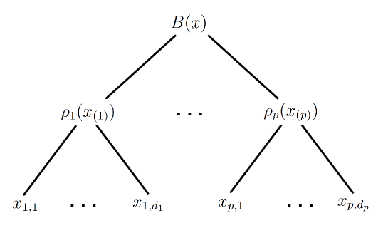
Figure 3: An interpretation of the semi-norm $B(\cdot)$ based on a tree

Tree structure provides useful information for doing grouping at different levels/depths. Theoretically, grouping allows us to detect a wider range of alternatives. For example, in two-sample testing, the difference between two one-dimensional marginals is always captured by the difference between two higher dimensional marginals that contain the two one-dimensional marginals. The same thing is true for dependence testing. Generally, one would like to find blocks which are nearly independent, but the variables inside a block have significant dependence among themselves. It is interesting to develop an algorithm for finding the optimal groups using the data and perhaps some auxiliary information. Another interesting direction is to study the semi-norm and distance constructed based on a more sophisticated tree structure. For example, in microbiome-wide association studies, phylogenetic tree or evolutionary tree which is a branching diagram or “tree” showing the evolutionary relationships among various biological species. Distance and kernel-based metrics constructed based on the distance utilizing the phylogenetic tree information is expected to be more powerful in signal detection. We leave these topics for future investigation.

Supplement to “A New Framework for Distance and Kernel-based Metrics in High Dimensions”
Shubhadeep Chakraborty
Department of Statistics, Texas A&M University
and
Xianyang Zhang
Department of Statistics, Texas A&M University

The supplement is organized as follows. In Section we explore our proposed homogeneity and dependence metrics in the low-dimensional setup. In Section we study the asymptotic behavior of our proposed homogeneity and dependence metrics in the high dimension medium sample size (HDMSS) framework where both the dimension(s) and the sample size(s) grow. Section illustrates an additional real data example for testing for independence in the high-dimensional framework. Finally, Section contains additional proofs of the main results in the paper and Sections and in the supplement.

Low-dimensional setup

In this section we illustrate that the new class of homogeneity metrics proposed in this paper inherits all the nice properties of generalized energy distance and MMD in the low-dimensional setting. Likewise, the proposed dependence metrics inherit all the desirable properties of generalized dCov and HSIC in the low-dimensional framework.

.1 Homogeneity metrics

Note that in either Case S1 or S2, the Euclidean space equipped with distance $K$ is of strong negative type. As a consequence, we have the following result.

Theorem .1.

$\mathcal{E}(X,Y)=0$ if and only if $X\overset{d}{=}Y$, in other words $\mathcal{E}(X,Y)$ completely characterizes the homogeneity of the distributions of $X$ and $Y$.

The following proposition shows that $\mathcal{E}_{n,m}(X,Y)$ is a two-sample U-statistic and an unbiased estimator of $\mathcal{E}(X,Y)$.

Proposition .1.

The U-statistic type estimator enjoys the following properties:

1. $\mathcal{E}_{n,m}$ is an unbiased estimator of the population $\mathcal{E}$.

2. $\mathcal{E}_{n,m}$ admits the following form :

   $$\mathcal{E}_{n,m}(X,Y)\;=\;\frac{1}{\binom{n}{2}\,\binom{m}{2}}\displaystyle\sum_{1\leq i<j\leq n}\,\sum_{1\leq k<l\leq m}h(X_{i},X_{j};Y_{k},Y_{l})\,,$$

   where

   $$h(X_{i},X_{j};Y_{k},Y_{l})\;=\;\frac{1}{2}\Big{(}K(X_{i},Y_{k})\,+\,K(X_{i},Y_{l})\,+\,K(X_{j},Y_{k})\,+\,K(X_{j},Y_{l})\Big{)}\,-\,K(X_{i},X_{j})\,-\,K(Y_{k},Y_{l})\,.$$

The following theorem shows the asymptotic behavior of the U-statistic type estimator of $\mathcal{E}$ for fixed $p$ and growing $n$.

Theorem .2.

Under Assumption 4.5 and the assumption that $\sup_{1\leq i\leq p}\mathbb{E}\rho_{i}(X_{(i)},0_{d_{i}})<\infty$ and $\sup_{1\leq i\leq p}\mathbb{E}\rho_{i}(Y_{(i)},0_{d_{i}})<\infty$, as $m,n\to\infty$ with $p$ remaining fixed, we have the following:

1. $\mathcal{E}_{n,m}(X,Y)\,\overset{a.s.}{\longrightarrow}\,\mathcal{E}(X,Y)$.

2. When $X\overset{d}{=}Y$, $\mathcal{E}_{n,m}$ has degeneracy of order $(1,1)$, and

   $$\frac{(m-1)(n-1)}{n+m}\,\mathcal{E}_{n,m}(X,Y)\,\overset{d}{\longrightarrow}\,\sum_{k=1}^{\infty}\lambda_{k}^{2}\left(Z_{k}^{2}\,-\,1\right)\,,$$

   where $\{Z_{k}\}$ is a sequence of independent $N(0,1)$ random variables and $\lambda_{k}$’s depend on the distribution of $(X,Y)$.

Proposition .1, Theorem .1 and Theorem .2 demonstrate that $\mathcal{E}$ inherits all the nice properties of generalized energy distance and MMD in the low-dimensional setting.

.2 Dependence metrics

Note that Proposition 3.1 in Section 3 and Proposition 3.7 in Lyons (2013) ensure that $\mathcal{D}(X,Y)$ completely characterizes independence between $X$ and $Y$, which leads to the following result.

Theorem .3.

Under Assumption 5.1, $\mathcal{D}(X,Y)=0$ if and only if $X\mathrel{\text{\scalebox{1.07}{$\perp\mkern-10.0mu\perp$}}}Y$.

The following proposition shows that $\widetilde{\mathcal{D}^{2}_{n}}(X,Y)$ is an unbiased estimator of $\mathcal{D}^{2}(X,Y)$ and is a U-statistic of order four.

Proposition .2.

The U-statistic type estimator $\widetilde{\mathcal{D}^{2}_{n}}$ (defined in (14) in the main paper) has the following properties:

1. $\widetilde{\mathcal{D}^{2}_{n}}$ is an unbiased estimator of the squared population $\mathcal{D}^{2}$.

2. $\widetilde{\mathcal{D}^{2}_{n}}$ is a fourth-order U-statistic which admits the following form:

   $$\widetilde{\mathcal{D}^{2}_{n}}\;=\;\frac{1}{\binom{n}{4}}\displaystyle\sum_{i<j<k<l}h_{i,j,k,l}\,,$$

   where

   $$h_{i,j,k,l}\, =\,\frac{1}{4!}\displaystyle\sum_{(s,t,u,v)}^{(i,j,k,l)}(d^{X}_{st}d^{Y}_{st}+d^{X}_{st}d^{Y}_{uv}-2d^{X}_{st}d^{Y}_{su})$$

   $$=\,\frac{1}{6}\displaystyle\sum_{s<t,u<v}^{(i,j,k,l)}(d^{X}_{st}d^{Y}_{st}+d^{X}_{st}d^{Y}_{uv})-\frac{1}{12}\displaystyle\sum_{(s,t,u)}^{(i,j,k,l)}d^{X}_{st}d^{Y}_{su}\,,$$

   the summation is over all possible permutations of the $4$-tuple of indices $(i,j,k,l)$. For example, when $(i,j,k,l)=(1,2,3,4)$, there exist 24 permutations, including $(1,2,3,4),\dots,(4,3,2,1)$. Furthermore, $\widetilde{\mathcal{D}^{2}_{n}}$ has degeneracy of order 1 when $X$ and $Y$ are independent.

The following theorem shows the asymptotic behavior of the U-statistic type estimator of $\mathcal{D}^{2}$ for fixed $p,q$ and growing $n$.

Theorem .4.

Under Assumption 5.1, with fixed $p,q$ and $n\to\infty$, we have the following as $n\to\infty$:

1. $\widetilde{\mathcal{D}^{2}_{n}}(X,Y)\overset{a.s.}{\longrightarrow}\mathcal{D}^{2}(X,Y)$;

2. When $\mathcal{D}^{2}(X,Y)=0$ (i.e., $X\mathrel{\text{\scalebox{1.07}{$\perp\mkern-10.0mu\perp$}}}Y$), $n\,\widetilde{\mathcal{D}^{2}_{n}}(X,Y)\,\overset{d}{\longrightarrow}\displaystyle\sum_{i=1}^{\infty}\tilde{\lambda}^{2}_{i}(Z_{i}^{2}-1)$,  where $Z_{i}^{\prime}s$ are i.i.d. standard normal random variables and  $\tilde{\lambda}_{i}$’s depend on the distribution of $(X,Y)$;

3. When $\mathcal{D}^{2}(X,Y)>0$, $n\,\widetilde{\mathcal{D}^{2}_{n}}(X,Y)\,\overset{a.s.}{\longrightarrow}\infty$.

Proposition .2, Theorem .3 and Theorem .4   demonstrate that in the low-dimensional setting, $\mathcal{D}$ inherits all the nice properties of generalized dCov and HSIC.

High dimension medium sample size (HDMSS)

.1 Homogeneity metrics

In this subsection, we consider the HDMSS setting where $p\to\infty$ and $n,m\to\infty$ at a slower rate than $p$. Under $H_{0}$, we impose the following conditions to obtain the asymptotic null distribution of the statistic $T_{n,m}$ under the HDMSS setup.

Assumption .1.

As $n,m$ and $p\to\infty$,

$$\frac{1}{n^{2}}\,\frac{\mathbb{E}\,\left[H^{4}(X,X^{\prime})\right]}{\left(\mathbb{E}\,\left[H^{2}(X,X^{\prime})\right]\right)^{2}}\;=\;o(1),\quad\frac{1}{n}\,\frac{\mathbb{E}\,\left[H^{2}(X,X^{\prime\prime})\,H^{2}(X^{\prime},X^{\prime\prime})\right]}{\left(\mathbb{E}\,\left[H^{2}(X,X^{\prime})\right]\right)^{2}}\;=\;o(1),$$

$$\frac{\mathbb{E}\,\left[H(X,X^{\prime\prime})\,H(X^{\prime},X^{\prime\prime})\,H(X,X^{\prime\prime\prime})\,H(X^{\prime},X^{\prime\prime\prime})\right]}{\left(\mathbb{E}\,\left[H^{2}(X,X^{\prime})\right]\right)^{2}}\;=\;o(1).$$

Remark .1.

We refer the reader to Section 2.2 in Zhang et al. (2018) and Remark A.2.2 in Zhu et al. (2019) for illustrations of Assumption .1 where $\rho_{i}$ has been considered to be the Euclidean distance or the squared Euclidean distance, respectively, for $1\leq i\leq p$.

Assumption .2.

Suppose $\mathbb{E}\,[L^{2}(X,X^{\prime})]=O(\alpha_{p}^{2})$ where $\alpha_{p}$ is a positive real sequence such that $\tau_{X}\alpha_{p}^{2}=o(1)$ as $p\to\infty$. Further assume that as  $n,p\to\infty$,

$$\frac{n^{4}\,\tau_{X}^{4}\,\mathbb{E}\,\left[R^{4}(X,X^{\prime})\right]}{\left(\mathbb{E}\,\left[H^{2}(X,X^{\prime})\right]\right)^{2}}=o(1)\,.$$

Remark .2.

We refer the reader to Remark 4.1 in the main paper which illustrates some sufficient conditions under which  $\alpha_{p}=O(\frac{1}{\sqrt{p}})$  and consequently  $\tau_{X}\alpha_{p}^{2}=o(1)$ holds, as  $\tau_{X}\asymp p^{1/2}$. In similar lines of Remark .1 in Section of the supplementary material, it can be argued that  $\mathbb{E}\,\left[R^{4}(X,X^{\prime})\right]=O\left(\frac{1}{p^{4}}\right)$. If we further assume that Assumption 4.4 holds, then we have $\mathbb{E}\,\left[H^{2}(X,X^{\prime})\right]\asymp 1$. Combining all the above, it is easy to verify that  $\frac{n^{4}\,\tau_{X}^{4}\,\mathbb{E}\,\left[R^{4}(X,X^{\prime})\right]}{\left(\mathbb{E}\,\left[H^{2}(X,X^{\prime})\right]\right)^{2}}=o(1)$  holds provided  $n=o(p^{1/2})$.

The following theorem illustrates the limiting null distribution of $T_{n,m}$ under the HDMSS setup. We refer the reader to Section of the supplement for a detailed proof.

Theorem .1.

Under $H_{0}$ and Assumptions 4.5, .1 and .2, as $n,m$ and $p\to\infty$, we have

$$T_{n,m}\;\overset{d}{\longrightarrow}\;N(0,1).$$

.2 Dependence metrics

In this subsection, we consider the HDMSS setting where $p,q\to\infty$ and $n\to\infty$ at a slower rate than $p,q$. The following theorem shows that similar to the HDLSS setting, under the HDMSS setup, $\widetilde{\mathcal{D}^{2}_{n}}$ is asymptotically equivalent to the aggregation of group-wise generalized dCov. In other words $\widetilde{\mathcal{D}^{2}_{n}}(X,Y)$ can quantify group-wise nonlinear dependence between $X$ and $Y$ in the HDMSS setup as well.

Assumption .3.

$\mathbb{E}[L_{X}(X,X^{\prime})^{2}]=\alpha_{p}^{2}$, $\mathbb{E}[L_{X}(X,X^{\prime})^{4}]=\gamma_{p}^{2}$, $\mathbb{E}[L_{Y}(Y,Y^{\prime})^{2}]=\beta_{q}^{2}$ and $\mathbb{E}[L_{Y}(Y,Y^{\prime})^{4}]=\lambda_{q}^{2}$, where $\alpha_{p},\gamma_{p},\beta_{q},\lambda_{q}$ are positive real sequences satisfying $n\alpha_{p}=o(1)$, $n\beta_{q}=o(1)$, $\tau_{X}^{2}(\alpha_{p}\gamma_{p}+\gamma_{p}^{2})=o(1)$, $\tau_{Y}^{2}(\beta_{q}\lambda_{q}+\lambda_{q}^{2})=o(1)$, and  $\tau_{XY}\,(\alpha_{p}\lambda_{q}+\gamma_{p}\beta_{q}+\gamma_{p}\lambda_{q})=o(1)$.

Remark .3.

Following Remark 4.1 in the main paper, we can write   $L(X,X^{\prime})=O(\frac{1}{p})\sum_{i=1}^{p}\left(Z_{i}-\mathbb{E}\,Z_{i}\right)$, where $Z_{i}=\rho_{i}(X_{(i)},X_{(i)}^{\prime})$ for $1\leq i\leq p$. Assume that $\sup_{1\leq i\leq p}\mathbb{E}\,\rho_{i}^{4}(X_{(i)},0_{d_{i}})<\infty$, which implies  $\sup_{1\leq i\leq p}\mathbb{E}\,Z_{i}^{4}<\infty$. Under certain weak dependence assumptions, it can be shown that  $\mathbb{E}\,\big{(}\sum_{i=1}^{p}(Z_{i}-\mathbb{E}\,Z_{i})\big{)}^{4}=O(p^{2})$ as $p\to\infty$ (see for example Theorem 1 in Doukhan et al. (1999)). Therefore we have  $\mathbb{E}[L(X,X^{\prime})^{4}]=O(\frac{1}{p^{2}})$. It follows from Hölder’s inequality that  $\mathbb{E}[L(X,X^{\prime})^{2}]=O(\frac{1}{p})$. Similar arguments can be made about  $\mathbb{E}[L(Y,Y^{\prime})^{4}]$ and $\mathbb{E}[L(Y,Y^{\prime})^{2}]$ as well.

Theorem .2.

Under Assumptions 4.2 and .3, we can show that

$$\widetilde{\mathcal{D}^{2}_{n}}(X,Y)=\frac{1}{4\tau_{XY}}\displaystyle\sum_{i=1}^{p}\sum_{j=1}^{q}\widetilde{D^{2}_{n}}_{\,;\,\rho_{i},\rho_{j}}(X_{(i)},Y_{(j)})\,+\,\mathcal{R}_{n}\;,$$ (40)

where $\mathcal{R}_{n}$ is the remainder term satisfying that $\mathcal{R}_{n}=O_{p}(\tau_{XY}\,(\alpha_{p}\lambda_{q}+\gamma_{p}\beta_{q}+\gamma_{p}\lambda_{q}))=o_{p}(1)$, i.e., $\mathcal{R}_{n}$ is of smaller order compared to the leading term and hence is asymptotically negligible.

The following theorem states the asymptotic null distribution of the studentized test statistic $\mathcal{T}_{n}$ (given in equation (39) in the main paper) under the HDMSS setup. Define

$$U(X_{k},X_{l}):=\frac{1}{\tau_{X}}\displaystyle\sum_{i=1}^{p}d^{X}_{kl}(i),\quad\text{and}\quad V(Y_{k},Y_{l}):=\frac{1}{\tau_{Y}}\displaystyle\sum_{i=1}^{q}d^{Y}_{kl}(i).$$

Assumption .4.

Assume that

$$\frac{\mathbb{E}\left[U(X,X^{\prime})\right]^{4}}{\sqrt{n}\left(\mathbb{E}[U(X,X^{\prime})]^{2}\right)^{2}}\,=\,o(1),$$

$$\frac{\mathbb{E}\left[U(X,X^{\prime})\,U(X^{\prime},X^{\prime\prime})\,U(X^{\prime\prime},X^{\prime\prime\prime})\,U(X^{\prime\prime\prime},X)\right]}{\left(\mathbb{E}[U(X,X^{\prime})]^{2}\right)^{2}}\,=\,o(1),$$

and the same conditions hold for $Y$ in terms of $V(Y,Y^{\prime})$.

Remark .4.

We refer the reader to Section 2.2 in Zhang et al. (2018) and Remark A.2.2 in Zhu et al. (2019) for illustrations of Assumption .1 where $\rho_{i}$ has been considered to be the Euclidean distance or the squared Euclidean distance, respectively.

We can show that under $H_{0}$, the studentized test $\mathcal{T}_{n}$ converge to the standard normal distribution under the HDMSS setup.

Theorem .3.

Under $H_{0}$ and Assumptions .3-.4, as $n,p,q\to\infty$, we have  $\mathcal{T}_{n}\,\overset{d}{\longrightarrow}\,N(0,1)\,.$

Additional real data example

We consider the monthly closed stock prices of $\tilde{p}=33$ companies under the oil and gas sector and $\tilde{q}=34$ companies under the transport sector between January 1, 2017 and December 31, 2018. The companies under both the sectors are clustered or grouped according to their countries. The data has been downloaded from Yahoo Finance via the R package ‘quantmod’. Under the oil and gas sector, we have $p=18$ countries or groups, viz. USA, Australia, UK, Canada, China, Singapore, Hong Kong, Netherlands, Colombia, Italy, Norway, Bermuda, Switzerland, Brazil, South Africa, France, Turkey and Argentina, with $d=(5,1,2,5,4,1,1,2,1,1,1,1,2,1,1,2,1,1)$. And under the transport sector, we have $q=14$ countries or groups, viz. USA, Brazil, Canada, Greece, China, Panama, Belgium, Bermuda, UK, Mexico, Chile, Monaco, Ireland and Hong Kong, with $g=(5,1,2,6,4,1,1,3,1,3,1,4,1,1)$. At each time $t$, denote the closed stock prices of these companies from the two different sectors by $X_{t}=(X_{1t},\dots,X_{pt})$ and $Y_{t}=(Y_{1t},\dots,Y_{qt})$ for $1\leq t\leq 24$. We consider the stock returns $S^{X}_{t}=(S^{X}_{1t},\dots,S^{X}_{pt})$ and $S^{Y}_{t}=(S^{Y}_{1t},\dots,S^{Y}_{qt})$ for $1\leq t\leq 23$, where $S^{X}_{itl}=\log\frac{X_{i,t+1,l}}{X_{itl}}$ and $S^{Y}_{jtl^{\prime}}=\log\frac{Y_{j,t+1,l^{\prime}}}{Y_{jtl^{\prime}}}$ for $1\leq l\leq d_{i}$, $1\leq i\leq p$, $1\leq l^{\prime}\leq g_{j}$ and $1\leq j\leq q$.

The intuitive idea is, stock returns of oil and gas companies should affect the stock returns of companies under the transport sector, and here both the random vectors admit a natural grouping based on the countries. Table 9 shows the p-values corresponding to the different tests for independence between $\{S^{X}_{t}\}_{t=1}^{23}$ and $\{S^{Y}_{t}\}_{t=1}^{23}$. The tests based on the proposed dependence metrics considering the natural grouping deliver much smaller p-values compared to the tests based on the usual dCov and HSIC which fail to reject the null hypothesis of independence between $\{S^{X}_{t}\}_{t=1}^{23}$ and $\{S^{Y}_{t}\}_{t=1}^{23}$. This makes intuitive sense as the dependence among financial asset returns is usually nonlinear in nature and thus cannot be fully characterized by the usual dCov and HSIC in the high dimensional setup.

Table 9: p-values corresponding to the different tests for cross-sector independence of stock returns data considering the natural grouping based on countries.

I	II	III	IV	V	VI
$0.036$	$0.048$	$0.087$	$0.247$	$0.136$	$0.281$

Table 10 shows the p-values corresponding to the different tests for independence when we disregard the natural grouping and consider $d_{i}=1$ and $g_{j}=1$ for all $1\leq i\leq p$ and $1\leq j\leq q$. Considering unit group sizes makes our proposed statistics essentially equivalent to the marginal aggregation approach proposed by Zhu et al. (2019). In this case the proposed tests have higher p-values than when we consider the natural grouping, indicating that grouping or clustering might improve the power of testing as they are capable of detecting a wider range of dependencies.

Table 10: p-values corresponding to the different tests for cross-sector independence of stock returns data considering unit group sizes.

I	II	III	IV	V	VI
$0.092$	$0.209$	$0.226$	$0.247$	$0.136$	$0.281$

Technical Appendix

Proof of Proposition 3.1.

To prove (1), note that if $d$ is a metric on a space $\mathcal{X}$, then so is $d^{1/2}$. It is easy to see that $K^{2}$ is a metric on $\mathbb{R}^{\tilde{p}}$. To prove (2), note that $(\mathbb{R}^{d_{i}},\rho_{i})$ has strong negative type for $1\leq i\leq p$. The rest follows from Corollary 3.20 in Lyons (2013). $\diamondsuit$

Proof of Proposition .1.

It is easy to verify that $\mathcal{E}_{n,m}$ is an unbiased estimator of $\mathcal{E}$ and is a two-sample U-statistic with the kernel $h$. $\diamondsuit$

Proof of Theorem .2.

The first part of the proof follows from Theorem 1 in Sen (1977) and the observation that $\mathbb{E}\,\left[|h|\log^{+}|h|\right]\leq\mathbb{E}[h^{2}]$. The power mean inequality says that for  $a_{i}\in\mathbb{R},\,1\leq i\leq n,\,n\geq 2$ and $r>1$,

$$\left|\displaystyle\sum_{i=1}^{n}a_{i}\right|^{r}\;\leq\;n^{r-1}\,\displaystyle\sum_{i=1}^{n}|a_{i}|^{r}\,.$$ (41)

Using the power mean inequality, it is easy to see that the assumptions $\sup_{1\leq i\leq p}\mathbb{E}\rho_{i}(X_{(i)},0_{d_{i}})<\infty$ and $\sup_{1\leq i\leq p}\mathbb{E}\rho_{i}(Y_{(i)},0_{d_{i}})<\infty$ ensure that $\mathbb{E}[h^{2}]<\infty$. For proving the second part, define $h_{1,0}(X)=\;\mathbb{E}\,\left[h(X,X^{\prime};Y,Y^{\prime})|X\right]$ and $h_{0,1}(Y)=\;\mathbb{E}\,\left[h(X,X^{\prime};Y,Y^{\prime})|Y\right]$ Clearly, when $X\overset{d}{=}Y$, $h_{1,0}(X)$ and $h_{0,1}(Y)$ are degenerate at $0$ almost surely. Following Theorem 1.1 in Neuhaus (1977), we have

$$\frac{(m-1)(n-1)}{n+m}\,\mathcal{E}_{nm}(X,Y)\,\overset{d}{\longrightarrow}\,\sum_{k=1}^{\infty}\sigma_{k}^{2}\left[(a_{k}U_{k}+b_{k}V_{k})^{2}\,-\,(a_{k}^{2}+b_{k}^{2})\right]\,,$$

where $\{U_{k}\},\{V_{k}\}$ are two sequences of independent $N(0,1)$ variables, independent of each other, and $(\sigma_{k},a_{k},b_{k})$’s depend on the distribution of $(X,Y)$. The proof can be completed by some simple rearrangement of terms. $\diamondsuit$

Proof of Proposition 4.1.

The proof is essentially similar to the proof of Proposition 2.1.1 in Zhu et al. (2019), replacing the Euclidean distance between, for example, $X$ and $X^{\prime}$, viz. $\|X-X^{\prime}\|_{\tilde{p}}$ , by the new distance metric $K(X,X^{\prime})$. To show that $R(X,X^{\prime})=O_{p}(L^{2}(X,X^{\prime}))$ if $L(X,X^{\prime})=o_{p}(1)$, we define $f(x)=\sqrt{1+x}$. By the definition of the Lagrange’s form of the remainder term from Taylor’s expansion, we have

$$R(X,X^{\prime})=\int_{0}^{L(X,X^{\prime})}f^{\prime\prime}(t)\left(\,L(X,X^{\prime})-t\,\right)\,dt\,.$$

Using $R$ and $L$ interchangeably with $R(X,X^{\prime})$ and $L(X,X^{\prime})$ respectively, we can write

$$\begin{split}|R|\;&\leq\;|L|\,\left[\int_{0}^{L}f^{\prime\prime}(t)\,\mathbbm{1}_{L>0}\,dt\;+\;\int_{L}^{0}f^{\prime\prime}(t)\,\mathbbm{1}_{L<0}\,dt\,\right]\\ &=\;\frac{|L|}{2}\,\big{|}1-\frac{1}{\sqrt{1+L}}\big{|}\\ &=\;\frac{|L|}{2}\,\frac{|L|}{1+L+\sqrt{1+L}}\\ &\leq\;\frac{L^{2}}{2(1+L)}\,.\end{split}$$ (42)

It is clear that $R(X,X^{\prime})=O_{p}(L^{2}(X,X^{\prime}))$ provided that $L(X,X^{\prime})=o_{p}(1)$. $\diamondsuit$

Proof of Theorem 4.1.

Observe that $\mathbb{E}\,L(X,Y)=\mathbb{E}\,L(X,X^{\prime})=\mathbb{E}\,L(Y,Y^{\prime})=0$. By Proposition 4.1,

$$\mathcal{E}(X,Y)\; =\;2\,\mathbb{E}\,\left[\tau+\tau\,R(X,Y)\right]\,-\,\mathbb{E}\,\left[\tau_{X}+\tau_{X}\,R(X,X^{\prime})\right]\,-\,\mathbb{E}\,\left[\tau_{Y}+\tau_{Y}\,R(Y,Y^{\prime})\right]$$

$$=\;2\tau-\tau_{X}-\tau_{Y}\,+\,\mathcal{R}_{\mathcal{E}}\,.$$

Clearly $|\mathcal{R}_{\mathcal{E}}|\;\leq\;2\,\tau\,\mathbb{E}\,\left[\,|R(X,Y)|\,\right]\,+\,\tau_{X}\,\mathbb{E}\,\left[\,|R(X,X^{\prime})|\,\right]\,+\,\tau_{Y}\,\mathbb{E}\,\left[\,|R(Y,Y^{\prime})|\,\right].$ By (42) and Assumption 4.3, we have

$$\tau|R(X,Y)|\leq\frac{\tau L^{2}(X,Y)}{2(1+L(X,Y))}=O(\tau a^{2}_{p})=o_{p}(1).$$

As $\{\sqrt{p}L^{2}(X,Y)/(1+L(X,Y))\}$ is uniformly integrable and $\tau\asymp\sqrt{p}$, we must have $\tau\mathbb{E}[|R(X,Y)|]=o(1)$. The other terms can be handled in a similar fashion. $\diamondsuit$

Remark .1.

Write $L(X,Y)=\frac{1}{\tau^{2}}(A_{p}-\mathbb{E}\,A_{p})=\frac{1}{\tau^{2}}\sum_{i=1}^{p}(Z_{i}-\mathbb{E}Z_{i})$, where $A_{p}:=\sum_{i=1}^{p}Z_{i}$ and $Z_{i}:=\rho_{i}(X_{i},Y_{i})$ for $1\leq i\leq p$. Assume $\sup_{i}\mathbb{E}\rho_{i}^{8}(X_{i},0_{d_{i}})<\infty$ and  $\sup_{i}\mathbb{E}\rho_{i}^{8}(X_{i},0_{d_{i}})<\infty$, which imply $\sup_{i}\mathbb{E}Z_{i}^{8}<\infty$. Denote $L(X,Y)$ by $L$ and $R(X,Y)$ by $R$ for notational simplicities. Further assume that $E\exp(tA_{p})=O((1-\theta_{1}t)^{-\theta_{2}p})$ for $\theta_{1},\theta_{2}>0$ and $\theta_{2}\,p>4$ uniformly over  $t<0$ (which is clearly satisfied when $Z_{i}$’s are independent and $\mathbb{E}\exp(tZ_{i})\leq a_{1}(1-a_{2}t)^{-a_{3}}$ uniformly over $t<0$ and   $1\leq i\leq p$ for some $a_{1},a_{2},a_{3}>0$ with $a_{3}\,p>4$). Under certain weak dependence assumptions, it can be shown that:

1. $\{\sqrt{p}L^{2}/(1+L)\}$ is uniformly integrable;

2. $\mathbb{E}\,R^{2}=O(\frac{1}{p^{2}})$.

Similar arguments hold for $L(X,X^{\prime})$ and $R(X,X^{\prime})$, and, $L(Y,Y^{\prime})$ and $R(Y,Y^{\prime})$ as well.

Proof of Remark .1.

To prove the first part, define $L_{p}:=\sqrt{p}L^{2}/(1+L)$. Following Chapter 6 of Resnick (1999), it suffices to show that $\sup_{p}\mathbb{E}\,L_{p}^{2}<\infty$. Towards that end, using Hölder’s inequality we observe

$$\mathbb{E}\,L_{p}^{2}\; \leq\left(\mathbb{E}(p^{2}L^{8})\right)^{1/2}\,\left(\mathbb{E}\Big{[}\frac{1}{(1+L)^{4}}\Big{]}\right)^{1/2}\,.$$ (43)

With $\sup_{i}\mathbb{E}Z_{i}^{8}<\infty$ and under certain weak dependence assumptions, it can be shown that $\mathbb{E}(A_{p}-\mathbb{E}A_{p})^{8}=O(p^{4})$ (see for example Theorem 1 in Doukhan et al. (1999)). Consequently we have $\mathbb{E}\,L^{8}=O(\frac{1}{p^{4}})$ , as $\tau\asymp\sqrt{p}$. Clearly this yields  $\mathbb{E}\,(p^{2}L^{8})=O(\frac{1}{p^{2}})$.

Now note that

$$\mathbb{E}\Big{[}\frac{1}{(1+L)^{4}}\Big{]}\; =\;\tau^{8}\,\mathbb{E}\left(\frac{1}{A_{p}^{4}}\right)\,.$$ (44)

Equation (3) in Cressie et al. (1981) states that for a non-negative random variable $U$ with moment-generating function $M_{U}(t)=\mathbb{E}\exp(tU)$, one can write

$$\mathbb{E}(U^{-k}) =(\Gamma(k))^{-1}\displaystyle\int_{0}^{\infty}t^{k-1}M_{U}(-t)\,dt\,,$$ (45)

for any positive integer $k$, provided both the integrals exist. Using equation (45), the assumptions stated in Remark .1 and basic properties of beta integrals, some straightforward calculations yield

$$\mathbb{E}\left(\frac{1}{A_{p}^{4}}\right)\; \leq\;C_{1}\,\int_{0}^{\infty}\frac{t^{4-1}}{(1+\theta_{1}t)^{\theta_{2}p}}\,dt\;=\;C_{2}\,\frac{\Gamma(\theta_{2}p-4)}{\Gamma(\theta_{2}p)}\,,$$ (46)

where $C_{1},C_{2}$ are positive constants, which clearly implies that $\mathbb{E}\left(\frac{1}{A_{p}^{4}}\right)=O(\frac{1}{p^{4}})$. This together with equation (44) implies that $\mathbb{E}\Big{[}\frac{1}{(1+L)^{4}}\Big{]}=O(1)$, as $\tau\asymp\sqrt{p}$.

Combining all the above, we get from (43) that $\mathbb{E}\,L_{p}^{2}=O(\frac{1}{p})$ and therefore $\sup_{p}\mathbb{E}\,L_{p}^{2}<\infty$, which completes the proof of the first part.

To prove the second part, note that following the proof of Proposition 4.1 and Hölder’s inequality we can write

$$\mathbb{E}\,R^{2}=O\left(\mathbb{E}\,\left[\frac{L^{4}}{(1+L)^{2}}\right]\right)=O\left(\left(\mathbb{E}(L^{8})\right)^{1/2}\,\left(\mathbb{E}\Big{[}\frac{1}{(1+L)^{4}}\Big{]}\right)^{1/2}\right)\,.$$ (47)

Following the arguments as in the proof of the first part, clearly we have $\mathbb{E}\,L^{8}=O(\frac{1}{p^{4}})$ and $\mathbb{E}\Big{[}\frac{1}{(1+L)^{4}}\Big{]}=O(1)$. From this and equation (47), it is straightforward to verify that $\mathbb{E}\,R^{2}=O(\frac{1}{p^{2}})$, which completes the proof of the second part. $\diamondsuit$

Proof of Lemma 4.1.

To see (2), first observe that the sufficient part is straightforward from equation (21) in the main paper. For the necessary part, denote $a=\textrm{tr}\,\Sigma_{X}$, $b=\textrm{tr}\,\Sigma_{Y}$ and $c=\|\mu_{X}-\mu_{Y}\|^{2}$. Then we have $2\,\sqrt{a+b+c}=\sqrt{2a}+\sqrt{2b}$. Some straightforward calculations yield $(\sqrt{2a}-\sqrt{2b})^{2}+4\,c=0$ which implies the rest.

To see (1), again the sufficient part is straightforward from equation (20) in the paper and the form of $K$ given in equation (15) in the paper. For the necessary part, first note that as $(\mathbb{R}^{d_{i}},\rho_{i})$ is a metric space of strong negative type for $1\leq i\leq p$, there exists a Hilbert space $\mathcal{H}_{i}$ and an injective map $\phi_{i}:\mathbb{R}^{d_{i}}\to\mathcal{H}_{i}$ such that $\rho_{i}(z,z^{\prime})=\|\phi_{i}(z)-\phi_{i}(z^{\prime})\|^{2}_{\mathcal{H}_{i}}$ , where $\langle\cdot,\cdot\rangle_{\mathcal{H}_{i}}$ is the inner product defined on $\mathcal{H}_{i}$ and $\|\cdot\|_{\mathcal{H}_{i}}$ is the norm induced by the inner product (see Proposition 3 in Sejdinovic et al. (2013) for detailed discussions). Further, if $k_{i}$ is a distance-induced kernel induced by the metric $\rho_{i}$, then by Proposition 14 in Sejdinovic et al. (2013), $\mathcal{H}_{i}$ is the RKHS with the reproducing kernel $k_{i}$ and $\phi_{i}(z)$ is essentially the canonical feature map for $\mathcal{H}_{i}$, viz. $\phi_{i}(z):z\mapsto k_{i}(\cdot,z)$. It is easy to see that

$$\tau_{X}^{2}\,= \,\mathbb{E}\,\sum^{p}_{i=1}\|\phi_{i}(X_{(i)})-\phi_{i}(X_{(i)}^{\prime})\|^{2}_{\mathcal{H}_{i}}\,=\,2\,\mathbb{E}\sum^{p}_{i=1}\|\phi_{i}(X_{(i)})-\mathbb{E}\,\phi_{i}(X_{(i)})\|^{2}_{\mathcal{H}_{i}},$$

$$\tau_{Y}^{2}\,= \,\mathbb{E}\,\sum^{p}_{i=1}\|\phi_{i}(Y_{(i)})-\phi_{i}(Y_{(i)}^{\prime})\|^{2}_{\mathcal{H}_{i}}\,=\,2\,\mathbb{E}\sum^{p}_{i=1}\|\phi_{i}(Y_{(i)})-\mathbb{E}\,\phi_{i}(Y_{(i)})\|^{2}_{\mathcal{H}_{i}},$$

$$\tau^{2}\,= \,\mathbb{E}\,\sum^{p}_{i=1}\|\phi_{i}(X_{(i)})-\phi_{i}(Y_{(i)})\|^{2}_{\mathcal{H}_{i}}\,=\,\tau_{X}^{2}/2+\tau_{Y}^{2}/2+\zeta^{2},$$

where $\zeta^{2}=\sum^{p}_{i=1}\|\mathbb{E}\,\phi(X_{(i)})-\mathbb{E}\,\phi(Y_{(i)})\|^{2}_{\mathcal{H}_{i}}$. Thus $2\tau-\tau_{X}-\tau_{Y}=0$  is equivalent to

$$4(\tau_{X}^{2}/2+\tau_{Y}^{2}/2+\zeta^{2})=(\tau_{X}+\tau_{Y})^{2}=\tau_{X}^{2}+\tau_{Y}^{2}+2\tau_{X}\tau_{Y}.$$

which implies that

$$4\zeta^{2}+(\tau_{X}-\tau_{Y})^{2}=0.$$

Therefore, $2\tau-\tau_{X}-\tau_{Y}=0$  holds if and only if (1) $\zeta=0$, i.e., $\mathbb{E}\,\phi_{i}(X_{(i)})=\mathbb{E}\,\phi_{i}(Y_{(i)})$ for all $1\leq i\leq p$, and, (2) $\tau_{X}=\tau_{Y}$, i.e.,

$$\mathbb{E}\sum^{p}_{i=1}\|\phi_{i}(X_{(i)})-\mathbb{E}\,\phi_{i}(X_{(i)})\|_{\mathcal{H}_{i}}^{2}\,=\,\mathbb{E}\sum^{p}_{i=1}\|\phi_{i}(Y_{(i)})-\mathbb{E}\,\phi_{i}(Y_{(i)})\|_{\mathcal{H}_{i}}^{2}.$$

Now if $X\sim P$ and $Y\sim Q$, then note that

$$\mathbb{E}\,\phi_{i}(X_{(i)})\,=\,\displaystyle\int_{\mathbb{R}^{d_{i}}}k_{i}(\cdot,z)\,dP_{i}(z)\,=\,\Pi_{i}(P_{i})\;\;\;\textrm{and}\;\;\;\mathbb{E}\,\phi_{i}(Y_{(i)})\,=\,\displaystyle\int_{\mathbb{R}^{d_{i}}}k_{i}(\cdot,z)\,dQ_{i}(z)\,=\,\Pi_{i}(Q_{i})\,,$$

where $\Pi_{i}$ is the mean embedding function (associated with the distance induced kernel $k_{i}$) defined in Section 2.1, $P_{i}$ and $Q_{i}$ are the distributions of $X_{(i)}$ and $Y_{(i)}$, respectively. As $\rho_{i}$ is a metric of strong negative type on $\mathbb{R}^{d_{i}}$, the induced kernel $k_{i}$ is characteristic to $\mathcal{M}_{1}(\mathbb{R}^{d_{i}})$ and hence the mean embedding function $\Pi_{i}$ is injective. Therefore condition (1) above implies $X_{(i)}\overset{d}{=}Y_{(i)}$. $\diamondsuit$

Now we introduce some notation before presenting the proof of Theorem 4.2. The key of our analysis is to study the variance of the leading term of $\mathcal{E}_{n,m}(X,Y)$ in the HDLSS setup, propose the variance estimator and study the asymptotic behavior of the variance estimator. It will be shown later (in the proof of Theorem 4.2) that the leading term in the Taylor’s expansion of $\mathcal{E}_{n,m}(X,Y)-(2\tau-\tau_{X}-\tau_{Y})$ can be written as $L_{1}+L_{2}$, where

$$\begin{split}L_{1}\;&:=\;\frac{1}{nm\tau}\sum_{k=1}^{n}\sum_{l=1}^{m}\sum_{i=1}^{p}d_{kl}(i)-\frac{1}{n(n-1)\tau_{X}}\sum_{k<l}\sum_{i=1}^{p}d^{X}_{kl}(i)-\frac{1}{m(m-1)\tau_{Y}}\sum_{k<l}\sum_{i=1}^{p}d^{Y}_{kl}(i)\\ \;&:=\,L_{1}^{1}-L_{1}^{2}-L_{1}^{3}\;,\end{split}$$ (48)

where $L_{1}^{i}$’s are defined accordingly and

$$\begin{split}L_{2}\;:=&\;\frac{1}{nm\tau}\sum_{k=1}^{n}\sum_{l=1}^{m}\sum_{i=1}^{p}\Big{(}\mathbb{E}\,[\rho_{i}(X_{k(i)},Y_{l(i)})|X_{k(i)}]+[\rho_{i}(X_{k(i)},Y_{l(i)})|Y_{l(i)}]-2\,\mathbb{E}\,\rho_{i}(X_{k(i)},Y_{l(i)})\Big{)}\\ &\;-\frac{1}{n(n-1)\tau_{X}}\sum_{k<l}\sum_{i=1}^{p}\Big{(}\mathbb{E}\,[\rho_{i}(X_{k(i)},X_{l(i)})|X_{k(i)}]+[\rho_{i}(X_{k(i)},X_{l(i)})|X_{l(i)}]-2\,\mathbb{E}\,\rho_{i}(X_{k(i)},X_{l(i)})\Big{)}\\ &-\frac{1}{m(m-1)\tau_{Y}}\sum_{k<l}\sum_{i=1}^{p}\Big{(}\mathbb{E}\,[\rho_{i}(Y_{k(i)},Y_{l(i)})|Y_{k(i)}]+[\rho_{i}(Y_{k(i)},Y_{l(i)})|Y_{l(i)}]-2\,\mathbb{E}\,\rho_{i}(Y_{k(i)},Y_{l(i)})\Big{)}\,.\end{split}$$ (49)

By the double-centering properties, it is easy to see that $L_{1}^{i}$ for $1\leq i\leq 3$ are uncorrelated. Define

$$\begin{split}V:=&\frac{1}{nm\tau^{2}}\sum_{i,i^{\prime}=1}^{p}\mathbb{E}\,[d_{kl}(i)\,d_{kl}(i^{\prime})]\;+\;\frac{1}{2n(n-1)\tau^{2}_{X}}\sum_{i,i^{\prime}=1}^{p}\mathbb{E}\,[d_{kl}^{X}(i)\,d_{kl}^{X}(i^{\prime})]\\ &+\;\frac{1}{2m(m-1)\tau^{2}_{Y}}\sum_{i,i^{\prime}=1}^{p}\mathbb{E}\,[d_{kl}^{Y}(i)\,d_{kl}^{Y}(i^{\prime})]\\ :=&\;V_{1}\;+\;V_{2}\;+\;V_{3},\end{split}$$ (50)

where $V_{i}$’s are defined accordingly. Further let

$$\widetilde{V_{1}}\;:=\;nmV_{1}\;,\;\widetilde{V_{2}}\;:=\;2n(n-1)V_{2}\;,\;\widetilde{V_{3}}\;:=\;2m(m-1)V_{3}\,.$$ (51)

It can be verified that

$$\mathbb{E}\,[d^{X}_{kl}(i)\,d^{X}_{kl}(i^{\prime})]\;=\;D^{2}_{\rho_{i},\rho_{i^{\prime}}}(X_{(i)},X_{(i^{\prime})})\,.$$

Thus we have

$$\widetilde{V_{2}}\;=\;\frac{1}{\tau^{2}_{X}}\displaystyle\sum_{i,i^{\prime}=1}^{p}D^{2}_{\rho_{i},\rho_{i^{\prime}}}(X_{(i)},X_{(i^{\prime})})\;\;\;\;\textrm{and}\;\;\;\;\widetilde{V_{3}}\;=\;\frac{1}{\tau^{2}_{Y}}\displaystyle\sum_{i,i^{\prime}=1}^{p}D^{2}_{\rho_{i},\rho_{i^{\prime}}}(Y_{(i)},Y_{(i^{\prime})})\,.$$ (52)

We study the variances of $L_{1}^{i}$ for $1\leq i\leq 3$ and propose some suitable estimators. The variance for $L_{1}^{2}$ is given by

$$var(L_{1}^{2})\;= \;\frac{1}{n^{2}(n-1)^{2}\tau_{X}^{2}}\sum_{i,i^{\prime}=1}^{p}\sum_{k<l}\mathbb{E}\,[d^{X}_{kl}(i)\,d^{X}_{kl}(i^{\prime})]\;=\;V_{2}\,.$$

Clearly

$$\frac{n(n-1)V_{2}}{2}\;=\;\frac{1}{4\tau^{2}_{X}}\displaystyle\sum_{i,i^{\prime}=1}^{p}D^{2}_{\rho_{i},\rho_{j}}(X_{(i)},X_{(i^{\prime})})\,.$$

From Theorem 5.3  in Section 5.1, we know that for fixed $n$ and growing $p$, $\widetilde{\mathcal{D}_{n}^{2}}(X,X)$ is asymptotically equivalent to $\frac{1}{4\tau^{2}_{X}}\sum_{i,i^{\prime}=1}^{p}\widetilde{D^{2}_{n}}_{\,;\,\rho_{i},\rho_{j}}(X_{(i)},X_{(i^{\prime})})$. Therefore an estimator of $\widetilde{V_{2}}$ is given by $4\,\widetilde{\mathcal{D}_{n}^{2}}(X,X)$. Note that the computational cost of $\widetilde{\mathcal{D}_{n}^{2}}(X,X)$ is linear in $p$ while direct calculation of its leading term $\frac{1}{4\tau^{2}_{X}}\sum_{i,i^{\prime}=1}^{p}\widetilde{D^{2}_{n}}_{\,;\,\rho_{i},\rho_{j}}(X_{(i)},X_{(i^{\prime})})$ requires computation in the quadratic order of $p$. Similarly it can be shown that the variance of $L_{1}^{3}$ is $V_{3}$ and $\widetilde{V_{3}}$ can be estimated by $4\,\widetilde{\mathcal{D}_{m}^{2}}(Y,Y)$. Likewise some easy calculations show that the variance of $L_{1}^{1}$ is $V_{1}$. Define

$$\begin{split}\hat{\rho_{i}}(X_{k(i)},Y_{l(i)})\;:=&\;\rho_{i}(X_{k(i)},Y_{l(i)})\,-\,\frac{1}{n}\sum^{n}_{a=1}\rho_{i}(X_{a(i)},Y_{l(i)})\,-\,\frac{1}{m}\sum^{m}_{b=1}\rho_{i}(X_{k(i)},Y_{b(i)})\\ &+\,\frac{1}{nm}\sum_{a=1}^{n}\sum^{m}_{b=1}\rho_{i}(X_{a(i)},Y_{b(i)})\;,\end{split}$$ (53)

and

$$\hat{R}(X_{k},Y_{l})\;:=\;R(X_{k},Y_{l})-\frac{1}{n}\sum^{n}_{a=1}R(X_{a},Y_{l})-\frac{1}{m}\sum^{m}_{b=1}R(X_{k},Y_{b})+\frac{1}{nm}\sum_{a=1}^{n}\sum^{m}_{b=1}R(X_{a},Y_{b})\,.$$ (54)

It can be verified that

$$\hat{\rho_{i}}(X_{k(i)},Y_{l(i)})\;=\;d_{kl}(i)\,-\,\frac{1}{n}\sum^{n}_{a=1}d_{al}(i)\,-\,\frac{1}{m}\sum^{m}_{b=1}d_{kb}(i)\,+\,\frac{1}{nm}\sum_{a=1}^{n}\sum^{m}_{b=1}d_{ab}(i).$$

Observe that

$$\mathbb{E}\,[\hat{\rho_{i}}(X_{k(i)},Y_{l(i)})\rho_{i^{\prime}}(X_{k(i^{\prime})},Y_{l(i^{\prime})})]\;=\;(1-1/n)(1-1/m)\,\mathbb{E}\,[d_{kl}(i)\,d_{kl}(i^{\prime})]\,.$$ (55)

Let $\hat{\bf A}_{i}=(\hat{\rho_{i}}(X_{k(i)},Y_{l(i)}))_{k,l},\;{\bf A}_{i}=(\rho_{i}(X_{k(i)},Y_{l(i)}))_{k,l}\,\in\mathbb{R}^{n\times m}$. Note that

$$\begin{split}&\;\frac{1}{(n-1)(m-1)}\,\mathbb{E}\,\sum_{k=1}^{n}\sum_{l=1}^{m}\hat{\rho_{i}}(X_{k(i)},Y_{l(i)})\hat{\rho_{i}}(X_{k(i^{\prime})},Y_{l(i^{\prime})})\\ =&\;\frac{1}{(n-1)(m-1)}\,\mathbb{E}\,\text{tr}(\hat{{\bf A}}_{i}\hat{{\bf A}}_{i^{\prime}}^{\top})\\ =&\;\frac{1}{(n-1)(m-1)}\,\mathbb{E}\,\text{tr}(\hat{{\bf A}}_{i}{\bf A}_{i^{\prime}}^{\top})\\ =&\;\frac{1}{(n-1)(m-1)}\,\mathbb{E}\,\sum_{k=1}^{n}\sum_{l=1}^{m}\,\rho_{i}(X_{k(i^{\prime})},Y_{l(i^{\prime})})\,\hat{\rho_{i}}(X_{k(i)},Y_{l(i)})\\ =&\;\mathbb{E}\,[d_{kl}(i)\,d_{kl}(i^{\prime})],\end{split}$$ (56)

which suggests that

$$\breve{V}_{1}=\frac{1}{nm\tau^{2}}\sum_{i,i^{\prime}=1}^{p}\frac{1}{(n-1)(m-1)}\sum_{k=1}^{n}\sum_{l=1}^{m}\hat{\rho_{i}}(X_{k(i)},Y_{l(i)})\,\hat{\rho_{i}}(X_{k(i^{\prime})},Y_{l(i^{\prime})})$$

is an unbiased estimator for $V_{1}.$ However, the computational cost for $\breve{V}_{1}$ is linear in $p^{2}$ which is prohibitive for large $p.$ We aim to find a joint metric whose computational cost is linear in $p$ whose leading term is proportional to $\breve{V}_{1}.$ It can be verified that $cdCov^{2}_{n,m}(X,Y)$ is asymptotically equivalent to

$$\frac{1}{4\tau^{2}}\sum_{i,i^{\prime}=1}^{p}\frac{1}{(n-1)(m-1)}\sum_{k=1}^{n}\sum_{l=1}^{m}\hat{\rho_{i}}(X_{k(i)},Y_{l(i)})\hat{\rho_{i}}(X_{k(i^{\prime})},Y_{l(i^{\prime})})\;.$$

This can be seen from the observation that

$$\begin{split}4\,cdCov^{2}_{n,m}(X,Y)\;&=\;\frac{1}{\tau^{2}}\displaystyle\sum_{i,i^{\prime}=1}^{p}\frac{1}{(n-1)(m-1)}\sum_{k=1}^{n}\sum_{l=1}^{m}\hat{\rho}_{i}(X_{k(i)},Y_{l(i)})\,\hat{\rho}_{i^{\prime}}(X_{k(i^{\prime})},Y_{l(i^{\prime})})\\ &\qquad+\;\frac{\tau^{2}}{(n-1)(m-1)}\displaystyle\sum_{k=1}^{n}\sum_{l=1}^{m}\hat{R}^{2}(X_{k},Y_{l})\\ &\qquad+\;\frac{1}{(n-1)(m-1)}\displaystyle\sum_{k=1}^{n}\sum_{l=1}^{m}\frac{1}{\tau}\displaystyle\sum_{i=1}^{p}\hat{\rho}_{i}(X_{k(i)},Y_{(li)})\,\,\tau\hat{R}(X_{k},Y_{l}).\end{split}$$ (57)

Using the Hölder’s inequality as well as the fact that $\tau^{2}\,\hat{R}^{2}(X_{k},Y_{l})$ is $O_{p}(\tau^{2}a^{4}_{p})=o_{p}(1)$ under Assumption 4.3. Therefore, we can estimate $\widetilde{V}_{1}$ by $4cdCov^{2}_{n,m}(X,Y)$. Thus the variance of $L_{1}$ is $V$ which can be estimated by

$$\begin{split}\hat{V}\;&:=\;\frac{1}{nm}\,4\,cdCov_{n,m}^{2}(X,Y)\;+\;\frac{1}{2n(n-1)}\,4\,\widetilde{\mathcal{D}_{n}^{2}}(X,X)\;+\;\frac{1}{2m(m-1)}\,4\,\widetilde{\mathcal{D}_{m}^{2}}(Y,Y)\,\\ &:=\;\hat{V}_{1}\;+\;\hat{V}_{2}\;+\;\hat{V}_{3}\,.\end{split}$$ (58)

Proof of Theorem 4.2.

Using Proposition 4.1, some algebraic calculations yield

$$\mathcal{E}_{nm}(X,Y)-(2\tau-\tau_{X}-\tau_{Y})$$

$$= \;\frac{\tau}{nm}\sum_{k=1}^{n}\sum_{l=1}^{m}L(X_{k},Y_{l})-\frac{\tau_{X}}{2n(n-1)}\sum_{k\neq l}^{n}L(X_{k},X_{l})-\frac{\tau_{Y}}{2m(m-1)}\sum_{k\neq l}^{m}L(Y_{k},Y_{l})\;+\;R_{n,m}$$

$$= \;\frac{1}{nm\tau}\sum_{k=1}^{n}\sum_{l=1}^{m}\sum_{i=1}^{p}\big{(}\rho_{i}(X_{k(i)},Y_{l(i)})-\mathbb{E}\,\rho_{i}(X_{k(i)},Y_{l(i)})\big{)}$$

$$-\frac{1}{2n(n-1)\tau_{X}}\sum_{k\neq l}^{n}\sum_{i=1}^{p}\big{(}\rho_{i}(X_{k(i)},X_{l(i)})-\mathbb{E}\,\rho_{i}(X_{k(i)},X_{l(i)})\big{)}$$

$$-\frac{1}{2m(m-1)\tau_{Y}}\sum_{k\neq l}^{m}\sum_{i=1}^{p}\big{(}\rho_{i}(Y_{k(i)},Y_{l(i)})-\mathbb{E}\,\rho_{i}(Y_{k(i)},Y_{l(i)})\big{)}\;+\;R_{n,m},$$

where

$$R_{n,m}\;=\;\frac{2\tau}{nm}\sum_{k=1}^{n}\sum_{l=1}^{m}R(X_{k},Y_{l})-\frac{\tau_{X}}{n(n-1)}\sum_{k\neq l}^{n}R(X_{k},X_{l})-\frac{\tau_{Y}}{m(m-1)}\sum_{k\neq l}^{m}R(Y_{k},Y_{l})\;.$$ (59)

By Assumption 4.3, $R_{n,m}=O_{p}(\tau a^{2}_{p}+\tau_{X}b^{2}_{p}+\tau_{Y}c^{2}_{p})=o_{p}(1)$ as $p\to\infty$. Denote the leading term above by $L$. We can rewrite $L$ as $L_{1}+L_{2}$, where $L_{1}$ and $L_{2}$ are defined in equations (48) and (49), respectively. Some calculations yield that

$$\begin{split}L_{2}\;=&\;\frac{1}{n}\displaystyle\sum_{k=1}^{n}\left[\frac{1}{\tau}\sum_{i=1}^{p}\mathbb{E}\,[\rho_{i}(X_{k(i)},Y_{(i)})|X_{k(i)}]\;-\;\frac{1}{\tau_{X}}\sum_{i=1}^{p}\mathbb{E}\,[\rho_{i}(X_{k(i)},X_{(i)}^{\prime})|X_{k(i)}]\,\right]\;-\;(\tau-\tau_{X})\\ &\;+\frac{1}{m}\displaystyle\sum_{l=1}^{m}\left[\frac{1}{\tau}\sum_{i=1}^{p}\mathbb{E}\,[\rho_{i}(X_{(i)},Y_{l(i)})|Y_{l(i)}]\;-\;\frac{1}{\tau_{Y}}\sum_{i=1}^{p}\mathbb{E}\,[\rho_{i}(Y_{l(i)},Y_{(i)}^{\prime})|Y_{l(i)}]\,\right]\;-\;(\tau-\tau_{Y})\\ =&\;\frac{1}{n}\displaystyle\sum_{k=1}^{n}\mathbb{E}\,\left[\tau L(X_{k},Y)-\tau_{X}L(X_{k},X^{\prime})\,|\,X_{k}\right]\;+\;\frac{1}{m}\displaystyle\sum_{l=1}^{m}\mathbb{E}\,\left[\tau L(X,Y_{l})-\tau_{X}L(Y_{l},Y^{\prime})\,|\,Y_{l}\right]\,.\end{split}$$ (60)

For $(P_{X},P_{Y})\in\mathcal{P}$, we have $L_{2}=o_{p}(1)$.

Under Assumption 4.4, the asymptotic distribution of $L_{1}$ as $p\to\infty$ is given by

$$L_{1}\overset{d}{\longrightarrow}N\Big{(}0\,,\,\frac{\sigma^{2}}{nm}+\frac{\sigma_{X}^{2}}{2n(n-1)}+\frac{\sigma_{Y}^{2}}{2m(m-1)}\Big{)}.$$

Define the vector $d_{\textrm{vec}}:=\left(\frac{1}{\tau}\sum_{i=1}^{p}d_{kl}(i)\right)_{1\leq k\leq n,\,1\leq l\leq m}$. It can be verified that

$$4(n-1)(m-1)\,cdCov^{2}_{n,m}(X,Y)\; =\;d_{\textrm{vec}}^{\top}\,A\,d_{\textrm{vec}}$$ (61)

where $A=A_{1}+A_{2}+A_{3}+A_{4}$  with $A_{1}=I_{n}\otimes I_{m}$, $A_{2}=-I_{n}\otimes\frac{1}{m}1_{m}1_{m}^{\top}$, $A_{3}=-\frac{1}{n}1_{n}1_{n}^{\top}\otimes I_{m}$  and   $A_{4}=\frac{1}{nm}1_{nm}1_{nm}^{\top}$. Here $\otimes$ denotes the Kronecker product. It is not hard to see that $A^{2}=A$ and $\textrm{rank}(A)=(n-1)(m-1)$. Therefore by Assumption 4.4, we have as $p\to\infty$,

$$4(n-1)(m-1)\,cdCov^{2}_{n,m}(X,Y)\;\overset{d}{\rightarrow}\;\sigma^{2}\chi^{2}_{(n-1)(m-1)}.$$

By Theorem 5.5, we have as $p\to\infty$,

$$4\,\widetilde{\mathcal{D}_{n}^{2}}(X,X)\;\overset{d}{\rightarrow}\;\frac{\sigma_{X}^{2}}{v_{n}}\chi^{2}_{v_{n}}\;,\;\;\textrm{i.e.},\;\;4\,v_{n}\,\widetilde{\mathcal{D}_{n}^{2}}(X,X)\;\overset{d}{\rightarrow}\;\sigma_{X}^{2}\,\chi^{2}_{v_{n}}\,,$$

and similarly

$$4\,v_{m}\,\widetilde{\mathcal{D}_{m}^{2}}(Y,Y)\;\overset{d}{\rightarrow}\;\sigma_{Y}^{2}\,\chi^{2}_{v_{m}}\,.$$

By Assumption 4.4, $\chi^{2}_{(n-1)(m-1)},\chi^{2}_{v_{n}}$ and $\chi^{2}_{v_{m}}$ are mutually independent. The proof can be completed by combining all the arguments above and using the continuous mapping theorem. $\diamondsuit$

Proof of Proposition 4.2.

Note that as $n,m\to\infty$,

$$\mathbb{E}\,[(M-m_{0})^{2}]\; =\;\frac{2(n-1)(m-1)\sigma^{4}\,+2v_{n}\sigma_{X}^{4}\,+2v_{m}\sigma_{Y}^{4}}{\left\{\,(n-1)(m-1)\,+\,v_{n}\,+\,v_{m}\,\right\}^{2}}\;=\;o(1),$$

where $m_{0}=\mathbb{E}[M]$. Therefore by Chebyshev’s inequality, $M-m_{0}=o_{p}(1)$ as $n,m\to\infty$. As a consequence, we have $M\overset{p}{\longrightarrow}m_{0}^{*}$  as $n,m\to\infty$. Observing that $\Phi$ is a bounded function, the rest follows from Lebesgue’s Dominated Convergence Theorem. $\diamondsuit$

Under $H_{0}$, without any loss of generality define $U_{1}=X_{1},\dots,U_{n}=X_{n},U_{n+1}:=Y_{1},\dots,U_{n+m}:=Y_{m}$. Further define

$$\phi_{i_{1}i_{2}}:=\phi(U_{i_{1}},U_{i_{2}})=\begin{cases}-\frac{1}{n(n-1)}\;H(U_{i_{1}},U_{i_{2}})\;\;&\;\textrm{if}\;\,i_{1},i_{2}\in\{1,\dots\,,n\}\,,\\ \qquad\frac{1}{nm}\;H(U_{i_{1}},U_{i_{2}})\;\;&\;\textrm{if}\;\,i_{1}\in\{1,\dots\,,n\},i_{2}\in\{n+1,\dots\,,n+m\}\,,\\ -\frac{1}{m(m-1)}\,H(U_{i_{1}},U_{i_{2}})\;\;&\;\textrm{if}\;\,i_{1},i_{2}\in\{n+1,\dots\,,n+m\}\,.\end{cases}$$ (62)

It can be verified that ${\mbox{cov}}(\phi_{i_{1}i_{2}},\,\phi_{i_{1}^{\prime}i_{2}^{\prime}})=0$  if the cardinality of the set $\{i_{1},i_{2}\}\cap\{i_{1}^{\prime},i_{2}^{\prime}\}$ is less than $2$. Define

$$\breve{T}_{n,m}\;=\;\frac{\mathcal{E}_{n,m}(X,Y)}{\sqrt{V}}.$$

Lemma .1.

Under $H_{0}$ and Assumptions 4.5, .1 and .2, as $n,m$ and $p\to\infty$, we have

$$\breve{T}_{n,m}\;\overset{d}{\longrightarrow}\;N(0,1)\,.$$

Proof of Lemma .1.

Set $N=n+m.$ Define  $V_{Nj}:=\sum_{i=1}^{j-1}\phi_{ij}$ for $2\leq j\leq N$ , $S_{Nr}:=\sum_{j=2}^{r}V_{Nj}=\sum_{j=2}^{r}\sum_{i=1}^{j-1}\phi_{ij}$ for $2\leq r\leq N$, and  $\mathcal{F}_{N,r}:=\sigma(X_{1},\dots\,,X_{r})$. Then the leading term of $\mathcal{E}_{nm}(X,Y)$, viz., $L_{1}$ (see equation (48)) can be expressed as

$$L_{1}\;=\;S_{NN}=\displaystyle\sum_{j=2}^{N}V_{Nj}\;=\;\sum_{j=2}^{N}\sum_{i=1}^{j-1}\phi_{ij}\;=\;\displaystyle\sum_{1\leq i_{1}<i_{2}\leq n}\phi_{i_{1}i_{2}}\;+\;\sum_{i_{1}=1}^{n}\sum_{i_{2}=n+1}^{N}\phi_{i_{1}i_{2}}\;+\;\sum_{n+1\leq i_{1}<i_{2}\leq N}\phi_{i_{1}i_{2}}\,.$$

By Corollary 3.1 of Hall and Heyde (1980), it suffices to show the following :

1. For each $N$, $\{S_{Nr},\mathcal{F}_{N,r}\}_{r=1}^{N}$  is a sequence of zero mean and square integrable martingales,

2. $\frac{1}{V}\displaystyle\sum_{j=2}^{N}\mathbb{E}\,\left[V_{Nj}^{2}\,|\,\mathcal{F}_{N,j-1}\right]\;\overset{P}{\longrightarrow}\;1\,$,

3. $\frac{1}{V}\displaystyle\sum_{j=2}^{N}\mathbb{E}\,\left[V_{Nj}^{2}\,\mathbbm{1}(|V_{Nj}|>\epsilon\sqrt{V})\,|\,\mathcal{F}_{N,j-1}\,\right]\;\overset{P}{\longrightarrow}\;0\,,\;\;\;\forall\;\epsilon>0$.

To show (1), it is easy to see that $S_{Nr}$ is square integrable, $\mathbb{E}(S_{Nr})=\displaystyle\sum_{j=2}^{r}\sum_{i=1}^{j-1}\mathbb{E}(\phi_{ij})=0$, and, $\mathcal{F}_{N,1}\subseteq\mathcal{F}_{N,2}\subseteq\,\dots\,\subseteq\mathcal{F}_{N,N}$. We only need to show $\mathbb{E}(S_{Nq}\,|\,\mathcal{F}_{N,r})=S_{Nr}$ for $q>r$. Now  $\mathbb{E}(S_{Nq}\,|\,\mathcal{F}_{N,r})=\displaystyle\sum_{j=2}^{q}\sum_{i=1}^{j-1}\mathbb{E}(\phi_{ij}\,|\,\mathcal{F}_{N,r})$. If $j\leq r<q$ and $i<j$, then $\mathbb{E}(\phi_{ij}\,|\,\mathcal{F}_{N,r})=\phi_{ij}$. If $r<j\leq q$, then :

1. if  $r<i<j\leq q$, then $\mathbb{E}(\phi_{ij}\,|\,\mathcal{F}_{N,r})=\mathbb{E}(\phi_{ij})=0$,

2. if  $i\leq r<j\leq q$, then $\mathbb{E}(\phi_{ij}\,|\,\mathcal{F}_{N,r})=0$ (due to $\mathcal{U}$-centering).

Therefore $\mathbb{E}(S_{Nq}\,|\,\mathcal{F}_{N,r})=S_{Nr}$ for $q>r$. This completes the proof of (1).

To show (2), define  $L_{j}(i,k):=\mathbb{E}\,[\phi_{ij}\,\phi_{kj}\,|\,\mathcal{F}_{N,j-1}]$  for $i,k<j\leq N$,  and

$$\eta_{N}:=\displaystyle\sum_{j=2}^{N}\mathbb{E}\,\left[V_{Nj}^{2}\,|\,\mathcal{F}_{N,j-1}\,\right]=\sum_{j=2}^{N}\sum_{i,k=1}^{j-1}\mathbb{E}[\phi_{ij}\,\phi_{kj}\,|\,\mathcal{F}_{N,j-1}]=\sum_{j=2}^{N}\sum_{i,k=1}^{j-1}L_{j}(i,k)\,.$$

Note that $\mathbb{E}\,[L_{j}(i,k)]=0$  for $i\neq k$. Clearly

$$\mathbb{E}[\eta_{N}]\; =\;\displaystyle\sum_{j=2}^{N}\mathbb{E}[V_{Nj}^{2}]\;=\;\displaystyle\sum_{j=2}^{N}\sum_{i,k=1}^{j-1}\mathbb{E}[\phi_{ij}\,\phi_{kj}]\;=\;\sum_{j=2}^{N}\sum_{i=1}^{j-1}\mathbb{E}[\phi^{2}_{ij}]=V\,.$$ (63)

By virtue of Chebyshev’s inequality, it will suffice to show $\text{var}(\frac{\eta_{N}}{V})=o(1)$. Note that

$$\begin{split}&\qquad\mathbb{E}\,[L_{j}(i,k)\,L_{j^{\prime}}(i^{\prime},k^{\prime})]\\ &=\begin{cases}\mathbb{E}\,\left[\phi^{2}(U_{i},U_{j})\phi^{2}(U_{i},U_{j^{\prime}}^{\prime})\right]&\;\;i=k=i^{\prime}=k^{\prime}\,,\\ \mathbb{E}\,\left[\phi(U_{i},U_{j})\phi(U_{k},U_{j})\phi(U_{i},U_{j^{\prime}}^{\prime})\phi(U_{k},U^{\prime}_{j^{\prime}})\right]&\;\;i=i^{\prime}\neq k=k^{\prime}\;\;\textrm{or}\;\;i=k^{\prime}\neq k=i^{\prime}\,,\\ \mathbb{E}\,\left[\phi^{2}(U_{i},U_{j})\right]\mathbb{E}\,\left[U^{2}(U_{i^{\prime}},U_{j^{\prime}})\right]&\;\;i=k\neq i^{\prime}=k^{\prime}\,.\end{cases}\end{split}$$ (64)

In view of equation (62), it can be verified that the above expression for $\mathbb{E}\,L_{j}(i,k)\,L_{j^{\prime}}(i^{\prime},k^{\prime})$ holds true for $j=j^{\prime}$ as well. Therefore

$$\text{var}\,(\eta_{N}^{2})\; =\;\displaystyle\sum_{j,j^{\prime}=2}^{N}\sum_{i,k=1}^{j-1}\sum_{i^{\prime},k^{\prime}=1}^{j^{\prime}-1}\text{cov}\,(L_{j}(i,k)\,,L_{j^{\prime}}(i^{\prime},k^{\prime}))$$

$$=\;\displaystyle\sum_{j=j^{\prime}}\Bigg{\{}\sum_{i=1}^{j-1}\text{cov}\,\left(\phi^{2}(U_{i},U_{j}),\phi^{2}(U_{i},U_{j}^{\prime})\right)\,+\,2\sum_{i\neq k}^{j-1}\mathbb{E}\,\left[\phi(U_{i},U_{j})\phi(U_{k},U_{j})\phi(U_{i},U_{j}^{\prime})\phi(U_{k},U^{\prime}_{j})\right]\Bigg{\}}$$

$$\;+\;2\sum_{2\leq j<j^{\prime}\leq N}\Bigg{\{}\sum_{i=1}^{j-1}\text{cov}\,\left(\phi^{2}(U_{i},U_{j}),\phi^{2}(U_{i},U_{j^{\prime}}^{\prime})\right)$$

$$\,+\,2\sum_{i\neq k}^{j-1}\mathbb{E}\,\left[\phi(U_{i},U_{j})\phi(U_{k},U_{j})\phi(U_{i},U_{j^{\prime}}^{\prime})\phi(U_{k},U^{\prime}_{j^{\prime}})\right]\Bigg{\}}\,.$$

Under Assumption 4.5 and $H_{0}$, it can be verified that

$$\begin{split}\text{var}(\eta_{N})=O\Big{(}\frac{1}{N^{5}}\,\mathbb{E}\,\left[H^{2}(X,X^{\prime\prime})H^{2}(X^{\prime},X^{\prime\prime})\right]+\frac{1}{N^{4}}\mathbb{E}\left[H(X,X^{\prime\prime})H(X^{\prime},X^{\prime\prime})H(X,X^{\prime\prime\prime})H(X^{\prime},X^{\prime\prime\prime})\right]\Big{)},\end{split}$$ (65)

and

$$V^{2}\; \asymp\;\,\frac{1}{N^{4}}\,\left(\mathbb{E}\,\left[H^{2}(X,X^{\prime})\right]\right)^{2}\,.$$ (66)

Therefore under Assumption .1 and $H_{0}$, we have

$$\text{var}\left(\frac{\eta_{N}}{V}\right)=o(1),$$

which completes the proof of (2). To show (3), note that it suffices to show

$$\frac{1}{V^{2}}\displaystyle\sum_{j=2}^{N}\mathbb{E}\left[\,V^{4}_{Nj}\,|\,\mathcal{F}_{N,j-1}\,\right]\;\overset{P}{\longrightarrow}\;0\;.$$

Observe that

$$\displaystyle\sum_{j=2}^{N}\mathbb{E}\left[V^{4}_{Nj}\,\right]\; =\;\sum_{j=2}^{N}\mathbb{E}\left(\,\sum_{i=1}^{j-1}\phi_{ij}\,\right)^{4}\;$$

$$=\;\sum_{j=2}^{N}\sum_{i=1}^{j-1}\mathbb{E}[\phi^{4}(U_{i},U_{j})]\;+\;3\,\sum_{j=2}^{N}\sum_{i_{1}\neq i_{2}}^{j-1}\mathbb{E}[\phi^{2}(U_{i_{1}},U_{j})\,\phi^{2}(U_{j_{2}},U_{j})]\,.$$

Under Assumption 4.5, we have

$$\displaystyle\sum_{j=2}^{N}\mathbb{E}\left[\,V^{4}_{Nj}\,\right]\; =\;O\,\Big{(}\frac{1}{N^{6}}\,\mathbb{E}\,\left[H^{4}(X,X^{\prime})\right]\;+\;\frac{1}{N^{5}}\,\mathbb{E}\,\left[H^{2}(X,X^{\prime\prime})H^{2}(X^{\prime},X^{\prime\prime})\right]\Big{)}\,.$$

This along with the observation from equation (65) and Assumption .1 complete the proof of (3).

Finally to see that $\frac{R_{n,m}}{\sqrt{V}}=o_{p}(1)$, note that from equation (59) we can derive using power mean inequality that $\mathbb{E}\,R_{n,m}^{2}\leq C\,\tau^{2}\,\mathbb{E}\,\left[R^{2}(X,X^{\prime})\right]$ for some positive constant $C$. Using this, equation (66), Chebyshev’s inequality and Hölder’s inequality, we have for any $\epsilon>0$

$$\begin{split}P\left(\Big{|}\frac{R_{n,m}}{\sqrt{V}}\Big{|}>\epsilon\right)\;&\leq\;\frac{\mathbb{E}\,R_{n,m}^{2}}{\epsilon^{2}\;V}\;\leq\;C^{\prime}\,\frac{N^{2}\,\tau^{2}\,\mathbb{E}\,\left[R^{2}(X,X^{\prime})\right]}{\epsilon^{2}\;\mathbb{E}\,\left[H^{2}(X,X^{\prime})\right]}\;\leq\;\frac{C^{\prime}}{\epsilon^{2}}\,\left(\frac{N^{4}\,\tau^{4}\,\mathbb{E}\,\left[R^{4}(X,X^{\prime})\right]}{\left(\mathbb{E}\,\left[H^{2}(X,X^{\prime})\right]\right)^{2}}\right)^{1/2}\,,\end{split}$$ (67)

for some positive constant $C^{\prime}$. From this and Assumptions 4.5 and .2, we get $\frac{R_{n,m}}{\sqrt{V}}=o_{p}(1)$, as $N\asymp n$. This completes the proof of the lemma. $\diamondsuit$

Lemma .2.

Under $H_{0}$ and Assumptions 4.5 and .2, as $n,m$ and $p\to\infty$, we have

$$\frac{\left|\mathbb{E}\,[\hat{V}_{i}]-V_{i}\right|}{V_{i}}=o(1)\;\;,\;\;1\leq i\leq 3\,,$$

where  $V_{i}$ and $\hat{V}_{i}$, $1\leq i\leq 3$ are defined in equations (50) and (58), respectively in the supplementary material.

Proof of Lemma .2.

We first deal with $\hat{V}_{2}$. Note that

$$\widetilde{\mathcal{D}^{2}_{n}}(X,X)\,=\,\frac{1}{n(n-3)}\displaystyle\sum_{k\neq l}\left(\widetilde{D}^{X}_{kl}\right)^{2}\,,$$

where

$$\begin{split}\widetilde{D}^{X}_{kl}\;=&\;K(X_{k},X_{l})\;-\;\frac{1}{n-2}\displaystyle\sum_{b=1}^{n}K(X_{k},X_{b})\;-\;\frac{1}{n-2}\displaystyle\sum_{a=1}^{n}K(X_{a},X_{l})\\ &\;+\;\frac{1}{(n-1)(n-2)}\displaystyle\sum_{a,b=1}^{n}K(X_{a},X_{b})\\ \;\;&=\;\;\frac{1}{2\tau}\displaystyle\sum_{i=1}^{p}{\widetilde{\rho}}_{i}(X_{k(i)},X_{l(i)})\;+\;\tau\widetilde{R}(X_{k},X_{l})\,,\end{split}$$ (68)

using Proposition 4.1. As a consequence, we can write

$$\begin{split}\widetilde{\mathcal{D}^{2}_{n}}(X,X)\;&=\;\frac{1}{4\tau^{2}}\displaystyle\sum_{i,i^{\prime}=1}^{p}\widetilde{D^{2}_{n}}_{\,;\,\rho_{i},\rho_{i^{\prime}}}(X_{(i)},X_{(i^{\prime})})\;+\;\frac{\tau^{2}}{n(n-3)}\displaystyle\sum_{k\neq l}\widetilde{R}^{2}(X_{k},X_{l})\\ &\qquad+\;\frac{1}{n(n-3)}\displaystyle\sum_{k\neq l}\frac{1}{\tau}\displaystyle\sum_{i=1}^{p}{\widetilde{\rho}}_{i}(X_{k(i)},X_{(li)})\,\,\tau\widetilde{R}(X_{k},X_{l})\,.\end{split}$$ (69)

Note that following Step 3 in Section 1.6 in the supplementary material of Zhang et al. (2018), we can write

$$\widetilde{R}(X_{k},X_{l})\; =\;\frac{n-3}{n-1}\bar{R}(X_{k},X_{l})\,-\,\frac{n-3}{(n-1)(n-2)}\displaystyle\sum_{b\notin\{k,l\}}\bar{R}(X_{k},X_{b})\,-\,\frac{n-3}{(n-1)(n-2)}\displaystyle\sum_{a\notin\{k,l\}}\bar{R}(X_{a},X_{l})\,$$

$$\;\;+\,\frac{1}{(n-1)(n-2)}\displaystyle\sum_{a,b\notin\{k,l\}}\bar{R}(X_{a},X_{b})\,,$$

where $\bar{R}(X,X^{\prime})=R(X,X^{\prime})-E[R(X,X^{\prime})|X]-E[R(X,X^{\prime})|X^{\prime}]+E[R(X,X^{\prime})]$. Using the power mean inequality, it can be verified that $\mathbb{E}\,[\widetilde{R}^{2}(X_{k},X_{l})]\leq C\,\mathbb{E}\,[\bar{R}^{2}(X_{k},X_{l})]$ for some positive constant $C$. Using this and the Hölder’s inequality, the expectation of the third term in the summation in equation (69) can be bounded as follows

$$\left|\mathbb{E}\,\left[\frac{1}{n(n-3)}\displaystyle\sum_{k\neq l}\frac{1}{\tau}\displaystyle\sum_{i=1}^{p}{\widetilde{\rho}}_{i}(X_{k(i)},X_{l(i)})\,\,\tau\widetilde{R}(X_{k},X_{l})\right]\right|$$

$$\leq\; \frac{1}{n(n-3)}\displaystyle\sum_{k\neq l}\left(\mathbb{E}\,\left[\left(\frac{1}{\tau}\displaystyle\sum_{i=1}^{p}{\widetilde{\rho}}_{i}(X_{k(i)},X_{l(i)})\right)^{2}\right]\,\tau^{2}\,\mathbb{E}\,\left[\bar{R}^{2}(X_{k},X_{l})\right]\,\right)^{1/2}$$

$$\leq\; C^{\prime}\,\left(\left(\frac{1}{\tau^{2}}\displaystyle\sum_{i,i^{\prime}=1}^{p}D^{2}_{\rho_{i},\rho_{i^{\prime}}}(X_{(i)},X_{(i^{\prime})})\right)\,\tau^{2}\,\mathbb{E}\,\left[\bar{R}^{2}(X,X^{\prime})\right]\,\right)^{1/2}\,$$

for some positive constant $C^{\prime}$. Combining all the above, we get

$$|\mathbb{E}\,(\hat{V}_{2})-V_{2}|\leq \frac{C_{1}}{n(n-1)}\,\tau^{2}\,\mathbb{E}\,\bar{R}^{2}(X,X^{\prime})$$

$$\,+\,\frac{C_{2}}{n(n-1)}\,\left(\left(\frac{1}{\tau^{2}}\displaystyle\sum_{i,i^{\prime}=1}^{p}D^{2}_{\rho_{i},\rho_{i^{\prime}}}(X_{(i)},X_{(i^{\prime})})\right)\tau^{2}\,\mathbb{E}\left[\bar{R}^{2}(X,X^{\prime})\right]\right)^{1/2},$$

for some positive constants $C_{1}$ and $C_{2}$. As $V_{2}=\frac{1}{2n(n-1)}E[H^{2}(X,X^{\prime})]$,

$$\frac{\left|\mathbb{E}[\hat{V}_{2}]-V_{2}\right|}{V_{2}}=o(1)\quad\text{is satisfied if}\quad\frac{\tau^{2}\,\mathbb{E}\left[\bar{R}^{2}(X,X^{\prime})\right]}{\mathbb{E}[H^{2}(X,X^{\prime})]}\;=\;o(1)\,.$$

Using power mean inequality and Jensen’s inequality, it is not hard to verify that $\mathbb{E}\left[\bar{R}^{4}(X,X^{\prime})\right]=O\left(\mathbb{E}\,\left[R^{4}(X,X^{\prime})\right]\right)$. Using this and Hölder’s inequality, we have

$$\frac{\tau^{2}\,\mathbb{E}\left[\bar{R}^{2}(X,X^{\prime})\right]}{\mathbb{E}[H^{2}(X,X^{\prime})]}\;=\;O\left(\left(\frac{\tau^{4}\,\mathbb{E}\,[R^{4}(X,X^{\prime})]}{\left(\mathbb{E}\,[H^{2}(X,X^{\prime})]\right)^{2}}\right)^{1/2}\right)\,.$$

Clearly Assumption .2 implies  $\frac{\tau^{4}\,\mathbb{E}\,[R^{4}(X,X^{\prime})]}{\left(\mathbb{E}\,[H^{2}(X,X^{\prime})]\right)^{2}}=o(1)$, which in turn implies

$$\frac{\tau^{2}\,\mathbb{E}\left[\bar{R}^{2}(X,X^{\prime})\right]}{\mathbb{E}[H^{2}(X,X^{\prime})]}\;=\;o(1)\,.$$

Similar expressions can be derived for $\hat{V}_{3}$ as well. For the term involving $\hat{V}_{1}$, in the similar fashion, we can write

$$\begin{split}\mathbb{E}\,\left[4\,cdCov^{2}_{n,m}(X,Y)\right]\;&=\;\frac{1}{\tau^{2}}\displaystyle\sum_{i,i^{\prime}=1}^{p}\frac{1}{(n-1)(m-1)}\sum_{k=1}^{n}\sum_{l=1}^{m}\mathbb{E}\left[\hat{\rho}_{i}(X_{k(i)},Y_{l(i)})\,\hat{\rho}_{i^{\prime}}(X_{k(i^{\prime})},Y_{l(i^{\prime})})\right]\\ &\qquad+\;\tau^{2}\frac{1}{(n-1)(m-1)}\displaystyle\sum_{k=1}^{n}\sum_{l=1}^{m}\mathbb{E}\left[\hat{R}^{2}(X_{k},Y_{l})\right]\\ &\qquad+\;\frac{1}{(n-1)(m-1)}\displaystyle\sum_{k=1}^{n}\sum_{l=1}^{m}\frac{1}{\tau}\displaystyle\sum_{i=1}^{p}\mathbb{E}\left[\hat{\rho}_{i}(X_{k(i)},Y_{(li)})\,\,\tau\hat{R}(X_{k},Y_{l})\right]\,,\end{split}$$ (70)

where the expression for $\hat{R}(X_{k},Y_{l})$ is given in equation (54). Following equation (56) we can write

$$\frac{1}{\tau^{2}}\displaystyle\sum_{i,i^{\prime}=1}^{p}\frac{1}{(n-1)(m-1)}\sum_{k=1}^{n}\sum_{l=1}^{m}\mathbb{E}\left[\hat{\rho}_{i}(X_{k(i)},Y_{l(i)})\,\hat{\rho}_{i^{\prime}}(X_{k(i^{\prime})},Y_{l(i^{\prime})})\right]\;=\;\mathbb{E}\left[H^{2}(X,Y)\right]\,.$$

Therefore in view of equations (50), (55) and (58), using the power mean inequality we can write

$$|\mathbb{E}\,(\hat{V}_{1})-V_{1}| \leq\frac{C_{1}^{\prime}}{nm}\,\tau^{2}\,\mathbb{E}\,\bar{R}^{2}(X,Y)\,+\,\frac{C_{2}^{\prime}}{nm}\,\left(\left(\frac{1}{\tau^{2}}\displaystyle\sum_{i,i^{\prime}=1}^{p}\mathbb{E}\left[d_{kl}(i)d_{kl}(i^{\prime})\right]\right)\tau^{2}\,\mathbb{E}\left[\bar{R}^{2}(X,Y)\right]\right)^{1/2},$$

for some positive constants $C_{1}^{\prime}$ and $C_{2}^{\prime}$. Then under $H_{0}$ and Assumptions 4.5 and .2, we have

$$\frac{\left|\mathbb{E}\,(\hat{V}_{1})-V_{1}\right|}{V_{1}}=o(1)\,.$$

$\diamondsuit$

Lemma .3.

Under $H_{0}$ and Assumptions 4.5, .1 and .2, as $n,m$ and $p\to\infty$, we have

$$\frac{\text{var}(\hat{V}_{i})}{V_{i}^{2}}=o(1),\;\;1\leq i\leq 3\,.$$

Proof of Lemma .3.

Again we deal with $\hat{V}_{2}$ first. To simplify the notations, denote $A_{ij}=K(X_{i},X_{j})$ and $\widetilde{A}_{ij}=\widetilde{D}^{X}_{ij}$  for  $1\leq i\neq j\leq n$. Observe that

$$\begin{split}\text{var}\left(\widetilde{\mathcal{D}^{2}_{n}}(X,X)\right)\;&=\;\text{var}\left(\frac{1}{n(n-3)}\displaystyle\sum_{i\neq j}\widetilde{A}^{2}_{ij}\right)\\ &\asymp\;\frac{1}{n^{4}}\,\left[\displaystyle\sum_{i<j}\text{var}(\widetilde{A}^{2}_{ij})\;+\;\displaystyle\sum_{i<j<j^{\prime}}\text{cov}(\widetilde{A}^{2}_{ij},\widetilde{A}^{2}_{jj^{\prime}})\;+\;\displaystyle\sum_{\begin{subarray}{c}i<j,i^{\prime}<j^{\prime}\\ \{i,j\}\cap\{i^{\prime},j^{\prime}\}=\phi\end{subarray}}\text{cov}(\widetilde{A}^{2}_{ij},\widetilde{A}^{2}_{i^{\prime}j^{\prime}})\right]\,.\end{split}$$ (71)

As in the proof of Lemma .2, we can write

$$\begin{split}\widetilde{A}_{ij}\;=&\;\frac{n-3}{n-1}\bar{A}_{ij}\,-\,\frac{n-3}{(n-1)(n-2)}\displaystyle\sum_{l\notin\{i,j\}}\bar{A}_{il}\,-\,\frac{n-3}{(n-1)(n-2)}\displaystyle\sum_{k\notin\{i,j\}}\bar{A}_{kj}\\ &+\,\frac{1}{(n-1)(n-2)}\displaystyle\sum_{k,l\notin\{i,j\}}\bar{A}_{kl}\,,\end{split}$$ (72)

where the four summands are uncorrelated with each other. Using the power mean inequality, it can be shown that

$$\mathbb{E}\,(\widetilde{A}^{4}_{ij})\;\leq\;C\,\mathbb{E}\,(\bar{A}^{4}_{ij})\;=\;C\,\mathbb{E}\,\left[\bar{K}^{4}(X,X^{\prime})\right],$$

for some positive constant $C$, where $\bar{K}(X,X^{\prime})=K(X,X^{\prime})-E[K(X,X^{\prime})|X]-E[K(X,X^{\prime})|X^{\prime}]+E[K(X,X^{\prime})]$ (similarly define $\bar{L}(X,X^{\prime})$). Therefore the first summand in equation (71) scaled by $\widetilde{V_{2}}^{2}$ is $o(1)$ as $n,p\to\infty$, provided

$$\frac{1}{n^{2}}\,\frac{\mathbb{E}\,\left[\bar{K}^{4}(X,X^{\prime})\right]}{\widetilde{V_{2}}^{2}}\;=\;o(1)\,,$$

where $\widetilde{V_{2}}$ is defined in equations (51) and (52). Note that

$$\bar{K}(X,X^{\prime})\;=\;\frac{\tau_{X}}{2}\,\bar{L}(X,X^{\prime})\;+\;\tau_{X}\,\bar{R}(X,X^{\prime})\,.$$

Using the power mean inequality we can write

$$\frac{1}{n^{2}}\,\frac{\mathbb{E}\,\left[\bar{K}^{4}(X,X^{\prime})\right]}{\left(\mathbb{E}\,\left[H^{2}(X,X^{\prime})\right]\right)^{2}}\,\leq\,C_{0}\,\frac{1}{n^{2}}\,\frac{\tau^{4}_{X}\,\mathbb{E}\,\left[\bar{L}^{4}(X,X^{\prime})\right]}{\left(\mathbb{E}\,\left[H^{2}(X,X^{\prime})\right]\right)^{2}}\,+\,C_{0}^{\prime}\,\frac{1}{n^{2}}\,\frac{\tau^{4}_{X}\,\mathbb{E}\,\left[\bar{R}^{4}(X,X^{\prime})\right]}{\left(\mathbb{E}\,\left[H^{2}(X,X^{\prime})\right]\right)^{2}}\,$$

for some positive constants $C_{0}$ and $C_{0}^{\prime}$. It is easy to see that

$$\bar{L}(X_{k},X_{l})\, =\,\frac{1}{\tau^{2}_{X}}\,\bar{K}^{2}(X_{k},X_{l})\,=\,\frac{1}{\tau^{2}_{X}}\,\displaystyle\sum_{i=1}^{p}d^{X}_{kl}(i)\,=\,\frac{1}{\tau_{X}}\,H(X_{k},X_{l})\,.$$ (73)

From equation (73) it is easy to see that the condition

$$\frac{1}{n^{2}}\,\frac{\tau^{4}_{X}\,\mathbb{E}\,\left[\bar{L}^{4}(X,X^{\prime})\right]}{\left(\mathbb{E}\,\left[H^{2}(X,X^{\prime})\right]\right)^{2}}=o(1)\quad\text{is equivalent to}\quad\frac{1}{n^{2}}\,\frac{\mathbb{E}\,\left[H^{4}(X,X^{\prime})\right]}{\left(\mathbb{E}\,\left[H^{2}(X,X^{\prime})\right]\right)^{2}}=o(1).$$

For the third summand in equation (71), observe that

$$\begin{split}\widetilde{A}^{2}_{ij}=&O(1)\bar{A}^{2}_{ij}+O\left(\frac{1}{n^{2}}\right)\displaystyle\sum_{l,l^{\prime}\notin\{i,j\}}\bar{A}_{il}\bar{A}_{il^{\prime}}+O\left(\frac{1}{n^{2}}\right)\displaystyle\sum_{k,k^{\prime}\notin\{i,j\}}\bar{A}_{kj}\bar{A}_{k^{\prime}j}+O\left(\frac{1}{n^{4}}\right)\displaystyle\sum_{k,k^{\prime},l,l^{\prime}\notin\{i,j\}}\bar{A}_{kl}\bar{A}_{k^{\prime}l^{\prime}}\\ &+O\left(\frac{1}{n}\right)\,\bar{A}_{ij}\displaystyle\sum_{l\notin\{i,j\}}\bar{A}_{il}\,+\,O\left(\frac{1}{n}\right)\,\bar{A}_{ij}\displaystyle\sum_{k\notin\{i,j\}}\bar{A}_{kj}\,+\,O\left(\frac{1}{n^{2}}\right)\,\bar{A}_{ij}\displaystyle\sum_{k,l\notin\{i,j\}}\bar{A}_{kl}\\ &+O\left(\frac{1}{n^{2}}\right)\,\displaystyle\sum_{k,l\notin\{i,j\}}\bar{A}_{il}\bar{A}_{kj}+O\left(\frac{1}{n^{3}}\right)\,\displaystyle\sum_{k,l,l^{\prime}\notin\{i,j\}}\bar{A}_{il}\bar{A}_{kl^{\prime}}\,+\,O\left(\frac{1}{n^{3}}\right)\,\displaystyle\sum_{k,k^{\prime},l\notin\{i,j\}}\bar{A}_{kl}\bar{A}_{k^{\prime}j}\,.\end{split}$$ (74)

Likewise $\widetilde{A}^{2}_{i^{\prime}j^{\prime}}$ admits a similar expression as in equation (74). We claim that when $\{i,j\}\cap\{i^{\prime},j^{\prime}\}=\phi$, the leading term of $\text{cov}(\widetilde{A}^{2}_{ij},\widetilde{A}^{2}_{i^{\prime}j^{\prime}})$ is $O\left(\frac{1}{n^{2}}\,\mathbb{E}\,(\bar{A}^{4}_{ij})\right)$. To see this first note that $\bar{A}_{ij}$ is independent of $\bar{A}_{i^{\prime}j^{\prime}}$ when $\{i,j\}\cap\{i^{\prime},j^{\prime}\}=\phi$. Using the double-centering properties, it can be verified that

$$\text{cov}\left(\bar{A}^{2}_{i^{\prime}j^{\prime}},\bar{A}_{ij}\displaystyle\sum_{l\notin\{i,j\}}\bar{A}_{il}\right)\;=\;\text{cov}\left(\bar{A}^{2}_{i^{\prime}j^{\prime}},\bar{A}_{ij}\displaystyle\sum_{k\notin\{i,j\}}\bar{A}_{kj}\right)\;=\;\text{cov}\left(\bar{A}^{2}_{i^{\prime}j^{\prime}},\bar{A}_{ij}\displaystyle\sum_{k,l\notin\{i,j\}}\bar{A}_{kl}\right)=0.$$

To compute the quantity  $\text{cov}\left(\bar{A}^{2}_{i^{\prime}j^{\prime}}\;,\,O\left(\frac{1}{n^{2}}\right)\displaystyle\sum_{l,l^{\prime}\notin\{i,j\}}\bar{A}_{il}\bar{A}_{il^{\prime}}\right)$, consider the following cases:

1. When $l=l^{\prime}=i^{\prime}$  or  $l=l^{\prime}=j^{\prime}$  or  $l=i^{\prime},l^{\prime}=j^{\prime}$, $\text{cov}\left(\bar{A}^{2}_{i^{\prime}j^{\prime}},\bar{A}_{il}\bar{A}_{il^{\prime}}\right)$ boils down to $\text{cov}(\bar{A}^{2}_{i^{\prime}j^{\prime}},\bar{A}^{2}_{ii^{\prime}})$  or  $\text{cov}(\bar{A}^{2}_{i^{\prime}j^{\prime}},\bar{A}^{2}_{ij^{\prime}})$ or $\text{cov}(\bar{A}^{2}_{i^{\prime}j^{\prime}},\bar{A}_{ii^{\prime}}\bar{A}_{ij^{\prime}})$.

2. When $l=i,l^{\prime}\notin\{i,j,i^{\prime},j^{\prime}\}$  or  $l=j^{\prime},l^{\prime}\notin\{i,j,i^{\prime},j^{\prime}\}$, $\text{cov}\left(\bar{A}^{2}_{i^{\prime}j^{\prime}},\bar{A}_{il}\bar{A}_{il^{\prime}}\right)$ boils down to $\text{cov}(\bar{A}^{2}_{i^{\prime}j^{\prime}},\bar{A}_{ii^{\prime}}\bar{A}_{il^{\prime}})$ or $\text{cov}(\bar{A}^{2}_{i^{\prime}j^{\prime}},\bar{A}_{ij^{\prime}}\bar{A}_{il^{\prime}})$, which can be easily verified to be zero.

3. When $\{l,l^{\prime}\}\cap\{i^{\prime},j^{\prime}\}=\phi$, $\text{cov}\left(\bar{A}^{2}_{i^{\prime}j^{\prime}},\bar{A}_{il}\bar{A}_{il^{\prime}}\right)$ is again zero.

Similar arguments can be made about

$$\text{cov}\left(\bar{A}^{2}_{i^{\prime}j^{\prime}}\;,\,O\left(\frac{1}{n^{2}}\right)\displaystyle\sum_{k,k^{\prime}\notin\{i,j\}}\bar{A}_{kj}\bar{A}_{k^{\prime}j}\right)~{}~{}\text{ and }~{}~{}\text{cov}\left(\bar{A}^{2}_{i^{\prime}j^{\prime}}\;,\,O\left(\frac{1}{n^{2}}\right)\displaystyle\sum_{k,l\notin\{i,j\}}\bar{A}_{il}\bar{A}_{kj}\right).$$

With this and using Hölder’s inequality, it can be verified that when $\{i,j\}\cap\{i^{\prime},j^{\prime}\}=\phi$, the leading term of $\text{cov}(\widetilde{A}^{2}_{ij},\widetilde{A}^{2}_{i^{\prime}j^{\prime}})$ is $O\left(\frac{1}{n^{2}}\,\mathbb{E}\,(\bar{A}^{4}_{ij})\right)$. Therefore the third summand in equation (71) scaled by $\widetilde{V_{2}}^{2}$ can be argued to be $o(1)$ in similar lines of the argument for the first summand in equation (71).

For the second summand in equation (71), in the similar line we can argue that the leading term of $\text{cov}(\widetilde{A}^{2}_{ij},\widetilde{A}^{2}_{jj^{\prime}})$ is

$$O\left(\frac{1}{n}\right)\mathbb{E}\left[\bar{A}_{ij}^{4}\right]\;+\;O(1)\,\mathbb{E}\left[\bar{A}_{ij}^{2}\bar{A}_{jj^{\prime}}^{2}\right]\,.$$

Therefore the leading term of  $\frac{1}{n^{4}}\displaystyle\sum_{i<j<j^{\prime}}\text{cov}(\widetilde{A}^{2}_{ij},\widetilde{A}^{2}_{jj^{\prime}})$ is

$$O\left(\frac{1}{n^{2}}\right)\mathbb{E}\left[\bar{A}_{ij}^{4}\right]\;+\;O\left(\frac{1}{n}\right)\,\mathbb{E}\left[\bar{A}_{ij}^{2}\bar{A}_{jj^{\prime}}^{2}\right]\,.$$

For the second term above, using the power mean inequality we can write

$$\frac{1}{n}\,\frac{\mathbb{E}\,\left[\bar{A}_{ij}^{2}\,\bar{A}_{jj^{\prime}}^{2}\right]}{\left(\mathbb{E}\,\left[H^{2}(X,X^{\prime})\right]\right)^{2}}\; \leq\;C_{3}\,\frac{1}{n}\,\frac{\tau^{4}\,\mathbb{E}\,\left[\bar{L}^{2}(X,X^{\prime})\,\bar{L}^{2}(X^{\prime},X^{\prime\prime})\right]}{\left(\mathbb{E}\,\left[H^{2}(X,X^{\prime})\right]\right)^{2}}\,+\,C_{3}^{\prime}\frac{1}{n}\,\frac{\tau^{4}\,\mathbb{E}\,\left[\bar{L}^{2}(X,X^{\prime})\,\bar{R}^{2}(X^{\prime},X^{\prime\prime})\right]}{\left(\mathbb{E}\,\left[H^{2}(X,X^{\prime})\right]\right)^{2}}\,$$

$$\qquad+\,C_{3}^{\prime\prime}\,\frac{1}{n}\,\frac{\tau^{4}\,\mathbb{E}\,\left[\bar{R}^{2}(X,X^{\prime})\,\bar{R}^{2}(X^{\prime},X^{\prime\prime})\right]}{\left(\mathbb{E}\,\left[H^{2}(X,X^{\prime})\right]\right)^{2}}$$

$$=\,C_{3}\,\frac{1}{n}\,\frac{\,\mathbb{E}\,\left[H^{2}(X,X^{\prime})\,H^{2}(X^{\prime},X^{\prime\prime})\right]}{\left(\mathbb{E}\,\left[H^{2}(X,X^{\prime})\right]\right)^{2}}\,+\,C_{3}^{\prime}\frac{1}{n}\,\frac{\tau^{2}\,\mathbb{E}\,\left[H^{2}(X,X^{\prime})\,\bar{R}^{2}(X^{\prime},X^{\prime\prime})\right]}{\left(\mathbb{E}\,\left[H^{2}(X,X^{\prime})\right]\right)^{2}}\,$$

$$\qquad+\,C_{3}^{\prime\prime}\,\frac{1}{n}\,\frac{\tau^{4}\,\mathbb{E}\,\left[\bar{R}^{2}(X,X^{\prime})\,\bar{R}^{2}(X^{\prime},X^{\prime\prime})\right]}{\left(\mathbb{E}\,\left[H^{2}(X,X^{\prime})\right]\right)^{2}}$$

for some positive constants $C_{3},C_{3}^{\prime}$ and $C_{3}^{\prime\prime}$. Using Hölder’s inequality it can be seen that the second summand in equation (71) scaled by $\widetilde{V_{2}}^{2}$ is $o(1)$ as $n,p\to\infty$ under Assumptions .1 and .2. This completes the proof that

$$\frac{\text{var}(\hat{V}_{2})}{V_{2}^{2}}=o(1)\,.$$

A similar line of argument and the simple observation that

$$\hat{K}(X_{k},Y_{l})\; =\;K(X_{k},Y_{l})-\frac{1}{n}\sum^{n}_{a=1}K(X_{a},Y_{l})-\frac{1}{m}\sum^{m}_{b=1}K(X_{k},Y_{b})+\frac{1}{nm}\sum_{a=1}^{n}\sum^{m}_{b=1}K(X_{a},Y_{b})\,$$

$$=\;\bar{K}(X_{k},Y_{l})-\frac{1}{n}\sum^{n}_{a=1}\bar{K}(X_{a},Y_{l})-\frac{1}{m}\sum^{m}_{b=1}\bar{K}(X_{k},Y_{b})+\frac{1}{nm}\sum_{a=1}^{n}\sum^{m}_{b=1}\bar{K}(X_{a},Y_{b})\,$$

will show that under Assumptions 4.5, .1 and .2,

$$\frac{\text{var}(\hat{V}_{1})}{V_{1}^{2}}=o(1)\qquad\textrm{and}\qquad\frac{\text{var}(\hat{V}_{3})}{V_{3}^{2}}=o(1)\,.$$

$\diamondsuit$

Lemma .4.

Under $H_{0}$ and Assumptions 4.5, .1 and .2, as $n,m$ and $p\to\infty$, we have  $\hat{V}/V\overset{P}{\to}1\,.$

Proof.

It is enough to show that

$$\mathbb{E}\,\left[\left(\frac{\hat{V}}{V}-1\right)^{2}\right]=o(1)\;,\;\;\textrm{i.e.}\,,\;\;\frac{\text{var}(\hat{V})+\left(\mathbb{E}\,[\hat{V}]-V\right)^{2}}{V^{2}}=o(1)\,.$$

It suffices to show the following

$$\frac{\text{var}(\hat{V}_{i})}{V_{i}^{2}}=o(1)\;\;\;\;\textrm{and}\;\;\;\;\frac{\left(\mathbb{E}\,[\hat{V}_{i}]-V_{i}\right)^{2}}{V_{i}^{2}}=o(1),\quad 1\leq i\leq 3.$$

The proof can be completed using Lemmas .2 and .3. $\diamondsuit$

Proof of Theorem .1.

The proof essentially follows from Lemma .1 and .4.

$\diamondsuit$

Proof of Proposition .2.

The proof of the first part follows similar lines of the proof of Proposition 1 in Székely et al. (2014), replacing the Euclidean distance between $X$ and $X^{\prime}$, viz. $\|X-X^{\prime}\|_{\tilde{p}}$ , by $K(X,X^{\prime})$. The second part of the proposition has a proof similar to Lemma 2.1 in Yao et al. (2018) and Section 1.1 in the Supplement of Yao et al. (2018). $\diamondsuit$

Proof of Theorem .4.

The first two parts of the theorem immediately follow from Proposition 2.6 and Theorem 2.7 in Lyons (2013), respectively and the parallel U-statistics theory (see for example Serfling (1980)). The third part follows from the first part and the fact that $\mathcal{D}$ is non-zero for two dependent random vectors. $\diamondsuit$

Proof of Theorem 5.1.

Following the definition of $\mathcal{D}(X,Y)$ and applying Proposition 4.1, we can write

$$\frac{1}{\tau_{XY}}\,\mathcal{D}^{2}(X,Y)\; =\;\mathbb{E}\,\frac{K(X,X^{\prime})}{\tau_{X}}\,\frac{K(Y,Y^{\prime})}{\tau_{Y}}\,+\,\mathbb{E}\,\frac{K(X,X^{\prime})}{\tau_{X}}\,\mathbb{E}\,\frac{K(Y,Y^{\prime})}{\tau_{Y}}\,-\,2\,\mathbb{E}\,\frac{K(X,X^{\prime})}{\tau_{X}}\,\frac{K(Y,Y^{\prime\prime})}{\tau_{Y}}$$

$$=\;\;\mathbb{E}\,\left(1+\frac{1}{2}L(X,X^{\prime})+R(X,X^{\prime})\right)\,\left(1+\frac{1}{2}L(Y,Y^{\prime})+R(Y,Y^{\prime})\right)$$

$$\qquad+\;\mathbb{E}\,\left(1+\frac{1}{2}L(X,X^{\prime})+R(X,X^{\prime})\right)\,\mathbb{E}\,\left(1+\frac{1}{2}L(Y,Y^{\prime})+R(Y,Y^{\prime})\right)$$

$$\qquad-\;2\,\mathbb{E}\,\left(1+\frac{1}{2}L(X,X^{\prime})+R(X,X^{\prime})\right)\,\left(1+\frac{1}{2}L(Y,Y^{\prime\prime})+R(Y,Y^{\prime\prime})\right)\,$$

$$=\;\;L\;+\;R,$$

where

$$L\; =\;\frac{1}{4}\,\left[\,\mathbb{E}\,L(X,X^{\prime})L(Y,Y^{\prime})\,\,+\,\,\mathbb{E}\,L(X,X^{\prime})\,\mathbb{E}\,L(Y,Y^{\prime})\,\,-\,\,2\,\mathbb{E}\,L(X,X^{\prime})L(Y,Y^{\prime\prime})\,\right],$$

and

$$R\;= \;\mathbb{E}\,\left[\,\frac{1}{2}L(X,X^{\prime})R(Y,Y^{\prime})\,+\,\frac{1}{2}R(X,X^{\prime})L(Y,Y^{\prime})\,+\,R(X,X^{\prime})R(Y,Y^{\prime})\,\right]$$

$$-\,2\,\mathbb{E}\,\left[\,\frac{1}{2}L(X,X^{\prime})R(Y,Y^{\prime\prime})\,+\,\frac{1}{2}R(X,X^{\prime})L(Y,Y^{\prime\prime})\,+\,R(X,X^{\prime})R(Y,Y^{\prime\prime})\,\right]$$

$$+\mathbb{E}\,R(X,X^{\prime})\,\mathbb{E}\,R(Y,Y^{\prime}).$$

Some simple calculations yield

$$L\; =\;\frac{1}{4\tau^{2}_{XY}}\,\left\{\,\mathbb{E}\,[K^{2}(X,X^{\prime})K^{2}(Y,Y^{\prime})]\,\,+\,\,\mathbb{E}\,[K^{2}(X,X^{\prime})]\,\mathbb{E}\,[K^{2}(Y,Y^{\prime})]\,\,-\,\,2\,\mathbb{E}\,[K^{2}(X,X^{\prime})K^{2}(Y,Y^{\prime\prime})]\,\right\}$$

$$=\;\frac{1}{4\tau^{2}_{XY}}\,\displaystyle\sum_{i=1}^{p}\sum_{j=1}^{q}\Big{\{}\,\mathbb{E}\,[\rho_{i}(X_{(i)},X_{(i)}^{\prime})\,\rho_{j}(Y_{(j)},Y_{(j)}^{\prime})]\,+\,\mathbb{E}\,[\rho_{i}(X_{(i)},X_{(i)}^{\prime})]\,\mathbb{E}\,[\rho_{j}(Y_{(j)},Y_{(j)}^{\prime})]$$

$$\qquad\qquad\qquad\qquad-\,2\,\mathbb{E}\,[\rho_{i}(X_{(i)},X_{(i)}^{\prime})\,\rho_{j}(Y_{(j)},Y_{(j)}^{\prime\prime})]\Big{\}}$$

$$=\;\frac{1}{4\tau^{2}_{XY}}\,\displaystyle\sum_{i=1}^{p}\sum_{j=1}^{q}D^{2}_{\rho_{i},\,\rho_{j}}(X_{(i)},Y_{(j)})\,.$$

To observe that the remainder term is negligible, note that under Assumption 5.2,

$$\mathbb{E}\,[L(X,X^{\prime})R(Y,Y^{\prime})]\; \leq\;\left(\,\mathbb{E}\,[L(X,X^{\prime})^{2}]\,\mathbb{E}\,[R(Y,Y^{\prime})^{2}]\,\right)^{1/2}\;=\;O(a_{p}^{\prime}b_{q}^{\prime 2})\;,$$

$$\mathbb{E}\,[R(X,X^{\prime})L(Y,Y^{\prime})]\; \leq\;\left(\,\mathbb{E}\,[R(X,X^{\prime})^{2}]\,\mathbb{E}\,[L(Y,Y^{\prime})^{2}]\,\right)^{1/2}\;=\;O(a_{p}^{\prime 2}b_{q}^{\prime})\;,$$

$$\mathbb{E}\,[R(X,X^{\prime})R(Y,Y^{\prime})]\; \leq\;\left(\,\mathbb{E}\,[R(X,X^{\prime})^{2}]\,\mathbb{E}\,[R(Y,Y^{\prime})^{2}]\,\right)^{1/2}\;=\;O(a_{p}^{\prime 2}b_{q}^{\prime 2})\;,$$

Clearly, $\mathcal{R}=\tau_{XY}R=O(\tau_{XY}\,a_{p}^{\prime 2}b_{q}^{\prime}+\tau_{XY}\,a_{p}^{\prime}b_{q}^{\prime 2})$. $\diamondsuit$

Proof of Theorem 5.2.

The proof is essentially similar to the proof of Theorem 5.1. Note that using Proposition 4.1, we can write

$$\frac{1}{\tau_{Y}}\,\mathcal{D}^{2}(X,Y)\; =\;\mathbb{E}\,K(X,X^{\prime})\,\frac{K(Y,Y^{\prime})}{\tau_{Y}}\,+\,\mathbb{E}\,K(X,X^{\prime})\,\mathbb{E}\,\frac{K(Y,Y^{\prime})}{\tau_{Y}}\,-\,2\,\mathbb{E}\,K(X,X^{\prime})\,\frac{K(Y,Y^{\prime\prime})}{\tau_{Y}}$$

$$=\;\;\mathbb{E}\,K(X,X^{\prime})\,\left(1+\frac{1}{2}L(Y,Y^{\prime})+R(Y,Y^{\prime})\right)$$

$$\qquad+\;\mathbb{E}\,K(X,X^{\prime})\,\mathbb{E}\,\left(1+\frac{1}{2}L(Y,Y^{\prime})+R(Y,Y^{\prime})\right)$$

$$\qquad-\;2\,\mathbb{E}\,K(X,X^{\prime})\,\left(1+\frac{1}{2}L(Y,Y^{\prime\prime})+R(Y,Y^{\prime\prime})\right)\,$$

$$=\;\;L\;+\;R,$$

where

$$L\; =\;\frac{1}{2\tau^{2}_{Y}}\,\displaystyle\sum_{j=1}^{q}\Big{\{}\,\mathbb{E}\,[K(X,X^{\prime})\,\rho_{j}(Y_{(j)},Y_{(j)}^{\prime})]\,+\,\mathbb{E}\,[K(X,X^{\prime})\,\mathbb{E}\,[\rho_{j}(Y_{(j)},Y_{(j)}^{\prime})]\;-\,2\,\mathbb{E}\,[K(X,X^{\prime})\,\rho_{j}(Y_{(j)},Y_{(j)}^{\prime\prime})]\Big{\}}$$

$$=\;\frac{1}{2\tau^{2}_{Y}}\,\sum_{j=1}^{q}D^{2}_{K,\,\rho_{j}}(X,Y_{(j)})\,,$$

and

$$R\;= \;\mathbb{E}\,\left[\,K(X,X^{\prime})R(Y,Y^{\prime})\,\right]\;+\;\mathbb{E}\,\left[K(X,X^{\prime})\right]\,\mathbb{E}\left[R(Y,Y^{\prime})\right]\;-\;2\,\mathbb{E}\,\left[\,K(X,X^{\prime})R(Y,Y^{\prime\prime})\,\right]\,.$$

Under the assumption that $\mathbb{E}\,[R^{2}(Y,Y^{\prime})]=O(b_{q}^{\prime 4})$, using Hölder’s inequality it is easy to see that $\tau_{Y}R=O(\tau_{Y}\,b_{q}^{\prime 2})=o(1)$.

$\diamondsuit$

Proof of Theorem 5.3.

Following equation (68), we have for $1\leq k\neq l\leq n$

$$\widetilde{D}^{X}_{kl}\; =\;\frac{\tau_{X}}{2}\widetilde{L}(X_{k},X_{l})\;+\;\tau_{X}\widetilde{R}(X_{k},X_{l})\;=\;\frac{1}{2\tau_{X}}\displaystyle\sum_{i=1}^{p}{\widetilde{\rho}}_{i}(X_{k(i)},X_{l(i)})\;+\;\tau_{X}\widetilde{R}(X_{k},X_{l})\,,$$

$$\widetilde{D}^{Y}_{kl}\; =\;\frac{\tau_{Y}}{2}\widetilde{L}(Y_{k},Y_{l})\;+\;\tau_{Y}\widetilde{R}(Y_{k},Y_{l})\;=\;\frac{1}{2\tau_{Y}}\displaystyle\sum_{j=1}^{q}{\widetilde{\rho}}_{i}(Y_{k(j)},Y_{l(j)})\;+\;\tau_{Y}\widetilde{R}(Y_{k},Y_{l})\,.$$

From equation (14) in the main paper it is easy to check that

$$\widetilde{\mathcal{D}^{2}_{n}}(X,Y)\; =\;\frac{1}{4\tau_{XY}}\displaystyle\sum_{i=1}^{p}\sum_{j=1}^{q}\widetilde{D^{2}_{n}}_{\,;\,\rho_{i},\rho_{j}}(X_{(i)},Y_{(j)})\;+\;\frac{\tau_{XY}}{2n(n-3)}\displaystyle\sum_{k\neq l}\widetilde{L}(X_{k},X_{l})\widetilde{R}(Y_{k},Y_{l})$$

$$\qquad+\;\frac{\tau_{XY}}{2n(n-3)}\displaystyle\sum_{k\neq l}\widetilde{L}(Y_{k},Y_{l})\widetilde{R}(X_{k},X_{l})\;+\;\frac{\tau_{XY}}{n(n-3)}\displaystyle\sum_{k\neq l}\widetilde{R}(X_{k},X_{l})\,\widetilde{R}(Y_{k},Y_{l})\,.$$

Under Assumption 5.3, using Hölder’s inequality and power mean inequality, it can be verified that

$$\displaystyle\sum_{k\neq l}\widetilde{L}(X_{k},X_{l})\widetilde{R}(Y_{k},Y_{l})\; \leq\;\left(\,\displaystyle\sum_{k\neq l}\widetilde{L}(X_{k},X_{l})^{2}\,\sum_{k\neq l}\widetilde{R}(Y_{k},Y_{l})^{2}\,\right)^{1/2}\;=\;O_{p}(a_{p}b^{2}_{q})\;,$$

$$\displaystyle\sum_{k\neq l}\widetilde{L}(Y_{k},Y_{l})\widetilde{R}(X_{k},X_{l})\; \leq\;\left(\,\displaystyle\sum_{k\neq l}\widetilde{L}(Y_{k},Y_{l})^{2}\,\sum_{k\neq l}\widetilde{R}(X_{k},X_{l})^{2}\,\right)^{1/2}\;=\;O_{p}(a^{2}_{p}b_{q})\;,$$

$$\displaystyle\sum_{k\neq l}\widetilde{R}(X_{k},X_{l})\widetilde{R}(Y_{k},Y_{l})\; \leq\;\left(\,\displaystyle\sum_{k\neq l}\widetilde{R}(X_{k},X_{l})^{2}\,\sum_{k\neq l}\widetilde{R}(Y_{k},Y_{l})^{2}\,\right)^{1/2}\;=\;O_{p}(a_{p}^{2}b^{2}_{q})\;.$$

This completes the proof of the theorem. $\diamondsuit$

Proof of Theorem 5.4.

Following equation (68), we have for $1\leq k\neq l\leq n$

$$\widetilde{D}^{Y}_{kl}\; =\;\frac{1}{2\tau_{Y}}\displaystyle\sum_{j=1}^{q}{\widetilde{\rho}}_{j}(Y_{k(j)},Y_{l(j)})\;+\;\tau_{Y}\widetilde{R}(Y_{k},Y_{l})\,,$$

and therefore

$$\widetilde{\mathcal{D}^{2}_{n}}(X,Y)\; =\;\frac{1}{2\tau_{Y}}\displaystyle\sum_{j=1}^{q}\widetilde{D^{2}_{n}}_{\,;\,K,\rho_{j}}(X,Y_{(j)})\;+\;\frac{\tau_{Y}}{n(n-3)}\displaystyle\sum_{k\neq l}\widetilde{K}(X_{k},X_{l})\widetilde{R}(Y_{k},Y_{l})\,.$$

Using power mean inequality, it can be verified that $\sum_{k\neq l}\widetilde{K}(X_{k},X_{l})\widetilde{R}(Y_{k},Y_{l})\,=\,O_{p}(b^{2}_{q})$. This completes the proof of the theorem. $\diamondsuit$

Proof of Theorem 5.5.

The proof follows similar lines of the proof Theorem 2.2.1 in Zhu et al. (2019), with the distance metric being the one from the class of metrics we proposed in equation (15). $\diamondsuit$

Proof of Theorem 5.6.

The proof of the theorem follows similar lines of the proof of Proposition 2.2.2 in Zhu et al. (2019). $\diamondsuit$

Proof of Theorem .2.

The decomposition into the leading term follows the similar lines of the proof of Theorem 5.3. The negligibility of the remainder term can be shown by mimicking the proof of Theorem 3.1.1 in Zhu et al. (2019). $\diamondsuit$

Proof of Theorem .3.

It essentially follows similar lines of Proposition 3.2.1 in Zhu et al. (2019). $\diamondsuit$

References

- [1] Baringhaus, L. and Franz, C. (2004). On a new multivariate two-sample test. Journal of Multivariate Analysis, 88(1), 190-206.
- [2] Bergsma, W. and Dassios, A. (2014). A consistent test of independence based on a sign covariance related to Kendall’s tau. Bernoulli, 20(2) 1006-1028.
- [3] Bickel, P. J. (1969). A Distribution Free Version of the Smirnov Two Sample Test in the p-Variate Case. The Annals of Mathematical Statistics, 40(1) 1-23.
- [4] Böttcher, B. (2017). Dependence structures - estimation and visualization using distance multivariance. arxiv:1712.06532.
- [5] Bradley, R. C. (2005). Basic Properties of Strong Mixing Conditions. A Survey and Some Open Questions. Probability Surveys, 2 107-144.
- [6] Chakraborty, S. and Zhang, X. (2018). Distance Metrics for Measuring Joint Dependence with Application to Causal Inference. Journal of the American Statistical Association, to appear.
- [7] Chen, H. and Friedman, J. H. (2017). A New Graph-Based Two-Sample Test for Multivariate and Object Data. Journal of the American Statistical Association, 112(517), 397-409.
- [8] Darling, D. A. (1957). The Kolmogorov-Smirnov, Cramer-von Mises Tests. The Annals of Mathematical Statistics, 29(3) 842-851.
- [9] Dau, H. A., Keogh, E., Kamgar, K., Yeh, C. C. M., Zhu, Y., Gharghabi, S., Ratanamahatana, C. A., Chen, Y., Hu, B., Begum, N., Bagnall, A., Mueen, A. and Batista, G. (2018). The UCR Time Series Classification Archive. URL https://www.cs.ucr.edu/~eamonn/time_series_data_2018/.
- [10] David, H. T. (1958). A Three-Sample Kolmogorov-Smirnov Test. The Annals of Mathematical Statistics, 28(4) 823-838.
- [11] Doukhan, P. and Louhichi, S. (1999). A new weak dependence condition and applications to moment inequalities. Stochastic Processes and their Applications, 84(2) 313-342.
- [12] Doukhan, P. and Neumann, M.H. (2008). The notion of -weak dependence and its applications to bootstrapping time series. Probability Surveys, 5 146-168.
- [13] Edelmann, D., Fokianos, K. and Pitsillou, M. (2018). An Updated Literature Review of Distance Correlation and its Applications to Time Series. arxiv:1710.01146.
- [14] Friedman, J. H. and Rafsky, L. C. (1979). Multivariate Generalizations of the Wald-Wolfowitz and Smirnov Two-Sample Tests. The Annals of Statistics, 7(4) 697-717.
- [15] Gretton, A., Bousquet, O., Smola, A. and Schölkopf, B. (2005). Measuring statistical dependence with Hilbert-Schmidt norms. Algorithmic Learning Theory, Springer-Verlag, 63-77.
- [16] Gretton, A., Fukumizu, C. H. Teo., Song, L., Schölkopf, B. and Smola, A. (2007). A kernel statistical test of independence. Advances in Neural Information Processing Systems, 20 585-592.
- [17] Gretton, A., Borgwardt, K. M., Rasch, M. J., Schölkopf, B. and Smola, A. (2012). A Kernel Two-Sample Test. Journal of Machine Learning Research, 13 723-773.
- [18] Huo, X. and Székely, G. J. (2016). Fast computing for distance covariance. Technometrics, 58(4) 435-446.
- [19] Jin, Z. and Matteson, D. S. (2017). Generalizing Distance Covariance to Measure and Test Multivariate Mutual Dependence. https://arxiv.org/abs/1709.02532.
- [20] Josse, J. and Holmes, S. (2014). Tests of independence and Beyond. arxiv:1307.7383.
- [21] Kim, I., Balakrishnan, S. and Wasserman, L. (2018). Robust multivariate nonparametric tests via projection-pursuit. arXiv:1803.00715.
- [22] Li, J. (2018). Asymptotic normality of interpoint distances for high-dimensional data with applications to the two-sample problem. Biometrika, 105(3), 529-546.
- [23] Lyons, R. (2013). Distance covariance in metric spaces. Annals of Probability, 41(5) 3284-3305.
- [24] Maa, J. -F., Pearl, D. K. and Bartoszyński, R. (1996). Reducing multidimensional two-sample data to one-dimensional interpoint comparisons. The Annals of Statistics, 24(3) 1069-1074.
- [25] Matteson, D. S. and Tsay, R. S. (2017). Independent component analysis via distance covariance. Journal of the American Statistical Association, 112(518), 623-637.
- [26] Pfister, N., Bühlmann, P., Schölkopf, B. and Peters, J. (2018). Kernel-based tests for joint independence. Journal of the Royal Statistical Society, Series B, 80(1) 5-31.
- [27] Phillips, P.C.B. and Moon, H.R. (1999). Linear regression limit theory for nonstationary panel data. Econometrica, 67(5) 1057-1111.
- [28] Ramdas, A., Reddi, S. J., Poczos, B., Singh, A. and Wasserman, L. (2015a). Adaptivity and Computation-Statistics Tradeoffs for Kernel and Distance based High Dimensional Two Sample Testing. arXiv:1508.00655.
- [29] Ramdas, A., Reddi, S. J., Poczos, B., Singh, A. and Wasserman, L. (2015b). On the Decreasing Power of Kernel and Distance Based Nonparametric Hypothesis Tests in High Dimensions. Proceedings of the Twenty-Ninth AAAI Conference on Artificial Intelligence.
- [30] Rio, E. (1993). Covariance inequalities for strongly mixing processes. Annales de l’I. H. P., section B,, 29(4) 587-597.
- [31] Rosenblatt, M. (1956). A central limit theorem and a strong mixing condition. Proceedings of the National Academy of Sciences of the United States of America, 42(1), 43.
- [32] Schilling, M. F. (1986). Multivariate Two-Sample Tests Based on Nearest Neighbors. Journal of the American Statistical Association , 81(395) 799-806.
- [33] Sejdinovic, D., Sriperumbudur, B., Gretton, A. and Fukumizu, K. (2013). Equivalence of distance-based and RKHS-based statistics in hypothesis testing. Annals of Statistics, 41(5) 2263-2291.
- [34] Sriperumbudur, B., Gretton, A., Fukumizu, K., Schölkopf, B. and Lanckriet, G.R.G (2010). Hilbert Space Embeddings and Metrics on Probability Measures. Journal of Machine Learning Research, 11 1517-1561.
- [35] Shao, X. and Zhang, J. (2014). Martingale Difference Correlation and Its Use in High-Dimensional Variable Screening. Journal of the American Statistical Association, 109(507) 1302-1318.
- [36] Székely, G. J. (2002). E-Statistics: the Energy of Statistical Samples. Technical report.
- [37] Székely, G. J. and Rizzo, M. L. (2004). Testing for equal distributions in high dimension. InterStat, 5.
- [38] Székely, G. J. and Rizzo, M. L. (2005). Hierarchical clustering via joint between-within distances: Extending Ward’s minimum variance method. Journal of Classification, 22 151-183
- [39] Székely, G. J., Rizzo, M. L. and Bakirov, N. K. (2007). Measuring and testing independence by correlation of distances. Annals of Statistics, 35(6) 2769-2794.
- [40] Székely, G. J. and Rizzo, M. L. (2013). The distance correlation t-test of independence in high dimension. Journal of Multivariate Analysis, 117 193-213.
- [41] Székely, G. J. and Rizzo, M. L. (2014). Partial distance correlation with methods for dissimilarities. Annals of Statistics, 42(6) 2382-2412.
- [42] Wang, X., Pan, W., Hu, W., Tian, Y. and Zhang, H. (2015). Conditional distance correlation. Journal of the American Statistical Association, 110(512) 1726-1734.
- [43] Yao, S., Zhang, X. and Shao, X. (2018). Testing Mutual Independence in High Dimension via Distance Covariance. Journal of the Royal Statistical Society, Series B, 80 455-480.
- [44] Zhang, X., Yao, S. and Shao, X. (2018). Conditional Mean and Quantile Dependence Testing in High Dimension. The Annals of Statistics, 46 219-246.
- [45] Zhou, Z. (2012). Measuring nonlinear dependence in time series, a distance correlation approach. Journal of Time Series Analysis, 33(3), 438-457.
- [46] Zhu, C., Yao, S., Zhang, X. and Shao, X. (2019). Distance-based and RKHS-based Dependence Metrics in High-dimension. arXiv:1902.03291v1.

References

- [1] Cressie, N., Davis, A.S., Folks, J.L. and Policello, G.E. II (1981). The Moment-Generating Function and Negative Integer Moments. The American Statistician, 35(3) 148-150.
- [2] Doukhan, P. and Louhichi, S. (1999). A new weak dependence condition and applications to moment inequalities. Stochastic Processes and their Applications, 84(2) 313-342.
- [3] Hall, P. and Heyde, C. C. (1980). Martingale Limit Theory and Its Applications . Academic press.
- [4] Lyons, R. (2013). Distance covariance in metric spaces. Annals of Probability, 41(5) 3284-3305.
- [5] Neuhaus, G.(1977). Functional Limit Theorems for U-Statistics in the Degenerate Case. Journal of Multivariate Analysis, 7, 424-439.
- [6] Resnick, S. I. (1999). A Probability Path. Springer.
- [7] Sejdinovic, D., Sriperumbudur, B., Gretton, A. and Fukumizu, K. (2013). Equivalence of distance-based and RKHS-based statistics in hypothesis testing. Annals of Statistics, 41(5) 2263-2291.
- [8] Sen, P. K. (1977). Almost Sure Convergence of Generalized U-Statistics. The Annals of Probability, 5(2) 287-290.
- [9] Serfling, R. J. (1980). Approximation Theorems of Mathematical Statistics . Wiley , New York.
- [10] Székely, G. J. and Rizzo, M. L. (2014). Partial distance correlation with methods for dissimilarities. Annals of Statistics, 42(6) 2382-2412.
- [11] Yao, S., Zhang, X. and Shao, X. (2018). Testing Mutual Independence in High Dimension via Distance Covariance. Journal of the Royal Statistical Society, Series B, 80 455-480.
- [12] Zhang, X., Yao, S. and Shao, X. (2018). Conditional Mean and Quantile Dependence Testing in High Dimension. The Annals of Statistics, 46 219-246.
- [13] Zhu, C., Yao, S., Zhang, X. and Shao, X. (2019). Distance-based and RKHS-based Dependence Metrics in High-dimension. arXiv:1902.03291v1.