Using GANs for Sharing Networked Time Series Data: Challenges, Initial Promise, and Open Questions

Abstract.

Limited data access is a longstanding barrier to data-driven research and development in the networked systems community. In this work, we explore if and how generative adversarial networks (GANs) can be used to incentivize data sharing by enabling a generic framework for sharing synthetic datasets with minimal expert knowledge. As a specific target, our focus in this paper is on time series datasets with metadata (e.g., packet loss rate measurements with corresponding ISPs). We identify key challenges of existing GAN approaches for such workloads with respect to fidelity (e.g., long-term dependencies, complex multidimensional relationships, mode collapse) and privacy (i.e., existing guarantees are poorly understood and can sacrifice fidelity). To improve fidelity, we design a custom workflow called DoppelGANger (DG) and demonstrate that across diverse real-world datasets (e.g., bandwidth measurements, cluster requests, web sessions) and use cases (e.g., structural characterization, predictive modeling, algorithm comparison), DG achieves up to 43% better fidelity than baseline models. Although we do not resolve the privacy problem in this work, we identify fundamental challenges with both classical notions of privacy and recent advances to improve the privacy properties of GANs, and suggest a potential roadmap for addressing these challenges. By shedding light on the promise and challenges, we hope our work can rekindle the conversation on workflows for data sharing.

1. Introduction

Data-driven techniques (Halevy et al., 2009) are central to networking and systems research (e.g., (Mao et al., 2016; Chen et al., 2018; Grandl et al., 2015; Jiang et al., 2016a; Liu et al., 2017; Montazeri et al., 2018; Baltrunas et al., 2014; Sundaresan et al., 2017; Jiang et al., 2016a; Bischof et al., 2017)). This approach allows network operators and system designers to explore design choices driven by empirical needs, and enable new data-driven management decisions. However, in practice, the benefits of data-driven research are restricted to those who possess data. Even when collaborating stakeholders have plenty to gain (e.g., an ISP may need workload-specific optimizations from an equipment vendor), they are reluctant to share datasets for fear of revealing business secrets and/or violating user privacy. Notable exceptions aside (e.g., (cai, [n. d.]; McGregor et al., 2010)), the issue of data access continues to be a substantial concern in the networking and systems communities.

One alternative is for data holders to create and share synthetic datasets modeled from real traces. There have been specific successes in our community where experts identify the key factors of specific traces that impact downstream applications and create generative models using statistical toolkits (Sommers and Barford, 2004; Weigle et al., 2006; Yin et al., 2014; Li and Liu, 2014; Ganapathi et al., 2010; Melamed et al., 1992; Melamed and Hill, 1993; Melamed, 1993; Melamed and Pendarakis, 1998; Vishwanath and Vahdat, 2009; Sommers et al., 2011; Denneulin et al., 2004; Antonatos et al., 2004; Juan et al., 2014; Di et al., 2014). Unfortunately, this approach requires significant human expertise and does not easily generalize across workloads and use cases.

The overarching question for our work is: Can we create high-fidelity, easily generalizable synthetic datasets for networking applications that require minimal (if any) human expertise regarding workload characteristics and downstream tasks? Such a toolkit could enhance the potential of data-driven techniques by making it easier to obtain and share data.

This paper explores if and how we can leverage recent advances in generative adversarial networks (GANs) (Goodfellow et al., 2014). The primary benefit GANs offer is the ability to learn high fidelity representations of high-dimensional relationships in datasets; e.g., as evidenced by the excitement in generating photorealistic images (Karras et al., 2017), among other applications. A secondary benefit is that GANs allow users to flexibly tune generation (e.g., augment anomalous or sparse events), which would not be possible with raw/anonymized datasets.

To scope our work, we consider an important and broad class of networking/systems datasets—time series measurements, associated with multi-dimensional metadata; e.g., measurements of physical network properties (Bauer et al., 2009; Baltrunas et al., 2014) and datacenter/compute cluster usage measurements (Benson et al., 2010; Reiss et al., 2011; He et al., 2013).

We identify key disconnects between existing GAN approaches and our use case on two fronts:

• With respect to fidelity, we observe key challenges for existing GAN techniques to capture: (a) complex correlations between measurements and their associated metadata and (b) long-term correlations within time series, such as diurnal patterns, which are qualitatively different from those found in images. Furthermore, on datasets with a highly variable dynamic range GANs exhibit severe mode collapse (Srivastava et al., 2017; Lin et al., 2018; Arjovsky et al., 2017; Gulrajani et al., 2017), wherein the GAN generated data only covers a few classes of data samples and ignores other modes of the distribution.

• Second, in terms of privacy, we observe that the privacy properties of GANs are poorly understood. This is especially important as practitioners are often worried that GANs may be “memorizing” the data and inadvertently reveal proprietary information or suffer from deanonymization attacks (Shokri et al., 2017; Srivatsa and Hicks, 2012; Narayanan and Shmatikov, 2008; Ohm, 2009; Sweeney, 2000; Backstrom et al., 2007; Li and Li, 2009). Furthermore, existing privacy-preserving training techniques may sacrifice the utility of the data (Abadi et al., 2016; Beaulieu-Jones et al., 2019; Esteban et al., 2017; Xie et al., 2018; Xu et al., 2019; Frigerio et al., 2019), and it is not clear if they apply in our context.

Our primary contribution is the design of a practical workflow called DoppelGANger (DG) that synthesizes domain-specific insights and concurrent advances in the GAN literature to tackle the fidelity challenges. First, to model correlations between measurements and their metadata (e.g., ISP name or location), DG decouples the generation of metadata from time series and feeds metadata to the time series generator at each time step, and also introduces an auxiliary discriminator for the metadata generation. This contrasts with conventional approaches where these are generated jointly. Second, to tackle mode collapse, our GAN architecture separately generates randomized max and min limits and a normalized time series, which can then be rescaled back to the realistic range. Third, to capture temporal correlations, DG outputs batched samples rather than singletons. While this idea has been used in Markov modeling (González et al., 2005), its use in GANs is relatively preliminary (Salimans et al., 2016; Lin et al., 2018) and not studied in the context of time series generation. Across multiple datasets and use cases, we find that DG: (1) is able to learn structural microbenchmarks of each dataset better than baseline approaches and (2) consistently outperforms baseline algorithms on downstream tasks, such as training prediction algorithms (e.g., predictors trained on DG generated data have test accuracies up to 43% higher).

Our secondary contribution is an exploration of privacy tradeoffs of GANs, which is an open challenge in the ML community as well  (Jordon et al., [n. d.]). Resolving these tradeoffs is beyond the scope of this work. However, we empirically confirm that an important class of membership inference attacks on privacy can be mitigated by training DG on larger datasets. This may run counter to conventional release practices, which advocate releasing smaller datasets to avoid leaking user data (Reiss et al., 2012). A second positive result is that we highlight that the decoupled generation architecture of DG workflow can enable data holders to hide certain attributes of interest (e.g., some specific metadata may be proprietary). On the flip side, however, we empirically evaluate recent proposals for GAN training with differential privacy guarantees (Abadi et al., 2016; Beaulieu-Jones et al., 2019; Esteban et al., 2017; Xie et al., 2018; Xu et al., 2019; Frigerio et al., 2019) and show that these methods destroy temporal correlations even for moderate privacy guarantees, highlighting the need for further research on the privacy front.

Roadmap:  In the rest of the paper, we begin by discussing use cases and prior work in §2.2. We provide background on GANs and challenges in §3. We describe the design of DG in §4 and evaluate it in §5. We analyze privacy tradeoffs in §6, before concluding in §7.

2. Motivation and Related Work

In this section, we discuss motivating scenarios and why existing solutions fail to achieve our goals.

2.1. Use cases and requirements

While there are many scenarios for data sharing, we consider two illustrative examples: (1) Collaboration across stakeholders: Consider a network operator collaborating with an equipment vendor to design custom workload optimizations. Enterprises often impose restrictions on data access between their own divisions and/or with external vendors due to privacy concerns; and (2) Reproducible, open research: Many research proposals rely on datasets to test and develop ideas. However, policies and business considerations may preclude datasets from being shared, thus stymieing reproducibility.

In such scenarios, we consider three representative tasks:

(1) Structural characterization: Many system designers also need to understand temporal and/or geographic trends in systems; e.g., to understand the shortcomings in existing systems and explore remedial solutions (Baltrunas et al., 2014; Sundaresan et al., 2017; Jiang et al., 2016a; Bischof et al., 2017). In this case, generated data should preserve trends and distributions well enough to reveal such structural insights.

(2) Predictive modeling: A second use case is to learn predictive models, especially for tasks like resource allocation (Fu and Xu, 2007; Jiang et al., 2016b; Li et al., 2018). For these models to be useful, they should have enough fidelity that a predictor trained on generated data should make meaningful predictions on real data.

(3) Algorithm evaluation: The design of resource allocation algorithms for cluster scheduling and transport protocol design (e.g., (Mao et al., 2016; Chen et al., 2018; Grandl et al., 2015; Jiang et al., 2016a; Liu et al., 2017; Montazeri et al., 2018)) often needs workload data to tune control parameters. A key property for generated data is that if algorithm A performs better than algorithm B on the real data, the same should hold on the generated data.

Scope and goals:  Our focus is on multi-dimensional time series datasets, common in networking and systems applications. Examples include: 1. Web traffic traces of webpage views with metadata of URLs, which can be used to predict future views, page correlations (Srivastava et al., 2000), or generate recommendations (Nguyen et al., 2013; Forsati and Meybodi, 2010); 2. Network measurements of packet loss rate, bandwidth, delay with metadata such as location or device type that are useful for network management (Jiang et al., 2016b); or 3. Cluster usage measurements of metrics such as CPU/memory usage associated with metadata (e.g., server and job type) that can inform resource provisioning (Chaisiri et al., 2011) and job scheduling (Maqableh et al., 2014). At a high level, each example consists of time series samples (e.g., bandwidth measurements) with high-dimensional data points and associated metadata that can be either numeric or categorical (e.g., IP address, location). Notably, we do not handle stateful interactions between agents; e.g., generating full TCP session packet captures.

Across these use cases and datasets, we require techniques that can accurately capture two sources of diversity: (1) Dataset diversity: For example, predicting CPU usage is very different from predicting network traffic volumes. (2) Use case diversity: For example, given a website page view dataset, website category prediction focuses on the dependency between the number of page views and its category, whereas page view modeling only needs the temporal characteristics of page views. Manually designing generative models for each use case and dataset is time consuming and requires significant human expertise. Ideally, we need generative techniques that are general across diverse datasets and use cases and achieve high fidelity.

2.2. Related work and limitations

In this section, we focus on non-GAN-based approaches, and defer GAN-based approaches to §3.3.1. Most prior work from the networking domain falls in two categories: simulation models and expert-driven models. A third approach involves machine learned models (not using GANs).

Simulation models:  These generate data by building a simulator that mimics a real system or network (Sommers et al., 2004; Sommers et al., 2011; Issariyakul and Hossain, 2009; Moreno et al., 2014; Di and Cappello, 2015; Magalhães et al., 2015; Sliwko and Getov, 2016). For example, ns-2 (Issariyakul and Hossain, 2009) is a widely used simulator for networks and GloudSim (Di and Cappello, 2015) is a distributed cloud simulator for generating cloud workload and traces. In terms of fidelity, this class of models is good if the simulator is very close to real systems. However, in reality, it is often hard to configure the parameters to simulate a given target dataset. Though some data-driven ways of configuring the parameters have been proposed (Moreno et al., 2014; Di and Cappello, 2015; Magalhães et al., 2015; Sliwko and Getov, 2016), it is still difficult to ensure that the simulator itself is close to the real system. Moreover, they do not generalize across datasets and use cases, because a new simulator is needed for each scenario.

Expert-driven models:  These entail capturing the data using a mathematical model instead of using a simulation. Specifically, domain expects determine which parameters are important and which parametric model we should use. Given a model, the parameters can be manually configured (Cooper et al., 2010; Tarasov et al., 2016; fio, [n. d.]) or learned from data (Sommers and Barford, 2004; Weigle et al., 2006; Yin et al., 2014; Li and Liu, 2014; Ganapathi et al., 2010; Melamed et al., 1992; Melamed and Hill, 1993; Melamed, 1993; Melamed and Pendarakis, 1998; Vishwanath and Vahdat, 2009; Sommers et al., 2011; Denneulin et al., 2004; Antonatos et al., 2004; Juan et al., 2014; Di et al., 2014). For example, the Hierarchical Bundling Model models inter-arrival times of datacenter jobs better than the widely-used Poisson process (Juan et al., 2014). Swing (Vishwanath and Vahdat, 2009) extracts statistics of user/app/flow/link (e.g., packet loss rate, inter-session times) from data, and then generate traffic by sampling from the extracted distributions. In practice, it is challenging to come up with models and parameters that achieve high fidelity. For example, BURSE (Yin et al., 2014) explicitly models the burstiness and self-similarity in cloud computing workloads, but does not consider e.g. nonstationary and long-term correlations (Calzarossa et al., 2016). Similarly, work in cloud job modeling (Juan et al., 2014; Yin et al., 2014) characterizes inter-arrival times, but does not model the correlation between job metadata and inter-arrival times. Such models struggle to generalize because different datasets and use cases require different models.

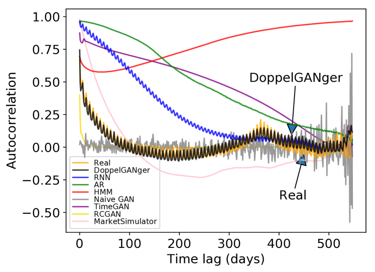
Figure 1. Autocorrelation of daily page views for Wikipedia Web Traffic dataset.

Machine-learned models:  These are general parametric models, where the parameters can be learned (trained) from data. Examples include autoregressive models, Markov models, and recurrent neural networks (RNNs). In theory, these generic statistical models have the potential to generalize across datasets. However, they are not general in terms of use cases, because they do not jointly model metadata and time series. For example, in a network measurement dataset, modeling only the packet loss rate is good for understanding its patterns. But if we want to learn which IP prefix has network issues, jointly modeling the metadata (IP address) and the time series (sequence of packet loss rate) is important. Additionally, these general-purpose models have bad fidelity, failing to capture long-term temporal correlations. For instance, all these models fail to capture weekly and/or annual patterns in the Wikipedia Web Traffic dataset (Figure 1). Our point is not to highlight the importance of learning autocorrelations, but to show that learning temporal data distributions (without overfitting to a single statistic, e.g. autocorrelation) is hard. Note that DG is able to learn weekly and annual correlations without special tuning.

3. Overview

As we saw, the above classes of techniques do not achieve good fidelity and generality across datasets and use cases. Our overarching goal is thus to develop a general framework that can achieve high fidelity with minimal expertise.

3.1. Problem formulation

We abstract the scope of our datasets as follows: A dataset $\mathcal{D}=\big{\{}O^{1},O^{2},\allowbreak...,O^{n}\big{\}}$ is defined as a set of samples $O^{i}$ (e.g., the clients). Each sample $O^{i}=(A^{i},R^{i})$ contains $m$ metadata $A^{i}=[A^{i}_{1},A^{i}_{2},...,A^{i}_{m}]$. For example, metadata $A^{i}_{1}$ could represent client $i$’s physical location, and $A^{i}_{2}$ the client’s ISP. Note that we can support datasets in which multiple samples have the same set of metadata. The second component of each sample is a time series of records $R^{i}=[R^{i}_{1},R^{i}_{2},...,R^{i}_{T^{i}}]$, where $R^{i}_{j}$ means $j$-th measurement of $i$-th client. Different samples may contain a different number of measurements. The number of records for sample $O^{i}$ is given by $T^{i}$. Each record $R^{i}_{j}=(t^{i}_{j},f^{i}_{j})$ contains a timestamp $t^{i}_{j}$, and $K$ measurements $f^{i}_{j}=[f^{i}_{j,1},f^{i}_{j,2},...,f^{i}_{j,K}]$. For example, $t^{i}_{j}$ represents the time when the measurement $f^{i}_{j}$ is taken, and $f^{i}_{j,1}$, $f^{i}_{j,2}$ represent the ping loss rate and traffic byte counter at this timestamp respectively. Note that the timestamps are sorted, i.e. $t^{i}_{j}<t^{i}_{j+1}\leavevmode\nobreak\ \forall 1\leq j<T^{i}$.

This abstraction fits many classes of data that appear in networking applications. For example, it is able to express web traffic and cluster trace datasets (§5). Our problem is to take any such dataset as input and learn a model that can generate a new dataset $\mathcal{D}^{\prime}$ as output. $\mathcal{D}^{\prime}$ should exhibit fidelity, and the methodology should be general enough to handle datasets in our abstraction.

3.2. GANs: background and promise

GANs are a data-driven generative modeling technique (Goodfellow et al., 2014) that take as input training data samples and output a model that can produce new samples from the same distribution as the original data. More precisely, if we have a dataset of $n$ samples $O_{1},\ldots,O_{n}$, where $O_{i}\in\mathbb{R}^{p}$, and each sample is drawn i.i.d. from some distribution $O_{i}\sim P_{O}$. The goal of GANs is to use these samples to learn a model that can draw samples from distribution $P_{O}$ (Goodfellow et al., 2014).

GANs use an adversarial training workflow consisting of a generator $G$ and a discriminator $D$ (Figure 2). In practice, both are instantiated with neural networks. In the canonical GAN design (Goodfellow et al., 2014), the generator maps a noise vector $z\in\mathbb{R}^{d}$ to a sample $O\in\mathbb{R}^{p}$, where $p\gg d$. $z$ is drawn from some pre-specified distribution $P_{z}$, usually a Gaussian or a uniform. Simultaneously, we train the discriminator $D:\mathbb{R}^{p}\to[0,1]$, which takes samples as input (either real of fake), and classifies each sample as real (1) or fake (0). Errors in this classification task are used to train the parameters of both the generator and discriminator through backpropagation. The loss function for GANs is: $\min_{G}\max_{D}\mathbb{E}_{x\sim p_{x}}[\log D(x)]+\mathbb{E}_{z\sim p_{z}}[\log(1-D(G(z)))].$ The generator and discriminator are trained alternately, or adversarially. Unlike prior generative modeling approaches which likelihood maximization of parametric models (e.g., §2.2), GANs make fewer assumptions about the data structure.

Compared with related work in §2.2, GANs offer three key benefits. First, similar to the machine learning models, GANs can be general across datasets. The discriminator is an universal agent for judging the fidelity of generated samples. Thus, the discriminator only needs raw samples and it does not need any other information about the system producing the samples. Second, GANs can be used to generate measurements and metadata (§3.3.2). Thus, GANs have the potential to support a wide range of use cases involving measurements, metadata, and cross-correlations between them. Finally, GANs have been used in other domains for generating realistic high-fidelity datasets for complex tasks such as images (Karras et al., 2017), text (Fedus et al., 2018; Yu et al., 2017), and music (Mogren, 2016; Dong et al., 2018).

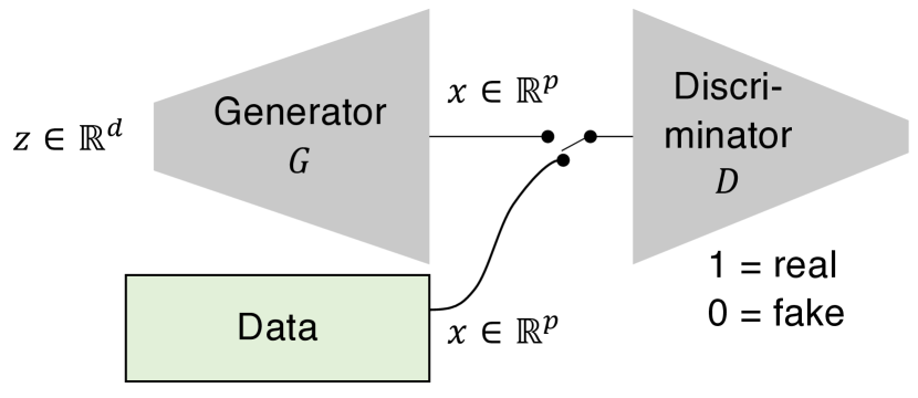
Figure 2. Original GAN architecture from (Goodfellow et al., 2014).

3.3. Using GANs to generate time series

3.3.1. Prior Work.

Using GANs to generate time series is a popular idea (Fedus et al., 2018; Yu et al., 2017; Mogren, 2016; Dong et al., 2018; Esteban et al., 2017; Zec et al., 2019; Yoon et al., 2019; Fu and Xu, 2007). Among the domain-agnostic designs, the generator usually takes prior measurements (generated or real) and noise as inputs and outputs one measurement at a time (Fu and Xu, 2007; Esteban et al., 2017; Zec et al., 2019; Yoon et al., 2019; Yu et al., 2017). These works typically change two aspects of the GAN: the architecture (Fu and Xu, 2007; Esteban et al., 2017; Zec et al., 2019), the training (Yu et al., 2017), or both (Yoon et al., 2019; Buehler et al., 2020). The two most relevant papers to ours are RCGAN (Esteban et al., 2017) and TimeGAN (Yoon et al., 2019). RCGAN is the most similar design to ours; like DG, it uses recurrent neural networks (RNNs) to generate time series and can condition the generation on metadata. However, RCGAN does not itself generate metadata and has little to no evaluation of the correlations across time series and between metadata and measurements. We found its fidelity on our datasets to be poor; we instead use a different discriminator architecture, loss function, and measurement generation pipeline (§4). TimeGAN is the current state-of-the-art, outperforming RCGAN (Yoon et al., 2019). Like RCGAN, it uses RNNs for both the generator and discriminator. Unlike RCGAN, it trains an additional neural network that maps time series to vector embeddings, and the generator outputs sequences of embeddings rather than samples. Learning to generate transformed or embedded time series is common, both in approaches that rely on GANs (Yoon et al., 2019; Marti, 2020) and those that rely on a different class of generative models called variational autoencoders (VAE) (Buehler et al., 2020). Our experiments suggest that this approach models long time series poorly (§5).

3.3.2. Challenges.

Next, we highlight key challenges that arise in using GANs for our use cases. While these challenges specifically stem from our attempts in using GANs in networking- and systems–inspired use cases, some of these challenges broadly apply to other use cases as well.

Fidelity challenges:  The first challenge relates to long-term temporal correlations. As we see in Figure 1, the canonical GAN does poorly in capturing temporal correlations trained on the Wikipedia Web Traffic (WWT) dataset. Concurrent and prior work on using GANs for other time series data has also observed this (Fedus et al., 2018; Yu et al., 2017; Esteban et al., 2017; Yoon et al., 2019). One approach to address this is segmenting long datasets into chunks; e.g., TimeGAN (Yoon et al., 2019) chunks datasets into smaller time series each of 24 epochs, and only evaluates the model on producing new time series of this length (Yoon, [n. d.]). This is not viable in our domain, as relevant properties of networking/systems data often occur over longer time scales (e.g., network measurements) (see Figure 1). Second, mode collapse is a well-known problem in GANs where they generate only a few modes of the underlying distribution (Srivastava et al., 2017; Lin et al., 2018; Arjovsky et al., 2017; Gulrajani et al., 2017). It is particularly exacerbated in our time series use cases because of the high variability in the range of measurement values. Finally, we need to capture complex relations between measurements and metadata (e.g., packet loss rate and ISP), and across different measurements (e.g., packet loss rate and byte counts). As such, state-of-the-art approaches either do not co-generate attributes with time series data or their accuracy for such tasks is unknown (Esteban et al., 2017; Zec et al., 2019; Yoon et al., 2019), and directly generating joint metadata with measurements samples does not converge (§5). Further, generating independent time series for each measurementdimension will break their correlations.

Privacy challenges:  In addition to the above fidelity challenges, we also observe key challenges with respect to privacy, and reasoning about the privacy-fidelity tradeoffs of using GANs. A meta question, not unique to our work, is finding the right definition of privacy for each use case. Some commonly used definitions in the community are notions of differential privacy (i.e., how much does any single data point contribute to a model) (Dwork, 2008) and membership inference (i.e., was a specific sample in the datasets) (Shokri et al., 2017). However, these definitions can hurt fidelity (Sankar et al., 2013; Bagdasaryan et al., 2019) without defending against relevant attacks (Fredrikson et al., 2014; Hitaj et al., 2017). In our networking/systems use cases, we may also want to even hide specific features and avoid releasinng aggregate statistical characteristics of proprietary data (e.g., number of users, server load, meantime to failure). Natural questions arise: First, can GANs support these flexible notions of privacy in practice, and if so under what configurations? Second, there are emerging proposals to extend GAN training (e.g., (Xie et al., 2018; Xu et al., 2019; Frigerio et al., 2019)) to offer some privacy guarantees. Are their privacy-fidelity tradeoffs sufficient to be practical for networking datasets?

4. DoppelGANger Design

In this section, we describe how we tackle fidelity shortcomings of time series GANs. Privacy is discussed in Section 6. Recall that existing approaches have issues in capturing temporal effects and relations between metadata and measurements. In what follows, we present our solution starting from the canonical GAN strawman and extend it to address these challenges. Finally, we summarize the design and guidelines for users to use our workflow.

4.1. Capturing long-term effects

Recall that the canonical GAN generator architecture is a fully-connected multi-layer perceptron (MLP), which we use in our strawman solution (§3.3.2). As we saw, this architecture fails to capture long-term correlations (e.g., annual correlations in page views).

RNN primer and limitations:  Similar to prior efforts, we posit that the main reason is that MLPs are not well suited for time series. A better choice is to use recurrent neural networks (RNNs), which are designed to model time series and have been widely used in the GAN literature to generate time series (Mogren, 2016; Esteban et al., 2017; Yu et al., 2017; Zec et al., 2019; Yoon et al., 2019). Specifically, we use a variant of RNN called long short-term memory (LSTM) (Hochreiter and Schmidhuber, 1997).

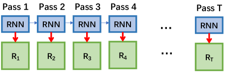
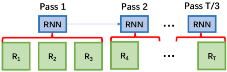
Figure 3. (a) The usual way of generating time series. (b) Batch generation with $S=3$. The RNN is a single neural network, even though many units are illustrated. This unrolled representation conveys that the RNN is being used many times to generate samples.

At a high level, RNNs work as follows (Figure 3 (a)). Instead of generating the entire time series at once, RNNs generate one record $R_{j}^{i}$ at a time (e.g., page views on the $j$th day), and then run $T^{i}$ (e.g., the number of days) passes to generate the entire time series. The key difference in a RNN from traditional neural units is that RNNs have an internal state that implicitly encodes all past states of the signal. Thus, when generating $R_{j}^{i}$, the RNN unit can incorporate the patterns in $R_{1}^{i},...,R_{j-1}^{i}$ (e.g., all page views before the $j$-th day). Note that RNNs can learn correlations across the dimensions of a time series, and produce multi-dimensional outputs.

However, we empirically find that RNN generators still struggle to capture temporal correlations when the length exceeds a few hundred epochs. The reason is that for long time series, RNNs take too many passes to generate the entire sample; the more passes taken, the more temporal correlation RNNs tend to forget. Prior work copes with this problem in three ways. The first is to generate only short sequences (Mogren, 2016; Yu et al., 2017; Yoon et al., 2019); long datasets are evaluated on chunks of tens of samples (Yoon et al., 2019; Yoon, [n. d.]). The second approach is to train on small datasets, where rudimentary designs may be able to effectively memorize long term effects (e.g. unpublished work (De Meer, Fernando, 2019) generates time series of length 1,000, from a dataset of about $100$ time series). This approach leads to memorization (Arora and Zhang, 2017), which defeats the purpose of training a model. A third approach assumes an auxiliary raw data time series as an additional input during the generation phase to help generate long time series (Zec et al., 2019). This again defeats the purpose of synthetic data generation.

Our approach:  To reduce the number of RNN passes, we propose to use a simple yet effective idea called batch generation. At each pass of the RNN, instead of generating one record (e.g., page views of one day), it generates $S$ records (e.g., page views of $S$ consecutive days), where $S$ is a tunable parameter (Figure 3 (b)). This effectively reduces the total number of RNN passes by a factor of $S$. As $S$ gets larger, the difficulty of synthesizing a batch of records at a single RNN pass also increases. This induces a natural trade-off between the number of RNN passes and the single pass difficulty. For example, Figure 4 shows the mean square error between the autocorrelation of our generated signals and real data on the WWT dataset. Even a small (but larger than 1) $S$ gives substantial improvements in signal quality. In practice, we find that $S=5$ works well for many datasets and a simple autotuning of this hyperparameter similar to this experiment can be used in practice (§4.4).

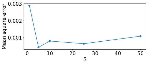
Figure 4. Error vs. batch parameter.

The above workflow of using RNNs with batch generation ignores the timestamps from generation. In practice, for some datasets, the timestamps may be important in addition to timeseries samples; e.g., if derived features such as inter-arrival times of requests may be important for downstream systems and networking tasks. To this end, we support two simple alternatives. First, if the raw timestamps are not important, we can assume that they are equally spaced and are the same for all samples (e.g., when the dataset is daily page views of websites). Second, if the derived temporal properties are critical, we can simply use the initial timestamp of each sample as an additional metadata (i.e., start time of the sample) and the inter-arrival times between consecutive records as an additional measurement.

4.2. Tackling mode collapse

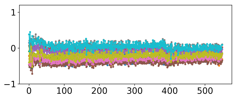
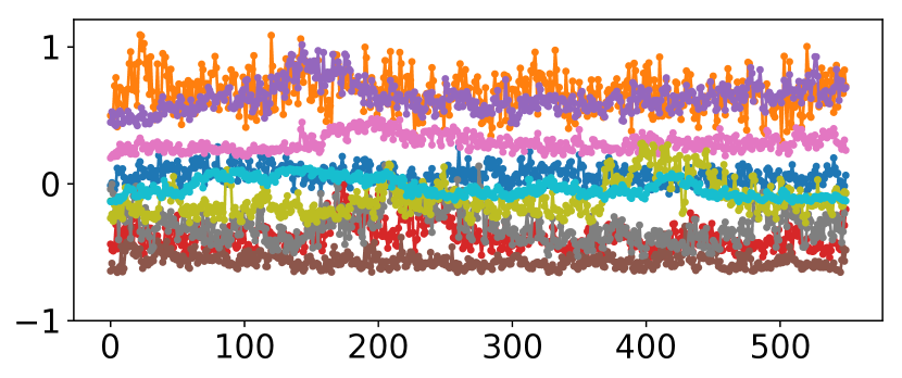
Figure 5. Without auto-normalization, generated samples show telltale signs of mode collapse as they have similar shapes and amplitudes.

Mode collapse is a well-known problem (Goodfellow, 2016), where the GAN outputs homogeneous samples despite being trained on a diverse dataset. For example, suppose we train on web traffic data that includes three distinct kinds of signals, corresponding to different classes of users. A mode-collapsed GAN might learn to generate only one of those traffic types.

For instance, fig. 5 (top) plots synthetic time series from a GAN trained on the WWT dataset, normalized and shifted to $[-1,1]$. The generated samples are heavily mode-collapsed, exhibiting similar amplitudes, offsets, and shapes.

Existing work and limitations:  Alleviating mode collapse is an active research topic in the GAN community (e.g., (Srivastava et al., 2017; Lin et al., 2018; Arjovsky et al., 2017; Gulrajani et al., 2017)). We experimented with a number of state-of-the-art techniques for mitigating mode collapse (Lin et al., 2018; Gulrajani et al., 2017). However, these did not resolve the problem on our datasets.

Our approach:  Our intuition is that unlike images or medical data, where value ranges tend to be similar across samples, networking datasets exhibit much higher range variability. Datasets with a large range (across samples) appear to worsen mode collapse because they have a more diverse set of modes, making them harder to learn. For example, in the WWT dataset, some web pages consistently have $>$2000 page views per day, whereas others always have $<$10.

Rather than using a general solution for mode collapse, we build on this insight to develop a custom auto-normalization heuristic. Recall that each time series of measurements $f^{i}$ (e.g., network traffic volume measurement of a client) is also assigned some metadata $A^{i}$ (e.g., the connection technology of the client, cable/fiber). Suppose our dataset has two time series with different offsets: $f^{1}(t)=\sin(t)$ and $f^{2}(t)=\sin(t)+100$ and no metadata, so $A^{1}=A^{2}=()$. We have $\min(f^{1})=-1$, $\max(f^{1})=2$, $\min(f^{2})=99$, $\max(f^{2})=101$. A standard normalization approach (e.g. as in (Yoon, [n. d.])) would be to simply normalize this data by the global min and max, store them as global constants, and train on the normalized data. However, this is just scaling and shifting by a constant; from the GAN’s perspective, the learning problem is the same, so mode collapse still occurs.

Instead, we normalize each time series signal individually, and store the min/max as “fake” metadata. Rather than training on the original $(f^{i},A^{i})$ pairs, we train on $\tilde{f}^{1}(t)=\sin(t)$, $\tilde{A}^{1}=(-1,1)$, $\tilde{f}^{2}(t)=\sin(t)$, $\tilde{A}^{2}=(99,101)$. Hence, the GAN learns to generate these two fake metadata defining the max/min for each time series individually, which are then used to rescale measurements to a realistic range.

Note that this approach differs from typical feature normalization in two ways: (1) it normalizes each sample individually, rather than normalizing over the entire dataset, and (2) it treats the maximum and minimum value of each time series as a random variable to be learned (and generated). In this way, all time series have the same range during generation, which alleviates the mode collapse problem. Figure 5 (bottom) shows that by training DG with auto-normalization on the WWT data, we generate samples with a broad range of amplitudes, offsets, and shapes.

4.3. Capturing attribute relationships

So far, we have only discussed how to generate time series. However, metadata can strongly influence the characteristics of measurements. For example, fiber users tend to use more traffic than cable users. Hence, we need a mechanism to model the joint distribution between measurements and metadata. As discussed in §3.3.2, naively generating concatenated metadata $A^{i}$ and measurements $R^{i}$ does not learn the correlations between them well. We hypothesize that this is because jointly generating metadata and measurements using a single generator is too difficult.

Existing work and limitations:  A few papers have tackled this problem, mostly in the context of generating multidimensional data. The dominant approach in the literature is to train a variant of GANs called conditional GANs (CGANs), which learn to produce data conditioned on a user-provided input label. For example, prior works (Esteban et al., 2017; Fu et al., 2019; Zec et al., 2019) learn a conditional model in which the user inputs the desired metadata, and the architecture generates measurements conditioned on the attributes; generating the attributes as well is a simple extension (Esteban et al., 2017). TimeGAN claims to co-generate metadata and measurements, but it does not evaluate on any datasets that include metadata in the paper, nor does the released code handle metadata (Yoon et al., 2019; Yoon, [n. d.]).

Our approach:  We start by decoupling this problem into two sub-tasks: generating metadata and generating measurements conditioned on metadata: $P(A^{i},R^{i})=P(A^{i})\cdot P(R^{i}|A^{i})$, each using a dedicated generator; this is is conceptually similar to prior approaches (Esteban et al., 2017; Zec et al., 2019). More specifically, we use a standard multi-layer perceptron (MLP) network for generating the metadata. This is a good choice, as MLPs are good at modeling (even high-dimensional) non-time-series data. For measurement generation, we use the RNN-based architecture from §4.1. To preserve the hidden relationships between the metadata and the measurements, the generated metadata $A^{i}$ is added as an input to the RNN at every step.

Recall from section 4.2 that we treat the max and min of each time series as metadata to alleviate mode collapse. Using this conditional framework, we divide the generation of max/min metadata into three steps: (1) generate “real” metadata using the MLP generator (§4.3); (2) with the generated metadata as inputs, generate the two “fake” (max/min) metadata using another MLP; (3) with the generated real and fake metadata as inputs, generate measurements using the architecture in §4.1 (see Figure 7).

Unfortunately, a decoupled architecture alone does not solve the problem. Empirically, we find that when the average length of measurements is long (e.g., in the WWT dataset, each sample consists of 550 consecutive daily page views), the fidelity of generated data—especially the metadata—is poor. To understand why, recall that a GAN discriminator judges the fidelity of generated samples and provides feedback for the generator to improve. When the total dimension of samples (measurements + metadata) is large, judging sample fidelity is hard.

Motivated by this, we introduce an auxiliary discriminator which discriminates only on metadata. The losses from two discriminators are combined by a weighting parameter $\alpha$: $\min_{G}\max_{D_{1},D_{2}}\mathcal{L}_{1}(G,D_{1})+\alpha\mathcal{L}_{2}(G,D_{2})$ where $\mathcal{L}_{i}$, $i\in\{1,2\}$ is the Wasserstein loss of the original and the auxiliary discriminator respectively. The generator effectively learns from this auxiliary discriminator to generate high-fidelity metadata. Further, with the help of the original discriminator, the generator can learn to generate measurements well.

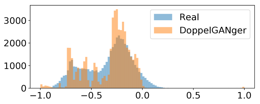
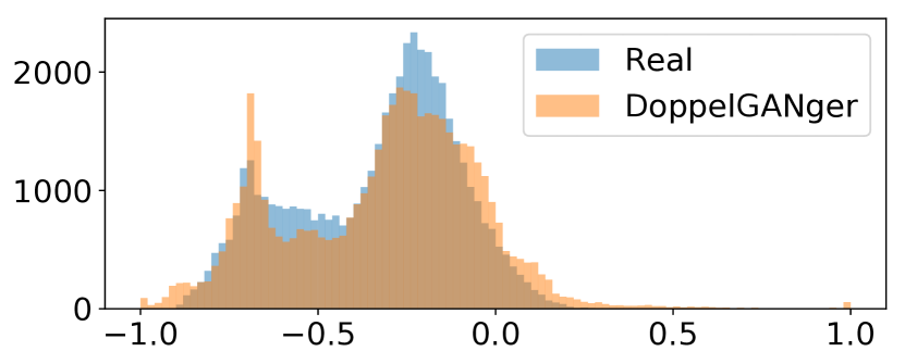
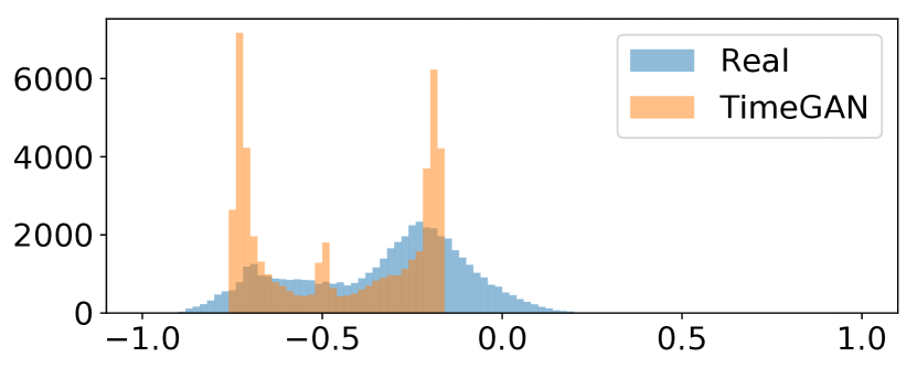
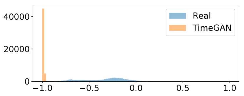
Figure 6. Distribution of (max+min)/2 of (a) DG without and (b) DG with the auxiliary discriminator, (c) TimeGAN, and (d) RCGAN (WWT data).

Empirically, we find that this architecture improves the data fidelity significantly. Figure 6 shows a histogram of the (max$+$min)/2 metadata distribution from DG on the WWT dataset. That is, for each time series, we extract the maximum and minimum value, and compute their average; then we compute a histogram of these averages over many time series. This distribution implicitly reflects how well DG reproduces the range of time series values in the dataset. We observe that adding the auxiliary discriminator significantly improves the fidelity of the generated distribution, particularly in the tails of the true distribution.

4.4. Putting it all together

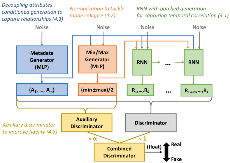
Figure 7. Architecture of DG highlighting key ideas and extensions to canonical GAN approaches.

The overall DG architecture is in Figure 7, highlighting the key differences from canonical approaches. First, to capture the correlations between metadata and measurements, we use a decoupled generation of metadata and measurements using an auxiliary discriminator, and conditioning the measurements based on the metadata generated. Second, to address the mode collapse problem for the measurements, we add the fake metadata capturing the min/max values for each generated sample. Third, we use a batched RNN generator to capture the temporal correlations and synthesize long time series that are representative.

The training phase requires two primary inputs: the data schema (i.e., metadata/measurement dimensions, indicating whether they are categorical or numeric) and the training data. The only minimal tuning that data holders sharing a dataset using DG need to be involved in is selecting the measurement batch size $S$ (§4.1) controls the number of measurements generated at each RNN pass. Empirically, setting $S$ so that $T/S$ (the number of steps RNN needs to take) is around 50 gives good results, whereas prior time series GANs use $S=1$ (Esteban et al., 2017; Beaulieu-Jones et al., 2017; Yoon et al., 2019; Zec et al., 2019). Optionally, data holders can specify sensitive metadata, whose distribution can be masked or request additional privacy settings to be used (§6). We envision data holders sharing the generative model with the data users. Users can then flexibly use this model and also optionally specify different metadata distribution (e.g., for amplifying rare events) if needed. That said, our workflow also accommodates a more restrictive mode of sharing, where the holder uses DG to generate synthetic data internally and then releases the generated data without sharing the model.

The code and a detailed documentation (on data format, hyper-parameter setting, model training, data generation, etc.) are available at https://github.com/fjxmlzn/DoppelGANger.

5. Fidelity Evaluation

We evaluate the fidelity of DG on three datasets, whose properties are summarized in Table 1.

5.1. Setup

5.1.1. Datasets

These datasets are chosen to exhibit different combinations of challenges: (1) correlations within time series and metadata, (2) multi-dimensional measurements, and/or (3) variable measurement lengths.

Dataset	Correlated in time & metadata	Multi-dimensional measurements	Variable-length signals
WWT (Google, 2018)	x
MBA (Commission, 2018)	x	x
GCUT (Reiss et al., 2011)	x	x	x

Table 1. Challenging properties of studied datasets.

Wikipedia Web Traffic (WWT):  This dataset tracks the number of daily views of Wikipedia articles, starting from July 1st, 2015 to December 31st, 2016 (Google, 2018). In our language, each sample is a page view counter for one Wikipedia page, with three metadata: Wikipedia domain, type of access (e.g., mobile, desktop), and type of agent (e.g., spider). Each sample has one measurement: the number of daily page views.

Measuring Broadband America (MBA):  This dataset was collected by United States Federal Communications Commission (FCC) (Commission, 2018) and consists of several measurements such as round-trip times and packet loss rates from several clients in geographically diverse homes to different servers using different protocols (e.g. DNS, HTTP, PING). Each sample consists of measurements from one device. Each sample has three metadata: Internet connection technology, ISP, and US state. A record contains UDP ping loss rate (min.  across measured servers) and total traffic (bytes sent and received), reflecting client’s aggregate Internet usage.

Google Cluster Usage Traces (GCUT):  This dataset (Reiss et al., 2011) contains usage traces of a Google Cluster of 12.5k machines over 29 days in May 2011. We use the logs containing measurements of task resource usage, and the exit code of each task. Once the task starts, the system measures its resource usage (e.g. CPU usage, memory usage) per second, and logs aggregated statistics every 5 minutes (e.g., mean, maximum). Those resource usage values are the measurements. When the task ends, its end event type (e.g. FAIL, FINISH, KILL) is also logged. Each task has one end event type, which we treat as an metadata.

More details of the datasets (e.g. dataset schema) are attached in Appendix A.

5.1.2. Baselines

We only compare DG to the baselines in §2.2 that are general—the machine-learned models. (In the interest of reproducibility, we provide complete configuration details for these models in Appendix B.)

Hidden Markov models (HMM) (§2.2):  While HMMs have been used for generating time series data, there is no natural way to jointly generate metadata and time series in HMMs. Hence, we infer a separate multinomial distribution for the metadata. During generation, metadata are randomly drawn from the multinomial distribution on training data, independently of the time series.

Nonlinear auto-regressive (AR) (§2.2):  Traditional AR models can only learn to generate measurements. In order to jointly learn to generate metadata and measurements, we design the following more advanced version of AR: we learn a function $f$ such that $R_{t}=f(A,R_{t-1},R_{t-2},...,R_{t-p})$. To boost the accuracy of this baseline, we use a multi-layer perceptron version of $f$. During generation, $A$ is randomly drawn from the multinomial distribution on training data, and the first record $R_{1}$ is drawn a Gaussian distribution learned from training data.

Recurrent neural networks (RNN) (§2.2):  In this model, we train an RNN via teacher forcing (Williams and Zipser, 1989) by feeding in the true time series at every time step and predicting the value of the time series at the next time step. Once trained, the RNN can be used to generate the time series by using its predicted output as the input for the next time step. A traditional RNN can only learn to generate measurements. We design an extended RNN takes metadata $A$ as an additional input. During generation, $A$ is randomly drawn from the multinomial distribution on training data, and the first record $R_{1}$ is drawn a Gaussian distribution learned from training data.

Naive GAN (§3.3.2):  We include the naive GAN architecture (MLP generator and discriminator) in all our evaluations.

TimeGAN (Yoon et al., 2019):  Note that the state-of-the-art TimeGAN (Yoon, [n. d.]) does not jointly generate metadata and high-dimensional time series of different lengths, so several of our evaluations cannot be run on TimeGAN. However, we modified the TimeGAN implementation directly (Yoon, [n. d.]) to run on the WWT dataset (without metadata) and compared against it.

RCGAN (Esteban et al., 2017):  RCGAN does not generate metadata, and only deals with time series of the same length, so again, several of our evaluations cannot be run on RCGAN. To make a comparison, we used the version without conditioning (called RGAN (Esteban et al., 2017)) from the official implementation (Esteban et al., [n. d.]) and evaluate it on the WWT dataset (without metadata).

Market Simulator (Buehler et al., 2020):  We also compare against a VAE-based approach (Buehler et al., 2020) designed to generate synthetic financial market data, since its code is publicly available.

5.1.3. Metrics

Evaluating GAN fidelity is notoriously difficult (Lucic et al., 2018; Xu et al., 2018); the most widely-accepted metrics are designed for labelled image data (Salimans et al., 2016; Heusel et al., 2017) and cannot be applied to our datasets. Moreover, numeric metrics do not always capture the qualitative problems of generative models. We therefore evaluate DG with a combination of qualitative and quantitative microbenchmarks and downstream tasks that are tailored to each of our datasets. Our microbenchmarks evaluate how closely a statistic of the generated data matches the real data. E.g., the statistics could be attribute distributions or autocorrelations, and the similarity can be evaluated qualitatively or by computing an appropriate distance metric (e.g., mean square error, Jensen-Shannon divergence). Our downstream tasks use the synthetic data to reason about the real data, e.g., attribute prediction or algorithm comparison. In line with the recommendations of (Lucic et al., 2018), these tasks can be evaluated with quantitative, task-specific metrics like prediction accuracy. Each metric is explained in more detail inline.

5.2. Results

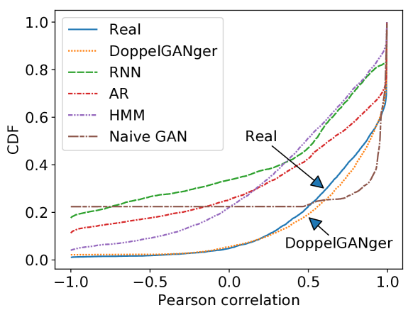
Figure 8. CDF of Pearson correlation between CPU rate and assigned memory usage from GCUT.

Structural characterization:  In line with prior recommendations (Melamed and Hill, 1993), we explore how DG captures structural data properties like temporal correlations, metadata distributions, and metadata-measurement joint distributions.

Temporal correlations: To show how DG captures temporal correlations, Figure 1 shows the average autocorrelation for the WWT dataset for real and synthetic datasets (discussed in §2.2). As mentioned before, the real data has a short-term weekly correlation and a long-term annual correlation. DG captures both, as evidenced by the periodic weekly spikes and the local peak at roughly the 1-year mark, unlike our baseline approaches. It also exhibits a 91.2% lower mean square error from the true data autocorrelation than the closest baseline (RCGAN).

The fact that DG captures these correlations is surprising, particularly since we are using an RNN generator. Typically, RNNs are able to reliably generate time series of length around 20, while the length of WWT measurements is 550. We believe this is due to a combination of adversarial training (not typically used for RNNs) and our batch generation. Empirically, eliminating either feature hurts the learned autocorrelation. TimeGAN and RCGAN, for instance, use RNNs and adversarial training but does not batch generation, though its performance may be due to other architectural differences (Yoon et al., 2019; Esteban et al., 2017). E.g., WWT is an order of magnitude longer than the time series it evaluates on (Yoon, [n. d.]; Esteban et al., [n. d.]).

Another aspect of learning temporal correlations is generating time series of the right length. Figure 9 shows the duration of tasks in the GCUT dataset for real and synthetic datasets generated by DG and RNN. Note that TimeGAN generates time series of different lengths by first generating time series of a maximum length and then truncating according to the empirical length distribution from the training data (Yoon, [n. d.]). Hence we do not compare against TimeGAN because the comparison is not meaningful; it perfectly reproduces the empirical length distribution, but not because the generator is learning to reproduce time series lengths.

DG’s length distribution fits the real data well, capturing the bimodal pattern in real data, whereas RNN fails. Other baselines are even worse at capturing the length distribution (Appendix C). We observe this regularly; while DG captures multiple data modes, our baselines tend to capture one at best. This may be due to the naive randomness in the other baselines. RNNs and AR models incorporate too little randomness, causing them to learn simplified duration distributions; HMMs instead are too random: they maintain too little state to generate meaningful results.

Figure 9. Histogram of task duration for the Google Cluster Usage Traces. RNN-generated data misses the second mode, but DoppelGANger captures it.

Cross-measurement correlations: To evaluate correlations between the dimensions of our measurements, we computed the Pearson correlation between the CPU and memory measurements of generated samples from the GCUT dataset. Figure 8 shows the CDF of these correlation coefficients for different time series. We observe that DG much more closely mirrors the true auto-correlation coefficient distribution than any of our baselines.

Measurement distributions: As discussed in §4.3 and Figure 7, DG captures the distribution of (max+min)/2 of page views in WWT dataset. As a comparison, TimeGAN and RCGAN have much worse fidelity. TimeGAN captures the two modes in the distribution, but fails to capture the tails. RCGAN does not learn the distribution at all. In fact, we find that RCGAN has severe mode collapse in this dataset: all the generated values are close to -1. Some possible reasons might be: (1) The maximum sequence length experimented in RCGAN is 30 (Esteban et al., [n. d.]), whereas the sequence length in WWT is 550, which is much more difficult; (2) RCGAN used different numbers of generator and discriminator updates per step in different datasets (Esteban et al., [n. d.]). We directly take the hyper-parameters from the longest sequence length experiment in RCGAN’s code (Esteban et al., [n. d.]), but other fine-tuned hyper-parameters might give better results. Note that unlike RCGAN, DG is able to achieve good results in our experiments without tuning the numbers of generator and discriminator updates.

Metadata distributions: Learning correct metadata distributions is necessary for learning measurement-metadata correlations. As mentioned in §5.1.2, for our HMM, AR, and RNN baselines, metadata are randomly drawn from the multinomial distribution on training data because there is no clear way to jointly generate metadata and measurements. Hence, they trivially learn a perfect metadata distribution. Figure 10 shows that DG is also able to mimic the real distribution of end event type distribution in GCUT dataset, while naive GANs miss a category entirely; this appears to be due to mode collapse, which we mitigate with our second discriminator. Results on other datasets are in Appendix C.

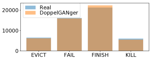
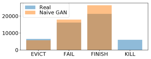
Figure 10. Histograms of end event types from GCUT.

Measurement-metadata correlations: Although our HMM, AR, and RNN baselines learn perfect metadata distributions, it is substantially more challenging (and important) to learn the joint metadata-measurement distribution. To illustrate this, we compute the CDF of total bandwidth for DSL and cable users in MBA dataset. Table 2 shows the Wasserstein-1 distance between the generated CDFs and the ground truth, showing that DG is closest to the real distribution. CDF figures are attached in Appendix C.

	DoppelGANger	AR	RNN	HMM	Naive GAN
DSL	0.68	1.34	2.33	3.46	1.14
Cable	0.74	6.57	2.46	7.98	0.87

Table 2. Wasserstein-1 distance of total bandwidth distribution of DSL and cable users. Lower is better.

DG does not overfit: In the context of GANs, overfitting is equivalent to memorizing the training data, which is a common concern with GANs (Arora and Zhang, 2017; Odena et al., 2017). To evaluate this, we ran an experiment inspired by the methodology of (Arora and Zhang, 2017): for a given generated DG sample, we find its nearest samples in the training data. We observe significant differences (both in square error and qualitatively) between the generated samples and the nearest neighbors on all datasets, suggesting that DG is not memorizing. Examples can be found in Appendix C.

Resource costs: DG has two main costs: training data and training time/computation. In Figure 11, we plot the mean square error (MSE) between the generated samples’ autocorrelations and the real data’s autocorrelations on the WWT dataset as a function of training set size. MSE is sensitive to training set size—it decreases by 60% as the training data grows by 2 orders of magnitude. However, Table 3 shows that DG trained on 500 data points (the size that gives DG the worst performance) still outperforms all baselines trained on 50,000 samples in autocorrelation MSE. Figure 11 also illustrates variability between models; due to GAN training instability, different GAN models with the same hyperaparameters can have different fidelity metrics. Such training failures can typically be detected early in the training proccess.

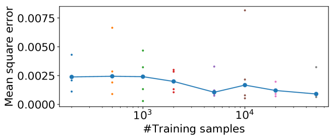
Figure 11. Mean square error of autocorrelation of the daily page views v.s. number of training samples for WWT dataset. For each training set size, 5 independent runs are executed and their MSE are plotted in the figure. The line connects the median MSE of the 5 independent runs.

Method	MSE
RNN	0.1222
AR	0.2777
HMM	0.6030
Naive GAN	0.0190
TimeGAN	0.2384
RCGAN	0.0103
MarketSimulator	0.0324
DoppelGANger	0.0009
DoppelGANger (500 training samples)	0.0024

Table 3. Mean square error (MSE) of autocorrelation of the daily page views for WWT dataset (i.e. quantitative presentation of Figure 1). Each model is trained with multiple independent runs, and the median MSE among the runs is presented. Except the last row, all models are trained with 50000 training samples.

With regards to training time, Table 4 lists the training time for DG and other baselines. All models were trained on a single NVIDIA Tesla V100 GPU with 16GB GPU memory and an Intel Xeon Gold 6148 CPU with 24GB RAM. These implementations have not been optimized for performance at all, but we find that on the WWT dataset, DG requires 17 hours on average to train, which is $3.4\times$ slower than the fastest benchmark (Naive GAN) and $15.2\times$ faster than the slowest benchmark (TimeGAN).

Method	Average training time (hrs)
Naive GAN	5
Market Simulator	6
HMM	8
RNN	22
RCGAN	29
AR	93
TimeGAN	258
DoppelGANger	17

Table 4. Average training time (hours) of synthetic data models on the WWT dataset. All models are trained with 50000 training samples.

Predictive modeling:  Given time series measurements, users may want to predict whether an event $E$ occurs in the future, or even forecast the time series itself. For example, in GCUT dataset, we could predict whether a particular job will complete successfully. In this use case, we want to show that models trained on generated data generalize to real data.

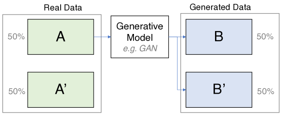
Figure 12. Predictive modeling setup: Using training data $A$, we generate samples $B\cup B^{\prime}$. Subsequent experiments train downstream tasks on $A$ or $B$, our training sets, and then test on $A^{\prime}$ or $B^{\prime}$.

We first partition our dataset, as shown in Figure 12. We split real data into two sets of equal size: a training set A and a test set A’. We then train a generative model (e.g., DG or a baseline) on training set A. We generate datasets B and B’ for training and testing. Finally, we evaluate event prediction algorithms by training a predictor on A and/or B, and testing on A’ and/or B’. This allows us to compare the generalization abilities of the prediction algorithms both within a class of data (real/generated), and generalization across classes (train on generated, test on real) (Esteban et al., 2017).

We first predict the task end event type on GCUT data (e.g., EVICT, KILL) from time series observations. Such a predictor may be useful for cluster resource allocators. This prediction task reflects the correlation between the time series and underlying metadata (namely, end event type). For the predictor, we trained various algorithms to demonstrate the generality of our results: multilayer perceptron (MLP), Naive Bayes, logistic regression, decision trees, and a linear SVM. Figure 13 shows the test accuracy of each predictor when trained on generated data and tested on real. Real data expectedly has the highest test accuracy. However, we find that DG performs better than other baselines for all five classifiers. For instance, on the MLP predictive model, DG-generated data has 43% higher accuracy than the next-best baseline (AR), and 80% of the real data accuracy. The results on other datasets are similar. (Not shown for brevity; but in Appendix D for completeness.)

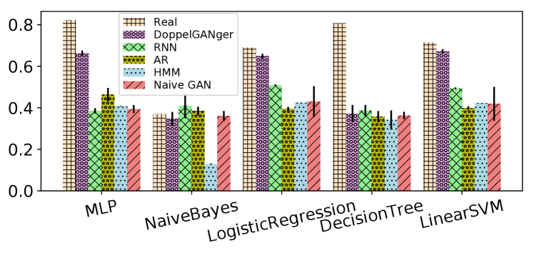
Figure 13. Event-type prediction accuracy on GCUT.

Algorithm comparison:  We evaluate whether algorithm rankings are preserved on generated data on the GCUT dataset by training different classifiers (MLP, SVM, Naive Bayes, decision tree, and logistic regression) to do end event type classification. We also evaluate this on the WWT dataset by training different regression models (MLP, linear regression, and Kernel regression) to do time series forecasting (details in Appendix D). For this use case, users have only generated data, so we want the ordering (accuracy) of algorithms on real data to be preserved when we train and test them on generated data. In other words, for each class of generated data, we train each of the predictive models on $B$ and test on $B^{\prime}$. This is different from Figure 13, where we trained on generated data ($B$) and tested on real data ($A^{\prime}$). We compare this ranking with the ground truth ranking, in which the predictive models are trained on $A$ and tested on $A^{\prime}$. We then compute the Spearman’s rank correlation coefficient (Spearman, 1904), which compares how the ranking in generated data is correlated with the groundtruth ranking. Table 5 shows that DG and AR achieve the best rank correlations. This result is misleading because AR models exhibit minimal randomness, so all predictors achieve the same high accuracy; the AR model achieves near-perfect rank correlation despite producing low-quality samples; this highlights the importance of considering rank correlation together with other fidelity metrics. More results (e.g., exact prediction numbers) are in Appendix D.

	DoppelGANger	AR	RNN	HMM	Naive GAN
GCUT	1.00	1.00	1.00	0.01	0.90
WWT	0.80	0.80	0.20	-0.60	-0.60

Table 5. Rank correlation of predication algorithms on GCUT and WWT dataset. Higher is better.

5.3. Other case studies

DG is being evaluated by several independent users, though DG has not yet been used to release any datasets to the best of our knowledge. A large public cloud provider (IBM) has internally validated the fidelity of DG. IBM stores time series data of resource usage measurements for different containers used in the cloud’s machine learning service. They trained DG to generate resource usage measurements, with the container image name as metadata. Figure 14 shows the learned distribution of containers’ maximum CPU usage (in percent). We show the maximum because developers usually size containers according to their peak usage. DG captures this challenging distribution very well, even in the heavy tail. Additionally, other users outside of the networking/systems domain such as banking, sensor data, and natural resource modeling have also been using DG (Company, 2020; Software, 2020).

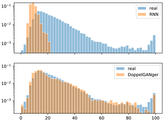
Figure 14. Maximum CPU usage.

6. Privacy Analysis and Tradeoffs

Data holders’ privacy concerns often fit in two categories: protecting business secrets (§6.1) and protecting user privacy (§6.2). In this section, we illustrate what GANs can and cannot do in each of these topics.

6.1. Protecting business secrets

In our discussions with major data holders, a primary concern about data sharing is leaking information about the types of resources available and in use at the enterprise. Many such business secrets tend to be embedded in the metadata (e.g., hardware types in a compute cluster). Note that in this case the correlation between hardware type and other metadata/measurements might be important for downstream applications, so data holders cannot simply discard hardware type from data.

There are two ways to change or obfuscate the metadata distribution. The naive way is to rejection sample the metadata to a different desired distribution. This approach is clearly inefficient. The architecture in §4.3 naturally allows data holders to obfuscate the metadata distribution in a much simpler way. After training on the original dataset, the data holders can retrain only the metadata generator to any desired distribution as the metadata generator and measurement generator are isolated. Doing so requires synthetic metadata of the desired distribution, but it does not require new time series data.

A major open question is how to realistically tune attribute distributions. Both of the above approaches to obfuscating attribute distributions keep the conditional distribution $\mathbb{P}(R^{i}|A^{i})$ unchanged, even as we alter the marginal distribution $\mathbb{P}(A^{i})$. While this may be a reasonable approximation for small perturbations, changing the marginal $\mathbb{P}(A^{i})$ may affect the conditional distribution in general. For example, $A^{i}$ may represent the fraction of large jobs in a system, and $R^{i}$ the memory usage over time; if we increase $A^{i}$, at some point we should encounter resource exhaustion. However, since the GAN is trained only on input data, it cannot predict such effects. Learning to train GANs with simulators that can model physical constraints of systems may be a good way to combine the statistical learning properties of GANs with systems that encode domain knowledge.

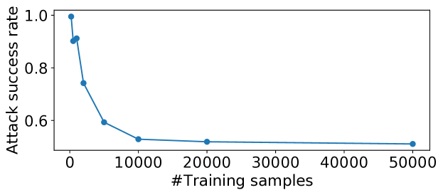
Figure 15. Membership inference attack against DG in WWT dataset vs. training set size.

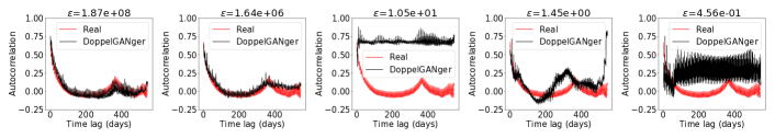
Figure 16. Autocorrelation for real and DP-GANs with different values of $\epsilon$.

6.2. Protecting user privacy

User privacy is a major concern with regards to any data sharing application, and generative models pose unique challenges. For example, recent work has shown that generative models may memorize a specific user’s information from the training data (e.g. a social security number) and leak it during data generation (Carlini et al., 2019). Hence, we need methods for evaluating and protecting user privacy. One challenge is the difficulty of defining what it means to be privacy-preserving. Although there are many competing privacy definitions (Sweeney, 2002; Dwork, 2008; Sankar et al., 2013), a common theme is deniability: released data or models should look similar whether a given user’s data is included or not.

In this section, we show how two of the most common notions of deniability relate to GANs.

Differential privacy: A leading metric for measuring user privacy today is differential privacy (DP) (Dwork, 2008). In the context of machine learning, DP states that the trained model should not depend too much on any individual user’s data. More precisely, a model $\mathcal{M}$ is $(\epsilon,\delta)$ differentially private if for any pair of training datasets $\mathcal{D}$ and $\mathcal{D}^{\prime}$ that differ in the record of a single user, and for any input $z$, it holds that

$$\mathcal{M}(z;\mathcal{D})\leq e^{\epsilon}\mathcal{M}(z;\mathcal{D}^{\prime})+\delta,$$

where $\mathcal{M}(z;\mathcal{D})$ denotes a model trained on $\mathcal{D}$ and evaluated on $z$. Smaller values of $\epsilon$ and $\delta$ give more privacy.

Recent work has explored how to make deep learning models differentially private (Abadi et al., 2016) by clipping and adding noise to the gradient updates in stochastic gradient descent to ensure that any single example in the training dataset does not disproportionately influence the model parameters. Researchers have applied this technique to GANs (Xie et al., 2018; Xu et al., 2019; Frigerio et al., 2019) to generate privacy-preserving time series (Esteban et al., 2017; Beaulieu-Jones et al., 2019); we generally call this approach DP-GAN. These papers argue that such DP-GAN architectures give privacy at minimal cost to utility. A successive paper using DP student-teacher learning achieved better performance than DP-GAN on single-shot data (Jordon et al., 2018), but we do not consider it here because its architecture is ill-suited to generating time series.

To evaluate the efficacy of DP-GANs in our context, we trained DoppelGANger with DP-GANs for the WWT dataset using TensorFlow Privacy (Andrew et al., 2019). Figure 16 shows the autocorrelation of the resulting time series for different values of the privacy budget, $\epsilon$. Smaller values of $\epsilon$ denote more privacy; $\epsilon\approx 1$ is typically considered a reasonable operating point. As $\epsilon$ is reduced (stronger privacy guarantees), autocorrelations become progressively worse. In this figure, we show results only for the 15th epoch, as the results become only worse as training proceeds (not shown). These results highlight an important point: although DP-GANs seems to destroy our autocorrelation plots, this was not always evident from downstream metrics, such as predictive accuracy in (Esteban et al., 2017). This highlights the need to evaluate generative time series models qualitatively and quantitatively; prior work has focused mainly on the latter (Esteban et al., 2017; Beaulieu-Jones et al., 2019; Jordon et al., 2018). Our results suggest that DP-GAN mechanisms require significant improvements for privacy-preserving time series generation.

Membership inference:  Another common way of evaluating user deniability is through membership inference attacks (Shokri et al., 2017; Hayes et al., 2019; Chen et al., 2019). Given a trained machine learning model and set of data samples, the goal of such an attack is to infer whether those samples were in the training dataset. The attacker does this by training a classifier to output whether each sample was in the training data. Note that differential privacy should protect against such an attack; the stronger the privacy parameter, the lower the success rate. However, DP alone does quantify the efficacy of membership inference attacks.

To understand this question further, we measure DG’s vulnerability to membership inference attacks (Hayes et al., 2019) on the WWT dataset. As in (Hayes et al., 2019), our metric is success rate, or the percentage of successful trials in guessing whether a sample is in the training dataset. Naive random guessing gives 50%, while we found an attack success rate of 51%, suggesting robustness to membership inference in this case. However, when we decrease the training set size, the attack success rate increases (Figure 15). For instance, with 200 training samples, the attack success rate is as high as 99.5%. Our results suggest a practical guideline: to be more robust against membership attacks, use more training data. This contradicts the common practice of subsetting for better privacy (Reiss et al., 2012).

Summary and implications:  The privacy properties of GANs appear to be mixed. On the positive side, GANs can be used to obfuscate attribute distributions for masking business secrets, and there appear to be simple techniques for preventing common membership inference attacks (namely, training on more data). However, the primary challenge appears to be preserving good fidelity while providing strong theoretical privacy guarantees. We find that existing approaches for providing DP destroy fidelity beyond recognition, and are not a viable solution.

More broadly, we believe there is value to exploring different privacy metrics. DP is designed for datasets where one sample corresponds to one user. However, many datasets of interest have multiple time series from the same user, and/or time series may not correspond to users at all. In these cases, DP gives hard-to-interpret guarantees, while destroying data fidelity (particularly for uncommon signal classes (Bagdasaryan et al., 2019)). Moreover, it does not defend against other attacks like model inversion (Fredrikson et al., 2014; Hitaj et al., 2017). So it is not clear whether DP is a good metric for this class of data.

7. Conclusions

While DG is a promising general workflow for data sharing, the privacy properties of GANs require further research for data holders to confidently use such workflows. Moreover, many networking datasets require significantly more complexity than DG is currently able to handle, such as causal interactions between stateful agents. Another direction of interest is to enable “what-if” analysis, in which practitioners can model changes in the underlying system and generate associated data. Although DG makes some what-if analysis easy (e.g., slightly altering the attribute distribution), larger changes may alter the physical system model such that the conditional distributions learned by DG are invalid (e.g., imagine simulating a high-traffic regime with a model trained only on low-traffic-regime data). Such what-if analysis is likely to require physical system modeling/simulation, while GANs may be able to help model individual agent behavior. We hope that the initial promise and open questions inspire further work from theoreticians and practitioners to help break the impasse in data sharing.

Data/code release and Ethics: While we highlight privacy concerns in using GAN-based models, the code/data we are releasing does not raise any ethical issues as the public datasets do not contain any personal information.

Appendix

Appendix A Datasets

Google Cluster Usage Trace:  Due to the substantial computational requirements of training GANs and our own resource constraints, we did not use the entire dataset. Instead, we uniformly sampled a subset of 100,000 tasks and used their corresponding measurement records to form our dataset. This sample was collected after filtering out the following categories:

• 197 (0.17%) tasks don’t have corresponding end events (such events may end outside the data collection period)

• 1403 (1.25%) tasks have discontinuous measurement records (i.e., the end timestamp of the previous measurement record does not equal the start timestamp of next measurement record)

• 7018 (6.25%) tasks have an empty measurement record

• 3754 (3.34%) tasks have mismatched end times (the timestamp of the end event does not match the ending timestamp of the last measurement).

The maximum measurement length in this dataset is 2497, however, 97.06% samples have length within 50. The schema of this dataset is in Table 6.

Wikipedia Web Traffic:  The original datasets consists of 145k samples. After removing samples with missing data, 117k samples are left, from which we sample 100k samples for our evaluation. All samples have measurement length 550. The schema of this dataset is in Table 7.

FCC MBA:  We used the latest cleaned data published by FCC MBA in December 2018 (Commission, 2018). This datasets contains hourly traffic measurements from 4378 homes in September and October 2017. However, a lot of measurements are missing in this dataset. Considering period from 10/01/2017 from 10/15/2017, only 45 homes have complete network usage measurements every hour. This small sample set will make us hard to understand the actual dynamic patterns in this dataset. To increase number of valid samples, we take the average of measurements every 6 hours for each home. As long as there is at least one measurement in each 6 hours period, we regard it as a valid sample. Using this way, we get 739 valid samples with measurements from 10/01/2017 from 10/15/2017, from which we sample 600 samples for our evaluation. All samples have measurement length 56. The schema of this dataset is in Table 8.

Metadata	Description	Possible Values
end event type	The reason that the task finishes	FAIL, KILL, EVICT, etc.
Measurements	Description	Possible Values
CPU rate	Mean CPU rate	float numbers
maximum CPU rate	Maximum CPU rate	float numbers
sampled CPU usage	The CPU rate sampled uniformly on all 1 second measurements	float numbers
canonical memory usage	Canonical memory usage measurement	float numbers
assigned memory usage	Memory assigned to the container	float numbers
maximum memory usage	Maximum canonical memory usage	float numbers
unmapped page cache	Linux page cache that was not mapped into any userspace process	float numbers
total page cache	Total Linux page cache	float numbers
local disk space usage	Runtime local disk capacity usage	float numbers
Timestamp Discription		Possible Values
The timestamp that the measurement was conducted on. Different task may have different number of measurement records (i.e. $T^{i}$ may be different)		2011-05-01 01:01, etc.

Table 6. Schema of GCUT dataset. Metadata and measurements are described in more detail in (Reiss et al., 2011).

Metadata	Description	Possible Values
Wikipedia domain	The main domain name of the Wikipedia page	zh.wikipedia.org, commons.wikimedia.org, etc.
access type	The access method	mobile-web, desktop, all-access, etc.
agent	The agent type	spider, all-agent, etc.
Measurements	Description	Possible Values
views	The number of views	integers
Timestamp Discription		Possible Values
The date that the page view is counted on		2015-07-01, etc.

Table 7. Schema of WWT dataset.

Metadata	Description	Possible Values
technology	The connection technology of the unit	cable, fiber, etc.
ISP	Internet service provider of the unit	AT&T, Verizon, etc.
state	The state where the unit is located	PA, CA, etc.
Measurements	Description	Possible Values
ping loss rate	UDP ping loss rate to the server that has lowest loss rate within the hour	float numbers
traffic byte counter	Total number of bytes sent and received in the hour (excluding the traffic due to the activate measurements)	integers
Timestamp Discription		Possible Values
The time of the measurement hour		2015-09-01 1:00, etc.

Table 8. Schema of MBA dataset.

Appendix B Implementation Details

DG:  Metadata generator and min/max generator are MLPs with 2 hidden layers and 100 units in each layer. Measurement generator is 1 layer of LSTM with 100 units. Softmax layer is applied for categorical measurement and metadata output. Sigmoid or tanh is applied for continuous measurement and metadata output, depending on whether data is normalized to [0,1] or [-1,1] (this is configurable). The discriminator and auxiliary discriminator are MLP with 4 hidden layers and 200 units in each layer. Gradient penalty weight was 10.0 as suggested in (Gulrajani et al., 2017). The network was trained using Adam optimizer with learning rate of 0.001 and batch size of 100 for both generators and discriminators.

Loss functions: As mentioned in §3.3.2, Wasserstein loss has been widely adopted for improving training stability and alleviating mode collapse. In our own empirical explorations, we find that Wasserstein loss is better than the original loss for generating categorical variables. Because categorical variables are prominent in our domain, we use Wasserstein loss.

In order to train the two discriminators simultaneously, we combine the loss functions of the two discriminators by a weighting parameter $\alpha$. More specifically, the loss function is

(1) $$\min_{G}\max_{D_{1},D_{2}}\mathcal{L}_{1}(G,D_{1})+\alpha\mathcal{L}_{2}(G,D_{2})$$

where $\mathcal{L}_{i}$, $i\in\{1,2\}$ is the Wasserstein loss of the original and second discriminator, respectively: $\mathcal{L}_{i}=\mathbb{E}_{x\leavevmode\nobreak\ \sim p_{x}}\left[T_{i}(D_{i}(x))\right]-\mathbb{E}_{z\sim p_{z}}\left[D_{i}(T_{i}(G(z)))\right]-\lambda\mathbb{E}_{\hat{x}\sim p_{\hat{x}}}\left[\left(\left\lVert\nabla_{\hat{x}}D_{i}(T_{i}(\hat{x}))\right\rVert_{2}-1\right)^{2}\right]$. Here $T_{1}(x)=x$ and $T_{2}(x)=$ metadata part of $x$. $\hat{x}:=tx+(1-t)G(z)$ where $t\sim\text{Unif}[0,1]$. Empirically, we find that $\alpha=1$ is enough for getting good fidelity on metadata. As with all GANs, the generator and discriminators are trained alternatively until convergence. Unlike naive GAN architectures, we did not observe problems with training instability, and on our datasets, convergence required only up to 200,000 batches (400 epochs when the number of training samples is 50,000).

Generation flag for variable lengths: Time series may have different lengths. For example, in GCUT dataset, different jobs have different duration (Figure 9). We want to learn to generate sequences of the right length organically (without requiring the user to specify it). The simplest solution to pad all time series with 0 to the same length. However, that would introduce a confusion on whether a zero value means the measurements (say, daily page view) is zero, or it is actually a padding token. Therefore, along with the original measurements, we add generation flag to each time step: $[1,0]$ if the time series does not end at this time step, and $[0,1]$ if the time series ends exactly at this time step (Figure 17). The generator outputs generation flag $[p_{1},p_{2}]$ through a softmax output layer, so that $p_{1},p_{2}\in[0,1]$ and $p_{1}+p_{2}=1$. $[p_{1},p_{2}]$ is used to determine whether we should continue unrolling the RNN to the next time step. One way to interpret this is that $p_{1}$ gives the probability that the time series should continue at this time step. Therefore, if $p_{1}<p_{2}$, we stop generation and pad all future measurements with 0’s; if $p_{1}>p_{2}$, we continue unrolling the RNN to generate measurements for the next time step(s). The generation flags are also fed to the discriminator as part of the features, so the generator can also learn sample length characteristics.

We also want to highlight that if the user wants to control the length of the generated samples, our architecture can also support this by iterating the RNN generator for the given desired number of steps.

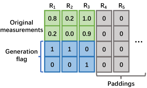
Figure 17. Generation flag for enabling variable length sequence.

AR:  We used $p=3$, i.e., used the past three samples to predict the next. The AR model was an MLP with 4 hidden layers and 200 units in each layer. The MLP was trained using Adam optimizer (Kingma and Ba, 2014) with learning rate of 0.001 and batch size of 100.

RNN:  For this baseline, we used LSTM (Long short term memory) (Hochreiter and Schmidhuber, 1997) variant of RNN. It is 1 layers of LSTM with 100 units. The network was trained using Adam optimizer with learning rate of 0.001 and batch size of 100.

Naive GAN:  The generator and discriminator are MLPs with 4 hidden layers and 200 units in each layer. Gradient penalty weight was 10.0 as suggested in (Gulrajani et al., 2017). The network was trained using Adam optimizer with learning rate of 0.001 and batch size of 100 for both generator and discriminator.

Appendix C Additional Fidelity Results

Temporal lengths:  Figure 18 shows the length distribution of DG  and baselines in GCUT dataset. It is clear that DG  has the best fidelity.

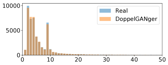
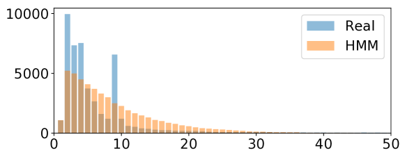
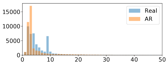
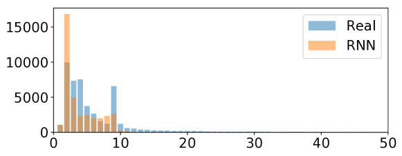
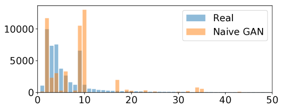
Figure 18. Histogram of task duration for the GCUT dataset. DoppelGANger gives the best fidelity.

Metadata distributions:  Figure 19 shows the histogram of Wikipedia domain of Naive GAN and DG. DG learns the distribution fairly well, whereas naive GAN cannot.

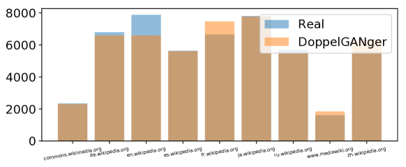
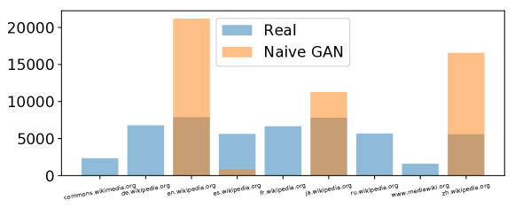
Figure 19. Histograms of Wikipedia domain from WWT dataset.

Measurement-metadata correlations:  We compute the CDF of total bandwidth for DSL and cable users in MBA dataset. Figures 20(a) and 20(b) plot the full CDFs. Most of the baselines capture the fact that cable users consume more bandwidth than DSL users. However, DG appears to excel in regions of the distribution with less data, e.g., very small bandwidth levels. In both cases, DG captures the bandwidth distribution better than the other baselines. This means that DG has a high fidelity on measurement distribution, and also successfully capture how metadata (i.e., DSL and cable) influence the measurements.

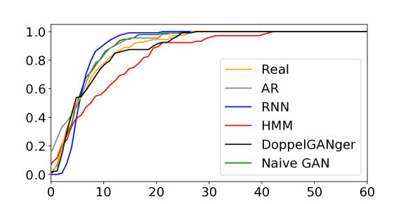
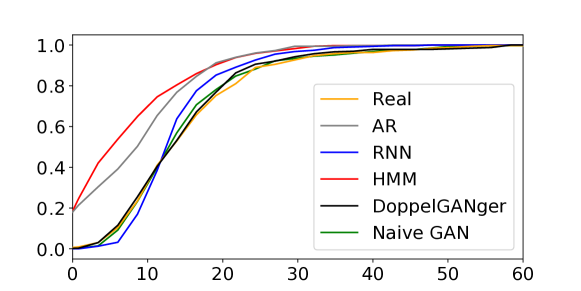
Figure 20. Total bandwidth usage in 2 weeks in MBA dataset for (a) DSL and (b) cable users.

DG does not simply memorize training samples:  Figure 21, 22, 23 show the some generated samples from DG and their nearest (based on squared error) samples in training data from the three datasets. The results show that DG is not memorizing training samples. To achieve the good fidelity results we have shown before, DG must indeed learn the underlying structure of the samples.

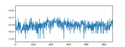
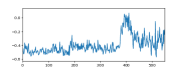
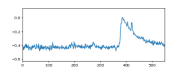
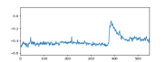
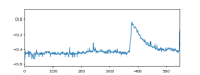
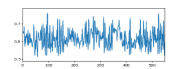
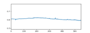
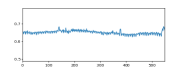
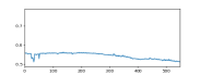
Figure 21. Three time series samples selected uniformly at random from the synthetic dataset generated using DG and the corresponding top-3 nearest neighbours (based on square error) from the real WWT dataset. The time series shown here is daily page views (normalized).

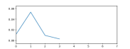
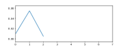
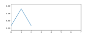
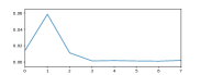
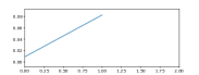
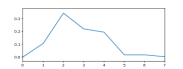
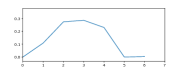
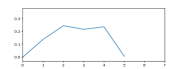
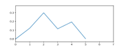
Figure 22. Three time series samples selected uniformly at random from the synthetic dataset generated using DG and the corresponding top-3 nearest neighbours (based on square error) from the real GCUT dataset. The time series shown here is CPU rate (normalized).

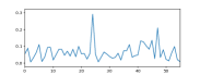
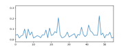
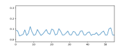
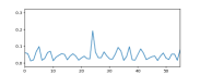
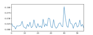
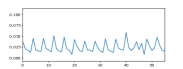
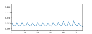
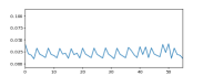
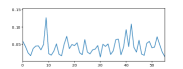
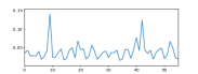
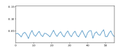
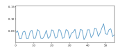
Figure 23. Three time series samples selected uniformly at random from the synthetic dataset generated using DG and the corresponding top-3 nearest neighbours (based on square error) from the real MBA dataset. The time series shown here is traffic byte counter (normalized).

Appendix D Additional Case Study Results

Predictive modeling:  For the WWT  dataset, the predictive modeling task involves forecasting of the page views for next 50 days, given those for the first 500 days. We want to learn a (relatively) parsimonious model that can take an arbitrary length-500 time series as input and predict the next 50 time steps. For this purpose, we train various regression models: an MLP with five hidden layers (200 nodes each), and MLP with just one hidden layer (100 nodes), a linear regression model, and a Kernel regression model using an RBF kernel. To evaluate each model, we compute the so-called coefficient of determination, $R^{2}$, which captures how well a regression model describes a particular dataset.

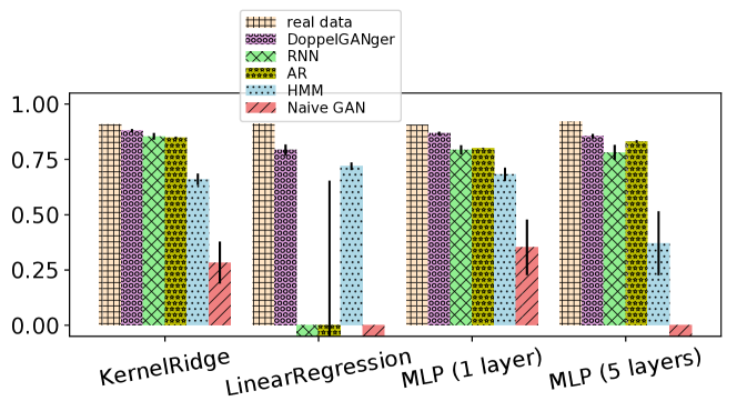
Figure 24. Coefficient of determination for WWT time series forecasting. Higher is better.

Figure 24 shows the $R^{2}$ for each of these models for each of our generative models and the real data. Here we train each regression model on generated data (B) and test it on real data (A’), hence it is to be expected that real data performs best. It is clear that DG performs better than other baselines for all regression models. Note that sometimes RNN, AR, and naive GANs baselines have large negative $R^{2}$ which are therefore not visualized in this plot.

Algorithm comparison:  Figure 25, 26 show the ranking of prediction algorithms on DG’s and baselines’ generated data. Combined with 5, we see that DG and AR are the best for preserving ranking of prediction algorithms.

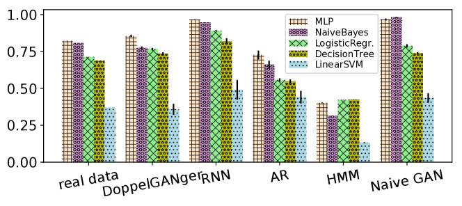
Figure 25. Ranking of end event type prediction algorithms on GCUT dataset.

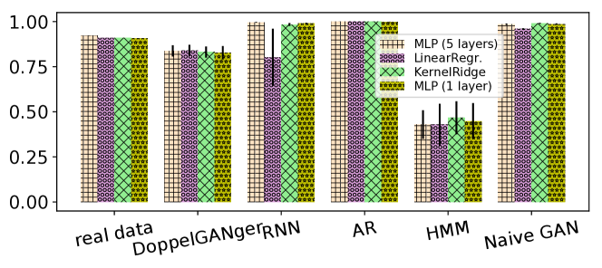
Figure 26. Ranking of traffic prediction algorithms on WWT dataset.

References

- (1)
- fio ([n. d.]) [n. d.]. FIO’s documentation. ([n. d.]). https://fio.readthedocs.io/en/latest/#
- cai ([n. d.]) [n. d.]. The internet topology data kit - 2011-04. ([n. d.]). http://www.caida.org/data/active/internet-topology-data-kit.
- Abadi et al. (2016) Martin Abadi, Andy Chu, Ian Goodfellow, H Brendan McMahan, Ilya Mironov, Kunal Talwar, and Li Zhang. 2016. Deep learning with differential privacy. In Proceedings of the 2016 ACM SIGSAC Conference on Computer and Communications Security. ACM, 308–318.
- Andrew et al. (2019) Galen Andrew, Steve Chien, and Nicolas Papernot. 2019. TensorFlow Privacy. https://github.com/tensorflow/privacy. (2019).
- Antonatos et al. (2004) Spyros Antonatos, Kostas G Anagnostakis, and Evangelos P Markatos. 2004. Generating realistic workloads for network intrusion detection systems. In Proceedings of the 4th international workshop on Software and performance. 207–215.
- Arjovsky et al. (2017) Martin Arjovsky, Soumith Chintala, and Léon Bottou. 2017. Wasserstein gan. arXiv preprint arXiv:1701.07875 (2017).
- Arora and Zhang (2017) Sanjeev Arora and Yi Zhang. 2017. Do gans actually learn the distribution? an empirical study. arXiv preprint arXiv:1706.08224 (2017).
- Backstrom et al. (2007) Lars Backstrom, Cynthia Dwork, and Jon Kleinberg. 2007. Wherefore art thou r3579x?: anonymized social networks, hidden patterns, and structural steganography. In Proceedings of the 16th international conference on World Wide Web. ACM, 181–190.
- Bagdasaryan et al. (2019) Eugene Bagdasaryan, Omid Poursaeed, and Vitaly Shmatikov. 2019. Differential privacy has disparate impact on model accuracy. In Advances in Neural Information Processing Systems. 15453–15462.
- Bai and Shi (2011) Jushan Bai and Shuzhong Shi. 2011. Estimating high dimensional covariance matrices and its applications. (2011).
- Baltrunas et al. (2014) Dziugas Baltrunas, Ahmed Elmokashfi, and Amund Kvalbein. 2014. Measuring the reliability of mobile broadband networks. In Proceedings of the 2014 Conference on Internet Measurement Conference. ACM, 45–58.
- Bauer et al. (2009) Kevin Bauer, Damon McCoy, Ben Greenstein, Dirk Grunwald, and Douglas Sicker. 2009. Physical layer attacks on unlinkability in wireless lans. In International Symposium on Privacy Enhancing Technologies Symposium. Springer, 108–127.
- Beaulieu-Jones et al. (2017) Brett K Beaulieu-Jones, Zhiwei Steven Wu, Chris Williams, and Casey S Greene. 2017. Privacy-preserving generative deep neural networks support clinical data sharing. BioRxiv (2017), 159756.
- Beaulieu-Jones et al. (2019) Brett K Beaulieu-Jones, Zhiwei Steven Wu, Chris Williams, Ran Lee, Sanjeev P Bhavnani, James Brian Byrd, and Casey S Greene. 2019. Privacy-preserving generative deep neural networks support clinical data sharing. Circulation: Cardiovascular Quality and Outcomes 12, 7 (2019), e005122.
- Benson et al. (2010) Theophilus Benson, Aditya Akella, and David A Maltz. 2010. Network traffic characteristics of data centers in the wild. In Proceedings of the 10th ACM SIGCOMM conference on Internet measurement. ACM, 267–280.
- Bischof et al. (2017) Zachary S Bischof, Fabian E Bustamante, and Nick Feamster. 2017. Characterizing and Improving the Reliability of Broadband Internet Access. arXiv preprint arXiv:1709.09349 (2017).
- Buehler et al. (2020) Hans Buehler, Blanka Horvath, Terry Lyons, Imanol Perez Arribas, and Ben Wood. 2020. A Data-driven Market Simulator for Small Data Environments. Available at SSRN 3632431 (2020).
- Cai et al. (2016) T Tony Cai, Zhao Ren, Harrison H Zhou, et al. 2016. Estimating structured high-dimensional covariance and precision matrices: Optimal rates and adaptive estimation. Electronic Journal of Statistics 10, 1 (2016), 1–59.
- Calzarossa et al. (2016) Maria Carla Calzarossa, Luisa Massari, and Daniele Tessera. 2016. Workload characterization: A survey revisited. ACM Computing Surveys (CSUR) 48, 3 (2016), 1–43.
- Carlini et al. (2019) Nicholas Carlini, Chang Liu, Úlfar Erlingsson, Jernej Kos, and Dawn Song. 2019. The secret sharer: Evaluating and testing unintended memorization in neural networks. In 28th USENIX Security Symposium (USENIX Security 19). 267–284.
- Chaisiri et al. (2011) Sivadon Chaisiri, Bu-Sung Lee, and Dusit Niyato. 2011. Optimization of resource provisioning cost in cloud computing. IEEE transactions on services Computing 5, 2 (2011), 164–177.
- Chen et al. (2019) Dingfan Chen, Ning Yu, Yang Zhang, and Mario Fritz. 2019. Gan-leaks: A taxonomy of membership inference attacks against gans. arXiv preprint arXiv:1909.03935 (2019).
- Chen et al. (2018) Li Chen, Justinas Lingys, Kai Chen, and Feng Liu. 2018. AuTO: scaling deep reinforcement learning for datacenter-scale automatic traffic optimization. In Proceedings of the 2018 Conference of the ACM Special Interest Group on Data Communication. ACM, 191–205.
- Choi et al. (2017) Edward Choi, Siddharth Biswal, Bradley Malin, Jon Duke, Walter F Stewart, and Jimeng Sun. 2017. Generating multi-label discrete patient records using generative adversarial networks. arXiv preprint arXiv:1703.06490 (2017).
- Commission (2018) Federal Communications Commission. 2018. Raw Data - Measuring Broadband America - Seventh Report. (2018). https://www.fcc.gov/reports-research/reports/measuring-broadband-america/raw-data-measuring-broadband-america-seventh.
- Company (2020) Hazy Company. 2020. Hazy builds on new technique to generate sequential and time‑series synthetic data. https://hazy.com/blog/2020/07/09/how-to-generate-sequential-data. (2020).
- Cooper et al. (2010) Brian F Cooper, Adam Silberstein, Erwin Tam, Raghu Ramakrishnan, and Russell Sears. 2010. Benchmarking cloud serving systems with YCSB. In Proceedings of the 1st ACM symposium on Cloud computing. 143–154.
- De Meer, Fernando (2019) De Meer, Fernando. 2019. Generating Financial Series with Generative Adversarial Networks. (2019).
- Denneulin et al. (2004) Yves Denneulin, Emmanuel Romagnoli, and Denis Trystram. 2004. A synthetic workload generator for cluster computing. In 18th International Parallel and Distributed Processing Symposium, 2004. Proceedings. IEEE, 243.
- Di and Cappello (2015) Sheng Di and Franck Cappello. 2015. GloudSim: Google trace based cloud simulator with virtual machines. Software: Practice and Experience 45, 11 (2015), 1571–1590.
- Di et al. (2014) Sheng Di, Derrick Kondo, and Franck Cappello. 2014. Characterizing and modeling cloud applications/jobs on a Google data center. The Journal of Supercomputing 69, 1 (2014), 139–160.
- Dong et al. (2018) Hao-Wen Dong, Wen-Yi Hsiao, Li-Chia Yang, and Yi-Hsuan Yang. 2018. Musegan: Multi-track sequential generative adversarial networks for symbolic music generation and accompaniment. In Thirty-Second AAAI Conference on Artificial Intelligence.
- Dwork (2008) Cynthia Dwork. 2008. Differential privacy: A survey of results. In International Conference on Theory and Applications of Models of Computation. Springer, 1–19.
- Esteban et al. ([n. d.]) Cristóbal Esteban, Stephanie L Hyland, and Gunnar Rätsch. [n. d.]. RCGAN code repository. ([n. d.]). https://github.com/ratschlab/RGAN.
- Esteban et al. (2017) Cristóbal Esteban, Stephanie L Hyland, and Gunnar Rätsch. 2017. Real-valued (medical) time series generation with recurrent conditional GANs. arXiv preprint arXiv:1706.02633 (2017).
- Fedus et al. (2018) William Fedus, Ian Goodfellow, and Andrew M Dai. 2018. MaskGAN: better text generation via filling in the_. arXiv preprint arXiv:1801.07736 (2018).
- Forsati and Meybodi (2010) Rana Forsati and Mohammad Reza Meybodi. 2010. Effective page recommendation algorithms based on distributed learning automata and weighted association rules. Expert Systems with Applications 37, 2 (2010), 1316–1330.
- Fredrikson et al. (2014) Matthew Fredrikson, Eric Lantz, Somesh Jha, Simon Lin, David Page, and Thomas Ristenpart. 2014. Privacy in pharmacogenetics: An end-to-end case study of personalized warfarin dosing. In 23rd USENIX Security Symposium (USENIX Security 14). 17–32.
- Frid-Adar et al. (2018) Maayan Frid-Adar, Eyal Klang, Michal Amitai, Jacob Goldberger, and Hayit Greenspan. 2018. Synthetic data augmentation using GAN for improved liver lesion classification. In 2018 IEEE 15th international symposium on biomedical imaging (ISBI 2018). IEEE, 289–293.
- Frigerio et al. (2019) Lorenzo Frigerio, Anderson Santana de Oliveira, Laurent Gomez, and Patrick Duverger. 2019. Differentially Private Generative Adversarial Networks for Time Series, Continuous, and Discrete Open Data. In IFIP International Conference on ICT Systems Security and Privacy Protection. Springer, 151–164.
- Fu et al. (2019) Rao Fu, Jie Chen, Shutian Zeng, Yiping Zhuang, and Agus Sudjianto. 2019. Time Series Simulation by Conditional Generative Adversarial Net. arXiv preprint arXiv:1904.11419 (2019).
- Fu and Xu (2007) Song Fu and Cheng-Zhong Xu. 2007. Exploring event correlation for failure prediction in coalitions of clusters. In Proceedings of the 2007 ACM/IEEE conference on Supercomputing. ACM, 41.
- Ganapathi et al. (2010) Archana Ganapathi, Yanpei Chen, Armando Fox, Randy Katz, and David Patterson. 2010. Statistics-driven workload modeling for the cloud. In 2010 IEEE 26th International Conference on Data Engineering Workshops (ICDEW 2010). IEEE, 87–92.
- González et al. (2005) Alicia Mateo González, AM Son Roque, and Javier García-González. 2005. Modeling and forecasting electricity prices with input/output hidden Markov models. IEEE Transactions on Power Systems 20, 1 (2005), 13–24.
- Goodfellow (2016) Ian Goodfellow. 2016. NIPS 2016 tutorial: Generative adversarial networks. arXiv preprint arXiv:1701.00160 (2016).
- Goodfellow et al. (2014) Ian Goodfellow, Jean Pouget-Abadie, Mehdi Mirza, Bing Xu, David Warde-Farley, Sherjil Ozair, Aaron Courville, and Yoshua Bengio. 2014. Generative adversarial nets. In Advances in neural information processing systems. 2672–2680.
- Google (2018) Google. 2018. Web Traffic Time Series Forecasting. (2018). https://www.kaggle.com/c/web-traffic-time-series-forecasting.
- Grandl et al. (2015) Robert Grandl, Ganesh Ananthanarayanan, Srikanth Kandula, Sriram Rao, and Aditya Akella. 2015. Multi-resource packing for cluster schedulers. ACM SIGCOMM Computer Communication Review 44, 4 (2015), 455–466.
- Guibas et al. (2017) John T Guibas, Tejpal S Virdi, and Peter S Li. 2017. Synthetic medical images from dual generative adversarial networks. arXiv preprint arXiv:1709.01872 (2017).
- Gulrajani et al. (2017) Ishaan Gulrajani, Faruk Ahmed, Martin Arjovsky, Vincent Dumoulin, and Aaron C Courville. 2017. Improved training of wasserstein gans. In Advances in Neural Information Processing Systems. 5767–5777.
- Halevy et al. (2009) Alon Halevy, Peter Norvig, and Fernando Pereira. 2009. The unreasonable effectiveness of data. IEEE Intelligent Systems 24, 2 (2009), 8–12.
- Han et al. (2018) Changhee Han, Hideaki Hayashi, Leonardo Rundo, Ryosuke Araki, Wataru Shimoda, Shinichi Muramatsu, Yujiro Furukawa, Giancarlo Mauri, and Hideki Nakayama. 2018. GAN-based synthetic brain MR image generation. In 2018 IEEE 15th International Symposium on Biomedical Imaging (ISBI 2018). IEEE, 734–738.
- Hayes et al. (2019) Jamie Hayes, Luca Melis, George Danezis, and Emiliano De Cristofaro. 2019. LOGAN: Membership Inference Attacks Against Generative Models. Proceedings on Privacy Enhancing Technologies 2019, 1 (2019), 133–152.
- He et al. (2013) Keqiang He, Alexis Fisher, Liang Wang, Aaron Gember, Aditya Akella, and Thomas Ristenpart. 2013. Next stop, the cloud: Understanding modern web service deployment in ec2 and azure. In Proceedings of the 2013 conference on Internet measurement conference. ACM, 177–190.
- Heusel et al. (2017) Martin Heusel, Hubert Ramsauer, Thomas Unterthiner, Bernhard Nessler, and Sepp Hochreiter. 2017. Gans trained by a two time-scale update rule converge to a local nash equilibrium. In Advances in neural information processing systems. 6626–6637.
- Hinton et al. (2012) Geoffrey Hinton, Nitish Srivastava, and Kevin Swersky. 2012. Neural networks for machine learning lecture 6a overview of mini-batch gradient descent. (2012). http://www.cs.toronto.edu/~hinton/coursera/lecture6/lec6.pdf.
- Hitaj et al. (2017) Briland Hitaj, Giuseppe Ateniese, and Fernando Perez-Cruz. 2017. Deep models under the GAN: information leakage from collaborative deep learning. In Proceedings of the 2017 ACM SIGSAC Conference on Computer and Communications Security. 603–618.
- Hochreiter and Schmidhuber (1997) Sepp Hochreiter and Jürgen Schmidhuber. 1997. Long short-term memory. Neural computation 9, 8 (1997), 1735–1780.
- Issariyakul and Hossain (2009) Teerawat Issariyakul and Ekram Hossain. 2009. Introduction to network simulator 2 (NS2). In Introduction to network simulator NS2. Springer, 1–18.
- Jiang et al. (2016a) Junchen Jiang, Rajdeep Das, Ganesh Ananthanarayanan, Philip A Chou, Venkata Padmanabhan, Vyas Sekar, Esbjorn Dominique, Marcin Goliszewski, Dalibor Kukoleca, Renat Vafin, et al. 2016a. Via: Improving internet telephony call quality using predictive relay selection. In Proceedings of the 2016 ACM SIGCOMM Conference. ACM, 286–299.
- Jiang et al. (2016b) Junchen Jiang, Vyas Sekar, Henry Milner, Davis Shepherd, Ion Stoica, and Hui Zhang. 2016b. CFA: A Practical Prediction System for Video QoE Optimization.. In NSDI. 137–150.
- Jordon et al. ([n. d.]) James Jordon, Daniel Jarrett, Jinsung Yoon, Paul Elbers, Patrick Thoral, Ari Ercole, Cheng Zhang, Danielle Belgrave, and Mihaela van der Schaar. [n. d.]. NeurIPS 2020 hide-and-seek privacy challenge. https://www.vanderschaar-lab.com/privacy-challenge/. ([n. d.]).
- Jordon et al. (2018) James Jordon, Jinsung Yoon, and Mihaela van der Schaar. 2018. PATE-GAN: Generating synthetic data with differential privacy guarantees. (2018).
- Juan et al. (2014) Da-Cheng Juan, Lei Li, Huan-Kai Peng, Diana Marculescu, and Christos Faloutsos. 2014. Beyond poisson: Modeling inter-arrival time of requests in a datacenter. In Pacific-Asia Conference on Knowledge Discovery and Data Mining. Springer, 198–209.
- Karras et al. (2017) Tero Karras, Timo Aila, Samuli Laine, and Jaakko Lehtinen. 2017. Progressive growing of gans for improved quality, stability, and variation. arXiv preprint arXiv:1710.10196 (2017).
- Kingma and Ba (2014) Diederik P Kingma and Jimmy Ba. 2014. Adam: A method for stochastic optimization. arXiv preprint arXiv:1412.6980 (2014).
- Li and Li (2009) Tiancheng Li and Ninghui Li. 2009. On the tradeoff between privacy and utility in data publishing. In Proceedings of the 15th ACM SIGKDD international conference on Knowledge discovery and data mining. ACM, 517–526.
- Li and Liu (2014) Ting Li and Jason Liu. 2014. Cluster-based spatiotemporal background traffic generation for network simulation. ACM Transactions on Modeling and Computer Simulation (TOMACS) 25, 1 (2014), 1–25.
- Li et al. (2018) Zhijing Li, Zihui Ge, Ajay Mahimkar, Jia Wang, Ben Y Zhao, Haitao Zheng, Joanne Emmons, and Laura Ogden. 2018. Predictive Analysis in Network Function Virtualization. In Proceedings of the Internet Measurement Conference 2018. ACM, 161–167.
- Lin et al. (2018) Zinan Lin, Ashish Khetan, Giulia Fanti, and Sewoong Oh. 2018. PacGAN: The power of two samples in generative adversarial networks. In Advances in Neural Information Processing Systems. 1505–1514.
- Liu et al. (2017) Ning Liu, Zhe Li, Jielong Xu, Zhiyuan Xu, Sheng Lin, Qinru Qiu, Jian Tang, and Yanzhi Wang. 2017. A hierarchical framework of cloud resource allocation and power management using deep reinforcement learning. In ICDCS. IEEE, 372–382.
- Lucic et al. (2018) Mario Lucic, Karol Kurach, Marcin Michalski, Sylvain Gelly, and Olivier Bousquet. 2018. Are gans created equal? a large-scale study. In Advances in neural information processing systems. 700–709.
- Magalhães et al. (2015) Deborah Magalhães, Rodrigo N Calheiros, Rajkumar Buyya, and Danielo G Gomes. 2015. Workload modeling for resource usage analysis and simulation in cloud computing. Computers & Electrical Engineering 47 (2015), 69–81.
- Mao et al. (2016) Hongzi Mao, Mohammad Alizadeh, Ishai Menache, and Srikanth Kandula. 2016. Resource management with deep reinforcement learning. In Proceedings of the 15th ACM Workshop on Hot Topics in Networks. ACM, 50–56.
- Maqableh et al. (2014) Mahmoud Maqableh, Huda Karajeh, et al. 2014. Job scheduling for cloud computing using neural networks. Communications and Network 6, 03 (2014), 191.
- Marti (2020) Gautier Marti. 2020. CorrGAN: Sampling Realistic Financial Correlation Matrices Using Generative Adversarial Networks. In ICASSP 2020-2020 IEEE International Conference on Acoustics, Speech and Signal Processing (ICASSP). IEEE, 8459–8463.
- McGregor et al. (2010) Tony McGregor, Shane Alcock, and Daniel Karrenberg. 2010. The RIPE NCC internet measurement data repository. In International Conference on Passive and Active Network Measurement. Springer, 111–120.
- Melamed (1993) Benjamin Melamed. 1993. An overview of TES processes and modeling methodology. In Performance Evaluation of Computer and Communication Systems. Springer, 359–393.
- Melamed and Hill (1993) Benjamin Melamed and Jon R Hill. 1993. Applications of the TES modeling methodology. In Proceedings of 1993 Winter Simulation Conference-(WSC’93). IEEE, 1330–1338.
- Melamed et al. (1992) Benjamin Melamed, Jon R Hill, and David Goldsman. 1992. The TES methodology: Modeling empirical stationary time series. In Proceedings of the 24th conference on Winter simulation. ACM, 135–144.
- Melamed and Pendarakis (1998) Benjamin Melamed and Dimitrios E Pendarakis. 1998. Modeling full-length VBR video using Markov-renewal-modulated TES models. IEEE Journal on Selected Areas in Communications 16, 5 (1998), 600–611.
- Mogren (2016) Olof Mogren. 2016. C-RNN-GAN: Continuous recurrent neural networks with adversarial training. arXiv preprint arXiv:1611.09904 (2016).
- Montazeri et al. (2018) Behnam Montazeri, Yilong Li, Mohammad Alizadeh, and John Ousterhout. 2018. Homa: A Receiver-Driven Low-Latency Transport Protocol Using Network Priorities. In SIGCOMM.
- Moreno et al. (2014) Ismael Solis Moreno, Peter Garraghan, Paul Townend, and Jie Xu. 2014. Analysis, modeling and simulation of workload patterns in a large-scale utility cloud. IEEE Transactions on Cloud Computing 2, 2 (2014), 208–221.
- Narayanan and Shmatikov (2008) Arvind Narayanan and Vitaly Shmatikov. 2008. Robust de-anonymization of large sparse datasets. In Security and Privacy, 2008. SP 2008. IEEE Symposium on. IEEE, 111–125.
- Nguyen et al. (2013) Thi Thanh Sang Nguyen, Hai Yan Lu, and Jie Lu. 2013. Web-page recommendation based on web usage and domain knowledge. IEEE Transactions on Knowledge and Data Engineering 26, 10 (2013), 2574–2587.
- Nystrom et al. (2015) Nicholas A. Nystrom, Michael J. Levine, Ralph Z. Roskies, and J. Ray Scott. 2015. Bridges: A Uniquely Flexible HPC Resource for New Communities and Data Analytics. In Proceedings of the 2015 XSEDE Conference: Scientific Advancements Enabled by Enhanced Cyberinfrastructure (XSEDE ’15). ACM, New York, NY, USA, Article 30, 8 pages. https://doi.org/10.1145/2792745.2792775
- Odena et al. (2017) Augustus Odena, Christopher Olah, and Jonathon Shlens. 2017. Conditional image synthesis with auxiliary classifier gans. In Proceedings of the 34th International Conference on Machine Learning-Volume 70. JMLR. org, 2642–2651.
- Ohm (2009) Paul Ohm. 2009. Broken promises of privacy: Responding to the surprising failure of anonymization. Ucla L. Rev. 57 (2009), 1701.
- Reiss et al. (2011) Charles Reiss, John Wilkes, and Joseph L Hellerstein. 2011. Google cluster-usage traces: format+ schema. Google Inc., White Paper (2011), 1–14.
- Reiss et al. (2012) Charles Reiss, John Wilkes, and Joseph L Hellerstein. 2012. Obfuscatory obscanturism: making workload traces of commercially-sensitive systems safe to release. In 2012 IEEE Network Operations and Management Symposium. IEEE, 1279–1286.
- Salimans et al. (2016) Tim Salimans, Ian Goodfellow, Wojciech Zaremba, Vicki Cheung, Alec Radford, and Xi Chen. 2016. Improved techniques for training gans. In Advances in Neural Information Processing Systems. 2234–2242.
- Sankar et al. (2013) Lalitha Sankar, S Raj Rajagopalan, and H Vincent Poor. 2013. Utility-privacy tradeoffs in databases: An information-theoretic approach. IEEE Transactions on Information Forensics and Security 8, 6 (2013), 838–852.
- Shokri et al. (2017) Reza Shokri, Marco Stronati, Congzheng Song, and Vitaly Shmatikov. 2017. Membership inference attacks against machine learning models. In 2017 IEEE Symposium on Security and Privacy (SP). IEEE, 3–18.
- Sliwko and Getov (2016) Leszek Sliwko and Vladimir Getov. 2016. AGOCS—Accurate Google Cloud Simulator Framework. In 2016 Intl IEEE Conferences on Ubiquitous Intelligence & Computing, Advanced and Trusted Computing, Scalable Computing and Communications, Cloud and Big Data Computing, Internet of People, and Smart World Congress (UIC/ATC/ScalCom/CBDCom/IoP/SmartWorld). IEEE, 550–558.
- Software (2020) Boogie Software. 2020. Synthesizing series of transactions with a Generative Adversarial Network. https://blog.boogiesoftware.com/2020/02/synthesizing-series-of-transactions.html. (2020).
- Sommers and Barford (2004) Joel Sommers and Paul Barford. 2004. Self-configuring network traffic generation. In Proceedings of the 4th ACM SIGCOMM conference on Internet measurement. ACM, 68–81.
- Sommers et al. (2011) Joel Sommers, Rhys Bowden, Brian Eriksson, Paul Barford, Matthew Roughan, and Nick Duffield. 2011. Efficient network-wide flow record generation. In 2011 Proceedings IEEE INFOCOM. IEEE, 2363–2371.
- Sommers et al. (2004) Joel Sommers, Vinod Yegneswaran, and Paul Barford. 2004. A framework for malicious workload generation. In Proceedings of the 4th ACM SIGCOMM conference on Internet measurement. 82–87.
- Spearman (1904) Charles Spearman. 1904. The proof and measurement of association between two things. American journal of Psychology 15, 1 (1904), 72–101.
- Srivastava et al. (2017) Akash Srivastava, Lazar Valkov, Chris Russell, Michael U Gutmann, and Charles Sutton. 2017. Veegan: Reducing mode collapse in gans using implicit variational learning. In Advances in Neural Information Processing Systems. 3308–3318.
- Srivastava et al. (2000) Jaideep Srivastava, Robert Cooley, Mukund Deshpande, and Pang-Ning Tan. 2000. Web usage mining: Discovery and applications of usage patterns from web data. Acm Sigkdd Explorations Newsletter 1, 2 (2000), 12–23.
- Srivatsa and Hicks (2012) Mudhakar Srivatsa and Mike Hicks. 2012. Deanonymizing mobility traces: Using social network as a side-channel. In Proceedings of the 2012 ACM conference on Computer and communications security. 628–637.
- Sundaresan et al. (2017) Srikanth Sundaresan, Xiaohong Deng, Yun Feng, Danny Lee, and Amogh Dhamdhere. 2017. Challenges in inferring internet congestion using throughput measurements. In Proceedings of the 2017 Internet Measurement Conference. ACM, 43–56.
- Sweeney (2000) Latanya Sweeney. 2000. Simple demographics often identify people uniquely. Health (San Francisco) 671 (2000), 1–34.
- Sweeney (2002) Latanya Sweeney. 2002. k-anonymity: A model for protecting privacy. International Journal of Uncertainty, Fuzziness and Knowledge-Based Systems 10, 05 (2002), 557–570.
- Tarasov et al. (2016) Vasily Tarasov, Erez Zadok, and Spencer Shepler. 2016. Filebench: A flexible framework for file system benchmarking. USENIX; login 41, 1 (2016), 6–12.
- Towns et al. (2014) J. Towns, T. Cockerill, M. Dahan, I. Foster, K. Gaither, A. Grimshaw, V. Hazlewood, S. Lathrop, D. Lifka, G. D. Peterson, R. Roskies, J. R. Scott, and N. Wilkins-Diehr. 2014. XSEDE: Accelerating Scientific Discovery. Computing in Science Engineering 16, 5 (2014), 62–74.
- Vishwanath and Vahdat (2009) Kashi Venkatesh Vishwanath and Amin Vahdat. 2009. Swing: Realistic and responsive network traffic generation. IEEE/ACM Transactions on Networking (TON) 17, 3 (2009), 712–725.
- Weigle et al. (2006) Michele C Weigle, Prashanth Adurthi, Félix Hernández-Campos, Kevin Jeffay, and F Donelson Smith. 2006. Tmix: a tool for generating realistic TCP application workloads in ns-2. ACM SIGCOMM Computer Communication Review 36, 3 (2006), 65–76.
- Williams and Zipser (1989) Ronald J Williams and David Zipser. 1989. A learning algorithm for continually running fully recurrent neural networks. Neural computation 1, 2 (1989), 270–280.
- Xie et al. (2018) Liyang Xie, Kaixiang Lin, Shu Wang, Fei Wang, and Jiayu Zhou. 2018. Differentially private generative adversarial network. arXiv preprint arXiv:1802.06739 (2018).
- Xu et al. (2019) Chugui Xu, Ju Ren, Deyu Zhang, Yaoxue Zhang, Zhan Qin, and Kui Ren. 2019. GANobfuscator: Mitigating information leakage under GAN via differential privacy. IEEE Transactions on Information Forensics and Security 14, 9 (2019), 2358–2371.
- Xu et al. (2018) Qiantong Xu, Gao Huang, Yang Yuan, Chuan Guo, Yu Sun, Felix Wu, and Kilian Weinberger. 2018. An empirical study on evaluation metrics of generative adversarial networks. arXiv preprint arXiv:1806.07755 (2018).
- Yin et al. (2014) Jianwei Yin, Xingjian Lu, Xinkui Zhao, Hanwei Chen, and Xue Liu. 2014. BURSE: A bursty and self-similar workload generator for cloud computing. IEEE Transactions on Parallel and Distributed Systems 26, 3 (2014), 668–680.
- Yoon ([n. d.]) Jinsung Yoon. [n. d.]. TimeGAN code repository. ([n. d.]). https://bitbucket.org/mvdschaar/mlforhealthlabpub/src/02edab3b2b6d635470fa80184bbfd03b8bf8082d/alg/timegan/.
- Yoon et al. (2019) Jinsung Yoon, Daniel Jarrett, and Mihaela van der Schaar. 2019. Time-series Generative Adversarial Networks. In Advances in Neural Information Processing Systems. 5509–5519.
- Yu et al. (2017) Lantao Yu, Weinan Zhang, Jun Wang, and Yong Yu. 2017. SeqGAN: Sequence Generative Adversarial Nets with Policy Gradient.. In AAAI. 2852–2858.
- Zec et al. (2019) Edvin Listo Zec, Henrik Arnelid, and Nasser Mohammadiha. 2019. Recurrent Conditional GANs for Time Series Sensor Modelling. In Time Series Workshop at International Conference on Machine Learning,(Long Beach, California).