Stationary scalar hairy configurations supported by Neumann compact stars

Abstract

Abstract

We study stationary scalar field hairy configurations supported by asymptotically flat horizonless compact stars. At the star surface, we impose Neumann boundary conditions for the scalar field. With analytical methods, we obtain bounds on the frequency of scalar fields. For certain discrete frequency satisfying the bounds, we numerically get solutions of scalar hairy stars. We also disclose effects of model parameters on the discrete frequency of scalar fields.

I Introduction

The no hair theorem, see e.g. Bekenstein -JBN , plays an important role in the development of black hole theories. The classical no hair theorem states that asymptotically flat black holes cannot support scalars, massive vectors and Abelian Higgs hairs outside the horizon, for recent progress see mr1 -CW and reviews see Bekenstein-1 ; CAR . It was believed that the no hair property is mainly due to the existence of absorbing horizons.

Recently, it was found that such no hair behaviors also appear in spacetimes without horizons. Hod firstly proved that static massive scalar fields cannot exist outside asymptotically flat horizonless neutral compact stars, which are endowed with scalar reflecting surface boundary conditions Hod-6 . With static scalar fields non-minimally coupled to the gravity, asymptotically flat horizonless neutral reflecting compact stars still cannot support static scalar field hairs nonm1 ; nonm2 ; nonm3 . No static scalar hair theorem also holds for horizonless neutral reflecting compact stars with a nonzero cosmological constant Bhattacharjee ; Yan Peng-1 ; Yan Peng-3 . Then what is the case when the compact star is charged. It was found that no static scalar hair theorem holds for large charged asymptotic flat horizonless reflecting compact stars and in contrast, static scalar hair can form outside small charged asymptotic flat horizonless reflecting compact stars Hod-8 -Yan Peng-8 . Very differently, asymptotically flat charged black holes cannot support scalar hairs cbh1 ; cbh2 . If we want to obtain static scalar hairs outside asymptotically flat charged black holes, we usually have to put the black hole in a box Dolan ; Basu ; Oscar ; Sanchis ; blc1 ; blc2 .

From above progress, it seems that no static scalar field hair behavior is a general property in the neutral horizonless reflecting compact stars. Theoretically, the scalar field can be either static or stationary. So it is also interesting to examine whether stationary scalar fields can condense outside neutral horizonless compact stars. In the background of black holes, stationary scalar hairs can exist when the spacetime is rotating Hod-1 -st11 . In contrast, for horizonless compact reflecting stars, Hod showed that non-rotating neutral star can support exterior stationary scalar field hairs Stationary . Instabilities of compact stars with Neumann boundary conditions were also numerically investigated in Maggio . One naturally wonders whether this instability can trigger scalar hairs outside Neumann compact stars. In this work, we plan to examine whether stationary scalar fields can condense outside neutral horizonless Neumann compact stars, where we impose Neumann boundary conditions instead of Dirichlet reflecting conditions in Stationary .

In the following, we introduce the system composed of stationary scalar fields and neutral horizonless Neumann compact stars. We analytically obtain bounds on the frequency of stationary scalar hairs. We also numerically get stationary hairy neutral horizonless Neumann compact stars. We summarize main results in the last section.

II Bounds on the frequency of stationary scalar fields

We consider the possible configuration with exterior stationary scalar fields outside compact stars. And the corresponding matter field Lagrange density is given by

$$\mathcal{L}=-|\nabla_{\mu}\Psi|^{2}-m^{2}\Psi^{2}.$$ (1)

Here $\Psi$ is the stationary scalar field and m corresponds to the scalar field mass.

In Schwarzschild coordinates, the spacetime outside the compact star is described by metric

$$ds^{2} = -f(r)dt^{2}+\frac{dr^{2}}{f(r)}+r^{2}(d\theta^{2}+sin^{2}\theta d\phi^{2}),$$ (2)

where $f(r)$ is the metric function. We take the radial coordinate $r=r_{s}$ as the radius of the star surface. Outside the surface, it is the Schwarzschild type solution $f(r)=1-\frac{2M}{r}$, where M is the star mass. Since we focus on horizonless star, there is the relation $r_{s}>2M$. $\theta$ and $\phi$ are angular coordinates.

The scalar field equation is ISP ; ISPY ; metric3

$$(\nabla^{\nu}\nabla_{\nu}-m^{2})\Psi=0.$$ (3)

We study stationary scalar fields expressed in the simple form

$$\Psi(t,r)=e^{-i\omega t}\psi(r)$$ (4)

with $\omega$ as the frequency.

Then the equation (3) can be expressed as

$$\psi^{\prime\prime}+(\frac{2}{r}+\frac{f^{\prime}}{f})\psi^{\prime}+(\frac{\omega^{2}}{f^{2}}-\frac{m^{2}}{f})\psi=0$$ (5)

with $f=1-\frac{2M}{r}$.

At the surface, we impose the Neumann condition for the scalar field in the form $\psi^{\prime}(r_{s})=0$. At the infinity, the general asymptotic behavior for the bounded scalar field is BC

$$\psi\sim\frac{1}{r}e^{-\sqrt{m^{2}-\omega^{2}}r}.$$ (6)

So the scalar field satisfies boundary conditions

$$\psi^{\prime}(r_{s})=0,~{}~{}~{}~{}~{}~{}~{}~{}~{}~{}~{}~{}~{}\psi(\infty)=0.$$ (7)

With a new radial function $\tilde{\psi}=\sqrt{r}\psi$, the scalar field equation (5) can be transformed into

$$r^{2}\tilde{\psi}^{\prime\prime}+(r+\frac{r^{2}f^{\prime}}{f})\tilde{\psi}^{\prime}+(-\frac{1}{4}-\frac{rf^{\prime}}{2f}+\frac{\omega^{2}r^{2}}{f^{2}}-\frac{m^{2}r^{2}}{f})\tilde{\psi}=0$$ (8)

with $f=1-\frac{2M}{r}$.

Boundary conditions of the function $\tilde{\psi}$ are

$$\tilde{\psi}^{\prime}(r_{s})=\frac{1}{2\sqrt{r_{s}}}\psi(r_{s})+\sqrt{r_{s}}\psi^{\prime}(r_{s})=\frac{1}{2\sqrt{r_{s}}}\psi(r_{s})=\frac{1}{2r_{s}}\tilde{\psi}(r_{s}),$$ (9)

$$\tilde{\psi}\sim\frac{1}{\sqrt{r}}e^{-\sqrt{m^{2}-\omega^{2}}r}\rightarrow 0~{}~{}~{}as~{}~{}~{}r\rightarrow\infty.$$ (10)

In the following, we divide our discussion into three cases: $\tilde{\psi}(r_{s})=0$, $\tilde{\psi}(r_{s})>0$ and $\tilde{\psi}(r_{s})<0$.

In the first case of $\tilde{\psi}(r_{s})=0$, considering the relation (10), at least one extremum point $r_{peak}$ of $\tilde{\psi}(r)$ exists between the surface and the infinity boundary. The extremum point may be positive maximum extremum point satisfying

$$\tilde{\psi}(r_{peak})>0,\tilde{\psi}^{\prime}(r_{peak})=0,\tilde{\psi}^{\prime\prime}(r_{peak})\leqslant 0$$ (11)

or negative minimum extremum point with

$$\tilde{\psi}(r_{peak})<0,\tilde{\psi}^{\prime}(r_{peak})=0,\tilde{\psi}^{\prime\prime}(r_{peak})\geqslant 0.$$ (12)

In the second case of $\tilde{\psi}(r_{s})>0$, there is $\tilde{\psi}^{\prime}(r_{s})=\frac{1}{2r_{s}}\tilde{\psi}(r_{s})>0$. Around the star surface, the positive scalar field firstly increases to be larger and approaches zero at the infinity. So one positive maximum extremum point $r_{peak}$ exists. At this maximum extremum point, we have the relation

$$\tilde{\psi}(r_{peak})>0,\tilde{\psi}^{\prime}(r_{peak})=0,\tilde{\psi}^{\prime\prime}(r_{peak})\leqslant 0.$$ (13)

In the third case of $\tilde{\psi}(r_{s})<0$, there is $\tilde{\psi}^{\prime}(r_{s})=\frac{1}{2r_{s}}\tilde{\psi}(r_{s})<0$. Around the star surface, the negative scalar field firstly decreases to be more negative and approaches zero at the infinity. So one negative minimum extremum point $r_{peak}$ exists. At this minimum extremum point, we have the relation

$$\tilde{\psi}(r_{peak})<0,\tilde{\psi}^{\prime}(r_{peak})=0,\tilde{\psi}^{\prime\prime}(r_{peak})\geqslant 0.$$ (14)

As a summary of (11-14), scalar field solutions satisfy characteristic relations

$$\{\tilde{\psi}^{\prime}=0~{}~{}~{}~{}and~{}~{}~{}~{}\tilde{\psi}\tilde{\psi}^{\prime\prime}\leqslant 0\}~{}~{}~{}~{}for~{}~{}~{}~{}r=r_{peak}.$$ (15)

From (8), we get the equation

$$r^{2}\tilde{\psi}\tilde{\psi}^{\prime\prime}+(r+\frac{r^{2}f^{\prime}}{f})\tilde{\psi}\tilde{\psi}^{\prime}+(-\frac{1}{4}-\frac{rf^{\prime}}{2f}+\frac{\omega^{2}r^{2}}{f^{2}}-\frac{m^{2}r^{2}}{f})\tilde{\psi}^{2}=0.$$ (16)

Relations (15) and (16) lead to the inequality

$$-\frac{1}{4}-\frac{rf^{\prime}}{2f}+\frac{\omega^{2}r^{2}}{f^{2}}-\frac{m^{2}r^{2}}{f}\geqslant 0~{}~{}~{}for~{}~{}~{}r=r_{peak}.$$ (17)

With $f(r)=1-\frac{2M}{r}$, (17) can be transformed into

$$\frac{1}{r^{2}}-\frac{8m^{2}M}{r}+4(m^{2}-\omega^{2})\leqslant 0~{}~{}~{}for~{}~{}~{}r=r_{peak}.$$ (18)

(18) yields the relation

$$(\frac{1}{r}-4m^{2}M)^{2}+4(m^{2}-\omega^{2})-16m^{4}M^{2}\leqslant 0~{}~{}~{}for~{}~{}~{}r=r_{peak}.$$ (19)

From (19), we obtain the inequality

$$4(m^{2}-\omega^{2})-16m^{4}M^{2}\leqslant 0.$$ (20)

It yields the bound for the frequency as

$$\frac{\omega^{2}}{m^{2}}\geqslant 1-4m^{2}M^{2}.$$ (21)

According to (18), there is

$$-\frac{8m^{2}M}{r}+4(m^{2}-\omega^{2})\leqslant 0~{}~{}~{}for~{}~{}~{}r=r_{peak}.$$ (22)

From (22), we get the relation

$$\frac{\omega^{2}}{m^{2}}\geqslant 1-\frac{2M}{r_{peak}}\geqslant 1-\frac{2M}{r_{s}}.$$ (23)

According to the infinity asymptotic behavior (6), the bound-state fields are characterized by proper resonant frequencies with the relation Hod-9

$$m^{2}\geqslant\omega^{2}.$$ (24)

With (21), (23) and (24), we obtain bounds on the frequency as

$$max\{1-\frac{2M}{r_{s}},1-4m^{2}M^{2}\}\leqslant\frac{\omega^{2}}{m^{2}}\leqslant 1.$$ (25)

In the limit of $r_{s}\gg M$, for fixed nonzero $mM$, (25) is the same as Hod’s bound Stationary

$$1-\frac{2M}{r_{s}}\leqslant\frac{\omega^{2}}{m^{2}}\leqslant 1.$$ (26)

For ultra-compact star, $r_{s}$ can be chosen a little larger than 2M. In the limit $r_{s}\rightarrow 2M$, (25) is equal to

$$1-4m^{2}M^{2}\leqslant\frac{\omega^{2}}{m^{2}}\leqslant 1.$$ (27)

III Stationary scalar configurations supported by neutral Neumann compact stars

The stationary scalar hairy compact stars were analytically studied in the limit of $M\ll r_{s}$, where the Dirichlet reflecting conditions were imposed at the star surface Stationary . With numerical methods, we carry out the discussion in the case of relaxing the condition $M\ll r_{s}$. In this work, we try to search for stationary scalar hairy compact stars with Neumann surface boundary conditions.

Since the equation (5) is of the second order, we need values $\psi(r_{s})$, $\psi^{\prime}(r_{s})$ and model parameters to integrate the equation. We choose to describe the system with dimensionless quantity $mr_{s}$, $mM$ and $\frac{\omega}{m}$ according to the symmetry of the equation (5) in the form

$$r\rightarrow kr,~{}~{}~{}~{}m\rightarrow m/k,~{}~{}~{}~{}M\rightarrow kM,~{}~{}~{}~{}\omega\rightarrow\omega/k.$$ (28)

Neumann surface boundary conditions yield $\psi^{\prime}(r_{s})=0$. Using the symmetry $\psi\rightarrow k\psi$ of the equation (5), we can fix $\psi(r_{s})=1$. For fixed $mr_{s}$ and $mM$, we can search for the proper $\frac{\omega}{m}$ satisfying the infinity boundary condition $\psi(\infty)=0$.

With given values of $mr_{s}$ and $mM$, we obtain discrete $\frac{\omega}{m}$ satisfying the infinity boundary condition. For example, for $mr_{s}=5$ and $mM=1.5$, we find $\frac{\omega}{m}$ is around 0.91654092 satisfying the bounds (25). Now we plot the scalar field solution with $mr_{s}=5$, $mM=1.5$ and $\frac{\omega}{m}=0.91654092$ in the left panel of Fig. 1. As shown in the picture, the scalar field satisfying Neumann conditions at the star surface and asymptotically approaches zero at the infinity. In addition, for $mr_{s}=5$, $mM=1.5$ and $\frac{\omega}{m}=0.96407075$, we obtain configurations with nodes and plotted it in the right panel of Fig. 1. In fact, we can also get configurations with many nodes. In black hole backgrounds, configurations without nodes are usually thermodynamically more stable compared to configurations with nodes st1 ; st2 . In this work, we focus on configurations without nodes. We will try to examine stability of such horizonless configurations with nodes in the next work.

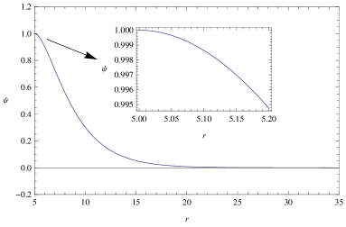
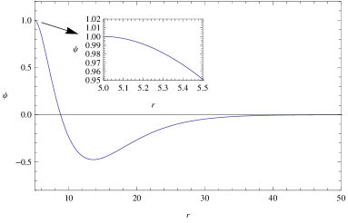
Figure 1: (Color online) We plot the scalar field function $\psi$ with respect to the radial coordinate $r$ in the case of $mr_{s}=5$ and $mM=1.5$. The left panel is with $\frac{\omega}{m}=0.91654092$ and the right panel corresponds to $\frac{\omega}{m}=0.96407075$.

In the limit of $r_{s}\gg M$, according to the bounds (26), the numerical value of the frequency should be almost 1. In this work, since we relax the condition $r_{s}\gg M$, the numerical value of the frequency can be away from 1. In the following, we study the frequency of the stationary scalar hair. In Table I, we show cases with $mr_{s}=5$ and various $mM$. We find that $\frac{\omega}{m}$ decreases as a function of $mM$. In Table II, with $mM=1.5$ and various $mr_{s}$, it can be easily seen that the frequency $\frac{\omega}{m}$ increases with respect to $mr_{s}$. We also mention that effects of parameters on the frequency is qualitatively the same as cases with Dirichlet conditions in the limit $r_{s}\gg M$ Stationary .

Table 1: The frequency $\frac{\omega}{m}$ with $mr_{s}=5$ and various $mM$

$~{}mM~{}$	0.5	1.0	1.5	2.0	2.5
$~{}\frac{\omega}{m}~{}$	0.98315836	0.95300241	0.91654092	0.87691533	0.84537691

Table 2: The frequency $\frac{\omega}{m}$ with $mM=1.5$ and various $mr_{s}$

$~{}mr_{s}~{}$	4	5	6	7	8
$~{}\frac{\omega}{m}~{}$	0.90082899	0.91654092	0.92813679	0.93681321	0.94352675

We give a physical discussion about the dependences given in Table I and II. The scalar field equation (5) can be expressed in the following form

$$\psi^{\prime\prime}+(\frac{2}{r}+\frac{f^{\prime}}{f})\psi^{\prime}-(m^{2}-\frac{\omega^{2}}{f})\frac{\psi}{f}=0.$$ (29)

From equation (29), the effective scalar field mass is defined as $m^{2}_{eff}=m^{2}-\frac{\omega^{2}}{f}=m^{2}(1-\frac{\frac{\omega^{2}}{m^{2}}}{1-\frac{2M}{r}})$. It is known that negative scalar field mass usually makes the scalar field easier to condense st1 . We show that the effective scalar field mass could be negative around the star surface. A negative effective scalar field mass around the star may trigger the scalar field field to condense. At the infinity, the effective scalar field mass asymptotically approaches a nonnegative value $m^{2}-\omega^{2}\geqslant 0$, which could serve as a potential to confine scalar field hairs Sanchis . At the star surface $r=r_{s}$, the effective scalar field mass is $\tilde{m}^{2}_{eff}=m^{2}(1-\frac{\frac{\omega^{2}}{m^{2}}}{1-\frac{2M}{r_{s}}})$. In horizonless spacetimes, there is $0<1-\frac{2M}{r_{s}}<1$. For fixed $1-\frac{2M}{r_{s}}$, a large enough $\frac{\omega^{2}}{m^{2}}$ leads to a negative $\tilde{m}^{2}_{eff}$. With larger mM and fixed $mr_{s}$, $f(r_{s})=1-\frac{2M}{r_{s}}=1-\frac{2mM}{mr_{s}}$ decreases and we need a smaller $\frac{\omega^{2}}{m^{2}}$ to get the negative $\tilde{m}^{2}_{eff}$. In the case of larger $mr_{s}$ and fixed mM, $f(r_{s})=1-\frac{2M}{r_{s}}=1-\frac{2mM}{mr_{s}}$ increases and we need a larger $\frac{\omega^{2}}{m^{2}}$ to get the negative $\tilde{m}^{2}_{eff}$. So it is natural that the frequency $\frac{\omega}{m}$ may decrease with increasing mM and increase with increasing $mr_{s}$, as is shown by numerical data in Table I and II.

IV Conclusions

We studied the gravity model composed of stationary scalar fields and horizonless neutral compact stars in the asymptotically flat background. We imposed Neumann surface boundary conditions for scalar fields. We analytically obtained bounds on the frequency of stationary scalar field as $max\{1-\frac{2M}{r_{s}},1-4m^{2}M^{2}\}\leqslant\frac{\omega^{2}}{m^{2}}\leqslant 1$, were $\omega$ is the scalar field frequency, m is the scalar field mass, M cooresponds to the star mass and $r_{s}$ represents star radii. Below the bottom bound or above the upper bound, stationary scalar hairs cannot form outside horizonless Neumann compact stars. For certain discrete frequency between the bounds, we numerically obtained solutions of stationary scalar hairy Neumann compact stars. We also investigated effects of model parameters on the discrete scalar field frequency.

- (1) J. D. Bekenstein, Transcendence of the law of baryon-number conservation in black hole physics, Phys. Rev. Lett. 28(1972)452.
- (2) J. E. Chase, Event horizons in Static Scalar-Vacuum Space-Times, Commun. Math. Phys. 19(1970)276.
- (3) C. Teitelboim, Nonmeasurability of the baryon number of a black-hole, Lett. Nuovo Cimento 3(1972)326.
- (4) R. Ruffini and J. A. Wheeler, Introducing the black hole, Phys. Today 24(1971)30.
- (5) W.K.H. Panofsky, Needs Versus Means In High-energy Physics, Phys. Today 33(1980)24-33.
- (6) M. Heusler, A No hair theorem for selfgravitating nonlinear sigma models, J. Math. Phys. 33(1992)3497-3502.
- (7) Markus Heusler, A Mass bound for spherically symmetric black hole space-times, Class. Quant. Grav. 12(1995)779-790.
- (8) J.D. Bekenstein, Novel “no-scalar-hair” theorem for black holes, Phys. Rev. D 51(1995)no.12,R6608.
- (9) D. Nez, H. Quevedo, and D. Sudarsky,Black Holes Have No Short Hair, Phys. Rev. Lett. 76(1996)571.
- (10) S. Hod, Hairy Black Holes and Null Circular Geodesics, Phys. Rev. D 84(2011)124030.
- (11) C. L. Benone, L. C. B. Crispino, C. Herdeiro, and E. Radu, Kerr-Newman scalar clouds, Phys. Rev. D 90(2014)104024.
- (12) Yan Peng, Hair mass bound in the black hole with non-zero cosmological constants, Phys. Rev. D 98(2018)104041.
- (13) J. C. Degollado and C. A. R. Herdeiro, Stationary scalar configurations around extremal charged black holes, Gen. Rel. Grav. 45(2013)2483.
- (14) Eugeny Babichev, Christos Charmousis, Dressing a black hole with a time-dependent Galileon, JHEP 1408(2014)106.
- (15) Y. Brihaye, C. Herdeiro, and E. Radu, Inside black holes with synchronized hair, Phys. Lett. B 760(2016)279.
- (16) Thomas P. Sotiriou, Shuang-Yong Zhou, Black hole hair in generalized scalar- tensor gravity, Phys. Rev. Lett. 112(2014)251102.
- (17) M. Khodaei, H. Mohseni Sadjadi, No skyrmion hair for stationary spherically symmetric reflecting stars, Phys. Lett. B 797(2019)134922.
- (18) Carlos A.R. Herdeiro, Eugen Radu, Nicolas Sanchis-Gual, José A. Font, Spontaneous Scalarization of Charged Black Holes, Phys. Rev. Lett. 121(2018)no.10,101102.
- (19) S. Hod, Spontaneous scalarization of Gauss-Bonnet black holes: Analytic treatment in the linearized regime, Phys. Rev. D 100(2019)no.6,064039.
- (20) C. Herdeiro, I. Perapechka, E. Radu, Ya. Shnir, Asymptotically flat spinning scalar, Dirac and Proca stars, Phys. Lett. B 797(2019)134845.
- (21) Pedro V.P. Cunha, Carlos A.R. Herdeiro, Eugen Radu, Spontaneously Scalarized Kerr Black Holes in Extended Scalar-Tensor-Gauss-Bonnet Gravity, Phys. Rev. Lett. 123(2019)no.1,011101.
- (22) Pedro V.P. Cunha, Carlos A.R. Herdeiro, Eugen Radu, EHT constraint on the ultralight scalar hair of the M87 supermassive black hole, arXiv:1909.08039[gr-qc].
- (23) Yves Brihaye, Betti Hartmann, Spontaneous scalarization of charged black holes at the approach to extremality, Phys. Lett. B 792(2019)244-250.
- (24) Shuang-Qing Wu, Dan Wen, Qing-Quan Jiang, Shu-Zheng Yang, Thermodynamics of five-dimensional static three-charge STU black holes with squashed horizons, Phys. Lett. B 726(2013)404-407.
- (25) Shuang-Qing Wu, Shoulong Li, Thermodynamics of Static Dyonic AdS Black Holes in the -Deformed Kaluza-Klein Gauged Supergravity Theory, Phys. Lett. B 746(2015)276-280.
- (26) Shuang-Qing Wu, Di Wu, Thermodynamical hairs of the 4-dimensional Taub-Newman-Unti-Tamburino spacetimes, arXiv:1909.07776[hep-th].
- (27) Carlos Herdeiro, Eugen Radu, Helgi Runarsson, Kerr black holes with Proca hair, Class.Quant.Grav. 33(2016)no.15,154001.
- (28) J. D. Bekenstein, Black hole hair: 25-years after, arXiv:gr-qc/9605059.
- (29) Carlos A. R. Herdeiro, Eugen Radu,Asymptotically flat black holes with scalar hair: a review, Int. J. Mod. Phys. D 24(2015)09,1542014.
- (30) S.Hod, No-scalar-hair theorem for spherically symmetric reflecting stars, Phys. Rev. D 94(2016)104073.
- (31) Shahar Hod, No hair for spherically symmetric neutral reflecting stars: Nonminimally coupled massive scalar fields, Phys. Lett. B 773(2017)208-212.
- (32) Shahar Hod, No nonminimally coupled massless scalar hair for spherically symmetric neutral reflecting stars, Phys. Rev. D 96(2017)024019.
- (33) Avraham E. Mayo, Jacob D. Bekenstein, No hair for spherical black holes: Charged and nonminimally coupled scalar field with selfinteraction, Phys. Rev. D 54(1996)5059-5069.
- (34) Srijit Bhattacharjee, Sudipta Sarkar, No-hair theorems for a static and stationary reflecting star, Phys. Rev. D 95(2017)084027.
- (35) Yan Peng, Bin Wang, Yunqi Liu, Scalar field condensation behaviors around reflecting shells in Anti-de Sitter spacetimes, Eur. Phys. J. C 78(2018) no.8,680.
- (36) Yan Peng, Static scalar field condensation in regular asymptotically AdS reflecting star backgrounds, Phys. Lett. B 782(2018)717-722.
- (37) S.Hod, Charged massive scalar field configurations supported by a spherically symmetric charged reflecting shell, Phys. Lett. B 763(2016)275.
- (38) S.Hod, Marginally bound resonances of charged massive scalar fields in the background of a charged reflecting shell, Phys. Lett. B 768(2017)97-102.
- (39) Yan Peng, Scalar field configurations supported by charged compact reflecting stars in a curved spacetime, Phys. Lett. B 780(2018)144-148.
- (40) Shahar Hod, Charged reflecting stars supporting charged massive scalar field configurations, Eur. Phys. J. C 78(2017)173.
- (41) Yan Peng, No hair theorem for bound-state massless static scalar fields outside horizonless Neumann compact stars, Phys. Lett. B 796(2019)65-67.
- (42) S. Hod, Stability of the extremal Reissner-Nordstrm black hole to charged scalar perturbations, Physics Letters B 713(2012)505.
- (43) S. Hod,No-bomb theorem for charged Reissner-Nordstrm black holes,Physics Letters B 718(2013)1489.
- (44) S. R. Dolan, S. Ponglertsakul, E. Winstanley, Stability of black holes in Einstein-charged scalar field theory in a cavity, Phys. Rev. D 92(2015)no.12,124047.
- (45) Pallab Basu, Chethan Krishnan, P. N. Bala Subramanian, Hairy Black Holes in a Box, JHEP 1611(2016)041.
- (46) Oscar J. C. Dias, Ramon Masachs, Evading no-hair theorems: hairy black holes in a Minkowski box, Phys. Rev. D 97(2018)no.12,124030.
- (47) N. Sanchis-Gual, J. C. Degollado, P. J. Montero, J. A. Font and C. Herdeiro, Explosion and Final State of an Unstable Reissner-Nordström Black Hole, Phys. Rev. Lett. 116(2016)no.14,141101.
- (48) Yan Peng,Studies of a general flat space/boson star transition model in a box through a language similar to holographic superconductors, JHEP 07(2017)042.
- (49) Yan Peng, Bin Wang, Yunqi Liu, On the thermodynamics of the black hole and hairy black hole transitions in the asymptotically flat spacetime with a box, Eur. Phys. J. C 78(2018)no.3,176.
- (50) S. Hod,Stationary Scalar Clouds Around Rotating Black Holes, Phys. Rev. D 86(2012)104026.
- (51) C. A. R. Herdeiro and E. Radu,Kerr black holes with scalar hair, Phys. Rev. Lett. 112(2014)221101.
- (52) P. V. P. Cunha, C. A. R. Herdeiro, E. Radu, and H. F. Rnarsson, Shadows of Kerr black holes with scalar hair, Phys. Rev. Lett. 115(2015)211102.
- (53) Carlos Herdeiro, Eugen Radu,Construction and physical properties of Kerr black holes with scalar hair, Class. Quant. Grav. 32(2015)no.14,144001.
- (54) Shahar Hod, Kerr-Newman black holes with stationary charged scalar clouds, Phys. Rev. D 90(2014)no.2,024051.
- (55) Shahar Hod,The large-mass limit of cloudy black holes,Class. Quant. Grav. 32(2015)no.13,134002.
- (56) Yan Peng, The extreme orbital period in scalar hairy kerr black holes, Phys. Lett. B 792(2019)1-3.
- (57) Jorge F.M. Delgado, Carlos A.R. Herdeiro, Eugen Radu, Kerr black holes with synchronised scalar hair and higher azimuthal harmonic index, Phys. Lett. B 792(2019)436-444.
- (58) Yong-Qiang Wang, Yu-Xiao Liu, Shao-Wen Wei,Excited Kerr black holes with scalar hair, Phys. Rev. D 99(2019)064036.
- (59) Shahar Hod, Stationary bound-state massive scalar field configurations supported by spherically symmetric compact reflecting stars, Eur. Phys. J. C 77(2017)899.
- (60) Elisa Maggio, Paolo Pani, Valeria Ferrari, Exotic Compact Objects and How to Quench their Ergoregion Instability, Phys. Rev. D 96(2017) no.10,104047.
- (61) S. Chandrasekhar, The Mathematical Theory of Black Holes, (Oxford University Press, New York, 1983).
- (62) S. Hod,Upper bound on the gravitational masses of stable spatially regular charged compact objects, Phys. Rev. D 98(2018)064014.
- (63) Yan Peng, On instabilities of scalar hairy regular compact reflecting stars, JHEP 1810(2018)185.
- (64) H. Bondi,Anisotropic spheres in general relativity, Mon. Not. R. Astron. Soc. 259(1992)365.
- (65) Shahar Hod, No hair for spherically symmetric neutral black holes: Nonminimally coupled massive scalar fields, Phys. Rev. D 96(2017)124037.
- (66) Yan Peng and Yunqi Liu, A general holographic metal/superconductor phase transition model, JHEP 02(2015)082.
- (67) Daniela D. Doneva and Stoytcho S. Yazadjiev, New Gauss-Bonnet Black Holes with Curvature-Induced Scalarization in Extended Scalar-Tensor Theories, Phys. Rev. Lett. 120(2018)131103.