Geometry along Evolution of Mixed Quantum States

Abstract

The metric underlying the mixed state geometric phase in unitary and nonunitary evolution [Phys. Rev. Lett. 85, 2845 (2000); Phys. Rev. Lett. 93, 080405 (2004)] is delineated. An explicit form for the line element is derived and shown to be related to an averaged energy dispersion in the case of unitary evolution. The line element is measurable in interferometry involving nearby internal states. Explicit geodesics are found in the single qubit case. It is shown how the Bures line element can be obtained by extending our approach to arbitrary decompositions of density operators. The proposed metric is applied to a generic magnetic system in a thermal state.

I Introduction

A quantum-mechanical metric underlies the notion of statistical distance that measures the distinguishability of quantum states wootters81 ; braunstein94 . Such measures can be used to quantify quantum entanglement shimony95 ; vedral97 ; wei03 , but have also found applications in the study of quantum phase transitions venuti07 ; you07 . Similarly, the related concept of path length has been used to find time-optimal curves in quantum state spaces carlini06 and to establish the speed-limit of quantum evolution margolus98 ; deffner13 ; mondal16 .

Like the geometric phase (GP), the metric is closely related to the ray structure of quantum states. To each form of GP there is a corresponding metric. For pure states, the GP is the Aharonov-Anandan phase aharonov87 with the corresponding Fubini-Study metric provost80 ; anandan90 , both arising from the horizontal lift to the one-dimensional rays over the quantum state space. For mixed states, the GP can be taken as the Uhlmann holonomy uhlmann86 with the corresponding Bures metric hubner92 both arising from the horizontal lift to the possible decompositions of density operators. The horizontal lifts guarantee that the geometric quantities are properties of state space.

The mixed state geometric phase (GP) in unitary sjoqvist00 and nonunitary tong04 evolution has been proposed as an alternative to Uhlmann’s holonomy along paths of density operators. A key point of the mixed state GP is that it is operational in the sense that it is directly accessible in interferometry. Indeed, it has been studied on different experimental platforms du03 ; ericsson05 ; klepp08 . Although the mixed state GP is now a well-established concept in a wide range of contexts, the physics of the corresponding metric andersson19 has not been explored so far. The intention of the present work is to fill this gap.

To understand the conceptual basis of our approach, we note that the corresponding mixed state GP in the case of unitary evolution reads sjoqvist00

$$\Phi_{g}=\arg\sum_{k}p_{k}e^{i\beta_{k}}$$ (1)

with $p_{k}$ and $e^{i\beta_{k}}$ being eigenvalues and eigenstate GP factors, respectively, of the evolving density operator $\rho$. In other words, the spectral decomposition of $\rho$ plays a central role. Therefore, the corresponding metric must fundamentally be based on a distance for spectral decompositions of density operators. Here, we describe how such a metric can be designed. We further discuss various applications of this metric as well as its relation to the Bures’ metric.

II Derivation of line element

Consider a smooth path $t\mapsto\rho(t)$ of density operators representing the evolving state of a quantum system. We shall assume that all non-zero eigenvalues of $\rho(t)$ are non-degenerate. In this way, the gauge freedom in the spectral decomposition is the phase of the eigenvectors; thus, a non-degenerate density operator $\rho(t)$, assumed to have rank $N$, is in one to one correspondence with the $N$ orthogonal rays $\{e^{if_{k}(t)}|n_{k}(t)\rangle|f_{k}(t)\in[0,2\pi)\}$. To capture this, we let

$$\mathcal{B}(t)=\left\{\sqrt{p_{k}(t)}e^{if_{k}(t)}|n_{k}(t)\rangle\right\}_{n=1}^{N}$$ (2)

represent the spectral decompositions along the path. We further assume that all $f_{k}(t)$ are once differentiable.

We propose the line element connecting two nearby points to be the minimum of the distance

$$d^{2}(t,t+dt)=\sum_{k}\left|\left|\sqrt{p_{k}(t)}e^{if_{k}(t)}|n_{k}(t)\rangle\right.\right.$$

$$\left.\left.-\sqrt{p_{k}(t+dt)}e^{if_{k}(t+dt)}|n_{k}(t+dt)\rangle\right|\right|^{2}.$$ (3)

To find this minimum, we expand the squares yielding

$$d^{2}(t,t+dt)$$ (4)

$$= 2-2\sum_{k}\sqrt{p_{k}(t)p_{k}(t+dt)}\Big{|}\langle n_{k}(t)|n_{k}(t+dt)\rangle\Big{|}$$

$$\times\cos\lambda_{k}(t,t+dt),$$

where $\lambda_{k}(t,t+dt)=\dot{f}_{k}(t)dt+\arg\left[1+\langle n_{k}(t)|\dot{n}_{k}(t)\rangle dt\right]+{\rm O}(dt^{2})$. The line element is thus given by

$$ds^{2}=d_{\min}^{2}(t,t+dt)$$ (5)

$$= 2-2\sum_{k}\sqrt{p_{k}(t)p_{k}(t+dt)}\Big{|}\langle n_{k}(t)|n_{k}(t+dt)\rangle\Big{|},$$

being reached when all $\lambda_{k}(t,t+dt)$ vanish to first order in $dt$, which is equivalent to

$$\dot{f}_{k}(t)-i\langle n_{k}(t)|\dot{n}_{k}(t)\rangle=0,$$ (6)

for all $k$. Equation (6) is precisely the connection underlying the mixed state GP sjoqvist00 , itself a direct extension of the Aharonov-Anandan connection for pure states aharonov87 . The connection provides the necessary link between the mixed state GP sjoqvist00 and the metric concept considered here. Equation (5) can be put on a more useful form by expanding to lowest non-trivial order in $dt$. We suppress the $t$ argument (for notational simplicity) and make use of the identities $\langle n_{k}|\ddot{n}_{k}\rangle+\langle\ddot{n}_{k}|n_{k}\rangle=-2\langle\dot{n}_{k}|\dot{n}_{k}\rangle$ and $\sum_{k}\dot{p}_{k}=\sum_{k}\ddot{p}_{k}=0$, which follow from the normalization conditions $\langle n_{k}|n_{k}\rangle=1$ and $\sum_{k}p_{k}=1$. We find

$$ds^{2}=\sum_{k}p_{k}ds_{k}^{2}+\frac{1}{4}\sum_{k}\frac{dp_{k}^{2}}{p_{k}},$$ (7)

where

$$ds_{k}^{2}=\langle\dot{n}_{k}|\left(\hat{1}-|n_{k}\rangle\langle n_{k}|\right)|\dot{n}_{k}\rangle dt^{2}$$ (8)

is the pure state Fubini-Study metric (infinitesimal line element) along $|n_{k}\rangle$ provost80 and $dp_{k}=\dot{p}_{k}dt$. Note the structural similarity between the first term of the right-hand side of Eq. (7) and the expression for the mixed state GP in Eq. (1), both being weighted sums of the corresponding pure state quantities. The second term we recognize as the Fischer-Rao information metric for classical probability distributions bengtsson06 . In the following, we shall examine various applications of the line element in Eq. (7).

III Applications

III.1 Unitary evolution, time-energy uncertainty

Let us first consider the case of unitary time evolution $i\hbar\dot{\rho}=[H,\rho]$ governed by some Hamiltonian $H$. Here, the Fischer-Rao term vanishes since the probability weights $p_{k}$ are constant. By using the geometric time-energy relation in Ref. anandan90 , we find

$$ds^{2}=\frac{1}{\hbar^{2}}\overline{\Delta E}^{2}dt^{2},$$ (9)

with the mixed state energy dispersion $\overline{\Delta E}^{2}=\sum_{k}p_{k}\left(\Delta_{k}E\right)^{2}$. Here, $\Delta_{k}E$ is the energy dispersion of $|n_{k}\rangle$. Thus, the speed by which the eigendecomposition of the density operator changes along the path is $ds/dt=(1/\hbar)\overline{\Delta E}$ .

Note that the energy dispersion $\overline{\Delta E}^{2}$ is different from the standard quantum-mechanical dispersion $\Delta_{\rho}E^{2}={\rm Tr}(\rho H^{2})-[{\rm Tr}(\rho H)]^{2}$. However, the inequality

$$\overline{\Delta E}^{2}\leq\Delta_{\rho}E^{2}$$ (10)

relates the two. To prove this, we note that $\overline{\Delta E}^{2}$ and $\Delta_{\rho}E^{2}$ are independent of zero-point energy and are therefore unchanged under the shift $H\rightarrow\widetilde{H}\equiv H-{\rm Tr}(\rho H)$. We find $\Delta_{\rho}E^{2}={\rm Tr}(\rho\widetilde{H}^{2})$ and thus $\overline{\Delta E}^{2}={\rm Tr}(\rho\widetilde{H}^{2})-\sum_{k}p_{k}\langle n_{k}|\widetilde{H}|n_{k}\rangle^{2}=\Delta_{\rho}E^{2}-\sum_{k}p_{k}\langle n_{k}|\widetilde{H}|n_{k}\rangle^{2}$, which implies Eq. (10) since $\sum_{k}p_{k}\langle n_{k}|\widetilde{H}|n_{k}\rangle^{2}\geq 0$.

A time-energy uncertainty relation similar to those of Refs. anandan90 ; uhlmann92 can be formulated. Consider two unitarily connected states and assume $s_{\min}$ is the shortest distance between them, as measured by $ds$ in Eq. (7). Let $\langle\overline{\Delta E}\rangle=(1/\Delta t)\int_{0}^{\Delta t}\overline{\Delta E}dt$ and $\langle\Delta_{\rho}E\rangle=(1/\Delta t)\int_{0}^{\Delta t}\Delta_{\rho}Edt$ be the time-averaged energy dispersions for the traversal time $\Delta t$ between the two states. Equation (9) combined with Eq. (10) implies

$$\langle\Delta_{\rho}E\rangle\Delta t\geq\langle\overline{\Delta E}\rangle\Delta t\geq s_{\min}\hbar,$$ (11)

which provides a geometric lower bound for the energy-time uncertainty. This geometric bound is apparently tighter for $\langle\overline{\Delta E}\rangle$ than for $\langle\Delta_{\rho}E\rangle$.

III.2 Interferometry

We now address the operational significance of the line element $ds^{2}$. In the unitary case, the proposed line element can be related to measurable quantities by using the technique of Ref. sjoqvist00 . Consider a Mach-Zehnder interferometer with a pair of 50-50 beam-splitters acting as $|x\rangle\mapsto 2^{-1/2}\big{[}|x\rangle+(-1)^{x}|x\oplus 1\rangle\big{]}$ on the beam states $x=0,1$, and $\rho$ describing the ‘internal’ state of the particles injected into the interferometer.

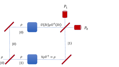
Figure 1: Interferometer to measure the line element induced by the unitary $U(\delta t)$ in the $|0\rangle$ beam. The reference beam $|1\rangle$ is exposed to a unitary $V$ that commutes with the internal input state $\rho$. Its role is to maximize the output probability $P_{0}$ in the horizontal beam. To leading non-trivial order in $\delta t$, one has $P_{0}=1-\frac{1}{4}\delta s^{2}$, which gives direct experimental access to the line element for a small but finite time $\delta t$.

Assume the input state $|0\rangle\langle 0|\otimes\rho$ hits the first beam-splitter followed by a unitary $|0\rangle\langle 0|\otimes U(\delta t)+|1\rangle\langle 1|\otimes V$, $\delta t$ being a small but finite time interval and $[V,\rho]=0$. Thus, in the $0$-beam the internal state undergoes the transformation $\rho\mapsto U(\delta t)\rho U^{\dagger}(\delta t)$, while it remains unchanged in the $1$-beam: $\rho\mapsto V\rho V^{\dagger}=\rho$, see Fig. 1. By writing $V=\sum_{k}e^{if_{k}}|n_{k}\rangle\langle n_{k}|$, we obtain the probabilities

$$P_{0}=1-P_{1}=\frac{1}{2}+\frac{1}{2}{\rm Re}\sum_{k}p_{k}\langle n_{k}|U(\delta t)|n_{k}\rangle e^{-if_{k}}$$ (12)

to find the particles in the two beams after passing the second beam-splitter. We write $U(\delta t)=\hat{1}-\frac{i}{\hbar}H\delta t-\frac{1}{2\hbar^{2}}H^{2}\delta t^{2}+\ldots$, where $H$ is the Hamiltonian acting on the internal degrees of freedom of the particles, and maximize $P_{0}$ over each of the phases $f_{k}$, yielding to lowest non-trivial order in $\delta t$

$$P_{0,\max}=\max_{\{f_{k}\}}P_{0}=1-\frac{1}{4}\delta s^{2}.$$ (13)

Here, $\delta s^{2}=\frac{1}{\hbar^{2}}\overline{\Delta E}^{2}\delta t^{2}$ is Eq. (9) for a finite but small time interval.

In order to generalize the interferometric setting to the non-unitary case, the purification-based technique described in Ref. tong04 can be used. That is, one adds an auxiliary system and prepare the combined system in a pure internal input state $|\Psi\rangle=\sum_{k}\sqrt{p_{k}}|n_{k}\rangle\otimes|a_{k}\rangle$ with $\langle a_{k}|a_{l}\rangle=\delta_{kl}$, thus satisfying $\rho={\rm Tr}_{a}|\Psi\rangle\langle\Psi|$. Now, the above unitary that is applied between the beam-splitters is replaced by the extended unitary $|0\rangle\langle 0|\otimes W(\delta t)+|1\rangle\langle 1|\otimes V\otimes\hat{1}_{a}$. Here, $W(\delta t)$ acts on the combined system as $W(\delta t)|\Psi\rangle=\sum_{k}\sqrt{p_{k}+\delta p_{k}}U(\delta t)|n_{k}\rangle\otimes|a_{k}\rangle$, while $V\otimes\hat{1}_{a}|\Psi\rangle=\sum_{k}e^{if_{k}}\sqrt{p_{k}}|n_{k}\rangle\otimes|a_{k}\rangle$. The reduced states in the two beams undergo the transformations $\rho\mapsto U(\delta t)\sum_{k}(p_{k}+\delta p_{k})|n_{k}\rangle\langle n_{k}|U^{\dagger}(\delta t)$ and $\rho\mapsto V\rho V^{\dagger}=\rho$. By superposing the two beams at the second beam-splitter, we obtain the output state

$$|\Psi_{\rm out}\rangle \propto \sum_{k}\left(\sqrt{p_{k}+\delta p_{k}}U(\delta t)|n_{k}\rangle\right.$$ (14)

$$\left.+e^{if_{k}}\sqrt{p_{k}}|n_{k}\rangle\right)\otimes|a_{k}\rangle,$$

which results in the probability in Eq. (13) with the Fischer-Rao-like term $\frac{1}{4}\sum_{k}\delta p_{k}^{2}/p_{k}$ being added to $\delta s^{2}$. Compared to the above unitary interferometric setting, the non-unitary scheme is clearly more demanding as it would require a substantially higher level of control of interacting quantum systems.

III.3 Qubit geodesics

Geodesics contain important information about the curved space that is described by the metric. Here, we demonstrate that the geodesics associated with $ds$ in Eq.  (7) and connecting arbitrary non-degenerate ($r\neq 0$) states of a single qubit can be found analytically.

First note that $ds_{0}^{2}=ds_{1}^{2}=\frac{1}{4}\left(d\theta^{2}+\sin^{2}\theta d\phi^{2}\right)\equiv\frac{1}{4}ds_{\mathcal{S}^{2}}^{2}$ with $\theta$ and $\phi$ the polar angles on the Bloch sphere. We further write $p_{0}=1-p_{1}=\frac{1}{2}(1+r)$, $r\neq 0$, in terms of which Eq. (7) takes the form remark

$$ds^{2}=\frac{1}{4}\left(\frac{dr^{2}}{1-r^{2}}+ds_{\mathcal{S}^{2}}^{2}\right).$$ (15)

The geodesics are found by minimizing $\int ds$ over all curves connecting pairs of points in the Bloch ball. The curve that provides the minimum for a given pair must lie in a plane that contains the origin of the Bloch ball. By choosing the $xz$-plane ($\phi=0$), we look for a curve that connects points at polar coordinates $(r_{1},0)$ and $(r_{2},\theta_{12})$. We thus wish to find the curve $\theta\in[0,\theta_{12}]\mapsto r_{\rm g}(\theta)$ that minimizes the length

$$l(\theta_{12}) = \frac{1}{2}\int_{0}^{\theta_{12}}\sqrt{1+\frac{r^{\prime 2}}{1-r^{2}}}d\theta$$ (16)

$$= \frac{1}{2}\int_{0}^{\theta_{12}}\mathcal{L}(r,r^{\prime})d\theta,$$

where we use the short-hand notation $r^{\prime}=\frac{d}{d\theta}r(\theta)$ and $r=r(\theta)$. The Euler-Lagrange equation can be solved by means of Beltrami’s identity

$$\frac{\partial\mathcal{L}}{\partial r^{\prime}}r^{\prime}-\mathcal{L}=c,$$ (17)

the constant $c$ being determined by the boundary conditions $r(0)=r_{1}$ and $r(\theta_{12})=r_{2}$. We find

$$r_{\rm g}(\theta)=\sin\left[\arcsin r_{1}+\left(\arcsin r_{2}-\arcsin r_{1}\right)\frac{\theta}{\theta_{12}}\right].$$ (18)

Figure 2 shows some examples of geodesic curves in the Bloch ball.

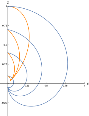
Figure 2: Single-qubit geodesic curves in the $xz$-plane of the Bloch ball starting and ending at polar coordinates $(r_{1},0)$ and $(r_{2},\theta_{12})$, respectively. The curves have the form $r(\theta)(\sin\theta,0,\cos\theta)$ with $r(\theta)$ given by Eq. (18). We have chosen $r_{1}=r(0)=0.1,0.4,0.7,1$ and $r_{2}=r(\theta_{12})=0.05$. The angular position of the end-points are $\theta_{12}=\frac{\pi}{4}$ (orange curves) and $\theta_{12}=\pi$ (blue curves).

The length of the geodesics can be computed by inserting Eq. (18) into Eq. (16) and performing the integration. One finds

$$l_{\rm g}=\frac{1}{2}\sqrt{\theta_{12}^{2}+\left(\arcsin r_{2}-\arcsin r_{1}\right)^{2}}.$$ (19)

We note that the geodesics for $r_{2}=r_{1}$ are circle arcs of length $\theta_{12}/2$, which is half the geodesic distance on $\mathcal{S}^{2}$. For pure ($r_{1}=r_{2}=1$) states, this is consistent with the Fubini-Study distance for single qubits anandan90 . $l_{g}$ measures the distance between non-degenerate qubit states.

III.4 Thermal magnetic systems

We illustrate the metric in Eq. (7) by considering the response of a magnetic system in a thermal state to changes in temperature $T$ and in an applied magnetic field $b$. This is modeled by the Hamiltonian $H(b)=H_{0}+bS_{z}$, $H_{0}$ being a generic Hamiltonian describing interactions between a collection of spins and $S_{z}$ is the total spin of the system. Let $\{|m(b)\rangle\}$ and $\{\varepsilon_{m}(b)\}$ be eigenstates and eigenvalues, respectively, of $H(b)$. The thermal state takes the form $\rho=e^{-\beta H(b)}/Z$ with $Z={\rm Tr}\left(e^{-\beta H(b)}\right)$ the partition function and $\beta$ the inverse temperature. The following analysis shows that the metric can be related to thermodynamic quantities.

Let us first consider changes in temperature. One finds

$$ds^{2} = \frac{C_{V}}{4\beta^{2}}d\beta^{2},$$ (20)

where $C_{V}$ is specific heat for a Boltzmann distribution, being related to the energy fluctuations according to $C_{V}=\beta^{2}\left(\langle\varepsilon^{2}\rangle-\langle\varepsilon\rangle^{2}\right)$. Here and in the following, $\langle\cdot\rangle$ is the thermodynamic average obtained by means of the Boltzmann factors $p_{m}=e^{-\beta\varepsilon_{m}(b)}/Z$. For changes in the applied magnetic field, we find

$$ds^{2} = \left(\frac{\beta\chi_{M}}{4}+\sum_{m}p_{m}\chi_{F,m}\right)db^{2}$$ (21)

with the magnetic susceptibility $\chi_{M}=\beta\left[\left\langle\left(\partial\varepsilon/\partial b\right)^{2}\right\rangle-\left\langle\partial\varepsilon/\partial b\right\rangle^{2}\right]$ and the fidelity susceptibility you07

$$\chi_{F,m}(b)=\sum_{m^{\prime}\neq m}\frac{\left|\langle m^{\prime}|S_{z}|m\rangle\right|^{2}}{(\varepsilon_{m}-\varepsilon_{m^{\prime}})^{2}}$$ (22)

of state $m$.

IV Relation to Bures’ metric

Before concluding, we justify our distance concept by demonstrating that the Bures metric hubner92 ; uhlmann92 can be obtained if we extend Eq. (3) to arbitrary decompositions of $\rho(t)$. We use that the set

$$\mathcal{A}(t) = \left\{\sum_{l}\sqrt{p_{l}(t)}|n_{l}(t)\rangle\mathbb{V}_{lk}(t)\right\}$$ (23)

of sub-normalized vectors is a decomposition of $\rho(t)$ for any unitary $N^{\prime}\times N^{\prime}$ matrix $\mathbb{V}$ with $N^{\prime}-N$ zero vectors added schrodinger36 ; hughston93 . If $\mathcal{B}(t)$ is replaced by $\mathcal{A}(t)$ in Eq. (3), we find the distance

$$\tilde{d}^{2}(t,t+dt)=2-2{\rm Re}{\rm Tr}\left[\mathbb{M}_{t}(dt)\mathbb{V}(t+dt)\mathbb{V}^{\dagger}(t)\right],$$ (24)

where $\left[\mathbb{M}_{t}(dt)\right]_{kl}=\sqrt{p_{k}(t)p_{l}(t+dt)}\langle n_{k}(t)|n_{l}(t+dt)\rangle$ is the overlap matrix. By means of the polar decomposition $\mathbb{M}_{t}(dt)=\big{|}\mathbb{M}_{t}(dt)\big{|}\mathbb{U}_{t}(dt)$, we find the line element

$$d\tilde{s}^{2}=\tilde{d}_{\min}^{2}(t,t+dt)=2-2{\rm Tr}\big{|}\mathbb{M}_{t}(dt)\big{|},$$ (25)

by choosing $\mathbb{V}$ such that $\mathbb{U}_{t}(dt)\mathbb{V}(t+dt)\mathbb{V}^{\dagger}(t)=\mathbb{I}$. One may use the spectral form of $\rho(t)$ and $\rho(t+dt)$ and the orthonormality of $\left\{|n_{k}(t)\rangle\right\}$ to obtain

$$\sqrt{\rho(t)}\rho(t+dt)\sqrt{\rho(t)}$$ (26)

$$= \left(\sum_{k,k^{\prime}}|n_{k}(t)\rangle\left|\mathbb{M}_{t}(dt)\right|_{kk^{\prime}}\langle n_{k^{\prime}}(t)|\right)$$

$$\times\left(\sum_{l^{\prime},l}|n_{l^{\prime}}(t)\rangle\left|\mathbb{M}_{t}(dt)\right|_{l^{\prime}l}\langle n_{l}(t)|\right),$$

from which we conclude

$$\sqrt{\sqrt{\rho(t)}\rho(t+dt)\sqrt{\rho(t)}}$$ (27)

$$= \sum_{k,l}|n_{k}(t)\rangle\left|\mathbb{M}_{t}(dt)\right|_{kl}\langle n_{l}(t)|.$$

By taking the trace, we see that Eq. (25) can be expressed as

$$d\tilde{s}^{2}=2-2{\rm Tr}\sqrt{\sqrt{\rho(t)}\rho(t+dt)\sqrt{\rho(t)}},$$ (28)

which is precisely the Bures line element hubner92 ; uhlmann92 .

V Conclusions

The concept of metric associated with the spectral decomposition of mixed quantum states is delineated and its physical significance discussed. This completes the theory of mixed state GP proposed in Ref. sjoqvist00 , in the same way as the Fubini-Study and the Bures metric complete the theory of pure state geometric phase and Uhlmann holonomy, respectively. The relation to energy-time uncertainty and thermodynamics found above, suggests that the proposed metric can be expected to find applications in the problem of finding time-optimal evolutions of mixed quantum states as well as in the study of phase transitions in many-body quantum systems at non-zero temperatures.

References

- (1) W. K. Wootters, Statistical distance and Hilbert space, Phys. Rev. D 23, 357 (1981).
- (2) S. L. Braunstein and C. M. Caves, Statistical distance and the geometry of quantum states, Phys. Rev. Lett. 72, 3439 (1994).
- (3) A. Shimony, Degree of Entanglement, Ann. N.Y. Acad. Sci. 755, 675 (1995).
- (4) V. Vedral, M. B. Plenio, M. A. Rippin, and P. L. Knight, Quantifying Entanglement, Phys. Rev. Lett. 78, 2275 (1997).
- (5) T.-C. Wei and P. M. Goldbart, Geometric measure of entanglement and applications to bipartite and multipartite quantum states, Phys. Rev. A 68, 042307 (2003).
- (6) L. C. Venuti and P. Zanardi, Quantum Critical Scaling of the Geometric Tensors, Phys. Rev. Lett. 99, 095701 (2007).
- (7) W.-L. You, Y.-W. Li, S.-J. Gu, Fidelity, dynamic structure factor, and susceptibility in critical phenomena, Phys. Rev. E 76, 022101 (2007).
- (8) A. Carlini, A. Hosoya, T. Koike, and Y. Okudaira, Time-Optimal Quantum Evolution, Phys. Rev. Lett. 96, 060503 (2006).
- (9) N. Margolus, L. B. Levitin, The maximum speed of dynamical evolution, Physica D 120, 188 (1998).
- (10) S. Deffner and E. Lutz, Quantum Speed Limit for Non-Markovian Dynamics, Phys. Rev. Lett. 111, 010402 (2013).
- (11) D. Mondal and A. K. Pati, Quantum speed limit for mixed states using an experimentally realizable metric, Phys. Lett. A 380, 1395 (2016).
- (12) Y. Aharonov and J. Anandan, Phase change during a cyclic quantum evolution, Phys. Rev. Lett. 58, 1593 (1987).
- (13) J. P. Provost and G. Vallee, Riemannian structure on manifolds of quantum states, Commun. Math. Phys. 76, 289 (1980).
- (14) J. Anandan and Y. Aharonov, Geometry of Quantum Evolution, Phys. Rev. Lett. 65, 1697 (1990).
- (15) A. Uhlmann, Parallel transport and quantum holonomy along density operators, Rep. Math. Phys. 24, 229 (1986).
- (16) M. Hübner, Explicit computation of the Bures distance for density matrices, Phys. Lett. A 163, 239 (1992).
- (17) E. Sjöqvist, A. K. Pati, A. Ekert, J. S. Anandan, M. Ericsson, D. K. L. Oi, and V. Vedral, Geometric Phases for Mixed States in Interferometry, Phys. Rev. Lett. 85, 2845 (2000).
- (18) D. M. Tong, E. Sjöqvist, L. C. Kwek, and C. H. Oh, Kinematic Approach to the Mixed State Geometric Phase in Nonunitary Evolution, Phys. Rev. Lett. 93, 080405 (2004).
- (19) J. Du, P. Zou, M. Shi, L. C. Kwek, J.-W. Pan, C. H. Oh, A. Ekert, D. K. L. Oi, and M. Ericsson, Observation of Geometric Phases for Mixed States using NMR Interferometry, Phys. Rev. Lett. 91, 100403 (2003);
- (20) M. Ericsson, D. Achilles, J. T. Barreiro, D. Branning, N. A. Peters, and P. G. Kwiat, Measurement of Geometric Phase for Mixed States Using Single Photon Interferometry, Phys. Rev. Lett. 94, 050401 (2005).
- (21) J. Klepp, S. Sponar, S. Filipp, M. Lettner, G. Badurek, and Y. Hasegawa, Observation of Nonadditive Mixed-State Phases with Polarized Neutrons, Phys. Rev. Lett. 101, 150404 (2008).
- (22) O. Andersson, Holonomy in Quantum Information Geometry, arxiv:1910.08140.
- (23) A. Uhlmann, An energy dispersion estimate, Phys. Lett. A 161, 329 (1992).
- (24) The absence of the factor in the angular part of the line element implies that the metric is singular at the origin of the Bloch ball, corresponding to a degenerate qubit state. This is an illustration of the general fact that the metric is undefined for degenerate density operators.
- (25) E. Schrödinger, Probability relations between separated systems, Proc. Camb. Phil. Soc. 32, 446 (1936).
- (26) L. P. Hughston, R. Jozsa, and W. K. Wootters, A complete classification of quantum ensembles having a given density matrix, Phys. Lett. A 183, 14 (1993).
- (27) I. Bengtsson and K. Życzkowski, Geometry of quantum states (Cambridge University Press, Cambridge, 2006).