Instabilities of Time-averaged Configurations in Thermal Glasses

Abstract

In amorphous solids at finite temperatures the particles follow chaotic trajectories which, at temperatures sufficiently lower than the glass transition, are trapped in “cages”. Averaging their positions for times shorter than the diffusion time, one can define a time-averaged configuration. Under strain or stress, these average configurations undergo sharp plastic instabilities. In athermal glasses the understanding of plastic instabilities is furnished by the Hessian matrix, its eigenvalues and eigenfunctions. Here we propose an uplifting of Hessian methods to thermal glasses, with the aim of understanding the plastic responses in the time averaged configuration. We discuss a number of potential definitions of Hessians and identify which of these can provide eigenvalues and eigenfunctions which can explain and predict the instabilities of the time-averaged configurations. The conclusion is that the non-affine changes in the average configurations during an instability is accurately predicted by the eigenfunctions of the low-lying eigenvalues of the chosen Hessian.

I Introduction

The theory of the micro-mechanics of plasticity and material failure of amorphous solids at finite temperatures lags behind the understanding of the athermal counterpart. At $T=0$ an amorphous solids in mechanical equilibrium can be usefully characterized by the eigenfunctions and eigenvalues of the Hessian matrix. In a system with $N$ particles in a volume $V$ in $d$ dimensions and a Hamiltonian $U({\bm{r}}_{1},{\bm{r}}_{2}\dots,{\bm{r}}_{N})$, where the particles’ coordinates are $\{{\bm{r}}_{i}\}_{i=1}^{N}$, the Hessian matrix is defined as

$$H_{ij}\equiv\frac{\partial^{2}U({\bm{r}}_{1},{\bm{r}}_{2}\dots,{\bm{r}}_{N})}{\partial{\bm{r}}_{i}\partial{\bm{r}}_{j}}\ .$$ (1)

Being a symmetric real matrix the eigenvalues $\{\lambda_{i}\}_{i=1}^{dN}$ of ${\bm{H}}$ are real and semi-positive as long as the system is mechanically stable. The normal modes of the system have frequencies $\omega_{i}\equiv\sqrt{\lambda_{i}}$ from which the density of states can be calculated. Mechanical instabilities are associated with non-zero eigenvalues going to zero, and the associated eigenfunction predicts the non-affine material response during the instability Lemaître and Maloney (2006); Karmakar et al. (2010).

Once the system gains thermal energy at temperature $T$, it is never in mechanical equilibrium since the particles constantly dance around a mean position. Thus a temporal Hessian calculated at any given time will exhibit negative eigenvalues and will be less useful in predicting instabilities or providing structural information Palyulin et al. (2018). Nevertheless, at temperatures low enough compared to the glass transition temperature $T_{g}$, the particles are stuck for sufficiently long times in cages, allowing us to compute their average positions. It is therefore interesting and relevant to attempt to characterize the average configurations and their instabilities using a modified Hessian $\hat{{\bm{H}}}$ which is adapted for the thermal conditions. In Sect. II we discuss a number of candidates, requiring a minimal condition that as long as the average positions are stationary and stable, the eigenvalues of $\hat{{\bm{H}}}$ were semipositive, in contradistinction with the instantaneous Hessian Eq. (1). Having a number of candidate, we test their efficacy in a standard model of a glass former which is described in Sect. III. In Sect. IV we motivate the selection of one of the candidate Hessian which appears to provide an excellent characterization of the plastic events in the average configurations. In fact the non-affine displacement of the average particle positions during a plastic event can be understood from the knowledge of the eigenvalues and eigenfunctions of $\hat{{\bm{H}}}$ just before the event takes place.

Possibly one of the interesting conclusions of this study is that providing a typical glass forming system with temperature is not like increasing the level of allowed motion on top of the athermal energy landscape. The dynamics which temperature allows results in momentum transfers that are interpreted as effective forces between the particles that are very different from the bare forces Brito and Wyart (2006); Gendelman et al. (2016); Parisi et al. (2018, 2019). Thus even when the bare forces are binary, the dressed forces gain ternary, quaternary and higher order components due to multiple interactions between particles. If one thinks of these forces as derivable from an effective Hessian as discuss below, it becomes obvious that the resulting “energy landscape” becomes quite different from the athermal counterpart, and explicitly temperature dependent. This important point is emphasized below in the conclusion section.

II Candidate Hessians

The first derivation of a microscopic theory of the response of the materials to external mechanical strains was developed by Born (see, e.g., Born and Huang (1998); Maradudin et al. (1963)) for athermal systems. Further developments of the microscopic theory of elasticity at finite temperatures using statistical mechanics were offered in Ref. Squire and Hoover (1969). The result is that thermal corrections to the Born theory include fluctuation terms, the magnitude of which are significant at high temperatures, vanishing at zero temperature in the case of perfect crystals. A generalization of this approach to arbitrary systems in the solid state was developed in Lutsko (1989). The limit of zero temperatures in this approach indicates the existence of non-vanishing fluctuation contributions in systems that are more complex than the perfect crystal. Considering systems at zero temperature has an obvious advantage: it is possible to study the response of a single configuration which is an “inherent state” Stillinger and Weber (1984). This allows us to use a purely mechanical approach Lemaître and Maloney (2006); Maloney and Lemaître (2006); Karmakar et al. (2010); Hentschel et al. (2011); Dasgupta et al. (2012a, b) which is very useful in studying mechanical properties of amorphous solids. The Hessian matrix, whose eigenvalues are semi-positive at $T=0$, provides important information, leading to an athermal theory that provides good understanding of the density of states, of plastic events, and of the failure mechanisms of amorphous solids.

In order to lift the methods that were so useful at $T=0$ to finite temperatures one needs to recognize that although the particle positions in a thermal systems are indeed not stationary, in glasses with large relaxation times one can determine the averaged positions much before the onset of diffusion or the glass relaxation to thermodynamic equilibrium. The averaged positions are obviously stationary, and can be used to determine the renormalized force laws that hold these average positions stable Brito and Wyart (2006); Gendelman et al. (2016); Parisi et al. (2018, 2019). It was recognized that the renormalized forces are very different from the bare forces. For example even if the bare forces are binary, the renormalized forces are not; generically they contain ternary, quaternary and higher order contribution Gendelman et al. (2016); Parisi et al. (2018, 2019). The effective potential from which such renormalized forces can be derived is in general not known. We thus need to proceed with care in searching the “correct” effective Hessian that may provide useful predictions for the plastic instabilities of the average configuration of a thermal glass under external strains and stresses. In this section we demonstrate possible definitions of an effective Hessian at finite temperatures with the aim of rationalizing instabilities in the average configurations.

Consider a glassy system composed of $N$ particles with time dependent positions $\{{\bm{r}}_{i}(t)\}_{i=1}^{N}$ which is endowed with a Hamiltonian $U\left({\bm{r}}_{1}(t),\cdots,{\bm{r}}_{N}(t)\right)$. Assume that the system is in temperature $T$ which is sufficiently low so that the glassy relaxation time (or the effective diffusion time) $\tau_{G}$ is long enough, so that one can compute the time averaged positions ${\bm{R}}_{i}$:

$${\bm{R}}_{i}\equiv\frac{1}{\tau}\int_{0}^{\tau}dt~{}{\bm{r}}_{i}(t)\ ,$$ (2)

where $\tau\ll\tau_{G}$. By definition the positions ${\bm{R}}_{i}$ are time independent and the configuration $\{{\bm{R}}_{i}\}_{i=1}^{N}$ is stable, at least for the time interval $[0,\tau_{G}]$. In addition to the mean positions we will employ below also the covariance matrix ${\bm{\Sigma}}$ defined as

$${\bm{\Sigma}}_{ij}\equiv\frac{1}{\tau}\int_{0}^{\tau}dt\left({\bm{r}}_{i}(t)-{\bm{R}}_{i}\right)\left({\bm{r}}_{j}(t)-{\bm{R}}_{j}\right)\ .$$ (3)

We can then define three different effective Hessians as follows:

II.1 Hessian computed at the average positions.

To emphasize the fact that the bare Hessian which is computed from the bare potential (which is fully sufficient at zero temperature) is not providing useful information at finite temperatures, we consider the first possible candidate Hessian, denoted as ${\bm{H}}^{(1)}$. Here derivatives of the bare potential are computed at the average positions:

$${\bm{H}}^{(1)}_{ij}=\frac{\partial U({\bm{r}}_{1}\cdots{\bm{r}}_{N})}{\partial{\bm{r}}_{i}\partial{\bm{r}}_{j}}\Big{|}_{{\bm{r}}_{i}={\bm{R}}_{i},{\bm{r}}_{j}={\bm{R}}_{j}}\ .$$ (4)

II.2 Hessian computed as the time average of the instantaneous Hessian

Following the success of computing the effective forces in thermal glasses as the time average of the instantaneous forces Gendelman et al. (2016); Parisi et al. (2018, 2019) one can try also to time average the instantaneous Hessian, denoting it ${\bm{H}}^{(2)}$:

$${\bm{H}}_{ij}^{(2)}\equiv\frac{1}{\tau}\int_{0}^{\tau}dt\frac{\partial^{2}U({\bm{r}}_{1}(t),{\bm{r}}_{2}(t)\dots,{\bm{r}}_{N}(t))}{\partial{\bm{r}}_{i}(t)\partial{\bm{r}}_{j}(t)}\ ,$$ (5)

where the integration time $\tau$ is large enough to achieve convergence and small enough for the cage structure to remain intact. One could hope that this candidate Hessian would be sensitive to the dynamics to be able to provide useful information.

II.3 Hessian computed from the inverse of the covariance matrix

The third candidate Hessian is the most tricky, since it is based on the notion of effective potential. As said above, in amorphous solids we can define the average positions ${\bm{R}}_{i}$ which are stationary in time, and can consider the effective forces $\hat{{\bm{F}}}$ that stabilize these positions. These forces are determined by the momentum transfer during the dynamics, but the momentum transferred between particles $i$ and $j$ can depend on intervening interaction between particles $i$ and $k$ (leading to ternary rather than binary effective interactions), or between particle $i$, $k$ and $\ell$, giving rise to quaternary effective interactions etc. While the bare force on the $i$th particle $-\partial U/\partial{\bm{r}}_{i}$ does not vanish at ${\bm{R}}_{i}$, we can think of an effective Hamiltonian $\hat{U}$ from which (in principle) the effective forces $\hat{{\bm{F}}}_{i}$ can be derived, and of course should satisfy the condition $-\partial\hat{U}/\partial{\bm{r}}_{i}=0$ when computed at ${\bm{R}}_{i}$.

Although we do not have an explicit solution for the effective potential $\hat{U}$, we can still Taylor expand it around the average positions ${\bm{R}}_{i}$:

$$\hat{U}(\{{\bm{r}}_{i}\})=\hat{U}(\{\bf R_{i}\})+\frac{1}{2}\tilde{{\bf u}}{\bf H}^{(3)}\large|_{\bf R}{\bf u}+\cdots,$$ (6)

where ${\bf u}=\{{\bm{r}}_{i}-{\bm{R}}_{i}\}$ is the set of particle displacements from the average. The candidate Hessian ${\bm{H}}^{(3)}$ is given by

$${\bm{H}}_{ij}^{(3)}=\frac{\partial^{2}\hat{U}(\{\bf r_{i}\})}{\partial{\bm{r}}_{i}\partial{\bm{r}}_{j}}\large|_{\bf R_{i},{\bm{R}}_{j}}\ .$$ (7)

Of course, at this point the definition is useless since we do not know the actual form of $\hat{U}({\bf r_{i}})$. But if we did we could also compute the average positions and the covariance matrix according to

$${\bm{R}}_{i}=\frac{\int{\bm{r}}_{i}e^{-\frac{\hat{U}(\{\bf r_{j}\})}{k_{B}T}}d\{\bf r_{j}\}}{\int e^{-\frac{\hat{U}(\{{\bm{r}}_{j}\})}{k_{B}T}}d\{\bf r_{j}\}}$$ (8)

$$\langle{\bm{r}}_{i}{\bm{r}}_{j}\rangle=\frac{\int{\bm{r}}_{i}{\bm{r}}_{j}e^{-\frac{\hat{U}(\{\bf r_{k}\})}{k_{B}T}}d\{\bf r_{k}\}}{\int e^{-\frac{\hat{U}(\{{\bm{r}}_{k}\})}{k_{B}T}}d\{\bf r_{k}\}}$$ (9)

Knowing the first and the second moments one can define the multivariate Gaussian distribution

$$f({{\bm{r}}})=C\exp\bigg{\{}-\frac{1}{2}\widetilde{({\bm{r}}-{\bm{R}})}{{\bm{\Sigma}}}^{-1}({\bm{r}}-{\bm{R}})\bigg{\}}\ .$$ (10)

Comparing Eq. (6) and Eq. (10) one identifies

$${\bf H}^{(3)}=k_{B}T{\bf\Sigma}^{-1}.$$ (11)

We should note at this point that the covariance matrix is positive semidefinite only, due to the existence of Goldstone modes, and Eq. (11) should be replaced by

$${\bf H}^{(3)}=k_{B}T{\bf\Sigma}^{+},$$ (12)

where ${\bf\Sigma}^{+}$ is the pseudo inverse of the covariance matrix. Of course, the effective Hessian given by Eq. (12) and the covariance matrix have the same set of eigenfunctions

$${\bf H}^{(3)}{\bf\Psi}_{i}=\lambda^{H}_{i}{\bf\Psi}_{i}$$ (13)

and their eigenvalues are related by

$$\lambda^{H}_{i}=\frac{k_{B}T}{\lambda_{i}^{\Sigma^{+}}}\ .$$ (14)

This approach was used to study the vibrational spectra of colloids and granular systems based on measurements using video and confocal microscopy (see e.g., Ghosh et al. (2010); Henkes et al. (2012)), and restoration of effective interaction potential using simulation methods Schindler and Maggs (2016). It should be stressed that this method appears to have been used only for unstrained systems. Below we will use this effective Hessian for shear strained systems before and after plastic responses.

In the next section we will use a standard model of glass formers to decide which of the candidate Hessians provides the information that we seek.

III Model

To make a choice between the three candidate Hessians we compute them together with their eigenvalues and eigenfunctions in a standard model of a glass former, i.e. a binary mixture of point particles interacting via inverse power-law potentials Perera and Harrowell (1999). 50% of the particles are “small” (type $A$) and the other 50% of the particles are “large” (type $B$). The interaction between particle $\alpha$ (being $A$ or $B$) and particle $\beta$ (being $A$ or $B$) are defined as

$$\phi_{\alpha\beta}(r)=\epsilon\Big{(}\frac{\sigma_{\alpha\beta}}{r}\Big{)}^{12}\ .$$ (15)

It is convenient to introduce reduced units, with $\sigma_{AA}=1$ being the units of length and $\epsilon=1$ the unit of energy (with Boltzmann’s constant being unity).

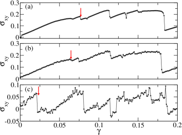
Figure 1: The stress averaged over 10,000 Monte Carlo sweeps vs. strain, for three different temperatures; panel a: $T=0.0001$; panel b: $T=0.01$; panel c: $T=0.1$. Arrows indicate the plastic events in the average configuration that are analyzed in detail below.

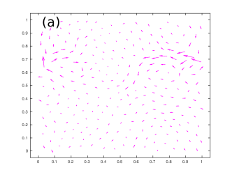
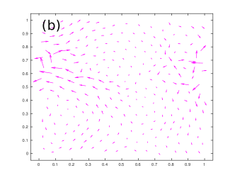
Figure 2: The non-affine displacement field for $T=0.0001$ (panel a), $T=0.01$ (panel b) and $T=0.1$ (panel c) measured for the time-averaged mean particle positions during the plastic drops indicated with arrows in Fig. 1.

III.1 Time-averaged configurations and their instabilities

Simulations were performed using a Monte Carlo method in an NVT ensemble of $N=256$ particle in a two dimensional box of size $L\times L$ with periodic boundary conditions. $L$ was chosen such that at any temperature the density $\rho=0.76$ Perera and Harrowell (1999). The acceptance rate was chosen to be $30\%$ at all temperatures. We first equilibrate a system at a temperature $T=3$ and then cool it down in steps of $\Delta T=10^{-3}$ to a target temperature $0<T\leq 0.1$, where the upper limit was chosen since in this system $T_{g}\approx 0.3$ Perera and Harrowell (1999). Once the system is equilibrated at the target temperature we begin to strain the system by simple shear in a quasi-static manner. Here “quasi-static” means that after every small step of strain we allow the system to equilibrate performing 10,000 Monte Carlo sweeps. After completing the last Monte-Carlo sweep a small affine increase in strain $\Delta\gamma$ is defined by the volume preserving transformation

$$x^{\prime}_{i} = x_{i}+\Delta\gamma y_{i}$$

$$y^{\prime}_{i} = y.$$ (16)

In thermal glasses every such affine step destroys the thermal equilibrium, causing a change in the average positions and the covariance matrix. To regain equilibrium one should allow a nonaffine relaxation to a new average particle positions and covariance matrix. In the quasi-static protocol we make sure that the average positions are stabilized. Computing the average stress is done in a subsequent run of $1,500,000$ sweeps, again controlling convergence. Typical time-averaged stress $\sigma_{xy}$ vs strain $\gamma$ for temperatures $T=0.001$, $T=0.01$ and $T=0.1$ are shown in Fig. 1.

We note that the time-averaged stress exhibits sharp drops even at $T/T_{g}\approx 0.33$, and these are easily distinguishable from temperature fluctuations that are averaged out in these plots. We refer to the drops in the time-averaged stress as plastic drops. Our aim here is to understand, and possibly predict, the non-affine change in the average positions of particles (average displacement) that occur during these plastic drops, using the Hessian and its eigen-properties before the drop takes place.

To prepare for comparisons with theory we consider the non-affine displacement fields that are obtained from the time averaged configurations before and after a sharp drop. These displacement fields are obtained by subtracting from the measured change in averaged configurations the last affine step Eq. (16) before the drop. We denote below the normalized non-affine displacement field as ${\bf{\cal N}}({\bm{r}})$. Examples of such fields are shown in Fig. 2 for $T=0.0001$ (panel a), $T=0.01$ (panel b) and $T=0.1$ (panel c). The displacement fields shown here are associated with the plastic drops that are indicated with an arrow in Fig. 1.

We note that the observable sharp plastic drops in the time-averaged stress can be accompanied by non-affine displacement in the average configurations that can be either system spanning or localized. In our simulation systems spanning events are more prevalent, presumably smaller localized drops are swamped by temperature fluctuations.

IV Which Hessian?

At this point we are ready to select which Hessian fits the bill and provides a useful theory for understanding the instabilities and the non-affine displacements in the average configurations. For the present model, and presumably quite generally, the first candidate ${\bm{H}}^{(1)}$ can be ruled out quite immediately since its calculation at the average points yields negative eigenvalues similarly to the instantaneous Hessian. We thus do not discuss it further.

The second candidate ${\bm{H}}^{(2)}$ computed as the time average of the bare Hessian provides a semi-positive spectrum at all the simulated temperatures, with 2 zero eigenvalues for the Goldstone modes. It therefore appears on the face of it to be a valid candidate. However, computing the eigenvalues of ${\bm{H}}^{(2)}$ at a series of increasing temperatures reveals that even in the equilibrium state with zero strain these eigenvalues increase as a function of temperature. We propose that this is highly unphysical. One expects the amorphous solid to become softer as temperature increases, with eigenvalues going to zero at the glass transition temperature. We have checked that this unphysical behavior persists for different model Hamiltonians, including the standard Lennard-Jones glass Kob and Andersen (1994). A second problem with ${\bm{H}}^{(2)}$ is that its lowest eigenvalue never appears to approach zero near a plastic instability. Its eigenfunctions did not show resemblance to the non-affine events that we care to describe.

In hindsight, this should not be surprising. The bare Hessian has information about the binary interactions only, and by time averaging it we do not input anywhere the pertinent information about higher order interactions. Not having this information makes the second candidate useless. We thus discard this candidate Hessian from our list.

The third candidate Hessian ${\bm{H}}^{(3)}$ appears to provide us with the best guide for understanding the plastic instabilities as we demonstrate in detail in the next section. But it also agrees with physical intuition, providing eigenvalues that reduce with increasing temperature, exhibiting a semi-positive spectrum with two Goldstone modes. We thus drop from this point onward the superscript (3) and denote the chosen candidate Hessian as $\hat{{\bm{H}}}$ to distinguish it from the bare Hessian ${\bm{H}}$.

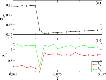
Figure 3: Panel a: the drop in the average stress expanded at $\gamma\approx 0.0755$. Panel b: the 2 lowest lying eigenvalues of the average Hessian $\hat{{\bm{H}}}$ as a function of strain in the expanded strain neighborhood of the sharp drop indicated with an arrow in Fig. 1. The temperature is $T=0.0001$.

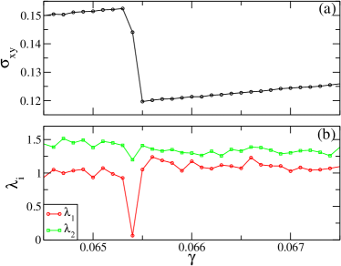
Figure 4: Panel a: the drop in the average stress expanded at $\gamma\approx 0.0653$. Panel b: the 2 lowest lying eigenvalues of the average Hessian $\hat{{\bm{H}}}$ as a function of strain in the expanded strain neighborhood of the sharp drop indicated with an arrow in Fig. 1. The temperature is $T=0.01$.

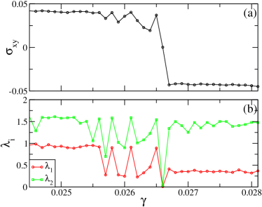
Figure 5: Panel a: the drop in the average stress expanded at $\gamma\approx 0.0265$. Panel b: the 2 lowest lying eigenvalues of the average Hessian $\hat{{\bm{H}}}$ as a function of strain in the expanded strain neighborhood of the sharp drop indicated with an arrow in Fig. 1. The temperature is $T=0.1$.

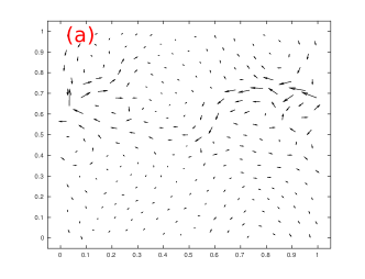
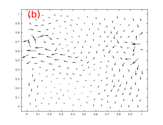
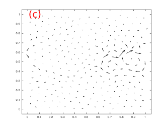
Figure 6: The eigenfunctions of $\hat{{\bm{H}}}$ associated with the lowest eigenvectors that tend to vanish at the plastic instability. Their visual resemblance to the actual non-affine displacement fields shown in Figs. 2 is clear, and is emphasized further in Fig. 7.

V Predicting non-affine time-averaged displacements

The most stringent test on the chosen Hessian is its ability to predict the nonaffine-displacement using its eigenfunctions and eigenvalues before the instability takes place. As said above, excluding Goldstone modes, the eigenvalues of $\hat{{\bm{H}}}$ are all real and positive as long as the system is stable. Moreover, they display a very weak dependence on the strain as long as the instability is not approached. An example of the strain-dependence stress and of the 2 lowest lying eigenvalues of $\hat{{\bm{H}}}$ are shown in Fig. 3-5 for all the three temperatures in Fig. 1. We see that there is a clear tendency for the lowest positive eigenvalue to vanish at strain values that correspond to the sharp stress drops.

At this point consider the eigenfunctions ${\bm{\Psi}}_{1}$ of $\hat{{\bm{H}}}$ which are associated with the lowest-lying eigenvalues $\lambda_{1}$ at the three temperatures discussed here. In Fig. 6 we show the three eigenfunctions associated with the lowest eigenvalue at each temperature, and these should be compared with the non-affine displacement fields in Fig. 2. It is obvious to the eye that the correspondence is quite striking. To emphasize this correspondence we shown in Fig. 7 the non-affine displacements superimposed on the eigenfunctions. A quantitative measure of the agreement (and the predictability of the non-affine displacement field form the eigenfunction) is obtained by normalizing the displacement field and computing the scalar product $a_{1}\equiv{\bf{\cal N}}({\bm{r}})\cdot{\bm{\Psi}}_{1}$ with the (orthonormal) eigenfunction. For the three temperatures discussed here we find the scalar product to be 0.981 for $T=0.0001$, 0.893 for $T=0.01$ and 0.992 for $T=0.1$. Obviously, the eigenfunction associated with the eigenvalue that goes to zero at the instability are able to predict the non-affine displacement field in the average position quite successfully. It is very interesting that this predictive capability exists even at $T=0.1$ which is about a third of $T_{g}$.

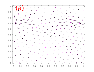
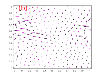
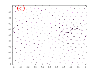
Figure 7: A comparison between the eigenfunctions and the actual non-affine displacement fields of the average configurations. Here we superimposed the non-affine displacement fields shown in Figs. 2 with the eigenfunctions shown in Fig. 6. Their visual resemblance is striking.

VI Summary and Conclusions

In this paper we examined the lifting of athermal Hessian methods to glasses at finite temperatures. The main idea is that at temperatures that are low enough one can determine a stationary average positions of all the involved particles. Such a configuration has a vanishing effective force on each particle, exactly as at $T=0$ in an inherent state. A well chosen Hessian matrix then should supply information about plastic instabilities that is as useful as the bare Hessian at $T=0$. A-priori it is not obvious how to define such a “well chosen” Hessian. We have examined in the present paper a number of candidates, and discovered that the effective Hessian that is found from inverting the covariance matrix is the most appropriate. It exhibits eigenvalue that decrease upon increasing temperatures, in agreement with the expectation that the glassy solid softens up upon heating. More importantly, the lowest eigenvalues of this Hessian tend to vanish at the strain values where the average stress suffers sharp drops indicating an important plastic rearrangement in the average positions of the particles. We discovered that the eigenfunctions associated with the lowest eigenvalue have almost full projection on the nonaffine displacement field, providing us with a useful predictability of the non-affine plastic event.

Having in mind the usefulness of the Hessian methods at athermal conditions, we trust that the present results should have further implication on the study and understanding of the mechanical properties of thermal glasses.