Determining two coefficients in diffuse optical tomography
with incomplete and noisy Cauchy data

Tran Nhan Tam Quyen

Abstract In this paper we investigate the non-linear and ill-posed inverse problem of simultaneously identifying the conductivity and the reaction in diffuse optical tomography with noisy measurement data available on an accessible part of the boundary. We propose an energy functional method and the total variational regularization combining with the quadratic stabilizing term to formulate the identification problem to a PDEs constrained optimization problem. We show the stability of the proposed regularization method and the convergence of the finite element regularized solutions to the identification in the $L^{s}$-norm for all $s\in[0,\infty)$ and in the sense of the Bregman distance with respect to the total variation semi-norm. To illustrate the theoretical results, a numerical case study is presented which supports our analytical findings.

Key words and phrases Diffusion-based optical tomography, diffuse optical tomography (DOT), electrical impedance tomography (EIT), simultaneous identification, finite element method, conductivity/diffusion coefficient, reaction/absorption coefficient.

AMS Subject Classifications 35R25; 47A52; 35R30; 65J20; 65J22.

1 Introduction

Electrical impedance tomography is a noninvasive type of medical imaging, where the tomographic image of the electrical conductivity, permittivity, and impedance of a body part is desired to infer from surface electrode measurements. This problem attracted a great deal of attention from many applied scientists in the last decades. For surveys on the subject, we refer the reader to, e.g., [13, 16, 27, 29, 30, 63, 76] and the references given there.

Mathematically, assume that the electric potential or voltage $u$ in the body $\Omega$ is governed by the equation

$$\nabla\cdot\big{(}q\nabla u\big{)}=0\quad\mbox{in}\quad\Omega\subset\mathbb{R}^{d},\quad d\geq 2$$

with a free source. Here $q=q(x),\enskip x\in\Omega$ is the electrical conductivity which must be identified from some measurements of the state $u$ on the boundary $\partial\Omega$ of the body $\Omega$. In an ideal situation we know all the voltages $u_{|\partial\Omega}:=g\in H^{1/2}(\partial\Omega)$ and the outward pointing normal component of the current densities $\Lambda^{\partial\Omega}_{q}g:={q\frac{\partial u}{\partial\vec{n}}}_{|\partial\Omega}:=j\in H^{-1/2}(\partial\Omega)$ as well, i.e. the knowledge of the Dirichlet-to-Neumann map

$$\Lambda^{\partial\Omega}_{q}:H^{1/2}(\partial\Omega)\rightarrow H^{-1/2}(\partial\Omega)$$

is described, where $\vec{n}$ is the unit outward normal on $\partial\Omega$. This is the continuum model which is commonly used in mathematical researches on the question of the solution uniqueness

$$p,q\in\mathcal{C}\subset L^{\infty}(\Omega)\quad\mbox{with}\quad\Lambda^{\partial\Omega}_{p}=\Lambda^{\partial\Omega}_{q}\quad\Rightarrow\quad p=q.$$

In dimensions three and higher the uniqueness result has been investigated by Sylvester and Uhlmann [74], Päivärinta el al. [65], and Brown and Torres [17], depending on the smoothness of considered conductivities. Meanwhile for the two dimensional setting it can be found in Nachman [64], Brown and Uhlmann [18], and Astala and Päivärinta [6].

In practice we however do not know all the voltage and current density $(g,j)$ on the boundary $\partial\Omega$, we measure them at some discrete electrodes posed on a relatively open subset $\Gamma$ of the boundary only. An interpolation process is then required to derive the measured voltage and current density $(g_{\delta},j_{\delta})$ on $\Gamma$, where $\delta>0$ refers to the error level of the interpolation process and/or the measurements. The identification is now to reconstruct the electrical conductivity $q$ distributed inside the body $\Omega$ from boundary measurements of the voltage and current density, i.e. from the pair $(g_{\delta},j_{\delta})$. This problem is known to be non-linear and severely ill-posed, due to the lack of data. To have an overview on numerical reconstruction for this identification problem one can examine, e.g., [55, 56, 61].

In the present paper we investigate the problem of simultaneously identifying the conductivity (or diffusion) and the reaction (or absorption), subjecting several sets of measurement data on an accessible part of the boundary are available. The identification problem is a theme of diffuse optical tomography — a category of applied sciences, e.g., neuroscience, medicine, wound monitoring and cancer detection. The interested reader may consult an incomplete list of references [3, 5, 12, 21, 31, 35, 44, 46, 49, 53, 62, 67, 69] for detailed discussions on this issue. In fact, assume $\Omega$ is an open, bounded and connected subset of $\mathbb{R}^{d},~{}d\geq 2$ with Lipschitz boundary $\partial\Omega$ and $\Gamma\subset\partial\Omega$ is a $(d-1)$-dimensional measurable surface. We consider the elliptic equation

$$-\nabla\cdot\big{(}q\nabla u\big{)}+au =f\quad\mbox{~{}in}\quad\Omega,$$ (1.1)

$$q\nabla u\cdot\vec{n}+\sigma u =j^{\dagger}\quad\mbox{on}\quad\Gamma,$$ (1.2)

$$q\nabla u\cdot\vec{n}+\sigma u =j_{0}\quad\mbox{on}\quad\partial\Omega\setminus\Gamma,$$ (1.3)

$$u =g^{\dagger}\quad\mbox{on}\quad\Gamma,$$ (1.4)

where the source term $f\in H^{-1}(\Omega):={H^{1}(\Omega)}^{*}$, the Neumann boundary condition $j_{0}\in H^{-1/2}(\partial\Omega\setminus\Gamma):={\left(H^{1/2}(\partial\Omega\setminus\Gamma)\right)}^{*}$ (see §2.1 for the definition of Sobolev spaces on surfaces), and the Robin coefficient $\sigma$ are assumed to be known with $\sigma\in L^{\infty}(\partial\Omega)$ and $\sigma(x)\geq 0$ a.e. on $\partial\Omega$. The identification problem is to seek the pair $(q,a)$ in the aforementioned equation (1.1) – (1.4) assuming the full knowledge of all Cauchy data on $\Gamma$

$$\mathcal{C}:=\left\{\big{(}{q\nabla u\cdot\vec{n}}_{|\Gamma}+\sigma u_{|\Gamma},u_{|\Gamma}\big{)}=:(j,g)\in H^{-1/2}(\Gamma)\times H^{1/2}(\Gamma)\right\}$$

is given. Arridge and Lionheart showed in [4] the non-uniqueness of this identification problem for globally smooth identified coefficients. Nevertheless, Harrach in [42] (see also [43]) proved that the identification problem is uniquely solvable in the class of piecewise constant functions.

Our aim in this work is to reconstruct the pair $(q,a)\in Q\times A$ from several sets of measurement data $\big{(}j^{i}_{\delta},g^{i}_{\delta}\big{)}_{i=1,\cdots,I}\subset H^{-1/2}(\Gamma)\times H^{1/2}(\Gamma)$ of the exact data $\big{(}j^{\dagger},g^{\dagger}\big{)}$ satisfying the noisy model

$$\frac{1}{I}\left(\big{\|}j^{i}_{\delta}-j^{\dagger}\big{\|}_{H^{-1/2}(\Gamma)}+\big{\|}g^{i}_{\delta}-g^{\dagger}\big{\|}_{H^{1/2}(\Gamma)}\right)\leq\delta$$ (1.5)

with $\delta>0$ standing for the error level of the observations. Here the admissible sets are assumed to be constrained of the general type

$$Q:=\{q\in L^{\infty}(\Omega)~{}|~{}\underline{q}\leq q(x)\leq\overline{q}\enskip\mbox{a.e. in}\enskip\Omega\}$$ (1.6)

and

$$A:=\{a\in L^{\infty}(\Omega)~{}|~{}\underline{a}\leq a(x)\leq\overline{a}\enskip\mbox{a.e. in}\enskip\Omega\},$$ (1.7)

where the constants $\underline{q},~{}\overline{q},~{}\underline{a},~{}\overline{a}$ are given with $0<\underline{q}\leq\overline{q}$ and $0<\underline{a}\leq\overline{a}$. Furthermore, for simplicity of exposition, hereafter we assume that $I=1$, i.e. only one Neumann-Dirichlet pair $(j_{\delta},g_{\delta})$ available. We also discuss the multiple measurement in Section 6.

With the pair $(j_{\delta},g_{\delta})$ at hand we examine the Neumann boundary value problem

$$-\nabla\cdot\big{(}q\nabla u\big{)}+au=f\quad\mbox{~{}in}\quad\Omega,\quad q\nabla u\cdot\vec{n}+\sigma u=j_{\delta}\quad\mbox{on}\quad\Gamma,\quad q\nabla u\cdot\vec{n}+\sigma u=j_{0}\quad\mbox{on}\quad\partial\Omega\setminus\Gamma$$ (1.8)

as well as the mixed boundary value problem

$$-\nabla\cdot\big{(}q\nabla v\big{)}+av=f\quad\mbox{~{}in}\quad\Omega,\quad v=g_{\delta}\quad\mbox{on}\quad\Gamma,\quad q\nabla v\cdot\vec{n}+\sigma v=j_{0}\quad\mbox{on}\quad\partial\Omega\setminus\Gamma$$ (1.9)

whose weak solutions are denoted by $N_{j_{\delta}}(q,a)$ and $M_{g_{\delta}}(q,a)$, respectively. Based on the variational approach of Kohn and Vogelius in [58, 59, 60], we propose the non-negative misfit energy functional

$$J_{\delta}(q,a) :=\int_{\Omega}q\left|\nabla\big{(}N_{j_{\delta}}(q,a)-M_{g_{\delta}}(q,a)\big{)}\right|^{2}dx+\int_{\Omega}a\big{(}N_{j_{\delta}}(q,a)-M_{g_{\delta}}(q,a)\big{)}^{2}dx$$

$$~{}\quad+\int_{\partial\Omega}\sigma\big{(}N_{j_{\delta}}(q,a)-M_{g_{\delta}}(q,a)\big{)}^{2}ds$$

for the identification problem and consider its minimizers over $Q\times A$ as reconstructions. However, since the identification problem is ill-posed, we make use a regularization method to seek stable solutions. Furthermore, for interests in estimating piecewise constant coefficients we therefore utilize total variation regularization combining with the quadratic stabilizing term, i.e. we consider the minimization problem

$$\min_{(q,a)\in Q_{ad}\times A_{ad}}\Upsilon_{\delta,\rho}(q,a):=J_{\delta}(q,a)+\rho R(q,a),$$

with

$$R(q,a) :=\int_{\Omega}|\nabla q|+\int_{\Omega}|\nabla a|+\frac{1}{2}\|q\|^{2}_{L^{2}(\Omega)}+\frac{1}{2}\|a\|^{2}_{L^{2}(\Omega)}$$

and

$$Q_{ad}:=Q\cap BV(\Omega)\enskip\mbox{and}\enskip A_{ad}:=A\cap BV(\Omega),$$

where $BV(\Omega)$ is the space of all functions of bounded total variation with the semi-norm $\int_{\Omega}|\nabla(\cdot)|$ and the norm $\int_{\Omega}|\nabla(\cdot)|+\|\cdot\|_{L^{1}(\Omega)}$ (cf. §2.2), and $\rho>0$ is the regularization parameter. Total variation regularization originally introduced in image denoising [72]. Somewhat later, it has been used to treat several ill-posed and inverse problems over the last decades, where the possibility of discontinuity in their solutions is interested in particular (cf. [20]). We would like to mention that for coefficient identification problems in partial differential equations with smooth enough identified objects one may employ the regularization of Sobolev norms (see, e.g., [1, 28, 51, 57]). In the present paper we adopt the stabilized method of total variation combining with quadratic term first introduced in [24] for linear inverse problems to treat the non-linear identification problem with possibly discontinuous sought coefficients.

Let $V^{h}_{1}$ be the finite dimensional space of piecewise linear, continuous finite elements, and $N^{h}_{j_{\delta}}(q,a)$ and $M^{h}_{g_{\delta}}(q,a)$ be respectively the finite element approximations of $N_{j_{\delta}}(q,a)$ and $M_{g_{\delta}}(q,a)$ in $V^{h}_{1}$, where $h>0$ is the mesh size of the triangulation. We then approximate the problem $\left(\mathcal{P}_{\delta,\rho}\right)$ by the discrete one

$$\min_{(q,a)\in Q^{h}_{ad}\times A^{h}_{ad}}\Upsilon^{h}_{\delta,\rho}(q,a):=J^{h}_{\delta}(q,a)+\rho R(q,a),$$

where

$$J^{h}_{\delta}(q,a) :=\int_{\Omega}q\left|\nabla\big{(}N^{h}_{j_{\delta}}(q,a)-M^{h}_{g_{\delta}}(q,a)\big{)}\right|^{2}dx+\int_{\Omega}a\big{(}N^{h}_{j_{\delta}}(q,a)-M^{h}_{g_{\delta}}(q,a)\big{)}^{2}dx$$

$$~{}\quad+\int_{\partial\Omega}\sigma\big{(}N^{h}_{j_{\delta}}(q,a)-M^{h}_{g_{\delta}}(q,a)\big{)}^{2}ds$$

and

$$Q^{h}_{ad}:=Q\cap V^{h}_{1}\subset Q\cap BV(\Omega)\enskip\mbox{and}\enskip A^{h}_{ad}:=A\cap V^{h}_{1}\subset A\cap BV(\Omega).$$

As the identification problem is non-linear and severely ill-posed, the stable analysis and convergence result of finite dimensional regularized solutions to the identification are crucial.

Let the regularization parameter $\rho$ and the observation data $(j_{\delta},g_{\delta})$ be fixed and $\big{(}q^{h_{n}}_{\delta,\rho},a^{h_{n}}_{\delta,\rho}\big{)}$ denotes an arbitrary minimizer of $\big{(}\mathcal{P}^{h_{n}}_{\delta,\rho}\big{)}$ for each $n\in\mathbb{N}$, where $h_{n}\to 0$ as $n\to\infty$. We then show that the sequence $\big{(}q^{h_{n}}_{\delta,\rho},a^{h_{n}}_{\delta,\rho}\big{)}$ has a subsequence converging to an element $\big{(}q_{\delta,\rho},a_{\delta,\rho}\big{)}\in Q_{ad}\times A_{ad}$ in the $L^{s}(\Omega)^{2}$-norm for all $s\in[1,\infty)$ with $\big{(}q_{\delta,\rho},a_{\delta,\rho}\big{)}$ a solution of $\big{(}\mathcal{P}_{\delta,\rho}\big{)}$.

Furthermore, let $\left(h_{n}\right)$ and $\left(\delta_{n}\right)$ be any positive sequences converging to zero together with $\rho_{n}=\rho_{n}(h_{n},\delta_{n})$ being suitably chosen. Assume that $\big{(}j_{\delta_{n}},g_{\delta_{n}}\big{)}$ is a sequence satisfying

$$\big{\|}j_{\delta_{n}}-j^{\dagger}\big{\|}_{H^{-1/2}(\Gamma)}+\big{\|}g_{\delta_{n}}-g^{\dagger}\big{\|}_{H^{1/2}(\Gamma)}\leq\delta_{n}$$

and that $\big{(}q^{h_{n}}_{\delta_{n},\rho_{n}},a^{h_{n}}_{\delta_{n},\rho_{n}}\big{)}$ is an arbitrary minimizer to $\big{(}\mathcal{P}_{\rho_{n},\delta_{n}}^{h_{n}}\big{)}$ for each $n\in\mathbb{N}$. Then,

(i) There exist a subsequence of $\big{(}q^{h_{n}}_{\delta_{n},\rho_{n}},a^{h_{n}}_{\delta_{n},\rho_{n}}\big{)}$ denoted by the same symbol and a solution $(q^{\dagger},a^{\dagger})$ of the identification problem

$$\min_{\left\{(q,a)\in Q_{ad}\times A_{ad}~{}\big{|}~{}N_{j^{\dagger}}(q,a)=M_{g^{\dagger}}(q,a)\right\}}R(q,a)$$

such that $\big{(}q^{h_{n}}_{\delta_{n},\rho_{n}},a^{h_{n}}_{\delta_{n},\rho_{n}}\big{)}$ converges to $(q^{\dagger},a^{\dagger})$ in the $L^{s}(\Omega)^{2}$-norm for all $s\in[1,\infty)$ and

$$\lim_{n\to\infty}\int_{\Omega}\big{|}\nabla q^{h_{n}}_{\delta_{n},\rho_{n}}\big{|}=\int_{\Omega}|\nabla q^{\dagger}|\quad\mbox{and}\quad\lim_{n\to\infty}\int_{\Omega}\big{|}\nabla a^{h_{n}}_{\delta_{n},\rho_{n}}\big{|}=\int_{\Omega}|\nabla a^{\dagger}|,$$

$$\lim_{n\to\infty}D_{TV}^{\ell}\big{(}q^{h_{n}}_{\delta_{n},\rho_{n}},q^{\dagger}\big{)}=\lim_{n\to\infty}D_{TV}^{\kappa}\big{(}a^{h_{n}}_{\delta_{n},\rho_{n}},a^{\dagger}\big{)}=0$$

for all $(\ell,\kappa)\in\partial\left(\int_{\Omega}|\nabla(\cdot)|\right)(q^{\dagger})\times\partial\left(\int_{\Omega}|\nabla(\cdot)|\right)(a^{\dagger})$. Here $\partial\left(\int_{\Omega}|\nabla(\cdot)|\right)(\varphi)$ is the sub-differential of the semi-norm $\int_{\Omega}|\nabla(\cdot)|$ of the space $BV(\Omega)$ at $\varphi\in BV(\Omega)$ and $D^{\ell}_{TV}(p,q)$ is the Bregman distance with respect to $\int_{\Omega}|\nabla(\cdot)|$ and $\ell$ of two elements $p,q$ (cf. §2.2).

(ii) The sequences $\big{(}N^{h_{n}}_{j_{\delta_{n}}}\big{(}q^{h_{n}}_{\delta_{n},\rho_{n}},a^{h_{n}}_{\delta_{n},\rho_{n}}\big{)}\big{)}$ and $\big{(}M^{h_{n}}_{g_{\delta_{n}}}\big{(}q^{h_{n}}_{\delta_{n},\rho_{n}},a^{h_{n}}_{\delta_{n},\rho_{n}}\big{)}\big{)}$ converge in the $H^{1}(\Omega)$-norm to the solution $u(q^{\dagger},a^{\dagger})$. If the solution $(q^{\dagger},a^{\dagger})$ is uniquely defined, then the above convergences hold true for the whole sequence.

Furthermore, we show that the misfit term $J^{h}_{\delta}(q,a)$ is Fréchet differentiable and for each $(q,a)\in Q^{h}_{ad}\times A^{h}_{ad}$, the Fréchet differential in the direction $(\eta_{q},\eta_{a})\in V^{h}_{1}\times V^{h}_{1}$ given by

$${J^{h}_{\delta}}^{\prime}(q,a)(\eta_{q},\eta_{a})=\int_{\Omega}\eta_{q}\left(\left|\nabla{M^{h}_{g_{\delta}}}(q,a)\right|^{2}-\left|\nabla{N^{h}_{j_{\delta}}}(q,a)\right|^{2}\right)dx+\int_{\Omega}\eta_{a}\left(\left|{M^{h}_{g_{\delta}}}(q,a)\right|^{2}-\left|{N^{h}_{j_{\delta}}}(q,a)\right|^{2}\right)dx.$$

Based on this fact, we perform some numerical results for the simultaneous coefficient identification problem, which illustrate the efficiency of the proposed variational method.

To complete this introduction, we wish to mention that the problem of identifying the sole coefficient has been extensively investigated, see [2, 22, 23, 25, 26, 34, 38, 39, 40, 47, 50, 52, 68, 71, 77, 78] and many others in the literature. We have not yet found investigations for the multiple coefficient identification problem with boundary observations, however with distributed observations in [10, 41, 45]. By using a non-standard version of the misfit term combining with an appropriate regularized technique we could in the present paper outline that two coefficients distributed inside the physical domain can be simultaneously reconstructed from a finite number of observations on a part of the boundary.

The paper is organized as follows. In Section 2 we introduce some useful notations and show the existence of a minimizer of the regularized minimization problem. Finite element method for the identification problem is presented in Section 3. Stability analysis of the proposed regularization approach and convergence of the finite dimensional approximations to the identification are enclosed in Section 4. We in Section 5 perform the differentials of the discrete coefficient-to-solution operators and of the associated cost functional together with a projected gradient method to reach minimizers of the formulated identification problems. Finally, some numerical examples supporting our analytical findings are presented in Section 6.

2 Preliminaries

2.1 Sobolev spaces on surfaces

Assume that $\Gamma\subset\partial\Omega$ is a $(d-1)$-dimensional measurable surface and $s\in(0,1)$, we denote by (see, [66, §1.2.1.4])

$$H^{s}(\Gamma):=\left\{g\in L^{2}(\Gamma)~{}|~{}\|g\|_{H^{s}(\Gamma)}<\infty\right\}$$

with the norm

$$\|g\|_{H^{s}(\Gamma)}:=\left(\|g\|^{2}_{L^{2}(\Gamma)}+|g|^{2}_{H^{s}(\Gamma)}\right)^{1/2}$$

and the semi-norm

$$|g|_{H^{s}(\Gamma)}:=\left(\int_{\Gamma}\int_{\Gamma}\frac{|g(x)-g(y)|^{2}}{|x-y|^{d-1+2s}}dxdy\right)^{1/2}.$$

We mention that, equipped with the norm $\|\cdot\|_{H^{s}(\Gamma)}$, $H^{s}(\Gamma)$ is a Hilbert space for all $s\in(0,1)$. Further, one may consult [73, §2.4] for the definition of the space $H^{s}(\Gamma)$ with $s\geq 1$.

We also note that (see, [66, Lemma 1.21]) if $\Gamma$ is open, then

$$H^{s}(\Gamma)=\left\{g\in L^{2}(\Gamma)~{}|~{}\exists G\in H^{s}(\partial\Omega),~{}G_{|\Gamma}=g\right\}$$

and the norm

$$\inf_{G\in H^{s}(\partial\Omega),~{}G_{|\Gamma}=g}\|G\|_{H^{s}(\partial\Omega)}$$

is equivalent to the norm $\|\cdot\|_{H^{s}(\Gamma)}$.

Finally, let us denote by

$$\gamma:H^{1}(\Omega)\to H^{1/2}(\partial\Omega)$$

the continuous Dirichlet trace operator with

$$\gamma^{-1}:H^{1/2}(\partial\Omega)\to H^{1}(\Omega)$$

its continuous right inverse, i.e. $(\gamma\circ\gamma^{-1})g=g$ for all $g\in H^{1/2}(\partial\Omega)$. Moreover, if $\Omega$ is of the $C^{k-1,1}$ class for some $k\geq 1$, then $\gamma:H^{s}(\Omega)\to H^{s-1/2}(\partial\Omega)$ is continuous for all $s\in(0,k]$ (see, e.g., [66, Theorem 1.23]).

2.2 Bregman distance with respect to total variation semi-norm

We start with briefly summarizing the work [70] about the Bregman distance related to a proper convex function. Let $\mathcal{B}$ be a Banach space with $\mathcal{B}^{*}$ the dual space and $\Phi:\mathcal{B}\rightarrow(-\infty,+\infty]$ is a proper convex function, i.e. $\text{Dom}{\Phi}:=\{q\in\mathcal{B}~{}|~{}\Phi(q)<+\infty\}\neq\emptyset$.

Let $\partial\Phi(q)$ stand for the sub-differential of $\Phi$ at $q\in\text{Dom}{\Phi}$ defined by

$$\partial\Phi(q):=\{q^{*}\in\mathcal{B}^{*}~{}|~{}\Phi(p)\geq\Phi(q)+\langle q^{*},p-q\rangle_{(\mathcal{B}^{*},\mathcal{B})}\text{~{}for all~{}}p\in\mathcal{B}\}.$$

The set $\partial\Phi(q)$ may be empty; however, if $\Phi$ is continuous at $q$, then it is non-empty. Further, $\partial\Phi(q)$ is convex and weak* compact (see, [32]). In case $\partial\Phi(q)\neq\emptyset$, we for any fixed $p\in\mathcal{B}$ denote by

$$D_{\Phi}(p,q):=\left\{\Phi(p)-\Phi(q)-\langle q^{*},p-q\rangle_{(\mathcal{B}^{*},\mathcal{B})}~{}\big{|}~{}q^{*}\in\partial\Phi(q)\right\}$$

and with a fixed element $q^{*}\in\partial\Phi(q)$ the non-negative quantity

$$D^{q^{*}}_{\Phi}(p,q):=\Phi(p)-\Phi(q)-\langle q^{*},p-q\rangle_{(\mathcal{B}^{*},\mathcal{B})}$$

is called the Bregman distance with respect to $\Phi$ and $q^{*}$ of two elements $p,q\in\mathcal{B}$.

The Bregman distance is not a metric on $\mathcal{B}$ in general. However, $D^{q^{*}}_{\Phi}(q,q)=0$, and in case $\Phi$ is the strictly convex function, the identity $D^{q^{*}}_{\Phi}(p,q)=0$ implies $p=q$. The notion of Bregman distance was first given by Bregman [14] for Fréchet differentiable $\Phi$ and it was generalized by Kiwiel [54] to nonsmooth but strictly convex $\Phi$. Burger and Osher [19] further generalized this notion for $\Phi$ being neither smooth, nor strictly convex.

Next, we present the definition of functions with bounded total variation; for more details, we may consult [33, 36]. A function $q\in L^{1}(\Omega)$ is said to be of bounded total variation if

$$TV(q):=\int_{\Omega}\left|\nabla q\right|:=\sup\left\{\int_{\Omega}q~{}\text{div}~{}gdx~{}|~{}g\in C^{1}_{c}(\Omega)^{d},~{}\left|g(x)\right|_{\infty}\leq 1,~{}x\in\Omega\right\}<\infty,$$

where $\left|\cdot\right|_{\infty}$ denotes the $\ell_{\infty}$-norm on $\mathbb{R}^{d}$, i.e. $\left|x\right|_{\infty}=\max\limits_{1\leq i\leq d}\left|x_{i}\right|$ for all $x=(x_{1},\ldots,x_{d})\in\mathbb{R}^{d}$. The space of all functions in $L^{1}(\Omega)$ with bounded total variation is denoted by

$$BV(\Omega)=\left\{q\in L^{1}(\Omega)~{}\big{|}~{}\int_{\Omega}\left|\nabla q\right|<\infty\right\}.$$

It is a Banach space endowed with the norm

$$\left\|q\right\|_{BV(\Omega)}:=\left\|q\right\|_{L^{1}(\Omega)}+\int_{\Omega}\left|\nabla q\right|,$$

while $\int_{\Omega}\left|\nabla(\cdot)\right|$ is a semi-norm of $BV(\Omega)$. Furthermore, if $\Omega$ is an open bounded set with Lipschitz boundary, then $W^{1,1}(\Omega)\varsubsetneq BV(\Omega)$.

Let $\partial\big{(}\int_{\Omega}|\nabla(\cdot)|\big{)}(q)$ be the sub-differential of the semi-norm $\int_{\Omega}|\nabla(\cdot)|$ at $q\in BV(\Omega)$. As $q\mapsto\int_{\Omega}|\nabla q|$ is a continuous functional on the space $BV(\Omega)$, the set $\partial\big{(}\int_{\Omega}|\nabla(\cdot)|\big{)}(q)\neq\emptyset$. Then for a fixed element $q^{*}\in\partial\big{(}\int_{\Omega}|\nabla(\cdot)|\big{)}(q)$ the Bregman distance with respect to $\int_{\Omega}|\nabla(\cdot)|$ and $q^{*}$ of two elements $p,q$ reads as

$$D^{q^{*}}_{TV}(p,q):=\int_{\Omega}|\nabla p|-\int_{\Omega}|\nabla q|-\langle q^{*},p-q\rangle_{\big{(}{BV(\Omega)}^{*},BV(\Omega)\big{)}}.$$

2.3 Auxiliary results

The expression

$$\int_{\Omega}q\nabla u\cdot\nabla vdx+\int_{\Omega}auvdx+\int_{\partial\Omega}\sigma uvds$$

generates an inner product on the space $H^{1}(\Omega)$ which is equivalent to the usual one, i.e. there exist positive constants $c_{1},c_{2}$ such that

$$c_{1}\|u\|^{2}_{H^{1}(\Omega)}\leq\int_{\Omega}q\nabla u\cdot\nabla udx+\int_{\Omega}au^{2}dx+\int_{\partial\Omega}\sigma u^{2}ds\leq c_{2}\|u\|^{2}_{H^{1}(\Omega)}$$ (2.1)

for all $u\in H^{1}(\Omega)$. Therefore, for each $(q,a)\in Q\times A$ the Neumann boundary value problem (1.8) defines a unique weak solution denoted by $N_{j_{\delta}}(q,a)$ in the sense that $N_{j_{\delta}}(q,a)\in H^{1}(\Omega)$ and the equation

$$\int_{\Omega}q\nabla N_{j_{\delta}}(q,a)\cdot\nabla\phi dx +\int_{\Omega}aN_{j_{\delta}}(q,a)\phi dx+\int_{\partial\Omega}\sigma N_{j_{\delta}}(q,a)\phi ds$$ (2.2)

$$=\langle f,\phi\rangle_{\big{(}H^{-1}(\Omega),H^{1}(\Omega)\big{)}}+\langle j_{\delta},\phi\rangle_{\big{(}H^{-1/2}(\Gamma),H^{1/2}(\Gamma)\big{)}}+\langle j_{0},\phi\rangle_{\big{(}H^{-1/2}(\partial\Omega\setminus\Gamma),H^{1/2}(\partial\Omega\setminus\Gamma)\big{)}}$$

is satisfied for all $\phi\in H^{1}(\Omega)$. Furthermore, there holds the estimate

$$\|N_{j_{\delta}}(q,a)\|_{H^{1}(\Omega)}\leq C\left(\|f\|_{H^{-1}(\Omega)}+\|j_{\delta}\|_{H^{-1/2}(\Gamma)}+\|j_{0}\|_{H^{-1/2}(\partial\Omega\setminus\Gamma)}\right)$$ (2.3)

for some positive constant $C$. A function $M_{g_{\delta}}(q,a)$ is said to be a unique weak solution of the mixed boundary value problem (1.9) if $M_{g_{\delta}}(q,a)\in H^{1}(\Omega)$ with $M_{g_{\delta}}(q,a)_{|\Gamma}=g_{\delta}$ and the equation

$$\int_{\Omega}q\nabla M_{g_{\delta}}(q,a)\cdot\nabla\phi dx +\int_{\Omega}aM_{g_{\delta}}(q,a)\phi dx+\int_{\partial\Omega}\sigma M_{g_{\delta}}(q,a)\phi ds$$ (2.4)

$$=\langle f,\phi\rangle_{\big{(}H^{-1}(\Omega),H^{1}(\Omega)\big{)}}+\langle j_{0},\phi\rangle_{\big{(}H^{-1/2}(\partial\Omega\setminus\Gamma),H^{1/2}(\partial\Omega\setminus\Gamma)\big{)}}$$

is fulfilled for all $\phi\in H^{1}_{0}(\Omega\cup\Gamma)$, where

$$H^{1}_{0}(\Omega\cup\Gamma):=\overline{C^{\infty}_{c}(\Omega\cup\Gamma)}^{H^{1}(\Omega)}=\{\phi\in H^{1}(\Omega)~{}|~{}\phi_{|\Gamma}=0\}$$

the bar denoting the closure in $H^{1}(\Omega)$ and $C^{\infty}_{c}(\Omega\cup\Gamma)$ consisting all functions $\phi\in C^{\infty}(\Omega)$ with $\mbox{supp}\phi$ being a compact subset of $\Omega\cup\Gamma$ (cf. [75]). The above weak solution satisfies the estimate

$$\|M_{g_{\delta}}(q,a)\|_{H^{1}(\Omega)}\leq C\left(\|f\|_{H^{-1}(\Omega)}+\|g_{\delta}\|_{H^{1/2}(\Gamma)}+\|j_{0}\|_{H^{-1/2}(\partial\Omega\setminus\Gamma)}\right).$$ (2.5)

Thus we define the non-linear coefficient-to-solution operators

$$N_{j_{\delta}},~{}M_{g_{\delta}}:~{}Q\times A\subset L^{\infty}(\Omega)\times L^{\infty}(\Omega)\to H^{1}(\Omega)$$

which are uniformly bounded, due to (2.3) and (2.5).

We here present some properties of the coefficient-to-solution operators.

Lemma 2.1.

Assume that the sequence $\left(q_{n},a_{n}\right)\subset Q\times A$ converges to $(q,a)$ almost everywhere in $\Omega$. Then $(q,a)\in Q\times A$ and the sequence $\big{(}N_{j_{\delta}}(q_{n},a_{n}),M_{g_{\delta}}(q_{n},a_{n})\big{)}$ converges to $\big{(}N_{j_{\delta}}(q,a),M_{g_{\delta}}(q,a)\big{)}$ in the $H^{1}(\Omega)\times H^{1}(\Omega)$-norm.

Proof.

By the equation (2.2), we for each $n\in\mathbb{N}$ get that

$$\int_{\Omega}q_{n}\nabla\big{(}N_{j_{\delta}}(q_{n},a_{n})-N_{j_{\delta}}(q,a)\big{)}\cdot\nabla\phi dx+\int_{\Omega}a_{n}\big{(}N_{j_{\delta}}(q_{n},a_{n})-N_{j_{\delta}}(q,a)\big{)}\phi dx$$

$$~{}\quad+\int_{\partial\Omega}\sigma\big{(}N_{j_{\delta}}(q_{n},a_{n})-N_{j_{\delta}}(q,a)\big{)}\phi ds=\int_{\Omega}(q-q_{n})\nabla N_{j_{\delta}}(q,a)\cdot\nabla\phi dx+\int_{\Omega}(a-a_{n})N_{j_{\delta}}(q,a)\phi dx.$$

Taking $\phi=N_{j_{\delta}}(q_{n},a_{n})-N_{j_{\delta}}(q,a)$ and using the inequality (2.1), we arrive at

$$\|N_{j_{\delta}}(q_{n},a_{n})-N_{j_{\delta}}(q,a)\|_{H^{1}(\Omega)}\leq C\left(\sqrt{\int_{\Omega}|q-q_{n}|^{2}|\nabla N_{j_{\delta}}(q,a)|^{2}dx}+\sqrt{\int_{\Omega}|a-a_{n}|^{2}|N_{j_{\delta}}(q,a)|^{2}dx}\right)$$

By the Lebesgue dominated convergence theorem, we conclude that $\lim_{n\to\infty}\|N_{j_{\delta}}(q_{n},a_{n})-N_{j_{\delta}}(q,a)\|_{H^{1}(\Omega)}=0$. Similarly, we also obtain $\lim_{n\to\infty}\|M_{g_{\delta}}(q_{n},a_{n})-M_{g_{\delta}}(q,a)\|_{H^{1}(\Omega)}=0$, which finishes the proof. ∎

Next, let us quote the following useful results.

Lemma 2.2 ([7]).

(i) Let $\left(w_{n}\right)$ be a bounded sequence in the $BV(\Omega)$-norm. Then a subsequence not relabeled and an element $w\in BV(\Omega)$ exist such that $\left(w_{n}\right)$ converges to $w$ in the $L^{1}(\Omega)$-norm.

(ii) Let $\left(w_{n}\right)$ be a sequence in $BV(\Omega)$ converging to $w$ in the $L^{1}(\Omega)$-norm. Then $w\in BV(\Omega)$ and

$$\int_{\Omega}\left|\nabla w\right|\leq\liminf_{n\to\infty}\int_{\Omega}|\nabla w_{n}|.$$

Lemma 2.3 ([9]).

Assume that $w\in BV(\Omega)$. Then for all $\epsilon>0$ an element $w^{\epsilon}\in C^{\infty}(\Omega)$ exists such that

$$\int_{\Omega}|w-w^{\epsilon}|\leq\epsilon\int_{\Omega}|\nabla w|,~{}\int_{\Omega}|\nabla w^{\epsilon}|\leq(1+C\epsilon)\int_{\Omega}|\nabla w|\mbox{~{}and~{}}\int_{\Omega}|D^{2}w^{\epsilon}|\leq C\epsilon^{-1}\int_{\Omega}|\nabla w|,$$

where the positive constant $C$ is independent of $\epsilon$.

We are now in the position to prove the main result of the section.

Theorem 2.4.

The problem $\left(\mathcal{P}_{\delta,\rho}\right)$ attains a solution $\big{(}q_{\delta,\rho},a_{\delta,\rho}\big{)}$, which is called the regularized solution of the identification problem.

Proof.

Let $\left(q_{n},a_{n}\right)\subset Q_{ad}\times A_{ad}$ be a minimizing sequence of the problem $\left(\mathcal{P}_{\delta,\rho}\right)$, i.e.

$$\lim_{n\to\infty}\Upsilon_{\delta,\rho}(q_{n},a_{n})=\inf_{(q,a)\in Q_{ad}\times A_{ad}}\Upsilon_{\delta,\rho}(q,a).$$

Therefore, the sequence $\left(q_{n},a_{n}\right)$ is bounded in the $BV(\Omega)$-norm. By Lemma 2.2, a subsequence which is not relabeled and an element $(q,a)\in Q_{ad}\times A_{ad}$ exist such that

$\left(q_{n},a_{n}\right)$ converges to $(q,a)$ in the $L^{1}(\Omega)\times L^{1}(\Omega)$-norm,
$\left(q_{n},a_{n}\right)$ converges to $(q,a)$ almost everywhere in $\Omega$,
$\int_{\Omega}|\nabla q|\leq\liminf_{n\to\infty}\int_{\Omega}|\nabla q_{n}|$ and $\int_{\Omega}|\nabla a|\leq\liminf_{n\to\infty}\int_{\Omega}|\nabla a_{n}|$.

By the inequality

$$\|q_{n}-q\|^{2}_{L^{2}(\Omega)}+\|a_{n}-a\|^{2}_{L^{2}(\Omega)}\leq 2\max(\overline{q},\overline{a})(\|q_{n}-q\|_{L^{1}(\Omega)}+\|a_{n}-a\|_{L^{1}(\Omega)}),$$

the sequence $\left(q_{n},a_{n}\right)$ also converges to $(q,a)$ in the $L^{2}(\Omega)\times L^{2}(\Omega)$-norm. We thus have

$$R(q,a)\leq\liminf_{n\to\infty}R(q_{n},a_{n}).$$ (2.6)

Furthermore, an application of Lemma 2.1 deduces that the sequence $\big{(}N_{j_{\delta}}(q_{n},a_{n}),M_{g_{\delta}}(q_{n},a_{n})\big{)}$ converges to $\big{(}N_{j_{\delta}}(q,a),M_{g_{\delta}}(q,a)\big{)}$ in the $H^{1}(\Omega)\times H^{1}(\Omega)$-norm and then

$$J_{\delta}(q,a)=\lim_{n\to\infty}J_{\delta}(q_{n},a_{n}).$$ (2.7)

Therefore, we obtain from (2.6) – (2.7) that

$$\Upsilon_{\delta,\rho}(q,a) \leq\lim_{n\to\infty}J_{\delta}\left(q_{n},a_{n}\right)+\liminf_{n\to\infty}\rho R(q_{n},a_{n})$$

$$=\liminf_{n\to\infty}\left(J_{\delta}\left(q_{n},a_{n}\right)+\rho R(q_{n},a_{n})\right)$$

$$=\inf_{(q,a)\in Q_{ad}\times A_{ad}}\Upsilon_{\delta,\rho}(q,a)$$

and $(q,a)$ is hence a solution of the problem $\left(\mathcal{P}_{\delta,\rho}\right)$, which finishes the proof. ∎

3 Finite element discretization

Hereafter we assume that $\Omega$ is a Lipschitz polygonal domain and $\left(\mathcal{T}^{h}\right)_{0<h<1}$ is a quasi-uniform family of regular triangulations of $\overline{\Omega}$ with the mesh size $h$ such that each vertex of the polygonal boundary $\partial\Omega$ is a node of $\mathcal{T}^{h}$. Let us denote by

$$V_{1}^{h}:=\left\{v^{h}\in C(\overline{\Omega})~{}|~{}{v^{h}}_{|T}\in\mathcal{P}_{1},~{}~{}\forall T\in\mathcal{T}^{h}\right\}$$

$$V_{1,0}^{h}:=V_{1}^{h}\cap H^{1}_{0}(\Omega\cup\Gamma),$$

where $\mathcal{P}_{1}$ consists of all polynomial functions of degree less than or equal to $1$. For each $(q,a)\in Q\times A$ the variational equations

$$\int_{\Omega}q\nabla u^{h}\cdot\nabla\phi^{h}dx +\int_{\Omega}au^{h}\phi^{h}dx+\int_{\partial\Omega}\sigma u^{h}\phi^{h}ds$$ (3.1)

$$=\langle f,\phi^{h}\rangle_{\big{(}H^{-1}(\Omega),H^{1}(\Omega)\big{)}}+\langle j_{\delta},\phi^{h}\rangle_{\big{(}H^{-1/2}(\Gamma),H^{1/2}(\Gamma)\big{)}}+\langle j_{0},\phi^{h}\rangle_{\big{(}H^{-1/2}(\partial\Omega\setminus\Gamma),H^{1/2}(\partial\Omega\setminus\Gamma)\big{)}}$$

for all $\phi^{h}\in V^{h}_{1}$ and

$$\int_{\Omega}q\nabla v^{h}\cdot\nabla\phi^{h}dx +\int_{\Omega}av^{h}\phi^{h}dx+\int_{\partial\Omega}\sigma v^{h}\phi^{h}ds$$ (3.2)

$$=\langle f,\phi^{h}\rangle_{\big{(}H^{-1}(\Omega),H^{1}(\Omega)\big{)}}+\langle j_{0},\phi^{h}\rangle_{\big{(}H^{-1/2}(\partial\Omega\setminus\Gamma),H^{1/2}(\partial\Omega\setminus\Gamma)\big{)}}$$

for all $\phi^{h}\in V_{1,0}^{h}$ and ${v^{h}}_{|\Gamma}=g_{\delta}$ admit unique solutions $u^{h}:=N^{h}_{j_{\delta}}(q,a)\in V_{1}^{h}$ and $v^{h}:=M^{h}_{g_{\delta}}(q,a)\in V_{1}^{h}$, respectively. Furthermore, the estimates

$$\|N^{h}_{j_{\delta}}(q,a)\|_{H^{1}(\Omega)} \leq C\left(\|f\|_{H^{-1}(\Omega)}+\|j_{\delta}\|_{H^{-1/2}(\Gamma)}+\|j_{0}\|_{H^{-1/2}(\partial\Omega\setminus\Gamma)}\right)$$ (3.3)

$$\|M^{h}_{g_{\delta}}(q,a)\|_{H^{1}(\Omega)} \leq C\left(\|f\|_{H^{-1}(\Omega)}+\|g_{\delta}\|_{H^{1/2}(\Gamma)}+\|j_{0}\|_{H^{-1/2}(\partial\Omega\setminus\Gamma)}\right)$$ (3.4)

hold true, where the positive constant $C$ is independent of $h$.

Remark 3.1.

Due to the standard theory of the finite element method for elliptic problems (cf. [15]), we for any fixed $(q,a)\in Q\times A$ get the limits

$$\lim_{h\to 0}\big{\|}N^{h}_{j_{\delta}}(q,a)-N_{j_{\delta}}(q,a)\big{\|}_{H^{1}(\Omega)}=\lim_{h\to 0}\big{\|}M^{h}_{g_{\delta}}(q,a)-M_{g_{\delta}}(q,a)\big{\|}_{H^{1}(\Omega)}=0.$$ (3.5)

Furthermore, under additional assumptions $q\in{C^{0,1}(\overline{\Omega})}$, $a\in L^{\infty}(\Omega)$, $f\in L^{2}(\Omega)$, $\sigma\in L^{\infty}(\partial\Omega)$, $j_{0}\in H^{1/2}(\partial\Omega\setminus\Gamma)$, $j_{\delta}\in H^{1/2}(\Gamma)$, $g_{\delta}\in H^{3/2}(\Gamma)$ and $\Omega$ is either of the class $C^{1,1}$ with the open portion $\Gamma$ being also closed ([75, Theorem 2.24]) or a Lipschitz polygonal domain ([37, Theorem 4.3.1.4], see also [8, Theorem 3.2.5]), the weak solutions $N_{j_{\delta}}(q,a),~{}M_{g_{\delta}}(q,a)\in H^{2}(\Omega)$ satisfying

$$\|N_{j_{\delta}}(q,a)\|_{H^{2}(\Omega)} \leq C\left(\|f\|_{L^{2}(\Omega)}+\|j_{\delta}\|_{H^{1/2}(\Gamma)}+\|j_{0}\|_{H^{1/2}(\partial\Omega\setminus\Gamma)}\right)$$

$$\|M_{g_{\delta}}(q,a)\|_{H^{2}(\Omega)} \leq C\left(\|f\|_{L^{2}(\Omega)}+\|g_{\delta}\|_{H^{3/2}(\Gamma)}+\|j_{0}\|_{H^{1/2}(\partial\Omega\setminus\Gamma)}\right)$$

which yield the error bounds

$$\big{\|}N^{h}_{j_{\delta}}(q,a)-N_{j_{\delta}}(q,a)\big{\|}_{L^{2}(\Omega)}+h\big{\|}N^{h}_{j_{\delta}}(q,a)-N_{j_{\delta}}(q,a)\big{\|}_{H^{1}(\Omega)} \leq Ch^{2}\|N_{j_{\delta}}(q,a)\|_{H^{2}(\Omega)}$$ (3.6)

$$\big{\|}M^{h}_{g_{\delta}}(q,a)-M_{g_{\delta}}(q,a)\big{\|}_{L^{2}(\Omega)}+h\big{\|}M^{h}_{g_{\delta}}(q,a)-M_{g_{\delta}}(q,a)\big{\|}_{H^{1}(\Omega)} \leq Ch^{2}\|M_{g_{\delta}}(q,a)\|_{H^{2}(\Omega)}.$$ (3.7)

We introduce the Lagrange nodal value interpolation operator

$$I^{h}_{1}:C(\overline{\Omega})\to V^{h}_{1}.$$

By the continuous embedding $W^{1,p}(\Omega)\hookrightarrow C(\overline{\Omega})$ with $p>d$, the operator $I^{h}_{1}:W^{1,p}(\Omega)\to V^{h}_{1}$ is well defined. Furthermore, see, e.g., [15], it holds the limit

$$\lim_{h\to 0}\|I^{h}_{1}\phi-\phi\|_{W^{1,p}(\Omega)}=0$$ (3.8)

and the estimate

$$\|I^{h}_{1}\phi-\phi\|_{L^{p}(\Omega)}\leq Ch\|\phi\|_{W^{1,p}(\Omega)}.$$ (3.9)

We have the following existence result. Its proof exactly follows as in the continuous case, is therefore omitted here.

Theorem 3.2.

The discrete regularized problem $\big{(}\mathcal{P}^{h}_{\delta,\rho}\big{)}$ attains a minimizer $\big{(}q^{h}_{\delta,\rho},a^{h}_{\delta,\rho}\big{)}$, which is called the discrete regularized solution of the identification problem.

4 Convergence analysis

The aim of this section is to prove the stability of the proposed regularization approach and the convergence of finite element approximations to the identification.

Theorem 4.1.

Assume that the regularization parameter $\rho$ and the observation data $(j_{\delta},g_{\delta})$ are fixed. For each $n\in\mathbb{N}$ let $(q_{n},a_{n}):=\big{(}q^{h_{n}}_{\delta,\rho},a^{h_{n}}_{\delta,\rho}\big{)}$ denote an arbitrary minimizer of $\big{(}\mathcal{P}^{h_{n}}_{\delta,\rho}\big{)}$, where $h_{n}\to 0$ as $n\to\infty$. Then the sequence $(q_{n},a_{n})$ has a subsequence not relabeled converging to an element $\big{(}q_{\delta,\rho},a_{\delta,\rho}\big{)}\in Q_{ad}\times A_{ad}$ in the $L^{s}(\Omega)$-norm for all $s\in[1,\infty)$. Furthermore,

$$\lim_{n\to\infty}\int_{\Omega}|\nabla q_{n}|=\int_{\Omega}|\nabla q_{\delta,\rho}|\quad\mbox{and}\quad\lim_{n\to\infty}\int_{\Omega}|\nabla a_{n}|=\int_{\Omega}|\nabla a_{\delta,\rho}|,$$ (4.1)

$$\lim_{n\to\infty}D_{TV}^{\ell}(q_{n},q_{\delta,\rho})=\lim_{n\to\infty}D_{TV}^{\kappa}(a_{n},a_{\delta,\rho})=0$$ (4.2)

for all $(\ell,\kappa)\in\partial\left(\int_{\Omega}|\nabla(\cdot)|\right)(q_{\delta,\rho})\times\partial\left(\int_{\Omega}|\nabla(\cdot)|\right)(a_{\delta,\rho})$, where $\big{(}q_{\delta,\rho},a_{\delta,\rho}\big{)}$ is a minimizer of $\big{(}\mathcal{P}_{\delta,\rho}\big{)}$.

Proof.

Let $(q,a)\in Q_{ad}\times A_{ad}$ be arbitrary but fixed. Due to Lemma 2.3, for any fixed $\epsilon\in(0,1)$ an element $\big{(}q^{\epsilon},a^{\epsilon}\big{)}\in C^{\infty}(\Omega)\times C^{\infty}(\Omega)$ exists such that

$$\frac{1}{2}\left\|q-q^{\epsilon}\right\|^{2}_{L^{2}(\Omega)}+\frac{1}{2}\left\|a-a^{\epsilon}\right\|^{2}_{L^{2}(\Omega)} \leq\epsilon\max(\overline{q},\overline{a})\left(\int_{\Omega}|\nabla q|+\int_{\Omega}|\nabla a|\right)$$ (4.3)

$$\int_{\Omega}|\nabla q^{\epsilon}|+\int_{\Omega}|\nabla a^{\epsilon}| \leq(1+C\epsilon)\left(\int_{\Omega}|\nabla q|+\int_{\Omega}|\nabla a|\right)$$

for some positive constant $C$ independent of $\epsilon$. We denote by

$$r^{\epsilon}(q):=r^{\epsilon}:=\max\left(\underline{q},\min\left(q^{\epsilon},\overline{q}\right)\right)\enskip\mbox{and}\enskip b^{\epsilon}(a):=b^{\epsilon}:=\max\left(\underline{a},\min\left(a^{\epsilon},\overline{a}\right)\right)$$

that satisfy that

$$\big{(}r^{\epsilon},b^{\epsilon}\big{)}\in\big{(}Q\cap W^{1,\infty}(\Omega)\big{)}\times\big{(}A\cap W^{1,\infty}(\Omega)\big{)}$$

and

$$\big{(}r^{\epsilon}_{n},b^{\epsilon}_{n}\big{)}:=\big{(}I^{h_{n}}_{1}r^{\epsilon},I^{h_{n}}_{1}b^{\epsilon}\big{)}\in Q^{h}_{ad}\times A^{h}_{ad}.$$

Let $p>d$ and $p^{*}$ be the adjoint number of $p$, i.e. $\frac{1}{p}+\frac{1}{p^{*}}=1$. We get

$$|\Omega|^{-1/p^{*}}\int_{\Omega}|\nabla r^{\epsilon}_{n}| =|\Omega|^{-1/p^{*}}\int_{\Omega}|\nabla r^{\epsilon}_{n}(x)|dx\leq\left(\int_{\Omega}|\nabla r^{\epsilon}_{n}(x)|^{p}dx\right)^{1/p}=|r^{\epsilon}_{n}|_{W^{1,p}(\Omega)}$$

$$\leq C+|r^{\epsilon}|_{W^{1,p}(\Omega)}$$ (4.4)

for $n$ large enough, by the limit (3.8). Furthermore, using (4.3), we have the estimate

$$|r^{\epsilon}|_{W^{1,p}(\Omega)} =\int_{\Omega}|\nabla r^{\epsilon}(x)|dx=\int_{\{x\in\Omega~{}|~{}r^{\epsilon}(x)=q^{\epsilon}(x)\}}|\nabla r^{\epsilon}(x)|dx\leq\int_{\Omega}|\nabla q^{\epsilon}(x)|dx$$

$$\leq(1+C\epsilon)\left(\int_{\Omega}|\nabla q|+\int_{\Omega}|\nabla a|\right),$$ (4.5)

by the fact that $r^{\epsilon}$ is constant on $\{x\in\Omega~{}|~{}r^{\epsilon}(x)\not=q^{\epsilon}(x)\}$. Combining (4) and (4), we have the boundedness

$$\int_{\Omega}|\nabla r^{\epsilon}_{n}|+\int_{\Omega}|\nabla b^{\epsilon}_{n}|\leq C$$ (4.6)

for all $n\in\mathbb{N}$ and $\epsilon\in(0,1)$.

Now, by the definition of $(q_{n},a_{n})$, we for all $n\in\mathbb{N}$ get that

$$J^{h_{n}}_{\delta}\left(q_{n},a_{n}\right)+\rho R(q_{n},a_{n})\leq J^{h_{n}}_{\delta}\left(r^{\epsilon}_{n},b^{\epsilon}_{n}\right)+\rho R(r^{\epsilon}_{n},b^{\epsilon}_{n}).$$ (4.7)

By (3.3) and (3.4), it holds $J^{h_{n}}_{\delta}\left(r^{\epsilon}_{n},b^{\epsilon}_{n}\right)\leq C.$ We thus deduce from (4.6) – (4.7) that

$$R(q_{n},a_{n})\leq C$$

for all $n\in\mathbb{N}$. An application of Lemma 2.2 then follows that a subsequence of $(q_{n},a_{n})$ not relabeled and an element $(\widehat{q},\widehat{a})\in Q_{ad}\times A_{ad}$ exist such that $\left(q_{n},a_{n}\right)$ converges to $(\widehat{q},\widehat{a})$ in the $L^{1}(\Omega)$-norm and

$$\int_{\Omega}\left|\nabla\widehat{q}\right|\leq\liminf_{n\to\infty}\int_{\Omega}|\nabla q_{n}|\quad\mbox{and}\quad\int_{\Omega}\left|\nabla\widehat{a}\right|\leq\liminf_{n\to\infty}\int_{\Omega}|\nabla a_{n}|.$$

By the inequalities

$$\|q_{n}-\widehat{q}\|^{s}_{L^{s}(\Omega)}=\int_{\Omega}|q_{n}-\widehat{q}|\cdot|q_{n}-\widehat{q}|^{s-1}\leq\int_{\Omega}|q_{n}-\widehat{q}|\cdot\left(|q_{n}|+|\widehat{q}|\right)^{s-1}\leq\left(2\overline{q}\right)^{s-1}\|q_{n}-\widehat{q}\|_{L^{1}(\Omega)}$$

and

$$\|a_{n}-\widehat{a}\|^{s}_{L^{s}(\Omega)}\leq\left(2\overline{a}\right)^{s-1}\|a_{n}-\widehat{a}\|_{L^{1}(\Omega)},$$

we deduce that $\left(q_{n},a_{n}\right)$ in fact converges to $(\widehat{q},\widehat{a})$ in the $L^{s}(\Omega)$-norm for all $s\in[1,\infty)$ and further

$$R(\widehat{q},\widehat{a})\leq\liminf_{n\to\infty}R(q_{n},a_{n}).$$ (4.8)

Using Lemma 2.1 and the identities (3.5), we get that

$$J_{\delta}(\widehat{q},\widehat{a})=\lim_{n\to\infty}J^{h_{n}}_{\delta}\left(q_{n},a_{n}\right).$$ (4.9)

Furthermore, since

$$\lim_{n\to\infty}\|r^{\epsilon}_{n}-r^{\epsilon}\|_{L^{1}(\Omega)}=\lim_{n\to\infty}\|b^{\epsilon}_{n}-b^{\epsilon}\|_{L^{1}(\Omega)}=0,$$

we also have

$$J_{\delta}\left(r^{\epsilon},b^{\epsilon}\right)=\lim_{n\to\infty}J^{h_{n}}_{\delta}\left(r^{\epsilon}_{n},b^{\epsilon}_{n}\right).$$ (4.10)

On the other hand, by the definition of $(r^{\epsilon},b^{\epsilon})$, we get

$$|r^{\epsilon}-q|\leq|q^{\epsilon}-q|\enskip\mbox{and}\enskip|b^{\epsilon}-a|\leq|a^{\epsilon}-a|$$

a.e. in $\Omega$. Integrating the above inequalities over the domain $\Omega$, it gives

$$\left\|r^{\epsilon}-q\right\|_{L^{1}(\Omega)}+\left\|b^{\epsilon}-a\right\|_{L^{1}(\Omega)}\leq\left\|q^{\epsilon}-q\right\|_{L^{1}(\Omega)}+\left\|a^{\epsilon}-a\right\|_{L^{1}(\Omega)}\leq C\epsilon$$

together with the limit

$$J_{\delta}(q,a)=\lim_{\epsilon\to 0}J_{\delta}\left(r^{\epsilon},b^{\epsilon}\right).$$ (4.11)

We mention that

$$\left\|r^{\epsilon}-q\right\|_{L^{2}(\Omega)}+\left\|b^{\epsilon}-a\right\|_{L^{2}(\Omega)} \leq 2\max(\overline{q},\overline{a})^{1/2}\left(\left\|r^{\epsilon}-q\right\|_{L^{1}(\Omega)}+\left\|b^{\epsilon}-a\right\|_{L^{1}(\Omega)}\right)^{1/2}$$

$$\leq C\epsilon^{1/2}$$

and then

$$\left\|r^{\epsilon}\right\|^{2}_{L^{2}(\Omega)}+\left\|b^{\epsilon}\right\|^{2}_{L^{2}(\Omega)}\leq C\epsilon+\left\|q\right\|^{2}_{L^{2}(\Omega)}+\left\|a\right\|^{2}_{L^{2}(\Omega)}.$$

Combining this with (4), it gives

$$R(r^{\epsilon},b^{\epsilon})\leq C\epsilon+R(q,a).$$ (4.12)

Furthermore, with the aid of (3.8), we get

$$R(r^{\epsilon},b^{\epsilon})=\lim_{n\to\infty}R(r^{\epsilon}_{n},b^{\epsilon}_{n}).$$ (4.13)

Therefore, we obtain from by (4.8), (4.9), (4.7), (4.10), (4.13) and (4.12) that

$$\Upsilon_{\delta,\rho}(\widehat{q},\widehat{a}) =J_{\delta}(\widehat{q},\widehat{a})+\rho R(\widehat{q},\widehat{a})$$

$$\leq\lim_{n\to\infty}J^{h_{n}}_{\delta}\left(q_{n},a_{n}\right)+\liminf_{n\to\infty}\rho R(q_{n},a_{n})$$

$$=\liminf_{n\to\infty}\left(J^{h_{n}}_{\delta}\left(q_{n},a_{n}\right)+\rho R(q_{n},a_{n})\right)$$

$$\leq\liminf_{n\to\infty}\left(J^{h_{n}}_{\delta}\left(r^{\epsilon}_{n},b^{\epsilon}_{n}\right)+\rho R(r^{\epsilon}_{n},b^{\epsilon}_{n})\right),$$

$$=J_{\delta}\left(r^{\epsilon},b^{\epsilon}\right)+\rho R(r^{\epsilon},b^{\epsilon}),$$

$$\leq J_{\delta}\left(r^{\epsilon},b^{\epsilon}\right)+\rho R(q,a)+C\epsilon\rho.$$

Sending $\epsilon\to 0$, by (4.11), we arrive at

$$\Upsilon_{\delta,\rho}(\widehat{q},\widehat{a})\leq J_{\delta}\left(q,a\right)+\rho R(q,a).$$

Since $(q,a)$ is arbitrarily taken in the admissible set $Q_{ad}\times A_{ad}$, the last relation shows that $(\widehat{q},\widehat{a})$ is a solution to $\left(\mathcal{P}_{\rho,\delta}\right)$.

Now, denoting

$$\big{(}\widehat{r}^{\epsilon},\widehat{b}^{\epsilon}\big{)}:=\big{(}\widehat{r}^{\epsilon}(\widehat{q}),\widehat{b}^{\epsilon}(\widehat{a})\big{)}\quad\mbox{and}\quad\big{(}\widehat{r}^{\epsilon}_{n},\widehat{b}^{\epsilon}_{n}\big{)}:=\big{(}I^{h_{n}}_{1}\widehat{r}^{\epsilon},I^{h_{n}}_{1}\widehat{b}^{\epsilon}\big{)},$$

we have

$$\rho\limsup_{n\to\infty}R(q_{n},a_{n}) =\lim_{n\to\infty}J^{h_{n}}_{\delta}\left(q_{n},a_{n}\right)+\rho\limsup_{n\to\infty}R(q_{n},a_{n})-J_{\delta}(\widehat{q},\widehat{a})$$

$$=\limsup_{n\to\infty}\left(J^{h_{n}}_{\delta}\left(q_{n},a_{n}\right)+\rho R(q_{n},a_{n})\right)-J_{\delta}(\widehat{q},\widehat{a})$$

$$\leq\limsup_{n\to\infty}\left(J^{h_{n}}_{\delta}\big{(}\widehat{r}^{\epsilon}_{n},\widehat{b}^{\epsilon}_{n}\big{)}+\rho R\big{(}\widehat{r}^{\epsilon}_{n},\widehat{b}^{\epsilon}_{n}\big{)}\right)-J_{\delta}(\widehat{q},\widehat{a})$$

$$=\lim_{n\to\infty}J^{h_{n}}_{\delta}\big{(}\widehat{r}^{\epsilon}_{n},\widehat{b}^{\epsilon}_{n}\big{)}+\rho\lim_{n\to\infty}R\big{(}\widehat{r}^{\epsilon}_{n},\widehat{b}^{\epsilon}_{n}\big{)}-J_{\delta}(\widehat{q},\widehat{a})$$

$$=J_{\delta}\big{(}\widehat{r}^{\epsilon},\widehat{b}^{\epsilon}\big{)}+\rho R\big{(}\widehat{r}^{\epsilon},\widehat{b}^{\epsilon}\big{)}-J_{\delta}(\widehat{q},\widehat{a})$$

$$\leq J_{\delta}\big{(}\widehat{r}^{\epsilon},\widehat{b}^{\epsilon}\big{)}+\rho R(\widehat{q},\widehat{a})+C\epsilon\rho-J_{\delta}(\widehat{q},\widehat{a}).$$

Sending $\epsilon\to 0$, we get

$$\rho\limsup_{n\to\infty}R(q_{n},a_{n})\leq J_{\delta}(\widehat{q},\widehat{a})+\rho R(\widehat{q},\widehat{a})-J_{\delta}(\widehat{q},\widehat{a})=\rho R(\widehat{q},\widehat{a}).$$

This together with (4.8) infers

$$R(\widehat{q},\widehat{a})\leq\liminf_{n\to\infty}R(q_{n},a_{n})\leq\limsup_{n\to\infty}R(q_{n},a_{n})\leq R(\widehat{q},\widehat{a})$$

and thus

$$\lim_{n\to\infty}\left(\int_{\Omega}|\nabla q_{n}|+\int_{\Omega}|\nabla a_{n}|\right)=\int_{\Omega}|\nabla\widehat{q}|+\int_{\Omega}|\nabla\widehat{a}|.$$

Utilizing Lemma 2.2 again, we have

$$\int_{\Omega}|\nabla\widehat{q}| \leq\liminf_{n\to\infty}\int_{\Omega}|\nabla q_{n}|$$

$$=\lim_{n\to\infty}\left(\int_{\Omega}|\nabla q_{n}|+\int_{\Omega}|\nabla a_{n}|\right)-\liminf_{n\to\infty}\int_{\Omega}|\nabla a_{n}|$$

$$=\int_{\Omega}|\nabla\widehat{q}|+\int_{\Omega}|\nabla\widehat{a}|-\liminf_{n\to\infty}\int_{\Omega}|\nabla a_{n}|$$

and arrive at

$$\liminf_{n\to\infty}\int_{\Omega}|\nabla a_{n}|\leq\int_{\Omega}|\nabla\widehat{a}|\leq\liminf_{n\to\infty}\int_{\Omega}|\nabla a_{n}|.$$

This leads to the identity (4.1). Finally, since $\left(q_{n},a_{n}\right)$ converges to $(\widehat{q},\widehat{a})$ in the $L^{1}(\Omega)$-norm and (4.1), we conclude that $(q_{n},a_{n})$ weakly converges to $(\widehat{q},\widehat{a})$ in $BV(\Omega)\times BV(\Omega)$ (see [7], Proposition 10.1.2, p. 374). Therefore, (4.2) follows. The theorem is proved. ∎

We now introduce the notion of the unique $TV-L^{2}$-minimizing solution of the identification problem.

Lemma 4.2.

The problem

$$\min_{\left\{(q,a)\in Q_{ad}\times A_{ad}~{}\big{|}~{}N_{j^{\dagger}}(q,a)=M_{g^{\dagger}}(q,a)\right\}}R(q,a)$$

admits a solution, which is called the $TV-L^{2}$-minimizing solution of the identification problem.

Proof.

The assertion follows from standard arguments, it is therefore ignored here. ∎

Lemma 4.3.

For any fixed $(q,a)\in Q_{ad}\times A_{ad}$ an element $(\widehat{q}^{h},\widehat{a}^{h})\in Q^{h}_{ad}\times A^{h}_{ad}$ exists such that

$$\big{\|}\widehat{q}^{h}-q\big{\|}_{L^{1}(\Omega)}+\big{\|}\widehat{a}^{h}-a\big{\|}_{L^{1}(\Omega)}\leq Ch|\log h|$$ (4.14)

and

$$\lim_{h\to 0}R(\widehat{q}^{h},\widehat{a}^{h})=R(q,a).$$ (4.15)

Proof.

The existence of the pair $(\widehat{q}^{h},\widehat{a}^{h})\in Q^{h}_{ad}\times A^{h}_{ad}$ satisfying the inequality (4.14) follows from Lemma 4.6 of [47], where

$$\lim_{h\to 0}\int_{\Omega}|\nabla\widehat{q}^{h}|=\int_{\Omega}|\nabla q|\quad\mbox{and}\quad\lim_{h\to 0}\int_{\Omega}|\nabla\widehat{a}^{h}|=\int_{\Omega}|\nabla a|.$$ (4.16)

Since $\lim_{h\to 0}h|\log h|=0$, the identity (4.15) is now implied by (4.16). The proof completes. ∎

For any $(q,a)\in Q_{ad}\times A_{ad}$ let $(\widehat{q}^{h},\widehat{a}^{h})\in Q^{h}_{ad}\times A^{h}_{ad}$ be arbitrarily generated from $(q,a)$. We have the limit

$$\chi^{h}_{j_{\delta},g_{\delta}}(q,a):=\left\|N^{h}_{j_{\delta}}(\widehat{q}^{h},\widehat{a}^{h})-N_{j_{\delta}}(q,a)\right\|_{H^{1}(\Omega)}+\left\|M^{h}_{g_{\delta}}(\widehat{q}^{h},\widehat{a}^{h})-M_{g_{\delta}}(q,a)\right\|_{H^{1}(\Omega)}\rightarrow 0\mbox{~{}as~{}}h\to 0$$

and the estimate

$$\chi^{h}_{j_{\delta},g_{\delta}}(q,a)\leq C_{r}\big{(}h|\log h|\big{)}^{r}\quad\mbox{with}\quad\begin{cases}r<1/2&\mbox{if}\quad d=2\quad\mbox{and}\\ r=1/3&\mbox{if}\quad d=3\end{cases}$$ (4.17)

in case $N_{j_{\delta}}(q,a),~{}M_{g_{\delta}}(q,a)\in H^{2}(\Omega)$ (see [47, Lemma 4.8]).

Theorem 4.4.

Let $\left(h_{n}\right)$, $\left(\delta_{n}\right)$ and $\left(\rho_{n}\right)$ be any positive sequences such that

$$\rho_{n}\rightarrow 0,~{}\frac{\delta_{n}}{\sqrt{\rho_{n}}}\rightarrow 0\mbox{~{}and~{}}\frac{\chi^{h_{n}}_{j^{\dagger},g^{\dagger}}(q,a)}{\sqrt{\rho_{n}}}\rightarrow 0\mbox{~{}as~{}}n\to\infty,$$ (4.18)

where $(q,a)$ is any solution of $N_{j^{\dagger}}(q,a)=M_{g^{\dagger}}(q,a)$. Moreover, assume that $\big{(}j_{\delta_{n}},g_{\delta_{n}}\big{)}\subset H^{-1/2}(\Gamma)\times H^{1/2}(\Gamma)$ is a sequence satisfying

$$\big{\|}j_{\delta_{n}}-j^{\dagger}\big{\|}_{H^{-1/2}(\Gamma)}+\big{\|}g_{\delta_{n}}-g^{\dagger}\big{\|}_{H^{1/2}(\Gamma)}\leq\delta_{n}$$

and that $(q_{n},a_{n}):=\big{(}q_{\rho_{n},\delta_{n}}^{h_{n}},a_{\rho_{n},\delta_{n}}^{h_{n}}\big{)}$ is an arbitrary minimizer of $\big{(}\mathcal{P}_{\rho_{n},\delta_{n}}^{h_{n}}\big{)}$ for each $n\in\mathbb{N}$. Then,

(i) There exist a subsequence of $(q_{n},a_{n})$ denoted by the same symbol and a solution $(q^{\dagger},a^{\dagger})$ to $\left(\mathcal{IP}\right)$ such that $(q_{n},a_{n})$ converges to $(q^{\dagger},a^{\dagger})$ in the $L^{s}(\Omega)$-norm for all $s\in[1,\infty)$ and

$$\lim_{n\to\infty}\int_{\Omega}|\nabla q_{n}|=\int_{\Omega}|\nabla q^{\dagger}|\quad\mbox{and}\quad\lim_{n\to\infty}\int_{\Omega}|\nabla a_{n}|=\int_{\Omega}|\nabla a^{\dagger}|,$$ (4.19)

$$\lim_{n\to\infty}D_{TV}^{\ell}(q_{n},q^{\dagger})=\lim_{n\to\infty}D_{TV}^{\kappa}(a_{n},a^{\dagger})=0$$ (4.20)

for all $(\ell,\kappa)\in\partial\left(\int_{\Omega}|\nabla(\cdot)|\right)(q^{\dagger})\times\partial\left(\int_{\Omega}|\nabla(\cdot)|\right)(a^{\dagger})$.

(ii) The sequences $\big{(}N^{h_{n}}_{j_{\delta_{n}}}(q_{n},a_{n})\big{)}$ and $\big{(}M^{h_{n}}_{g_{\delta_{n}}}(q_{n},a_{n})\big{)}$ converge in the $H^{1}(\Omega)$-norm to the unique weak solution $u(q^{\dagger},a^{\dagger})$ of the boundary value problem (1.1) – (1.4).

Proof.

We have from the equation $N_{j^{\dagger}}(q,a)=M_{g^{\dagger}}(q,a)$ and the optimality of $(q_{n},a_{n})$ that

$$J^{h_{n}}_{\delta_{n}}\left(q_{n},a_{n}\right)+\rho_{n}R\left(q_{n},a_{n}\right) \leq J^{h_{n}}_{\delta_{n}}\big{(}{\widehat{q}}^{h_{n}},{\widehat{a}}^{h_{n}}\big{)}+\rho_{n}R\big{(}{\widehat{q}}^{h_{n}},{\widehat{a}}^{h_{n}}\big{)},$$ (4.21)

where $\big{(}{\widehat{q}}^{h_{n}},{\widehat{a}}^{h_{n}}\big{)}$ is generated from $(q,a)$ according to Lemma 4.3, and

$$J^{h_{n}}_{\delta_{n}}\big{(}{\widehat{q}}^{h_{n}},{\widehat{a}}^{h_{n}}\big{)} \leq C\left\|N^{h_{n}}_{j_{\delta_{n}}}({\widehat{q}}^{h_{n}},{\widehat{a}}^{h_{n}})-M^{h_{n}}_{g_{\delta_{n}}}({\widehat{q}}^{h_{n}},{\widehat{a}}^{h_{n}})\right\|^{2}_{H^{1}(\Omega)}$$

$$\leq C\Bigl{(}\left\|N^{h_{n}}_{j_{\delta_{n}}}({\widehat{q}}^{h_{n}},{\widehat{a}}^{h_{n}})-N^{h_{n}}_{j^{\dagger}}({\widehat{q}}^{h_{n}},{\widehat{a}}^{h_{n}})\right\|^{2}_{H^{1}(\Omega)}+\left\|M^{h_{n}}_{g^{\dagger}}({\widehat{q}}^{h_{n}},{\widehat{a}}^{h_{n}})-M^{h_{n}}_{g_{\delta_{n}}}({\widehat{q}}^{h_{n}},{\widehat{a}}^{h_{n}})\right\|^{2}_{H^{1}(\Omega)}$$

$$~{}\qquad+\left\|N^{h_{n}}_{j^{\dagger}}({\widehat{q}}^{h_{n}},{\widehat{a}}^{h_{n}})-N_{j^{\dagger}}(q,a)\right\|^{2}_{H^{1}(\Omega)}+\left\|M^{h_{n}}_{g^{\dagger}}({\widehat{q}}^{h_{n}},{\widehat{a}}^{h_{n}})-M_{g^{\dagger}}(q,a)\right\|^{2}_{H^{1}(\Omega)}\Bigr{)}$$

$$\leq C\left(\left\|j_{\delta_{n}}-j^{\dagger}\right\|^{2}_{H^{-1/2}(\Gamma)}+\left\|g_{\delta_{n}}-g^{\dagger}\right\|^{2}_{H^{1/2}(\Gamma)}\right)+C\chi^{h_{n}}_{j^{\dagger},g^{\dagger}}(q,a)^{2}$$

$$\leq C\left(\delta^{2}_{n}+\chi^{h_{n}}_{j^{\dagger},g^{\dagger}}(q,a)^{2}\right).$$

Therefore it follows from (4.21), (4.18) and (4.15) that

$$\lim_{n\to\infty}J^{h_{n}}_{\delta_{n}}\left(q_{n},a_{n}\right)=0$$ (4.22)

and

$$\limsup_{n\to\infty}R(q_{n},a_{n})\leq\limsup_{n\to\infty}R\big{(}{\widehat{q}}^{h_{n}},{\widehat{a}}^{h_{n}}\big{)}=R(q,a).$$ (4.23)

With the aid of Lemma 2.2, a subsequence of $(q_{n},a_{n})$ not relabeled and an element $(q^{\dagger},a^{\dagger})\in Q_{ad}\times A_{ad}$ exist such that $\left(q_{n},a_{n}\right)$ converges to $(q^{\dagger},a^{\dagger})$ in the $L^{s}(\Omega)$-norm for all $s\in[1,\infty)$ and

$$R(q^{\dagger},a^{\dagger})\leq\liminf_{n\to\infty}R(q_{n},a_{n}).$$ (4.24)

Thus, due to Lemma 2.1, we obtain that $\big{(}N^{h_{n}}_{j_{\delta_{n}}}(q_{n},a_{n}),~{}M^{h_{n}}_{g_{\delta_{n}}}(q_{n},a_{n})\big{)}$ converges to $\big{(}N_{j^{\dagger}}\big{(}q^{\dagger},a^{\dagger}),~{}M_{g^{\dagger}}\big{(}q^{\dagger},a^{\dagger}\big{)}\big{)}$ in the $H^{1}(\Omega)\times H^{1}(\Omega)$-norm. This yields the equation

$$\big{\|}N_{j^{\dagger}}\big{(}q^{\dagger},a^{\dagger}\big{)}-M_{g^{\dagger}}\big{(}q^{\dagger},a^{\dagger}\big{)}\big{\|}_{H^{1}(\Omega)} =\lim_{n\to\infty}\big{\|}N^{h_{n}}_{j_{\delta_{n}}}(q_{n},a_{n})-M^{h_{n}}_{g_{\delta_{n}}}(q_{n},a_{n})\big{\|}_{H^{1}(\Omega)}$$

$$\leq C\lim_{n\to\infty}\sqrt{J^{h_{n}}_{\delta_{n}}(q_{n},a_{n})}=0,$$

by (4.22). Thus, $(q^{\dagger},a^{\dagger})$ belongs to the set $\left\{(q,a)\in Q_{ad}\times A_{ad}~{}\big{|}~{}N_{j^{\dagger}}(q,a)=M_{g^{\dagger}}(q,a)\right\}$.

It follows from (4.23) – (4.24) that

$$R\big{(}q^{\dagger},a^{\dagger})\leq\liminf_{n\to\infty}R(q_{n},a_{n})\leq\limsup_{n\to\infty}R(q_{n},a_{n})\leq R(q,a)$$ (4.25)

and $(q^{\dagger},a^{\dagger})$ is thus a solution to $\left(\mathcal{IP}\right)$. Further, replacing $(q,a)$ in (4.25) by $(q^{\dagger},a^{\dagger})$, we obtain

$$R\big{(}q^{\dagger},a^{\dagger})=\lim_{n\to\infty}R(q_{n},a_{n}).$$

Therefore, using the arguments included in the proof of Theorem 4.1, we arrive at (4.19) and (4.20), which finishes the proof. ∎

5 Differential and projected gradient algorithm

We start the section with presenting the differentials of the discrete coefficient-to-solution operators and of the associated cost functional.

Lemma 5.1.

The discrete operators $N^{h}_{j_{\delta}}$ and $M^{h}_{g_{\delta}}$ are infinitely Fréchet differentiable. For $(q,a)\in Q\times A$ and $\big{(}(\eta_{q}^{1},\eta_{a}^{1}),\ldots,(\eta_{q}^{m},\eta_{a}^{m})\big{)}\in{L^{\infty}(\Omega)}^{2m}$, the $m$-th order differentials

$${D^{h}_{N}}^{(m)}:={N_{j_{\delta}}^{h}}^{(m)}(q,a)\big{(}(\eta_{q}^{1},\eta_{a}^{1}),\ldots,(\eta_{q}^{m},\eta_{a}^{m})\big{)}\in V^{h}_{1}$$

and

$${D^{h}_{M}}^{(m)}:={M^{h}_{g_{\delta}}}^{(m)}(q,a)\big{(}(\eta_{q}^{1},\eta_{a}^{1}),\ldots,(\eta_{q}^{m},\eta_{a}^{m})\big{)}\in V^{h}_{1,0}$$

are the unique solutions to the variational equations

$$\int_{\Omega}q\nabla{D^{h}_{N}}^{(m)}\cdot\nabla\phi^{h}dx+\int_{\Omega}a{D^{h}_{N}}^{(m)}\phi^{h}dx+\int_{\partial\Omega}\sigma{D^{h}_{N}}^{(m)}\phi^{h}ds$$

$$~{}\quad=-\sum_{i=1}^{m}\int_{\Omega}\eta_{q}^{i}\nabla{N^{h}_{j_{\delta}}}^{(m-1)}(q,a)\overline{\eta}_{q}^{i}\cdot\nabla\phi^{h}dx-\sum_{i=1}^{m}\int_{\Omega}\eta_{a}^{i}{N^{h}_{j_{\delta}}}^{(m-1)}(q,a)\overline{\eta}_{a}^{i}\phi^{h}dx,\quad\forall\phi^{h}\in V^{h}_{1}$$

and

$$\int_{\Omega}q\nabla{D^{h}_{M}}^{(m)}\cdot\nabla\phi^{h}dx+\int_{\Omega}a{D^{h}_{M}}^{(m)}\phi^{h}dx+\int_{\partial\Omega}\sigma{D^{h}_{M}}^{(m)}\phi^{h}ds$$

$$~{}\quad=-\sum_{i=1}^{m}\int_{\Omega}\eta_{q}^{i}\nabla{M^{h}_{g_{\delta}}}^{(m-1)}(q,a)\overline{\eta}_{q}^{i}\cdot\nabla\phi^{h}dx-\sum_{i=1}^{m}\int_{\Omega}\eta_{a}^{i}{M^{h}_{g_{\delta}}}^{(m-1)}(q,a)\overline{\eta}_{a}^{i}\phi^{h}dx,\quad\forall\phi^{h}\in V^{h}_{1,0}$$

with $\overline{\eta}_{q}^{i}:=(\eta_{q}^{1},\ldots,\eta_{q}^{i-1},\eta_{q}^{i+1},\ldots,\eta_{q}^{m})\in{L^{\infty}(\Omega)}^{m-1}$ and $\overline{\eta}_{a}^{i}:=(\eta_{a}^{1},\ldots,\eta_{a}^{i-1},\eta_{a}^{i+1},\ldots,\eta_{a}^{m})\in{L^{\infty}(\Omega)}^{m-1}$, respectively. Furthermore,

$$\max\left(\left\|{D^{h}_{N}}^{(m)}\right\|_{H^{1}(\Omega)},\left\|{D^{h}_{M}}^{(m)}\right\|_{H^{1}(\Omega)}\right)\leq C\prod_{i=1}^{m}\left(\|\eta_{q}^{i}\|_{L^{\infty}(\Omega)}+\|\eta_{a}^{i}\|_{L^{\infty}(\Omega)}\right).$$

Proof.

The proof is based on standard arguments, is therefore omitted here. ∎

Below we present the gradient of the cost functional. For $(q,a)\in Q^{h}_{ad}\times A^{h}_{ad}$ and $(\eta_{q},\eta_{a})\in V^{h}_{1}\times V^{h}_{1}$ we get that

$${J^{h}_{\delta}}^{\prime}(q,a)(\eta_{q},\eta_{a})=\frac{\partial J^{h}_{\delta}(q,a)}{\partial q}\eta_{q}+\frac{\partial J^{h}_{\delta}(q,a)}{\partial a}\eta_{a},$$

where

$$\frac{1}{2}\frac{\partial J^{h}_{\delta}(q,a)}{\partial q}\eta_{q} =\frac{1}{2}\int_{\Omega}\eta_{q}\left|\nabla\big{(}N^{h}_{j_{\delta}}(q,a)-M^{h}_{g_{\delta}}(q,a)\big{)}\right|^{2}dx$$

$$~{}\quad+\int_{\Omega}q\nabla\big{(}N^{h}_{j_{\delta}}(q,a)-M^{h}_{g_{\delta}}(q,a)\big{)}\cdot\nabla\big{(}{N^{h}_{j_{\delta}}}^{\prime}(q,a)(\eta_{q},0)-{M^{h}_{g_{\delta}}}^{\prime}(q,a)(\eta_{q},0)\big{)}dx$$

$$~{}\quad+\int_{\Omega}a\big{(}N^{h}_{j_{\delta}}(q,a)-M^{h}_{g_{\delta}}(q,a)\big{)}\big{(}{N^{h}_{j_{\delta}}}^{\prime}(q,a)(\eta_{q},0)-{M^{h}_{g_{\delta}}}^{\prime}(q,a)(\eta_{q},0)\big{)}dx$$

$$~{}\quad+\int_{\partial\Omega}\sigma\big{(}N^{h}_{j_{\delta}}(q,a)-M^{h}_{g_{\delta}}(q,a)\big{)}\big{(}{N^{h}_{j_{\delta}}}^{\prime}(q,a)(\eta_{q},0)-{M^{h}_{g_{\delta}}}^{\prime}(q,a)(\eta_{q},0)\big{)}ds$$

and

$$\frac{1}{2}\frac{\partial J^{h}_{\delta}(q,a)}{\partial a}\eta_{a} =\int_{\Omega}q\nabla\big{(}N^{h}_{j_{\delta}}(q,a)-M^{h}_{g_{\delta}}(q,a)\big{)}\cdot\nabla\big{(}{N^{h}_{j_{\delta}}}^{\prime}(q,a)(0,\eta_{a})-{M^{h}_{g_{\delta}}}^{\prime}(q,a)(0,\eta_{a})\big{)}dx$$

$$~{}\quad+\frac{1}{2}\int_{\Omega}\eta_{a}\big{(}N^{h}_{j_{\delta}}(q,a)-M^{h}_{g_{\delta}}(q,a)\big{)}^{2}dx$$

$$~{}\quad+\int_{\Omega}a\big{(}N^{h}_{j_{\delta}}(q,a)-M^{h}_{g_{\delta}}(q,a)\big{)}\big{(}{N^{h}_{j_{\delta}}}^{\prime}(q,a)(0,\eta_{a})-{M^{h}_{g_{\delta}}}^{\prime}(q,a)(0,\eta_{a})\big{)}dx$$

$$~{}\quad+\int_{\partial\Omega}\sigma\big{(}N^{h}_{j_{\delta}}(q,a)-M^{h}_{g_{\delta}}(q,a)\big{)}\big{(}{N^{h}_{j_{\delta}}}^{\prime}(q,a)(0,\eta_{a})-{M^{h}_{g_{\delta}}}^{\prime}(q,a)(0,\eta_{a})\big{)}ds.$$

Thus,

$$\frac{1}{2}{J^{h}_{\delta}}^{\prime}(q,a)(\eta_{q},\eta_{a}) =\frac{1}{2}\int_{\Omega}\eta_{q}\left|\nabla\big{(}N^{h}_{j_{\delta}}(q,a)-M^{h}_{g_{\delta}}(q,a)\big{)}\right|^{2}dx+\frac{1}{2}\int_{\Omega}\eta_{a}\big{(}N^{h}_{j_{\delta}}(q,a)-M^{h}_{g_{\delta}}(q,a)\big{)}^{2}dx$$

$$~{}\quad+\int_{\Omega}q\nabla\big{(}N^{h}_{j_{\delta}}(q,a)-M^{h}_{g_{\delta}}(q,a)\big{)}\cdot\nabla\big{(}{N^{h}_{j_{\delta}}}^{\prime}(q,a)(\eta_{q},\eta_{a})-{M^{h}_{g_{\delta}}}^{\prime}(q,a)(\eta_{q},\eta_{a})\big{)}dx$$

$$~{}\quad+\int_{\Omega}a\big{(}N^{h}_{j_{\delta}}(q,a)-M^{h}_{g_{\delta}}(q,a)\big{)}\big{(}{N^{h}_{j_{\delta}}}^{\prime}(q,a)(\eta_{q},\eta_{a})-{M^{h}_{g_{\delta}}}^{\prime}(q,a)(\eta_{q},\eta_{a})\big{)}dx$$

$$~{}\quad+\int_{\partial\Omega}\sigma\big{(}N^{h}_{j_{\delta}}(q,a)-M^{h}_{g_{\delta}}(q,a)\big{)}\big{(}{N^{h}_{j_{\delta}}}^{\prime}(q,a)(\eta_{q},\eta_{a})-{M^{h}_{g_{\delta}}}^{\prime}(q,a)(\eta_{q},\eta_{a})\big{)}ds.$$

Denoting by $\sum$ the last three terms in the above sum, we have

$$\sum :=\int_{\Omega}q\nabla{N^{h}_{j_{\delta}}}^{\prime}(q,a)(\eta_{q},\eta_{a})\cdot\nabla\big{(}N^{h}_{j_{\delta}}(q,a)-M^{h}_{g_{\delta}}(q,a)\big{)}dx$$

$$~{}\quad+\int_{\Omega}a{N^{h}_{j_{\delta}}}^{\prime}(q,a)(\eta_{q},\eta_{a})\big{(}N^{h}_{j_{\delta}}(q,a)-M^{h}_{g_{\delta}}(q,a)\big{)}dx$$

$$~{}\quad+\int_{\partial\Omega}\sigma{N^{h}_{j_{\delta}}}^{\prime}(q,a)(\eta_{q},\eta_{a})\big{(}N^{h}_{j_{\delta}}(q,a)-M^{h}_{g_{\delta}}(q,a)\big{)}ds$$

$$~{}\quad+\int_{\Omega}q\nabla M^{h}_{g_{\delta}}(q,a)\cdot\nabla{M^{h}_{g_{\delta}}}^{\prime}(q,a)(\eta_{q},\eta_{a})dx+\int_{\Omega}aM^{h}_{g_{\delta}}(q,a){M^{h}_{g_{\delta}}}^{\prime}(q,a)(\eta_{q},\eta_{a})dx$$

$$~{}\quad+\int_{\partial\Omega}\sigma M^{h}_{g_{\delta}}(q,a)\big{)}{M^{h}_{g_{\delta}}}^{\prime}(q,a)(\eta_{q},\eta_{a})ds$$

$$~{}\quad-\int_{\Omega}q\nabla N^{h}_{j_{\delta}}(q,a)\cdot\nabla{M^{h}_{g_{\delta}}}^{\prime}(q,a)(\eta_{q},\eta_{a})dx-\int_{\Omega}aN^{h}_{j_{\delta}}(q,a){M^{h}_{g_{\delta}}}^{\prime}(q,a)(\eta_{q},\eta_{a})dx$$

$$~{}\quad-\int_{\partial\Omega}\sigma N^{h}_{j_{\delta}}(q,a)\big{)}{M^{h}_{g_{\delta}}}^{\prime}(q,a)(\eta_{q},\eta_{a})ds.$$

With the aid of Lemma 5.1 together with (3.1) and (3.2) we get

$$\sum =-\int_{\Omega}\eta_{q}\nabla{N^{h}_{j_{\delta}}}(q,a)\cdot\nabla\big{(}N^{h}_{j_{\delta}}(q,a)-M^{h}_{g_{\delta}}(q,a)\big{)}dx-\int_{\Omega}\eta_{a}{N^{h}_{j_{\delta}}}(q,a)\big{(}N^{h}_{j_{\delta}}(q,a)-M^{h}_{g_{\delta}}(q,a)\big{)}dx$$

$$~{}\quad+\langle f,{M^{h}_{g_{\delta}}}^{\prime}(q,a)(\eta_{q},\eta_{a})\rangle_{\big{(}H^{-1}(\Omega),H^{1}(\Omega)\big{)}}+\langle j_{0},{M^{h}_{g_{\delta}}}^{\prime}(q,a)(\eta_{q},\eta_{a})\rangle_{\big{(}H^{-1/2}(\partial\Omega\setminus\Gamma),H^{1/2}(\partial\Omega\setminus\Gamma)\big{)}}$$

$$~{}\quad-\langle f,{M^{h}_{g_{\delta}}}^{\prime}(q,a)(\eta_{q},\eta_{a})\rangle_{\big{(}H^{-1}(\Omega),H^{1}(\Omega)\big{)}}-\langle j_{\delta},{M^{h}_{g_{\delta}}}^{\prime}(q,a)(\eta_{q},\eta_{a})\rangle_{\big{(}H^{-1/2}(\Gamma),H^{1/2}(\Gamma)\big{)}}$$

$$~{}\quad-\langle j_{0},{M^{h}_{g_{\delta}}}^{\prime}(q,a)(\eta_{q},\eta_{a})\rangle_{\big{(}H^{-1/2}(\partial\Omega\setminus\Gamma),H^{1/2}(\partial\Omega\setminus\Gamma)\big{)}}$$

$$=-\int_{\Omega}\eta_{q}\nabla{N^{h}_{j_{\delta}}}(q,a)\cdot\nabla\big{(}N^{h}_{j_{\delta}}(q,a)-M^{h}_{g_{\delta}}(q,a)\big{)}dx-\int_{\Omega}\eta_{a}{N^{h}_{j_{\delta}}}(q,a)\big{(}N^{h}_{j_{\delta}}(q,a)-M^{h}_{g_{\delta}}(q,a)\big{)}dx,$$

due to the fact ${M^{h}_{g_{\delta}}}^{\prime}(q,a)(\eta_{q},\eta_{a})\in V^{h}_{1,0}$. Consequently, we obtain that

$${J^{h}_{\delta}}^{\prime}(q,a)(\eta_{q},\eta_{a}) =\int_{\Omega}\eta_{q}\left|\nabla\big{(}N^{h}_{j_{\delta}}(q,a)-M^{h}_{g_{\delta}}(q,a)\big{)}\right|^{2}dx+\int_{\Omega}\eta_{a}\big{(}N^{h}_{j_{\delta}}(q,a)-M^{h}_{g_{\delta}}(q,a)\big{)}^{2}dx$$

$$~{}\quad-2\int_{\Omega}\eta_{q}\nabla{N^{h}_{j_{\delta}}}(q,a)\cdot\nabla\big{(}N^{h}_{j_{\delta}}(q,a)-M^{h}_{g_{\delta}}(q,a)\big{)}dx$$

$$~{}\quad-2\int_{\Omega}\eta_{a}{N^{h}_{j_{\delta}}}(q,a)\big{(}N^{h}_{j_{\delta}}(q,a)-M^{h}_{g_{\delta}}(q,a)\big{)}dx.$$

Therefore, we arrive at the following result.

Lemma 5.2.

The differential of the functional $J^{h}_{\delta}$ at $(q,a)\in Q^{h}_{ad}\times A^{h}_{ad}$ in the direction $(\eta_{q},\eta_{a})\in V^{h}_{1}\times V^{h}_{1}$ given by

$${J^{h}_{\delta}}^{\prime}(q,a)(\eta_{q},\eta_{a})=\int_{\Omega}\eta_{q}\left(\left|\nabla{M^{h}_{g_{\delta}}}(q,a)\right|^{2}-\left|\nabla{N^{h}_{j_{\delta}}}(q,a)\right|^{2}\right)dx+\int_{\Omega}\eta_{a}\left(\left|{M^{h}_{g_{\delta}}}(q,a)\right|^{2}-\left|{N^{h}_{j_{\delta}}}(q,a)\right|^{2}\right)dx.$$ (5.1)

The mainly computational challenge of the total variation regularization method is non-differentiable of the $BV$-semi-norm. To overcome this difficulty, we replace the total variation by a differentiable approximation

$$\int_{\Omega}|\nabla q|\approx\int_{\Omega}\sqrt{|\nabla q|^{2}+\epsilon^{h}}dx\quad\mbox{and}\quad\int_{\Omega}|\nabla a|\approx\int_{\Omega}\sqrt{|\nabla a|^{2}+\epsilon^{h}}dx,$$

where $\epsilon^{h}$ is a positive function of the mesh size $h$ satisfying $\lim_{h\to 0}\epsilon^{h}=0$. Thus, the regularization term is approximated by

$$R(q,a)\approx R^{\epsilon}(q,a):=\int_{\Omega}\sqrt{|\nabla q|^{2}+\epsilon^{h}}dx+\int_{\Omega}\sqrt{|\nabla a|^{2}+\epsilon^{h}}dx+\frac{1}{2}\|q\|^{2}_{L^{2}(\Omega)}+\frac{1}{2}\|a\|^{2}_{L^{2}(\Omega)}.$$

For all $(\eta_{q},\eta_{a})\in V^{h}_{1}\times V^{h}_{1}$ we get that

$${R^{\epsilon}}^{\prime}(q,a)(\eta_{q},\eta_{a})=\int_{\Omega}\frac{\nabla\eta_{q}\cdot\nabla q}{\sqrt{|\nabla q|^{2}+\epsilon^{h}}}dx+\int_{\Omega}\frac{\nabla\eta_{a}\cdot\nabla a}{\sqrt{|\nabla a|^{2}+\epsilon^{h}}}dx+\int_{\Omega}\eta_{q}qdx+\int_{\Omega}\eta_{a}adx.$$ (5.2)

The discrete cost functional $\Upsilon^{h}_{\delta,\rho}(q,a)$ of the problem $\big{(}\mathcal{P}^{h}_{\delta,\rho}\big{)}$ is then approximated by

$$\Upsilon^{h,\epsilon}_{\delta,\rho}(q,a):=J^{h}_{\delta}(q,a)+\rho R^{\epsilon}(q,a).$$

Lemma 5.3.

The differential of the approximated cost functional $\Upsilon^{h,\epsilon}_{\delta,\rho}$ at $(q,a)\in Q^{h}_{ad}\times A^{h}_{ad}$ in the direction $(\eta_{q},\eta_{a})\in V^{h}_{1}\times V^{h}_{1}$ fulfilled the identity

$${\Upsilon^{h,\epsilon}_{\delta,\rho}}^{\prime}(q,a)(\eta_{q},\eta_{a}) =\int_{\Omega}\eta_{q}\left(\left|\nabla{M^{h}_{g_{\delta}}}(q,a)\right|^{2}-\left|\nabla{N^{h}_{j_{\delta}}}(q,a)\right|^{2}\right)dx+\int_{\Omega}\eta_{a}\left(\left|{M^{h}_{g_{\delta}}}(q,a)\right|^{2}-\left|{N^{h}_{j_{\delta}}}(q,a)\right|^{2}\right)dx$$

$$~{}\quad+\rho\left(\int_{\Omega}\frac{\nabla\eta_{q}\cdot\nabla q}{\sqrt{|\nabla q|^{2}+\epsilon^{h}}}dx+\int_{\Omega}\frac{\nabla\eta_{a}\cdot\nabla a}{\sqrt{|\nabla a|^{2}+\epsilon^{h}}}dx+\int_{\Omega}\eta_{q}qdx+\int_{\Omega}\eta_{a}adx\right).$$ (5.3)

Proof.

The affirmation directly follows from the definition of the functional $\Upsilon^{h,\epsilon}_{\delta,\rho}$ and the identities (5.1) – (5.2). ∎

With the derivative ${\Upsilon^{h,\epsilon}_{\delta,\rho}}^{\prime}(q,a)$ of the approximated cost functional $\Upsilon^{h,\epsilon}_{\delta,\rho}$ at $(q,a)\in Q^{h}_{ad}\times A^{h}_{ad}$ at hand, we now present a projected gradient method to reach a minimizer to $(\mathcal{P}^{h}_{\delta,\rho})$ (see [11] and the references given there for detailed discussions on the method).

Input : Given an initial approximation $(q_{0},a_{0})\in Q^{h}_{ad}\times A^{h}_{ad}$, a smoothing parameter $\epsilon^{h}$, positive constants $\kappa_{1},~{}\kappa_{2}$, number of iteration $N$ and setting $n=0$.

Output : An approximation of a solution to $(\mathcal{P}^{h}_{\delta,\rho})$.

while $n\leq N$ do

       1. Compute the gradient of the cost functional

$$\nabla\Upsilon^{h,\epsilon}_{\delta,\rho}(q_{n},a_{n}):=\left(\nabla_{q}\Upsilon^{h,\epsilon}_{\delta,\rho}(q_{n},a_{n}),\nabla_{a}\Upsilon^{h,\epsilon}_{\delta,\rho}(q_{n},a_{n})\right)$$

      2. Choose the maximum $\beta_{n}\in\{1,1/2,1/4,1/8,\ldots\}$ such that $\Upsilon^{h,\epsilon}_{\rho,\delta}(\widehat{q}_{n},\widehat{a}_{n})<\Upsilon^{h,\epsilon}_{\rho,\delta}(q_{n},a_{n})$, where

$$\widehat{q}_{n} =\max\left(\underline{q},\min\left(q_{n}-\beta_{n}\nabla_{q}\Upsilon^{h,\epsilon}_{\delta,\rho}(q_{n},a_{n}),\overline{q}\right)\right)$$

$$\widehat{a}_{n} =\max\left(\underline{a},\min\left(a_{n}-\beta_{n}\nabla_{a}\Upsilon^{h,\epsilon}_{\delta,\rho}(q_{n},a_{n}),\overline{a}\right)\right).$$

      3. Compute $Tolerance:=\big{\|}\nabla\Upsilon^{h}_{\rho,\delta}(\widehat{q}_{n},\widehat{a}_{n})\big{\|}_{L^{2}(\Omega)}-\kappa_{1}-\kappa_{2}\big{\|}\nabla\Upsilon^{h}_{\rho,\delta}(q_{0},a_{0})\big{\|}_{L^{2}(\Omega)}$

      if $Tolerance\leq 0$ then

             stop

      else

             set $n=n+1$ and update $(q_{n},a_{n})=(\widehat{q}_{n-1},\widehat{a}_{n-1})$, then go back to Step 1.

       end if

      

end while

Algorithm 1 Minimizing of $(\mathcal{P}^{h}_{\delta,\rho})$

In Step 1 of Algorithm 1 the gradient $\nabla\Upsilon^{h,\epsilon}_{\delta,\rho}=\left(\nabla_{q}\Upsilon^{h,\epsilon}_{\delta,\rho},\nabla_{a}\Upsilon^{h,\epsilon}_{\delta,\rho}\right)\in V^{h}_{1}\times V^{h}_{1}$ is given by

$$\left(\nabla\Upsilon^{h,\epsilon}_{\delta,\rho}(q,a),(\eta_{q},\eta_{a})\right)_{V^{h}_{1}\times V^{h}_{1}}={\Upsilon^{h,\epsilon}_{\delta,\rho}}^{\prime}(q,a)(\eta_{q},\eta_{a})$$ (5.4)

for all $(\eta_{q},\eta_{a})\in V^{h}_{1}\times V^{h}_{1}$. Let $\{\phi_{1},\ldots,\phi_{E^{h}}\}$ be the basis of ${V}^{h}_{1}$ consisting hat functions, i.e. $\phi_{i}(N_{j})=\delta_{ij}$ for all $1\leq i,j\leq E^{h}$, where $\delta_{ij}$ is the Kronecker symbol and $N_{j}$ is the $j^{th}$-node of the triangulation $\mathcal{T}^{h}$. Each function $\phi\in{V}^{h}_{1}$ can be then identified with a vector $(\phi_{1},\ldots,\phi_{E^{h}})\in\mathbb{R}^{E^{h}}$ consisting of its nodal values, i.e. $\phi=\sum_{j=1}^{E^{h}}\phi(N_{j})\phi_{j}$. Now, denoting by $\nabla_{q}\Upsilon^{h,\epsilon}_{\delta,\rho}(q,a)=(\Upsilon_{1}^{q}(q,a),\ldots,\Upsilon_{E^{h}}^{q}(q,a))$ and taking $\eta_{a}\equiv 0$ in (5.4) – (5.3), we for each $j\in\{1,\ldots,E^{h}\}$ arrive at

$$\Upsilon^{q}_{j}(q,a)=\int_{\Omega}\phi_{j}\left(\left|\nabla{M^{h}_{g_{\delta}}}(q,a)\right|^{2}-\left|\nabla{N^{h}_{j_{\delta}}}(q,a)\right|^{2}\right)dx+\rho\left(\int_{\Omega}\frac{\nabla\phi_{j}\cdot\nabla q}{\sqrt{|\nabla q|^{2}+\epsilon^{h}}}dx+\int_{\Omega}\phi_{j}qdx\right).$$

Likewise, with $\nabla_{a}\Upsilon^{h,\epsilon}_{\delta,\rho}(q,a)=(\Upsilon_{1}^{a}(q,a),\ldots,\Upsilon_{E^{h}}^{a}(q,a))$ it has

$$\Upsilon^{a}_{j}(q,a)=\int_{\Omega}\phi_{j}\left(\left|{M^{h}_{g_{\delta}}}(q,a)\right|^{2}-\left|{N^{h}_{j_{\delta}}}(q,a)\right|^{2}\right)dx+\rho\left(\int_{\Omega}\frac{\nabla\phi_{j}\cdot\nabla a}{\sqrt{|\nabla a|^{2}+\epsilon^{h}}}dx+\int_{\Omega}\phi_{j}adx\right).$$

In Step 2 the projected step size $\beta_{n}$ is chosen such that (cf. [48, Chapter 2])

$$\Upsilon^{h,\epsilon}_{\rho,\delta}(\widehat{q}_{n},\widehat{a}_{n})-\Upsilon^{h,\epsilon}_{\rho,\delta}(q_{n},a_{n})\leq-\frac{\beta}{\beta_{n}}\left(\|\widehat{q}_{n}-q_{n}\|^{2}_{V^{h}_{1}}+\|\widehat{a}_{n}-a_{n}\|^{2}_{V^{h}_{1}}\right)$$ (5.5)

for some $\beta\in(0,1)$.

6 Numerical examples

Our numerical case study is the equation

$$-\nabla\cdot\big{(}q^{\dagger}\nabla u\big{)}+a^{\dagger}u =f\quad\mbox{~{}in}\quad\Omega,$$ (6.1)

$$q^{\dagger}\nabla u\cdot\vec{n}+\sigma u =j^{\dagger}\quad\mbox{on}\quad\Gamma,$$ (6.2)

$$q^{\dagger}\nabla u\cdot\vec{n}+\sigma u =j_{0}\quad\mbox{on}\quad\partial\Omega\setminus\Gamma,$$ (6.3)

$$u =g^{\dagger}\quad\mbox{on}\quad\Gamma$$ (6.4)

with the domain $\Omega=\{x=(x_{1},x_{2})\in\mathbb{R}^{2}~{}|~{}-1<x_{1},x_{2}<1\}$ and the observation boundary $\Gamma:=(-1,1)\times\{-1\}\cup\{-1\}\times[-1,1)$ (the bottom edge and the left edge).

The known functions are given as: the Robin coefficient $\sigma=1$ on $\partial\Omega$, the Neumann data on $\partial\Omega\setminus\Gamma$

$$j_{0}:=4\chi_{\{1\}\times[-1,1]}-3\chi_{[-1,1)\times\{1\}},$$

and the source term

$$f:=\chi_{D}-\chi_{\Omega\setminus D},$$

where $\chi_{D}$ is the characteristic function of the Lebesgue measurable set

$$D:=\left\{(x_{1},x_{2})\in\Omega~{}\big{|}~{}|x_{1}|+|x_{2}|\leq 1/2\right\}.$$

The sought diffusion and reaction coefficients $q^{\dagger}$ and $a^{\dagger}$ are respectively assumed to be discontinuous and given by

$$q^{\dagger}:=2\chi_{\Omega^{q}_{1}}+\chi^{q}_{\Omega^{q}_{2}}+3\chi_{\Omega^{q}_{3}}$$

with

$$\Omega^{q}_{1}:=(-1,-1/2)\times(-1,1),\quad\Omega^{q}_{2}:=(-1/2,1/2)\times(-1,1),\quad\Omega^{q}_{2}:=(1/2,1)\times(-1,1)$$

and

$$a^{\dagger}:=3\chi_{\Omega^{a}_{1}}+5\chi_{\Omega^{a}_{2}},$$

where

$$\Omega^{a}_{1}:=(-1,1)\times(-1,0),\quad\Omega^{a}_{2}:=(-1,1)\times(0,1).$$

The exact Neumann data on $\Gamma$ given by

$$j^{\dagger}:=-\chi_{(0,1)\times\{-1\}}+\chi_{[-1,0]\times\{-1\}}-2\chi_{\{-1\}\times(-1,0]}+3\chi_{\{-1\}\times(0,1)}$$ (6.5)

and the exact Dirichlet data

$$g^{\dagger}:=\gamma_{|\Gamma}N_{j^{\dagger}}(q^{\dagger},a^{\dagger}).$$ (6.6)

The constants appearing in the sets $Q$ and $A$ are chosen as $\underline{q}:=\underline{a}:=0.1$ and $\overline{q}:=\overline{a}:=8$. The interval $(-1,1)$ is divided into $\tau$ equal segments and the domain $\Omega$ is then divided into $2\tau^{2}$ triangles with the diameter of each triangle $h=h_{\tau}=\sqrt{8}/{\tau}$. In the problem $\big{(}\mathcal{P}^{h}_{\delta,\rho}\big{)}$ the regularization parameter is taken by $\rho=\rho_{\tau}:=10^{-3}\sqrt{h}$ and the noisy observation data is assumed to be available in the form

$$\left(j_{\delta_{\tau}},g_{\delta_{\tau}}\right)=\left(j^{\dagger}+r\theta,~{}g^{\dagger}+r\theta\right),$$ (6.7)

where $r$ is randomly generated in $(-1,1)$ and the positive parameter $\theta$ may depend on $\tau$ (cf. Example 6.1).

We utilize Algorithm 1 to reach the numerical solutions of the problem $\big{(}\mathcal{P}^{h}_{\delta,\rho}\big{)}$. The initial approximations are the constant functions defined by $q_{0}=1.5$ and $a_{0}=4$, the smoothing parameter $\epsilon^{h}=10^{-3}\sqrt{h}$, positive constants $\kappa_{1}=\kappa_{2}=10^{-3}\sqrt{h}$ and the maximum iterate $N=800$. The parameter $\beta$ appearing in (5.5) is taken by $0.75$. We start the computational process with the coarsest level $\tau=4$ and then use the interpolation of the obtaining numerical solutions on the next finer mesh $\tau=8$ as initial approximations for the algorithm, and so on $\tau=16,32,64$.

With respect to the level $\tau$, we denote by $(q_{\tau},a_{\tau})$ the obtaining numerical solutions and then errors

$$E_{q,a} =\big{\|}q_{\tau}-q^{\dagger}\big{\|}_{L^{2}(\Omega)}+\big{\|}a_{\tau}-a^{\dagger}\big{\|}_{L^{2}(\Omega)}, \quad E_{N} =\big{\|}N^{h_{\tau}}_{j_{\delta_{\tau}}}(q_{\tau},a_{\tau})-N^{h_{\tau}}_{j^{\dagger}}(q^{\dagger},a^{\dagger})\big{\|}_{L^{2}(\Omega)},$$

$$E_{M} =\big{\|}M^{h_{\tau}}_{g_{\delta_{\tau}}}(q_{\tau},a_{\tau})-M^{h_{\tau}}_{g^{\dagger}}(q^{\dagger},a^{\dagger})\big{\|}_{L^{2}(\Omega)}, E_{D} =\Big{\|}D^{h_{\tau}}_{g^{\dagger}_{\delta_{\tau}}}(q_{\tau},a_{\tau})-D^{h_{\tau}}_{\widehat{g}^{\dagger}}(q^{\dagger},a^{\dagger})\Big{\|}_{L^{2}(\Omega)},$$

where

$$g^{\dagger}_{\delta_{\tau}}=\begin{cases}g_{\delta_{\tau}}&\mbox{on}\quad\Gamma,\\ \gamma_{|\partial\Omega\setminus\Gamma}N^{h_{\tau}}_{j^{\dagger}}(q^{\dagger},a^{\dagger})&\mbox{on}\quad\partial\Omega\setminus\Gamma\end{cases}\quad\mbox{and}\quad\widehat{g}^{\dagger}:=\gamma_{|\partial\Omega}N^{h_{\tau}}_{j^{\dagger}}(q^{\dagger},a^{\dagger}),$$

and $D^{h}_{g}(q,a)$ is the numerical solution of the problem $-\nabla\cdot\big{(}q\nabla u\big{)}+au=f$ in $\Omega$, supplemented with the Dirichlet boundary condition $u=g$ on the boundary $\partial\Omega$.

Example 6.1.

To satisfy the condition (4.18) we in this first implementation take $\theta$ in (6.7) by

$$\theta=h_{\tau}\sqrt{10\rho_{\tau}}.$$

and therefore the measurement noisy level is computed by

$$\delta_{\tau}:=\big{\|}j_{\delta_{\tau}}-j^{\dagger}\big{\|}_{L^{2}(\Gamma)}+\big{\|}g_{\delta_{\tau}}-g^{\dagger}\big{\|}_{L^{2}(\Gamma)}.$$ (6.8)

The numerical result is summarized in Table 1, where we present the different refinement levels $\tau$ and correspondingly noisy levels $\delta_{\tau}$ as well as the errors $E_{q,a},~{}E_{N},~{}E_{M}$ and $E_{D}$. We observe that all errors and noisy levels get together smaller, as expected from our convergence result.

Errors at refinement levels and correspondingly noisy levels
$\tau$	$\delta_{\tau}$	$E_{q,a}$	$E_{N}$	$E_{M}$	$E_{D}$
4	0.1912	2.3025	0.5545	0.3908	0.1827
8	7.0192e-2	0.7771	0.1508	0.1238	6.9520e-2
16	2.6801e-2	0.2712	6.9911e-2	4.9141e-2	2.4563e-2
32	1.0663e-2	0.1377	3.5084e-2	2.7613e-2	1.6002e-2
64	4.3377e-3	5.9782e-2	1.6918e-2	1.3122e-2	8.0575e-3

Table 1: Refinement levels $\tau$ and errors $E_{q,a}$, $E_{N}$, $E_{M}$, $E_{D}$ corresponding to the noise levels $\delta_{\tau}$.

Hereafter, all figures are presented with respect to the finest level $\tau=64$. In Figure 1 we from left to right show the graphs of the solution $q_{\tau}$ obtained from the computational process and the difference between the exact diffusion $q^{\dagger}$ and the computed one $q_{\tau}$. The similar understanding for the reaction coefficient is presented in Figure 2, meanwhile Figure 3 is utilized to perform the differences of the Neumann and Dirichlet boundary value problems, respectively.

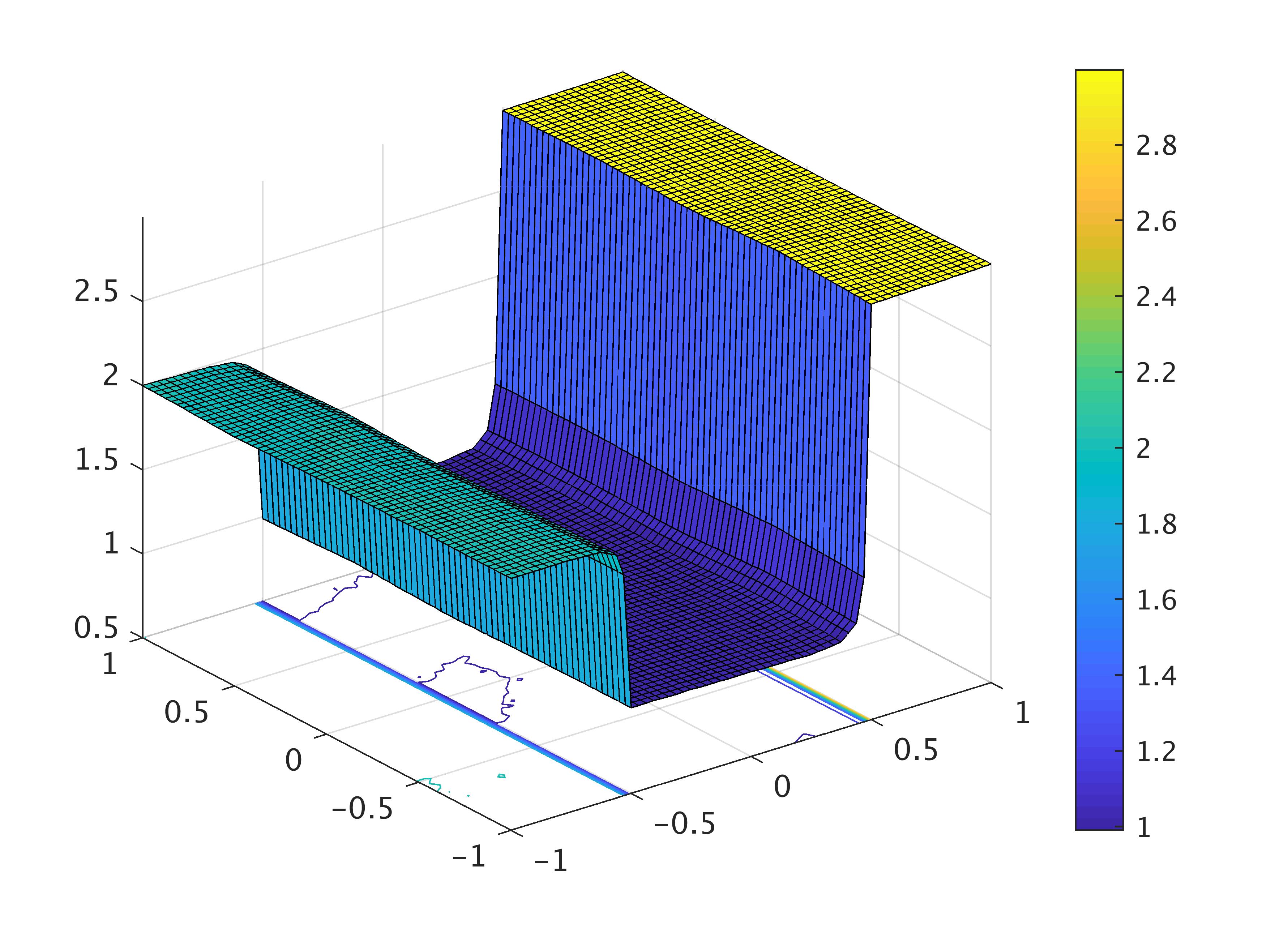
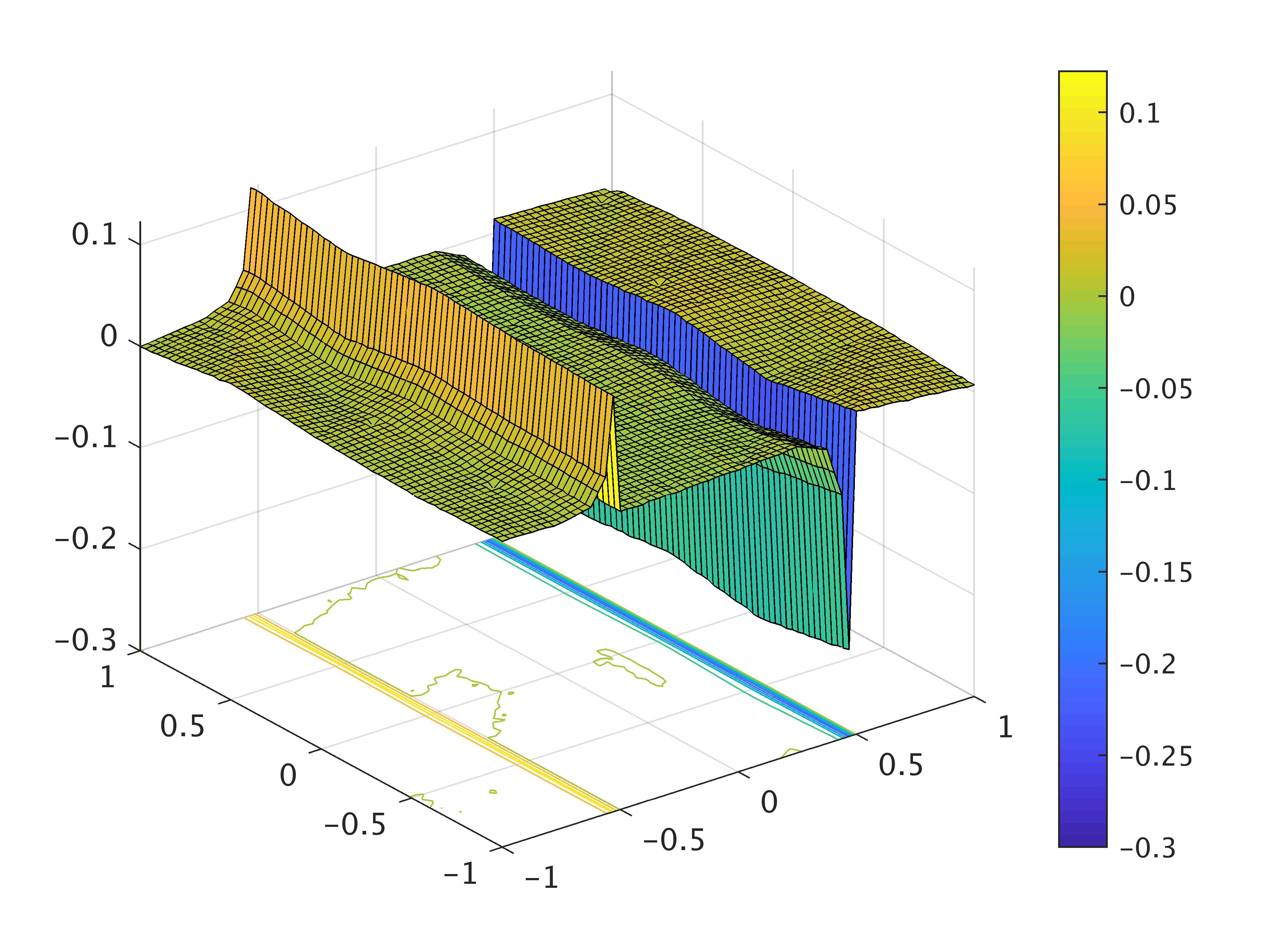
Figure 1: Computed diffusion $q_{\tau}$ (left) and the difference from the exact diffusion $q^{\dagger}-q_{\tau}$ (right).

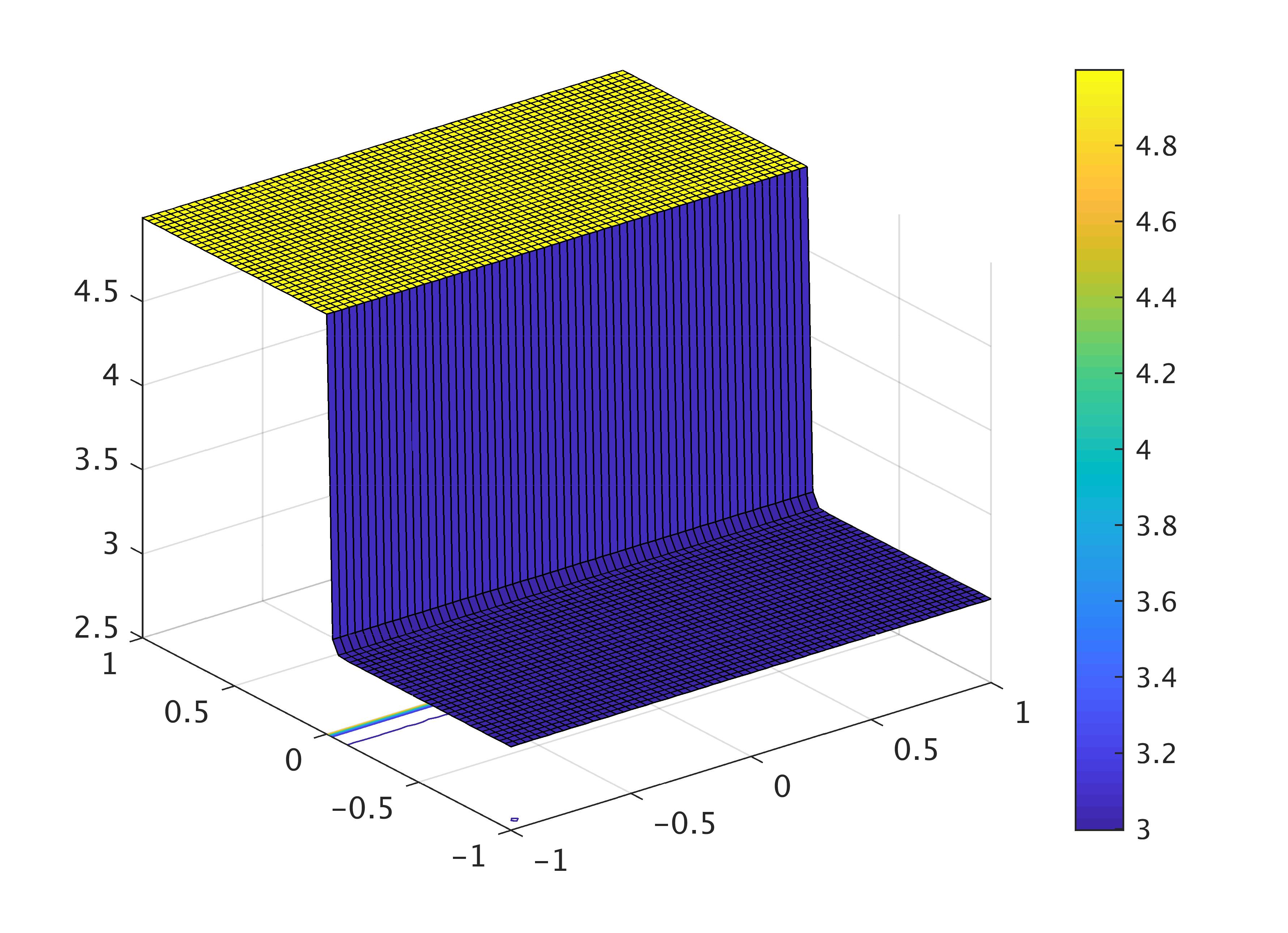
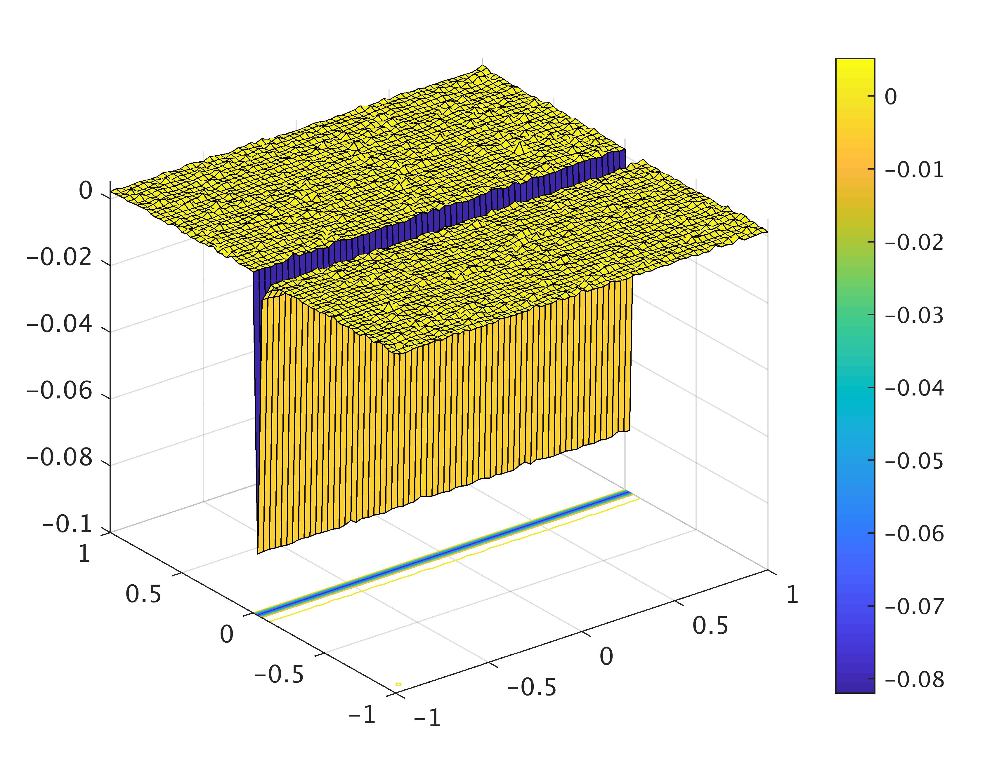
Figure 2: Computed reaction $a_{\tau}$ (left) and the difference from the exact reaction $a^{\dagger}-a_{\tau}$ (right).

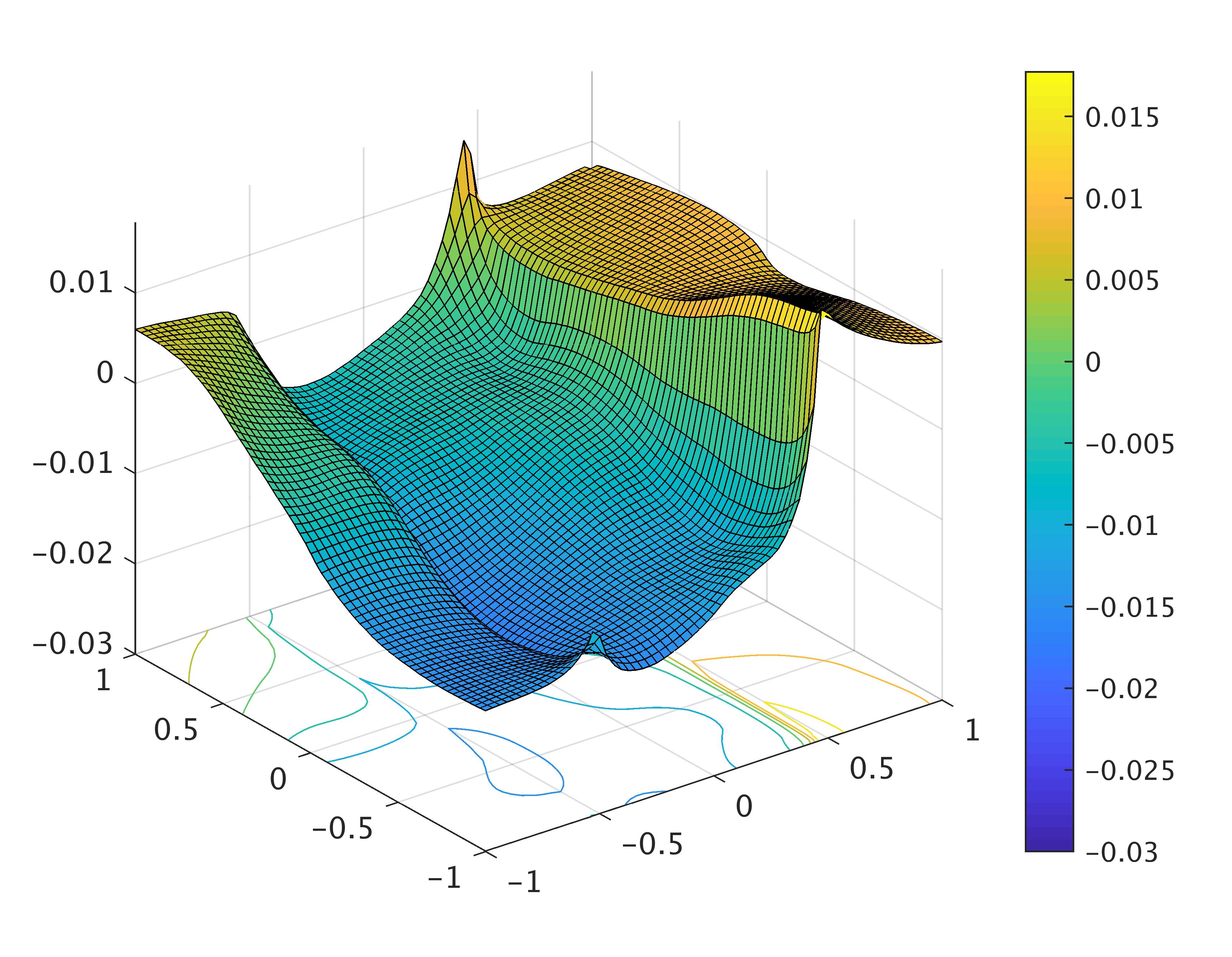
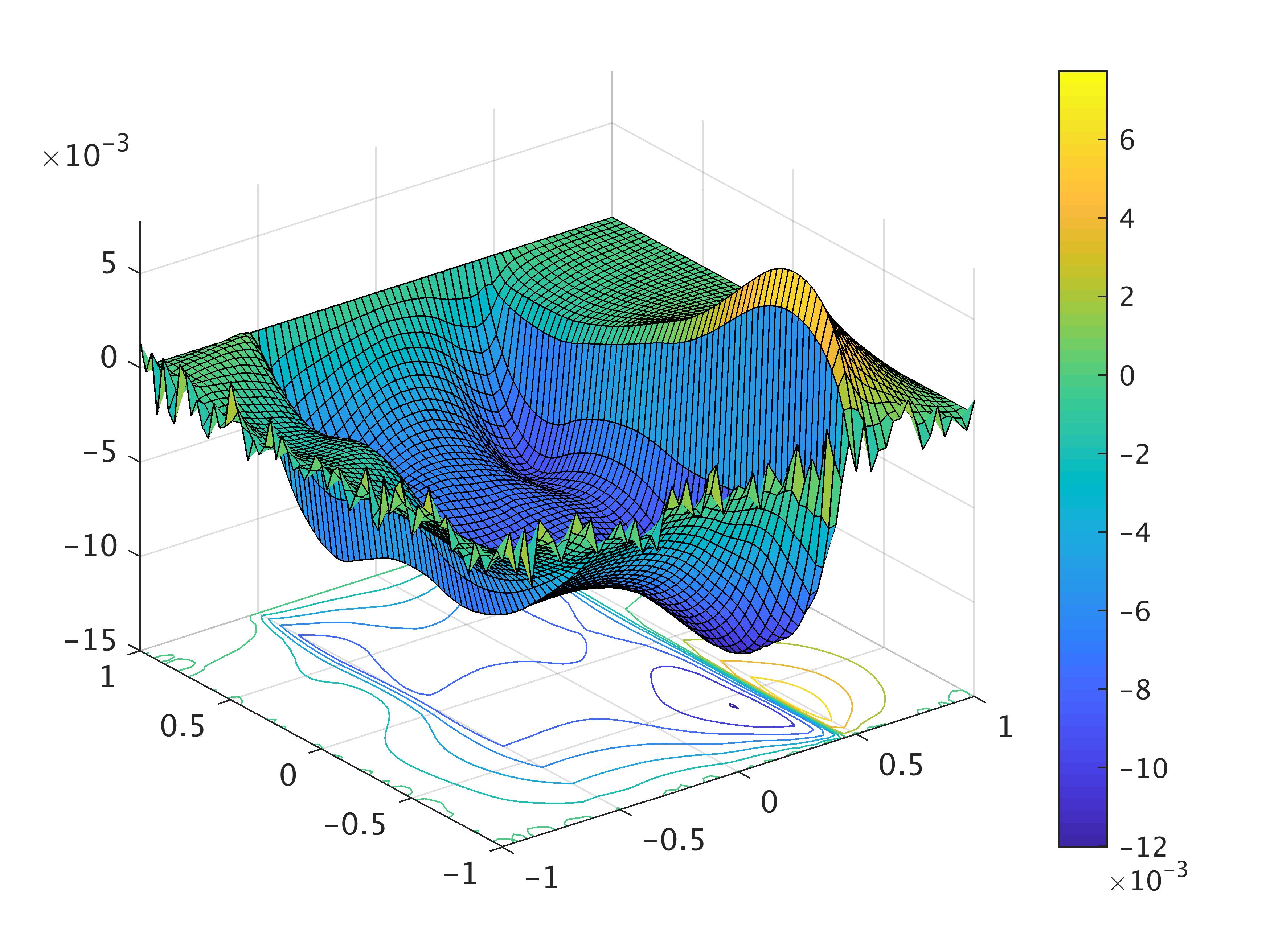
Figure 3: Differences $N^{h_{\tau}}_{j^{\dagger}}(q^{\dagger},a^{\dagger})-N^{h_{\tau}}_{j_{\delta}}(q_{\tau},a_{\tau})$ (left) and $D^{h_{\tau}}_{\widehat{g}^{\dagger}}(q^{\dagger},a^{\dagger})-D^{h_{\tau}}_{g^{\dagger}_{\delta}}(q_{\tau},a_{\tau})$ (right).

Example 6.2.

We here take $\theta$ in (6.7) to be independent of the refinement levels $\tau$ by

$$\theta=0.1,0.05,~{}\mbox{and}~{}0.01$$

and the noisy levels are then computed from the formula (6.8). In the Table 2 we present the computational results for the finest refinement $\tau=64$. As the previous implementation we observe a decrease of all errors as noisy levels get smaller.

Numerical result for different values of $\theta$ at $\tau=64$
$\theta$	$\delta$	$E_{q,a}$	$E_{N}$	$E_{M}$	$E_{D}$
0.01	3.0011e-2	9.4379e-2	3.0362e-2	2.3549e-2	1.2186e-2
0.05	0.1368	0.2115	7.1326e-2	5.0149e-2	2.6825e-2
0.1	0.2317	0.3921	0.1485	0.1121	5.2141e-2

Table 2: Numerical result for different values of $\theta$ independent of the refinement levels at the finest level $\tau=64$.

We in the top two figures of Figure 4 present the difference between the exact diffusion (respectively, reaction) and the computed diffusion (respectively, reaction) for $\theta=0.01$, while the similar illustrations for $\theta=0.05$ are performed in the bottom two figures.

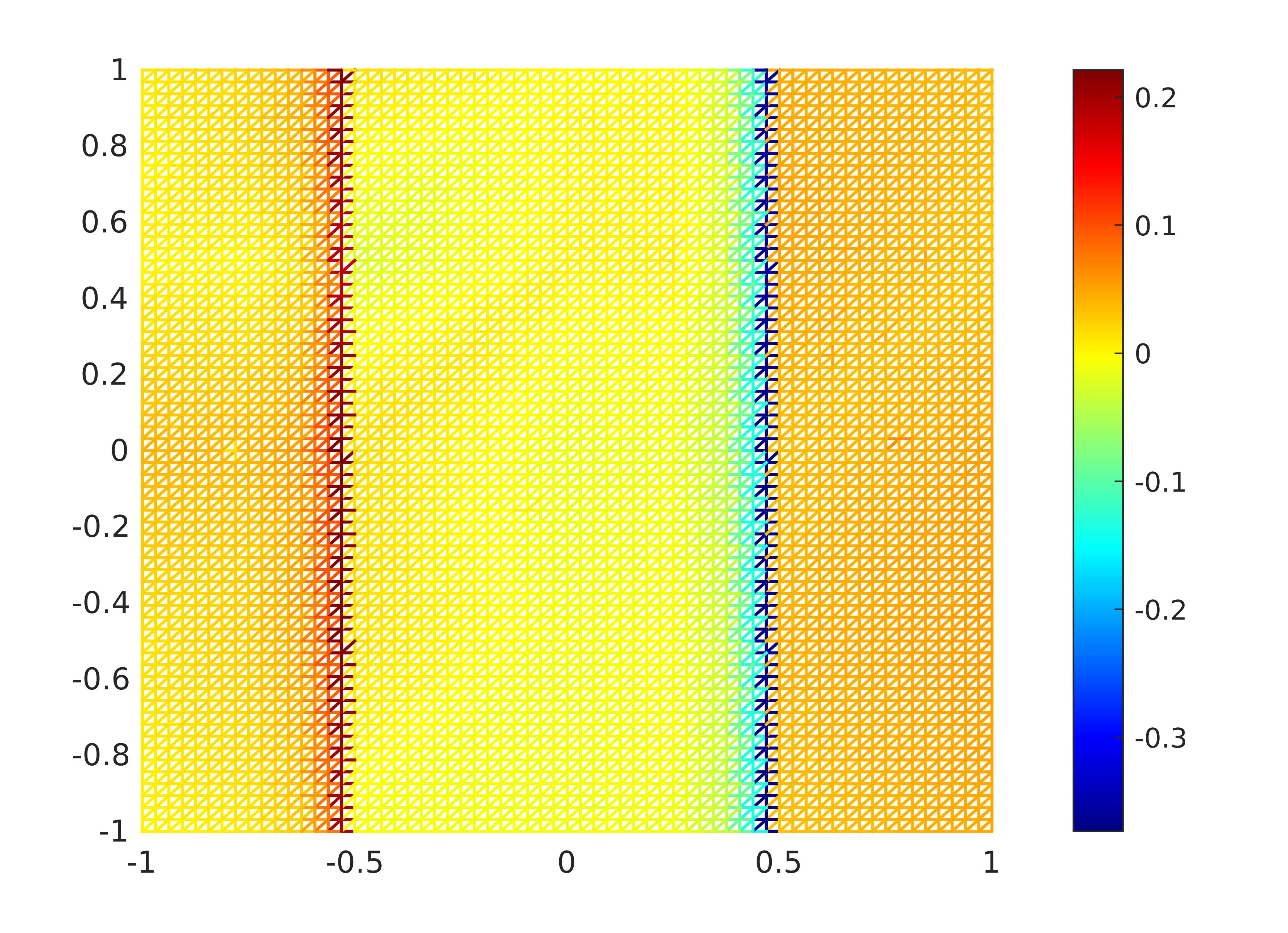
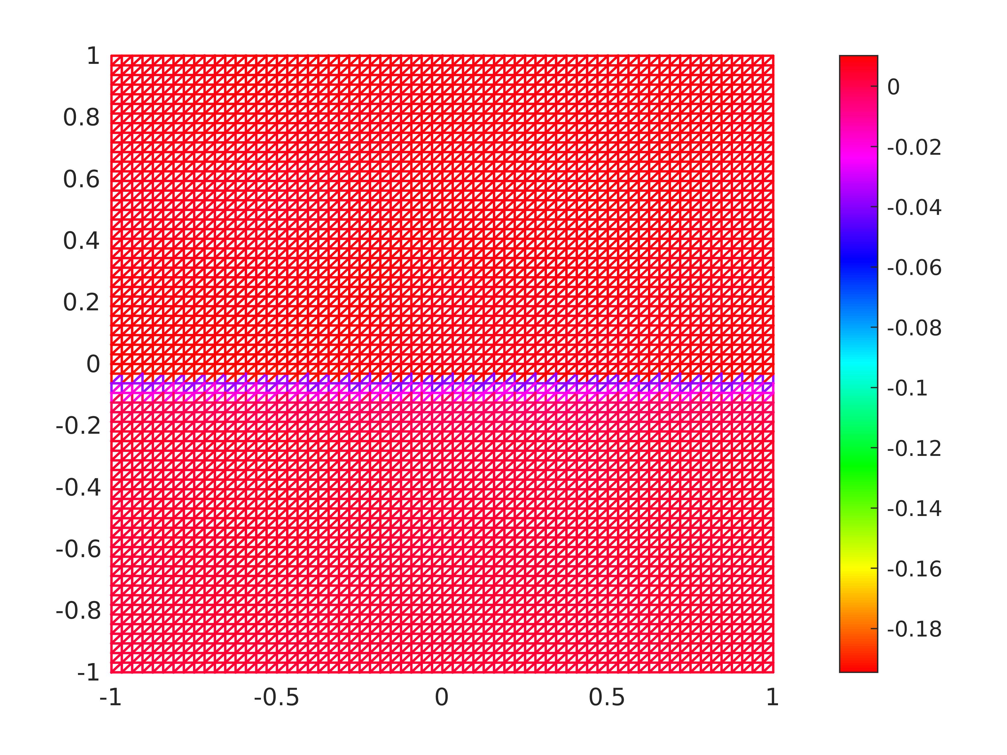
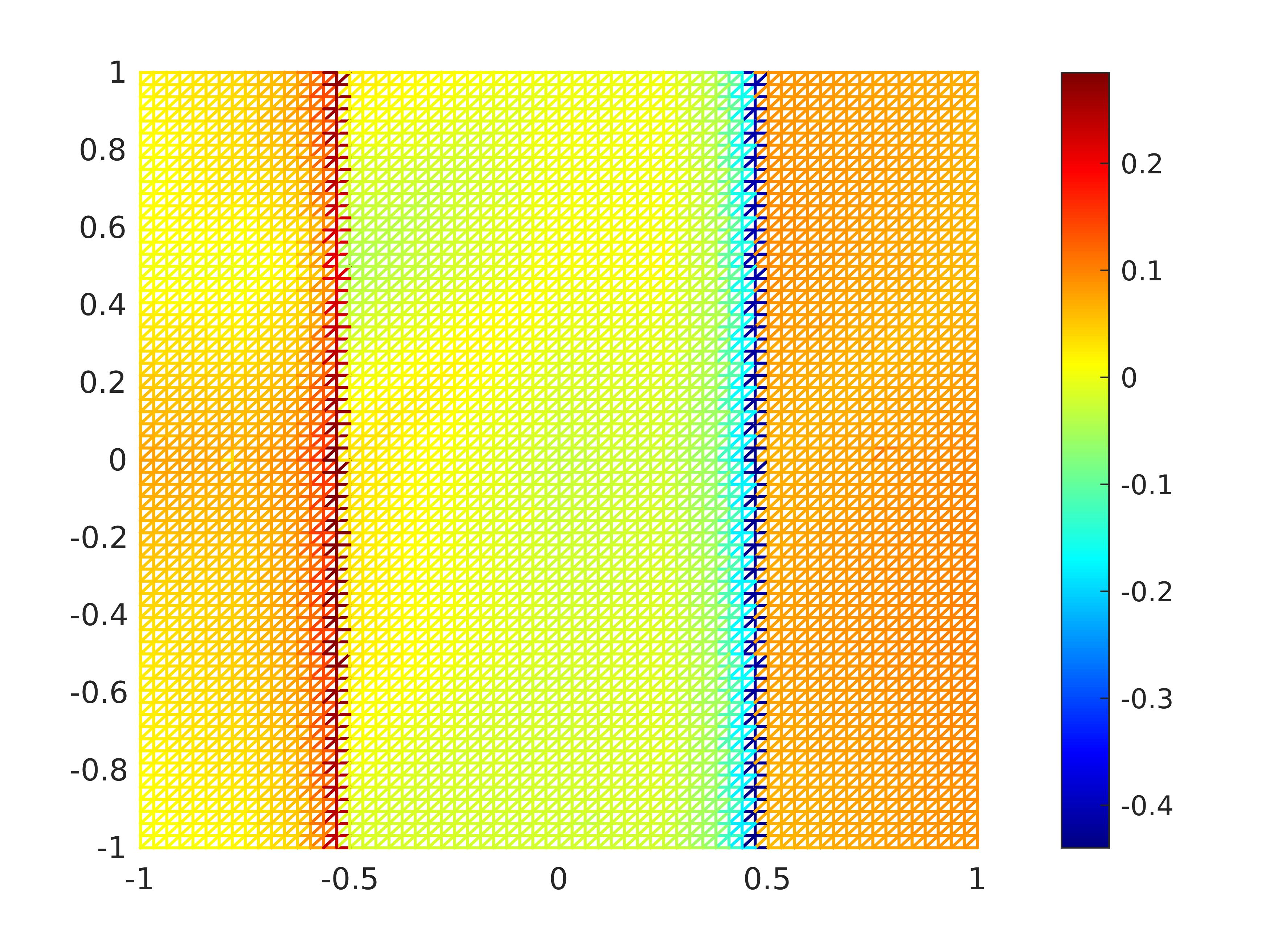
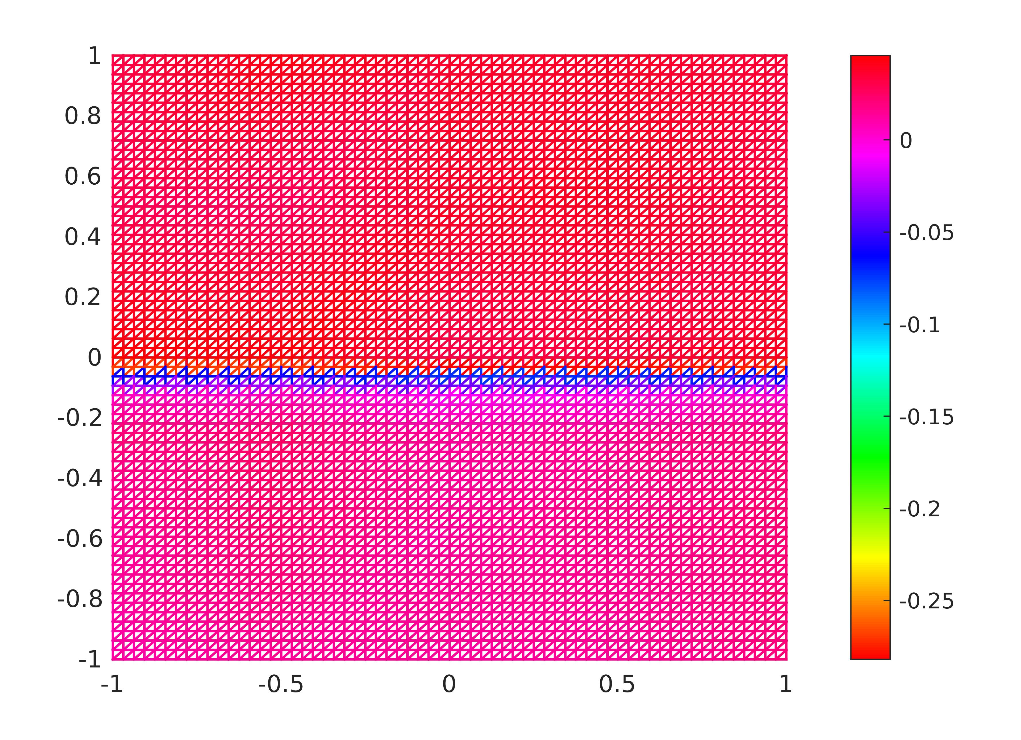
Figure 4: Differences between the exact diffusion (respectively, reaction) and the computed diffusion (respectively, reaction): $\theta=0.01$ (top two figures) and $\theta=0.05$ (bottom two figures).

Example 6.3.

Finally, we consider the case of multiple measurements. Assume that $I$ multiple measurements $\left(j_{\delta}^{i},g_{\delta}^{i}\right)_{i=1,\ldots,I}$ on $\Gamma$ are available. With these datum at hand, we examine the minimization problem

$$\min_{(q,a)\in Q^{h}_{ad}\times A^{h}_{ad}}\widehat{\Upsilon}^{h}_{\delta,\rho}(q,a),$$

where

$$\widehat{\Upsilon}^{h}_{\delta,\rho}(q,a) :=\widehat{J}^{h}_{\delta}(q,a)+\rho R(q,a)\quad\mbox{and}$$

$$\widehat{J}^{h}_{\delta}(q,a) :=\frac{1}{I}\sum_{i=1}^{I}\Bigg{(}\int_{\Omega}q\left|\nabla\big{(}N^{h}_{j^{i}_{\delta}}(q,a)-M^{h}_{g^{i}_{\delta}}(q,a)\big{)}\right|^{2}dx+\int_{\Omega}a\big{(}N^{h}_{j^{i}_{\delta}}(q,a)-M^{h}_{g^{i}_{\delta}}(q,a)\big{)}^{2}dx$$

$$~{}\quad+\int_{\partial\Omega}\sigma\big{(}N^{h}_{j^{i}_{\delta}}(q,a)-M^{h}_{g^{i}_{\delta}}(q,a)\big{)}^{2}ds\Bigg{)},$$

which admits a minimizer $\big{(}\widehat{q}^{h}_{\delta,\rho},\widehat{a}^{h}_{\delta,\rho}\big{)}$.

We now rewrite the exact boundary data $\left(j^{\dagger},g^{\dagger}\right)$ in (6.5) – (6.6) as

$$j^{\dagger}_{(A,B,C,D)}:=A\cdot\chi_{(0,1)\times\{-1\}}+B\cdot\chi_{[-1,0]\times\{-1\}}+C\cdot\chi_{\{-1\}\times(-1,0]}+D\cdot\chi_{\{-1\}\times(0,1)}$$

and $g^{\dagger}_{(A,B,C,D)}:=\gamma_{|\Gamma}N_{j^{\dagger}_{(A,B,C,D)}}(q^{\dagger},a^{\dagger})$, which depend on the constants $(A,B,C,D)$. As in (6.7), the noisy observations are assumed to be given by

$$\left(j^{(A,B,C,D)}_{\delta},g^{(A,B,C,D)}_{\delta}\right)=\left(j^{\dagger}_{(A,B,C,D)}+r\theta,g^{\dagger}_{(A,B,C,D)}+r\theta\right).$$ (6.9)

In the case $(A,B,C,D)=(-1,1,-2,3)$ we obtain a single noisy measurement, i.e. $I=1$. We now fix $D=3$, and let $(A,B,C)$ take all permutations $\mathcal{S}_{3}$ of the set $\{-1,1,-2\}$, the equation (6.9) then generates $I=6$ measurements. Likewise, if $(A,B,C,D)$ takes all permutations $\mathcal{S}_{4}$ of $\{-1,1,-2,3\}$ we have $I=16$ measurements.

The noisy level is given by

$$\delta=\begin{cases}\big{\|}j^{(-1,1,-2,3)}_{\delta}-j^{\dagger}_{(-1,1,-2,3)}\big{\|}_{L^{2}(\Gamma)}+\big{\|}g^{(-1,1,-2,3)}_{\delta}-g^{\dagger}_{(-1,1,-2,3)}\big{\|}_{L^{2}(\Gamma)}\mbox{~{}if~{}}(A,B,C,D)=(-1,1,-2,3),\\ \dfrac{1}{6}\sum_{(A,B,C)\in\mathcal{S}_{3}}\big{\|}j^{(A,B,C,3)}_{\delta}-j^{\dagger}_{(A,B,C,3)}\big{\|}_{L^{2}(\Gamma)}+\big{\|}g^{(A,B,C,3)}_{\delta}-g^{\dagger}_{(A,B,C,3)}\big{\|}_{L^{2}(\Gamma)}\mbox{~{}if~{}}D=3,\\ \dfrac{1}{16}\sum_{(A,B,C,D)\in\mathcal{S}_{4}}\big{\|}j^{(A,B,C,D)}_{\delta}-j^{\dagger}_{(A,B,C,D)}\big{\|}_{L^{2}(\Gamma)}+\big{\|}g^{(A,B,C,D)}_{\delta}-g^{\dagger}_{(A,B,C,D)}\big{\|}_{L^{2}(\Gamma)}.\end{cases}$$

A computation with $\theta=0.1$ and $\tau=64$ shows $\delta=0.2317$. The correspondingly numerical result for the multiple measurement case is presented in the Table 3, where its first line is copied from the last one of Table 2. We observe that the use of multiple measurements improves the obtaining numerical solutions in case of the large noise level, as can be seen all errors decrease oppositely with the increase of the number of measurements.

Errors for multiple measurements
Number of measurements $I$	$E_{q,a}$	$E_{N}$	$E_{M}$	$E_{D}$
1	0.3921	0.1485	0.1121	5.2141e-2
6	0.2849	8.4842e-2	6.0352e-2	3.8542e-2
16	0.1609	4.7708e-2	3.3418e-2	1.9260e-2

Table 3: Errors for multiple measurements $I=1,6,16$ with $\theta=0.1$ and $\tau=64$, i.e. $\delta=0.2317$.

Finally, in Figure 5 – Figure 7 we perform the graphs of the computation, which include the differences between the exact coefficient and the computational one, i.e. $q^{\dagger}-q_{\tau}$ (left) and $a^{\dagger}-a_{\tau}$ (right). We would like to note that the computational errors occur much more at areas where the identified coefficients are discontinuous than others.

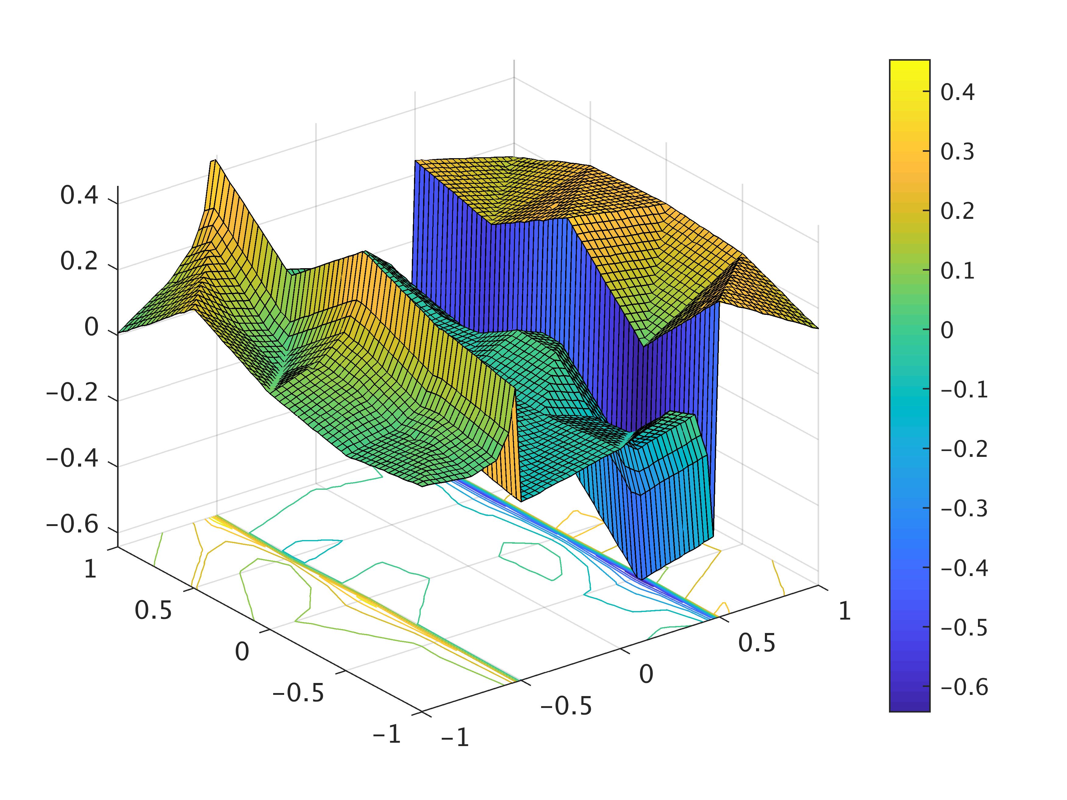
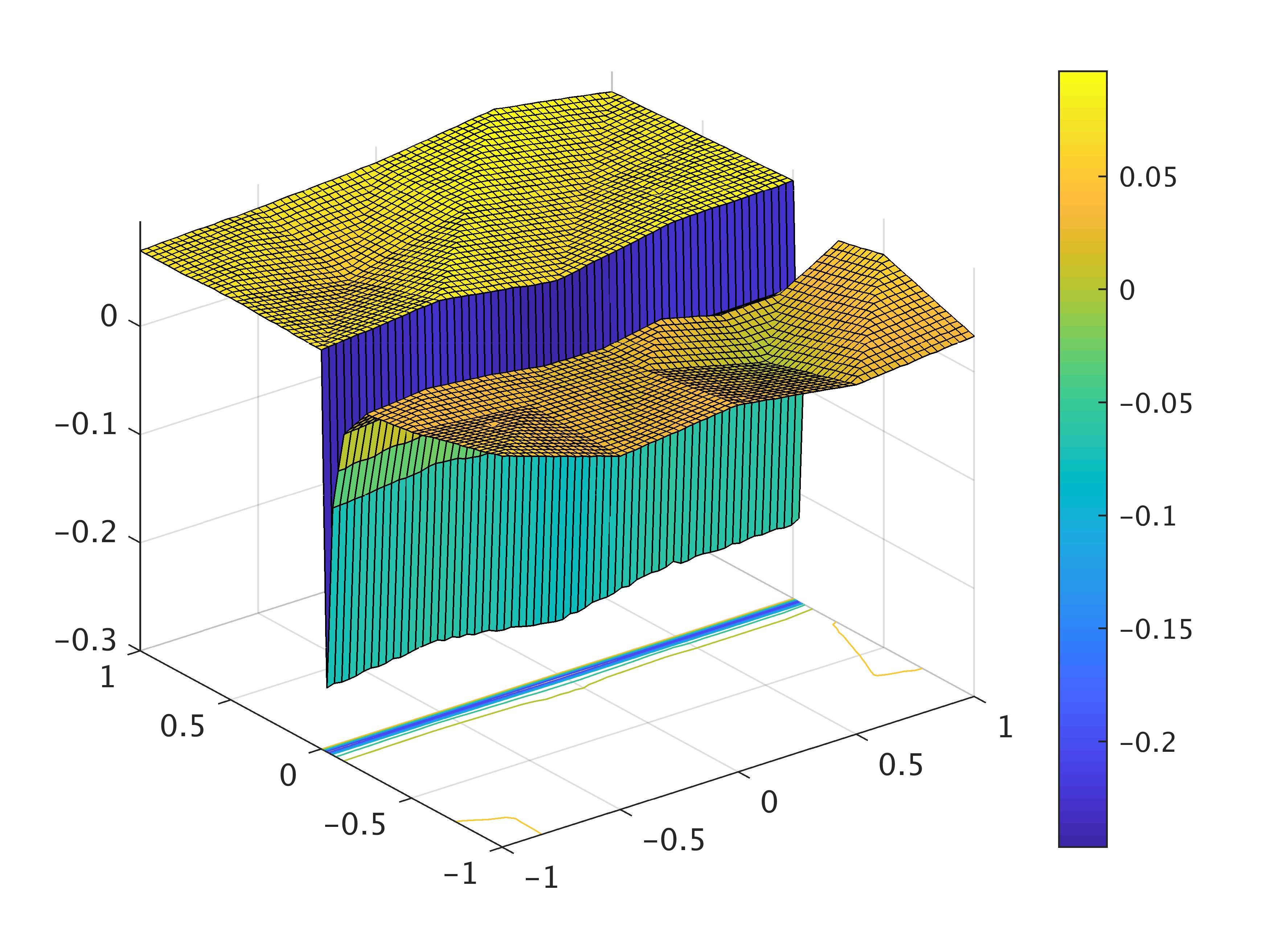
Figure 5: $I=1$: differences $q^{\dagger}-q_{\tau}$ (left) and $a^{\dagger}-a_{\tau}$ (right).

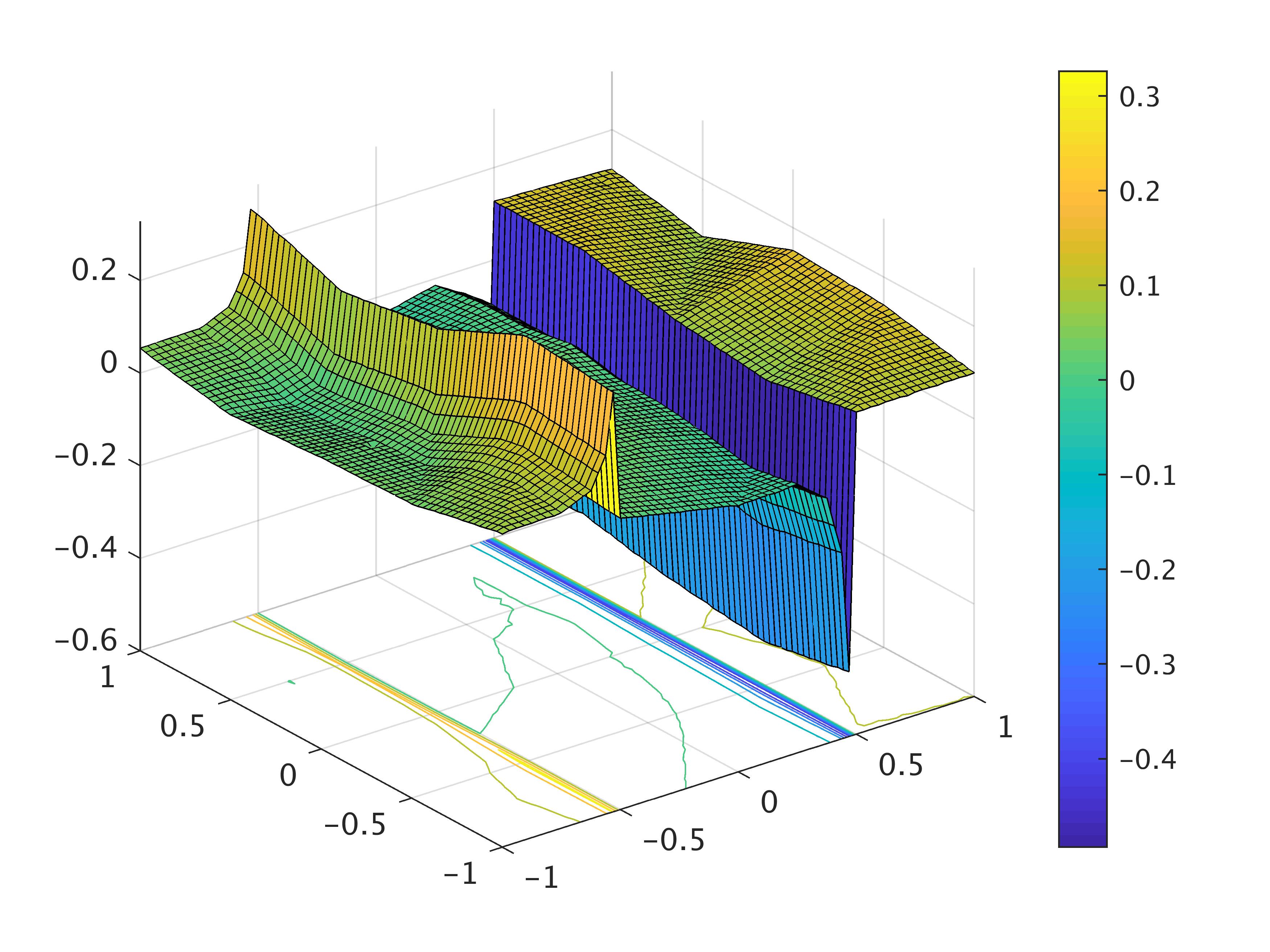
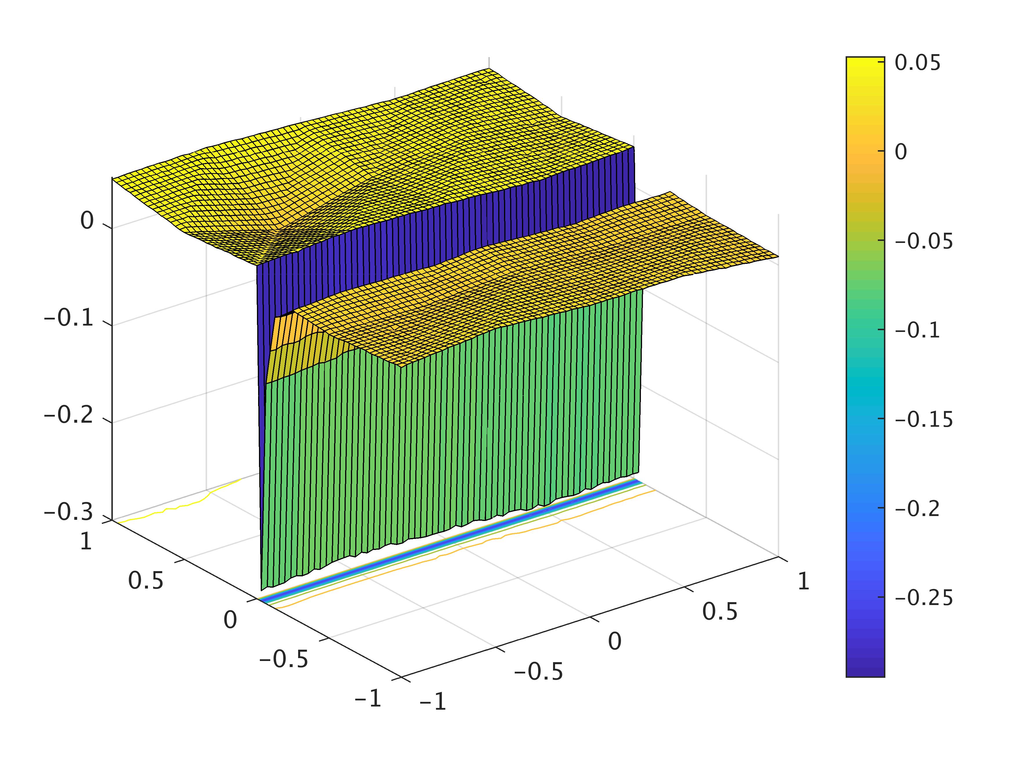
Figure 6: $I=6$: differences $q^{\dagger}-q_{\tau}$ (left) and $a^{\dagger}-a_{\tau}$ (right).

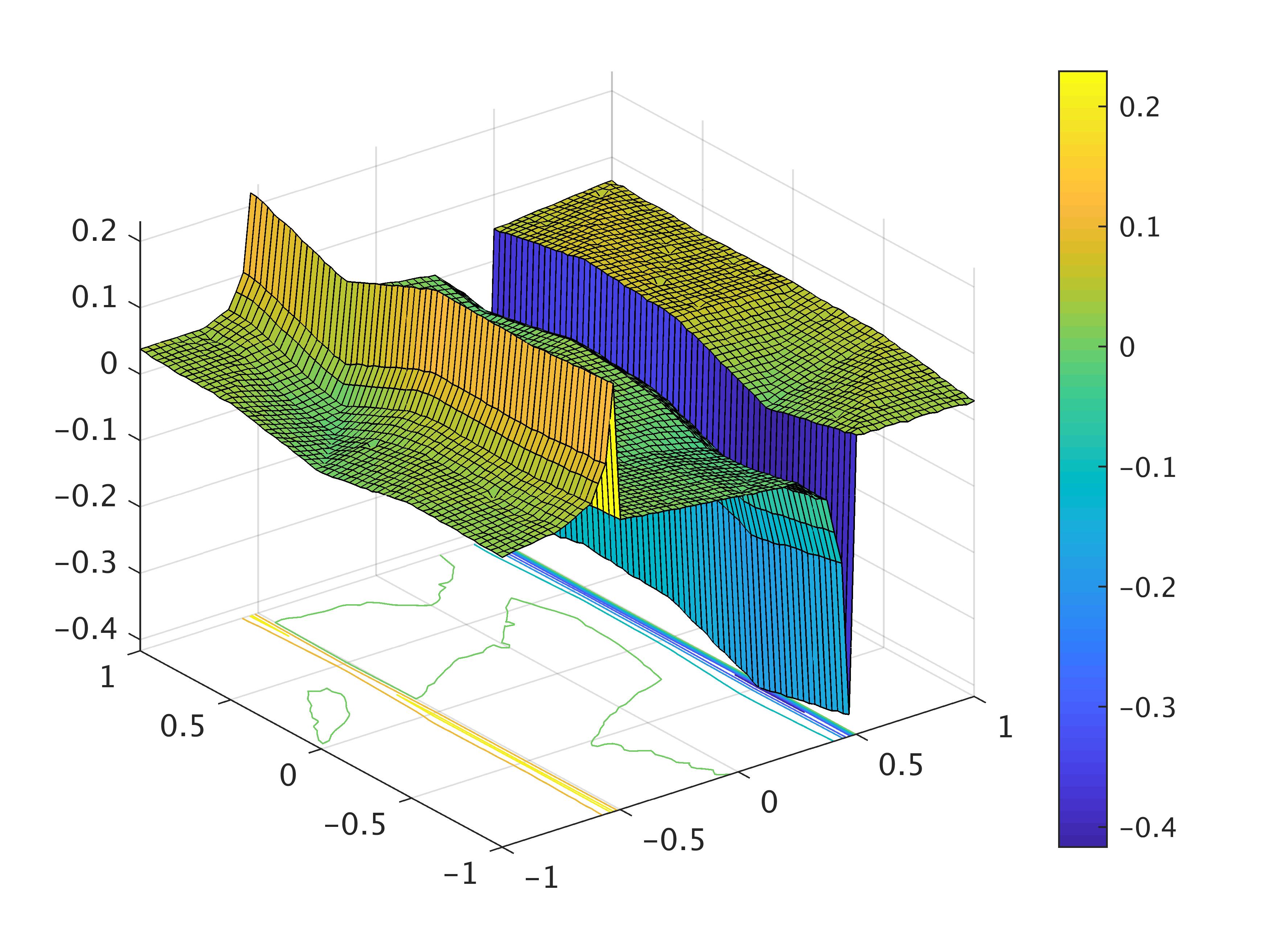
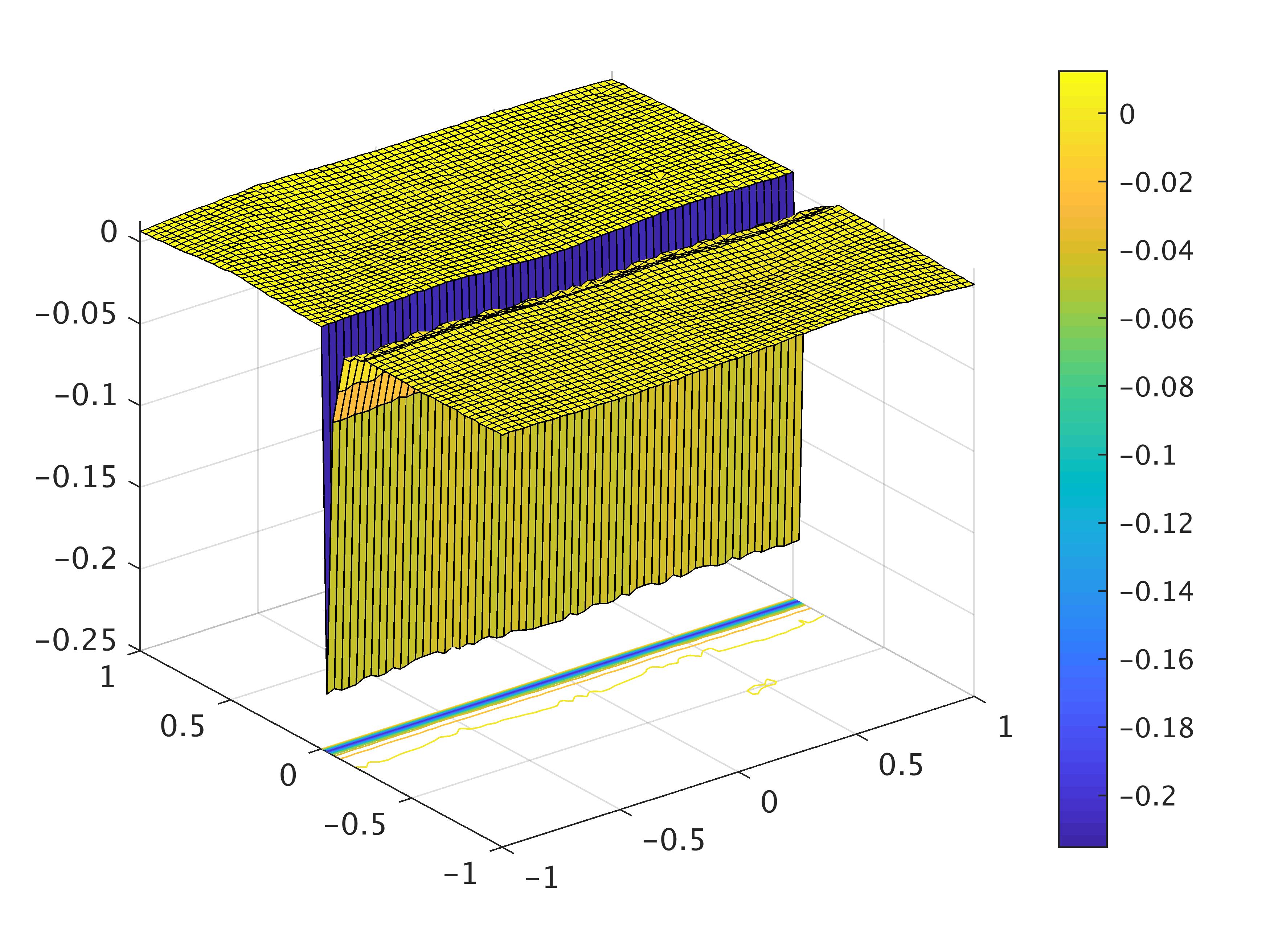
Figure 7: $I=16$: differences $q^{\dagger}-q_{\tau}$ (left) and $a^{\dagger}-a_{\tau}$ (right).

Acknowledgements: The author would like to thank the referees and the editor for their valuable comments and suggestions which helped to improve our paper.

References

- [1] R. Acar, Identification of the coefficient in elliptic equations, SIAM J. Control Optim. 31(1993), 1221– 1244.
- [2] G. Alessandrini, An identification problem for an elliptic equation in two variables. Ann. Mat. Pura Appl. 145(1986), 265–296.
- [3] S. R. Arridge, Optical tomography in medical imaging, Inverse Problems 15(1999), R41–R93.
- [4] S. R. Arridge and W. R. B. Lionheart, Nonuniqueness in diffusion-based optical tomography, Optics Letters 23(1998), pp. 882–884.
- [5] S. R. Arridge and J. C. Schotland, Optical tomography: forward and inverse problems, Inverse Problems 25(2009), 123010 (59pp).
- [6] K. Astala and L. Päivärinta, Calderón’s inverse conductivity problem in the plane, Ann. Math. 163(2006), pp. 265–299.
- [7] H. Attouch, G. Buttazzo and G. Michaille, Variational Analysis in Sobolev and BV Space, Philadelphia: SIAM, 2006.
- [8] J. Banasiak and G. F. Roach, On mixed boundary value problems of Dirichlet oblique-derivative type in plane domains with piecewise differentiable boundary, J. Math. Anal. Appl. 79(1989), 111–131.
- [9] S. Bartels, R. H. Nochetto and A. J. Salgado, Discrete TV flows without regularization, SIAM J. Numer. Anal. 52(2014), pp. 363–385.
- [10] J. Baumeister and K. Kunisch, Identifiability and stability of a two-parameter estimation problem. Appl. Anal. 40(1991), No. 4, 263–279.
- [11] L. Blank and C. Rupprecht, An extension of the projected gradient method to a Banach space setting with application in structural topology optimization, SIAM J. Control Optim. 55(2017), pp. 1481–1499.
- [12] D. A. Boas, A fundamental limitation of linearized algorithms for diffuse optical tomography, Optics Express 1(1997), 404–413.
- [13] L. Borcea, Electrical impedance tomography, Inverse Problems 18(2002), 99–136.
- [14] L. M. Bregman, The relaxation of finding the common points of convex sets and its application to the solution of problems in convex programming, USSR Comput. Math. Math. Phys. 7(1967), pp. 200–217.
- [15] S. Brenner and R. Scott, The Mathematical Theory of Finite Element Methods, New York: Springer, 1994.
- [16] B. H. Brown, Electrical impedance tomography (EIT): a review, Journal of Medical Engineering & Technology 27(2003), pp. 97–108.
- [17] R. M. Brown and R. H. Torres, Uniqueness in the inverse conductivity problem for conductivities with 3/2 derivatives in , , J. Fourier Anal. Appl. 9(2003), pp. 563–574.
- [18] R. M. Brown and G. A. Uhlmann, Uniqueness in the inverse conductivity problem for nonsmooth conductivities in two dimensions, Comm. Partial Differential Equations 22(1997), pp. 1009–1027.
- [19] M. Burger and S. Osher, Convergence rates of convex variational regularization, Inverse Problems 20(2004), 1411–1421.
- [20] M. Burger and S. Osher, A guide to the TV zoo, in: Level-Set and PDE-based Reconstruction Methods, M.Burger, S.Osher, eds.: Springer, 2013.
- [21] N. Cao, A. Nehorai, and M. Jacob, Image reconstruction for diffuse optical tomography using sparsity regularization and expectation-maximization algorithm, Optics Express 15(2007), 13695–13708.
- [22] T. F. Chan and X. C. Tai, Identification of discontinuous coefficients in elliptic problems using total variation regularization SIAM J. Sci. Comput. 25(2003), 881–904.
- [23] T. F. Chan and X. C. Tai, Level set and total variation regularization for elliptic inverse problems with discontinuous coefficients Joural of Computational Physics 193(2003), 40–66.
- [24] G. Chavent and K. Kunisch, Regularization of linear least squares problems by total bounded variation, ESIAM Contr. Optim. Calc. Var. 2(1997), pp. 359–376.
- [25] G. Chavent and K. Kunisch, The output least squares identifiability of the diffusion coefficient from an -observation in a 2-D elliptic equation ESAIM Control Optim. Calc. Var. 8(2002), 423–440.
- [26] Z. Chen and J. Zou, An augmented Lagrangian method for identifying discontinuous parameters in elliptic systems SIAM J. Control And Optim. 37(1999), no. 3, 892–910.
- [27] M. Cheney, D. Isaacson and J. C. Newell, Electrical impedance tomography, SIAM Rev. 41(1999), pp. 85–101.
- [28] E. Crossen, M. S. Gockenbach, B. Jadamba, A. A. Khan and B. Winkler, An equation error approach for the elasticity imaging inverse problem for predicting tumor location, Comput. Math. Appl. 2014(67), 122–135.
- [29] A. Dijkstra, B. Brown, N. Harris, D. Barber, and D. Endbrooke, Review: Clinical applications of electrical impedance tomography, J. Med. Eng. Technol. 17(1993), 89–98.
- [30] D. C. Dobson, Recovery of blocky images in electrical impedance tomography, in Inverse Problems in Medical Imaging and Nondestructive Testing, H. W. Engl, A. K. Louis, and W. Rundell, eds.: Springer, 1997, pp. 43–64.
- [31] T. Durduran, R. Choe, W. B. Baker and A. G. Yodh, Diffuse optics for tissue monitoring and tomography, Rep. Prog. Phys. 73(2010), 076701 (43pp).
- [32] I. Ekeland and R. Temam, Convex Analysis and Variational Problems, New York: American Elsevier Publishing Company Inc., 1976.
- [33] L. C. Evans and R. F. Gariepy, Measure Theory and Fine Properties of Functions. CRC Press, 1992.
- [34] R. Falk, Error estimates for the numerical identification of a variable coefficient Math. Comput. 40(1983), 537–546.
- [35] A. P. Gibson, J. C. Hebden and S. R. Arridge, Recent advances in diffuse optical imaging, Phys. Med. Biol. 50(2005), R1–R43.
- [36] E. Giusti, Minimal Surfaces and Functions of Bounded Variation, Boston: Birkhäuser, 1984.
- [37] P. Grisvard, Elliptic Problems in Nonsmooth Domains, Boston: Pitman, 1985.
- [38] D. N. Hào and T. N. T. Quyen, Convergence rates for Tikhonov regularization of coefficient identification problems in Laplace-type equations, Inverse Problems 26(2010), 125014 (23pp).
- [39] D. N. Hào and T. N. T. Quyen, Convergence rates for total variation regularization of coefficient identification problems in elliptic equations I, Inverse Problems 27(2011), 075008 (28pp).
- [40] D. N. Hào and T. N. T. Quyen, Convergence rates for total variation regularization of coefficient identification problems in elliptic equations II, J. Math. Anal. Appl. 388(2012), 593–616.
- [41] D. N. Hào and T. N. T. Quyen, Convergence rates for Tikhonov regularization of a two-coefficient identification problem in an elliptic boundary value problem, Numer. Math. 120(2012), 45–77.
- [42] B. Harrach, On uniqueness in diffuse optical tomography, Inverse Problems 25 (2009), 055010 pp. 14.
- [43] B. Harrach, Simultaneous determination of the diffusion and absorption coefficient from boundary data, Inverse Problems Imaging 6(2012), 663–679.
- [44] J. C. Hebden, S. R. Arridge and D. T. Delpy, Optical imaging in medicine: II. Modelling and reconstruction, Phys. Med. Biol. 42(1997), 841–853.
- [45] T. Hein and M. Meyer, Simultaneous identification of independent parameters in elliptic equations–numerical studies. J. Inv. Ill-Posed Problems 16(2008), 417–433.
- [46] J. Heino and E. Somersalo, Estimation of optical absorption in anisotropic background, Inverse Problems 18(2002), 559–573.
- [47] M. Hinze, B. Kaltenbacher and T. N. T. Quyen, Identifying conductivity in electrical impedance tomography with total variation regularization, Numerische Mathematik 138(2018), pp. 723–765.
- [48] M. Hinze, R. Pinnau, M. Ulbrich, S. Ulbrich, Optimization with PDE Constraints, Series Mathematical Modelling: Theory and Applications, Vol. 23: Springer, 2009.
- [49] Y. Hoshi and Y. Yamada, Overview of diffuse optical tomography and its clinical applications, J. Biomedical Optics 21(9), 091312.
- [50] K. Ito and K. Kunisch, Lagrange Multiplier Approach to Variational Problems and Applications. Advances in Design and Control, 15. Society for Industrial and Applied Mathematics (SIAM), Philadelphia, PA, 2008.
- [51] M. F. Al-Jamal and M. S. Gockenbach, Stability and error estimates for an equation error method for elliptic equations, Inverse Problems 28(2012), 095006 (15pp).
- [52] Y. L. Keung and J. Zou, An efficient linear solver for nonlinear parameter identification problems, SIAM J. Sci. Comput 22(2000), 1511–1526.
- [53] A. Kienle, L. Lilge, M. S. Patterson, R. Hibst, R. Steiner and B. C. Wilson, Spatially resolved absolute diffuse reflectance measurements for noninvasive determination of the optical scattering and absorption coefficients of biological tissue, Applied Optics 35(1996), 2304–2314.
- [54] K. C. Kiwiel, Proximal minimization methods with generalized Bregman functions, SIAM J. Control Optim. 35(1997), 1142–1168.
- [55] I. Knowles, A variational algorithm for electrical impedance tomography, Inverse Problems 14(1998), 1513–1525.
- [56] R. V. Kohn and A. McKenney, Numerical implementation of a variational method for electrical impedance tomography, Inverse Problems 6(1990) 389–414.
- [57] R. V. Kohn and B. D. Lowe, A variational method for parameter identification, RAIRO Modél. Math. Anal. Numér 22(1988), 119–158.
- [58] R. V. Kohn and M. Vogelius, Determining Conductivity by Boundary Measurements, Comm. Pure Appl. Math. 37(1984), 289–298.
- [59] R. V. Kohn and M. Vogelius, Determining conductivity by boundary measurements. II. Interior results, Comm. Pure Appl. Math. 38(1985), 643–667.
- [60] R. V. Kohn and M. Vogelius, Relaxation of a variational method for impedance computed tomography, Comm. Pure Appl. Math. 40(1987), 745–777.
- [61] A. Lechleiter and A. Rieder, Newton regularizations for impedance tomography: convergence by local injectivity, Inverse Problems 24(2008), 065009 (18pp).
- [62] O. Lee and J. C. Ye, Joint sparsity-driven non-iterative simultaneous reconstruction of absorption and scattering in diffuse optical tomography, Optics Express 21(2013), 26589–26604.
- [63] J. L. Mueller and S. Siltanen, Linear and Nonlinear Inverse Problems with Practical Applications, Philadelphia: SIAM, 2012.
- [64] A. Nachman, Global uniqueness for a two-dimensional inverse boundary value problem, Ann. Math. 143(1996), pp. 71–96.
- [65] L. Päivärinta, A. Panchenko, and G. Uhlmann, Complex geometric optics solutions for Lipschitz conductivities, Rev. Mat. Iberoamericana 19(2003), pp. 57–72.
- [66] C. Pechstein, Finite and Boundary Element Tearing and Interconnecting Solvers for Multiscale Problems, Heidelberg New York Dordrecht London: Springer, 2010.
- [67] B. W. Pogue, M. S. Patterson, H. Jiang and K. D. Paulsen, Initial assessment of s simple system for frequency domain diffuse optical tomography, Phys. Med. Biol. 40(1995), 1709–1729.
- [68] T. N. T. Quyen, Finite element analysis for identifying the reaction coefficient in PDE from boundary observations, Appl. Numer. Math. 145(2019), pp. 297–314.
- [69] K. Ren, G. Bal and A. H. Hielscher, Transport- and diffusion-based optical tomography insmall domains: a comparative study, Applied Optics 46(2007), 6669–6679.
- [70] E. Resmerita and O. Scherzer, Error estimates for non-quadratic regularization and the relation to enhancement, Inverse Problems 22(2006), 801–814.
- [71] G. R. Richter, An inverse problem for the steady state diffusion equation. SIAM J. Appl. Math. 41(1981), 210–221.
- [72] L. I. Rudin, S. J. Osher and E. Fatemi, Nonlinear total variation based noise removal algorithms, Physica D 60(1992), pp. 259–268.
- [73] S. Sauter and C. Schwab, Boundary Element Methods (volume 39 of Springer series in Compuational Mathematics), Berlin: Springer, 2011.
- [74] J. Sylvester and G. Uhlmann, A global uniqueness theorem for an inverse boundary value problem, Ann. Math. 125(1987), pp. 153–169.
- [75] G. M. Troianiello, Elliptic differential equations and obstacle problems, New York: Plenum, 1987.
- [76] G. Uhlmann, Electrical impedance tomography and Calderón’s problem, Inverse Problems 25(2009), 123011 (39pp).
- [77] G. Vainikko and K. Kunisch, Identifiabilty of the transmissivity coefficient in an elliptic boundary value problem. Zeischrift für Analysis und ihre Anwendungen 12(1993), 327–341.
- [78] J. Zou, Numerical methods for elliptic inverse problems. Inter. J. Computer Math. 70(1998), 211-232.