Variations of the Godbillon–Vey invariant
of transversely parallelizable foliations

Abstract

We consider a $(2q+1)$-dimensional smooth manifold $M$ equipped with a $(q+1)$-dimensional, a priori non-integrable, distribution ${\cal D}$ and a $q$-vector field ${\bf T}=T_{1}\wedge\ldots\wedge T_{q}$, where $\{T_{i}\}$ are linearly independent vector fields transverse to ${\cal D}$. Using a $q$-form $\omega$ such that ${\cal D}=\ker\,\omega$ and $\omega({\bf T})=1$, we construct a $(2q+1)$-form analogous to that defining the Godbillon–Vey class of a $(q+1)$-dimensional foliation, and show how does this form depend on $\omega$ and ${\bf T}$. For a compatible Riemannian metric $g$ on $M$, we express this $(2q+1)$-form in terms of ${\bf T}$ and extrinsic geometry of ${\cal D}$ and normal distribution ${\cal D}^{\bot}$. We find Euler-Lagrange equations of associated functionals: for variable $(\omega,{\bf T})$ on $(M,g)$, and for variable metric on $(M,{\cal D})$, when distributions/foliations and forms are defined outside a “singularity set” under additional assumption of convergence of certain integrals. We show that for a harmonic distribution ${\cal D}^{\bot}$ such $(\omega,{\bf T})$ is critical, characterize critical pairs when ${\cal D}$ is integrable and find sufficient conditions for critical pairs when variations are among foliations, calculate the index form and consider examples of critical foliations among twisted products, Reeb foliations and transversely holomorphic flows.

Keywords: foliation, Godbillon–Vey invariant, variation, singularity, mean curvature, transversely holomorphic flow, twisted product

Mathematics Subject Classifications (2010) Primary 53C12; Secondary 53C21

Introduction

The Godbillon–Vey cohomology class $\mathrm{gv}({\cal F})$, which occurs in algebraic topology, differential geometry and their applications [24], was defined first for codimension-one foliations as a 3-cohomology class. It proved to be one of the most interesting characteristic classes associated to a foliated manifold. Its non-vanishing tells a lot about the dynamics of the foliation, e.g., implies the existence of resilient leaves. The Godbillon–Vey class has been the subject of numerous publications by most prominent topologists interested in the foliation theory. It is known that the Godbillon-Vey invariant is non-rigid, and in [18] we studied the Godbillon-Vey invariant from the point of view of the variational calculus. Then $\mathrm{gv}({\cal F})$ was extended for foliations of codimension $q>1$, [5, 13], and the paper generalizes the variational approach for such foliations.

If a codimension $q>1$ transversely oriented foliation ${\cal F}$ of a closed manifold $M$ is defined by the equation $\omega=0$ for some nowhere zero $q$-form $\omega$, then $\mathrm{gv}({\cal F})$ is the de Rham cohomology class of the closed $(2q+1)$-form $\eta\wedge(d\eta)^{q}$, where $\eta$ is a one-form obeying $d\omega=\omega\wedge\eta$. The integrability condition for the tangent distribution $T{\cal F}=\ker\omega:=\{X\in TM:\,\omega(X,\,\ldots)=0\}$, implies the existence of such $\eta$, while $\mathrm{gv}({\cal F})$ does not depend on the choice of $\omega$ and $\eta$. The Godbillon–Vey class measures some sort of “twisting” of the leaves, and it plays a crucial role in topology and dynamics of foliations, see e.g. [5, 11, 14, 20] and [15, Problem 10]. The complex Godbillon–Vey class, defined for transversely holomorphic foliations of real codimension $2q$, is often referred as the Bott class. If a smooth map $f:\bar{M}\to M$ is transverse to ${\cal F}$ on $M$ then $\mathrm{gv}(f^{*}{\cal F})=f^{*}\mathrm{gv}({\cal F})$, thus concordant foliations have the same Godbillon–Vey classes. When $\dim M=2q+1$ we get a Godbillon–Vey number:

$$\mathrm{gv}({\cal F})=\int_{M}\eta\wedge(d\eta)^{q}.$$ (1)

There exists one parameter family of foliations on $S^{3}$ with the Godbillon–Vey number taking all values in an interval (for the particular Reeb foliation this number is zero), hence $\mathrm{gv}({\cal F})$ is not a homotopy invariant. As in the codimension one case, the Godbillon–Vey number (1) is nonzero for various examples, and can even take on a continuum of values. Variations of (1) under deformations of ${\cal F}$ have been studied in [1]. Our variational approach differs from one mentioned above. In our earlier work [18] we defined a Godbillon–Vey type invariant for a pair consisting of an arbitrary, a priori non-integrable, plane field $\cal D$ and a transverse to it vector field $T$ on a Riemannian manifold $(M^{3},g)$, studied its dependence on $\cal D$, $T$ and $g$, found derivatives of the functional, characterized critical 2-dimensional foliations for different types of variations, proved sufficient conditions for critical pairs when ${\cal D}$ varies over integrable plane fields (foliations), found the index form of our variation problem, provided examples with Roussarie and Reeb foliations and twisted products.

Non-integrable distributions (subbundles of the tangent bundle $TM$) appear in many situations, e.g. on contact manifolds and in sub-Riemannian geometry. A codimension $q$ distribution ${\cal D}$ can be defined by a locally decomposable $q$-form $\omega$, that is $\omega=\omega_{1}\wedge\ldots\wedge\omega_{q}$ for some one-forms $\omega_{i}$ given in a neighborhood of a point $x\in M$. Indeed, let $g$ be any Riemannian metric on $M$ and $T_{i}\ (1\leq i\leq q)$ a local basis of the distribution ${\cal D}^{\bot}$ normal to ${\cal D}$. Then locally ${\cal D}=\ker\omega$, where $\omega=T_{1}^{\flat}\wedge\ldots\wedge T_{q}^{\flat}$. The “musical” isomorphisms $\sharp$ and $\flat$ “lower” and “raise” indices of rank one tensors on $(M,g)$.

A distribution is framed if its “normal bundle” $TM/{\cal D}$ is endowed with a trivialization. In this paper, we consider a manifold $M^{2q+1}$ equipped with a $(q+1)$-dimensional distribution ${\cal D}$ and linearly independent vector fields $T_{i}\ (i\leq q)$ transverse to ${\cal D}$. Hence, ${\cal D}^{\pitchfork}={\rm span}(T_{1},\ldots,T_{q})$ is a smooth distribution isomorphic to $TM/{\cal D}$. Our framed distribution ${\cal D}$ can be represented by a decomposable $q$-form $\omega=\omega_{1}\wedge\ldots\wedge\omega_{q}$, where $\omega_{i}$ are (not uniquely defined) one-forms. Indeed, there exists a compatible Riemannian metric $g=\langle\,\cdot\,,\cdot\,\rangle$ on $M$, i.e., the above vector fields $T_{i}\ (i\leq q)$ are orthonormal and all are orthogonal to ${\cal D}$. Denote by ${\rm Riem}(M,{\cal D},{\bf T})$ the space of all such metrics. Given compatible metric $g$, set $\omega_{i}=T_{i}^{\flat}$. Denote by ${\bf T}=T_{1}\wedge\ldots\wedge T_{q}$ a multivector on $M$.

Operation $\iota_{\,\bf T}$ is defined on a differential $r$-form $\alpha$ with $r\geq q$ by

$$\iota_{\,\bf T}\,\alpha:=\iota_{\,T_{q}}\ldots\iota_{\,T_{1}}\,\alpha=\alpha(T_{1},\ldots,T_{q},\cdot\,,\ldots\cdot).$$

For a decomposable $q$-form $\omega$ representing ${\cal D}$, one may assume the following normalization:

$$\iota_{\,\bf T}\,\omega=1.$$ (2)

In fact, a pair $(\omega,{\bf T})$ or $({\cal D},{\bf T})$, where ${\cal D}$ is represented by a decomposable $q$-form $\omega$ satisfying (2), is the main geometric structure considered here. We build a $1$-form $\eta$ depending on $(\omega,{\bf T})$,

$$\eta=\iota_{\,\bf T}\,d\omega,$$ (3)

which is analogous to that defined in [18] for $q=1$, and study the functional

$$\mathrm{gv}:(\omega,{\bf T})\mapsto\int_{M}\eta\wedge(d\eta)^{q}.$$ (4)

In a sense, our one-form $\eta$ arises from the best approximation of $(q+1)$-form $d\omega$ by the wedge-product of $\omega$ by a one-form, see Section 1. We provide variational formulas related to our construction and deduce Euler-Lagrange equations of (4) for variable pair $(\omega,{\bf T})$.

If $M$ is open, one may integrate over a relatively compact domain $G$ of $M$, containing supports of variations of $(\omega,\,{\bf T})$ or a Riemannian metric. Following ideas of [4, 23], we consider singular foliations, distributions and forms, that is those defined outside a “singularity set” $\Sigma$,

$$\Sigma=\{\mbox{a~{}finite union of pairwise disjoint closed submanifolds of codim. $\geq k$}\}$$

under an assumption of convergence of improper integrals $\int_{M}\|\beta\|^{p}\,{\rm d}V_{g}$ for suitable $(\dim M-1)$-forms $\beta$ defined on $M\smallsetminus\Sigma$ and some $p$ satisfying $(k-1)(p-1)\geq 1$.

The fundamental question is: What are the best almost product structures on a manifold? Such pairs $(\omega,{\bf T})$ (of the above question) are proposed to be among critical points of (4). We show that $(\omega,{\bf T})$ is critical when the distribution ${\cal D}^{\bot}$ is harmonic (with respect to compatible metric), characterize critical pairs when ${\cal D}$ is integrable and find sufficient conditions for critical pairs when variations are among foliations, calculate the index form and consider examples of critical foliations among twisted products, Reeb foliations and transversely holomorphic flows. We hope that the theory presented here can be used to deepen our knowledge of foliations as well as of topology of manifolds.

1 Construction

The Lie derivative of differential forms along vector fields can be generalized to a Lie derivative of differential forms along multivector fields, defined as graded commutator between the exterior derivative $d$ and the respective contraction operator: for a multivector ${\bf X}=X_{1}\wedge\ldots X_{r}$ on $M$, see [7, 8],

$${\cal L}_{\,\bf X}:=d\,\iota_{\,\bf X}-(-1)^{r}\iota_{\,\bf X}\,d,$$

where $\iota_{\,\bf X}\,\alpha:=\alpha(X_{1},\ldots,X_{r},\ldots)$. This leads to the relation $d{\cal L}_{\bf X}=(-1)^{r}{\cal L}_{\bf X}\,d$.

Lemma 1.

Let ${\bf T}$ be a $q$-vector on $M$ and $\alpha,\beta$ differential forms. If $\deg\alpha+\deg\beta>\dim M+q-1$ then

$$\iota_{\,\bf T}\,\alpha\wedge\beta=(-1)^{q(\deg\alpha-1)}\alpha\wedge\iota_{\,\bf T}\,\beta.$$

Proof.

For $q=1$ we have $\alpha\wedge\beta=0$ when $\deg\alpha+\deg\beta>\dim M$. Thus, $0=\iota_{\,T}\,(\alpha\wedge\beta)=\iota_{\,T}\,\alpha\wedge\beta+(-1)^{\deg\alpha}\alpha\wedge\iota_{\,T}\,\beta$. Then setting $\widetilde{\bf T}={\bf T}\wedge T_{q}$ and using induction we get

$$\hskip-14.22636pt\iota_{\,\widetilde{\bf T}}\,\alpha\wedge\beta=\iota_{\,T_{q}}\,\iota_{\,\bf T}\,\alpha\wedge\beta=(-1)^{\deg\alpha-q}\,\iota_{\,\bf T}\,\alpha\wedge\iota_{\,T_{q}}\,\beta$$

$$\overset{\rm ind}{=}(-1)^{\deg\alpha-q}\cdot(-1)^{(q-1)(\deg\alpha-1)}\alpha\wedge\iota_{\,\bf T}\,\iota_{\,T_{q}}\,\beta$$

$$=(-1)^{q(\deg\alpha-1)}\alpha\wedge\iota_{\,T_{q}}\,\iota_{\,\bf T}\,\beta=(-1)^{q(\deg\alpha-1)}\alpha\wedge\iota_{\,\widetilde{\bf T}}\,\beta,$$

proving the claim. ∎

Given $g\in{\rm Riem}(M,{\cal D},{\bf T})$, consider in the space $\Lambda^{1}(M)$ of one-forms on $M$ the subspace $\omega^{\perp}=\{\theta\in\Lambda^{1}(M):\ \theta(T_{i})=0,\ 1\leq i\leq q\}$. Consider also, in the space $\Lambda^{q+1}(M)$ of $(q+1)$-forms on $M$ the subspace $(\mathbb{R}\cdot\omega)\wedge\omega^{\perp}$ of all $(q+1)$-forms $\omega\wedge\theta$, $\theta$ being a one-form of $\omega^{\perp}$. Now, project $d\omega$ orthogonally onto the subspace $(\mathbb{R}\cdot\omega)\wedge\omega^{\perp}$. The projection $(d\omega)^{\bot}$ has the form $\omega\wedge\eta$ with $\eta$ belonging to $\omega^{\perp}$. Such $\eta$ is unique.

Proposition 1.

The one-form $\eta$ does not depend on a compatible metric $g$, and is given by (3), or equivalently, $\eta=(-1)^{q-1}{\cal L}_{\,\bf T}\,\omega$.

Proof.

The $g$-orthogonality $d\omega-\omega\wedge\eta\,\perp\,(\mathbb{R}\,\omega)\wedge\omega^{\perp}$ means $(d\omega-\omega\wedge\eta)({\bf T},\,X)=0$ for any $X\in{\cal D}$; thus, $\iota_{\,X}(\iota_{\,{\bf T}}\,d\omega-\iota_{\,{\bf T}}(\omega\wedge\eta))=0$ for any $X\in TM$. Using $\eta(T_{i})=0$ and (2) we get (3). ∎

The $(2q+1)$-form $\eta\wedge(d\eta)^{q}$ represents the Godbillon–Vey type invariant (2) of a pair $(\omega,{\bf T})$.

Since all the vectors uniquely decompose into ${\cal D}^{\bot}$- and ${\cal D}$- components, there are 3 special cases for another pair of the same sort, $(\tilde{\omega},\widetilde{\bf T})$, satisfying (2):

(i) $\widetilde{\bf T}$ is parallel to ${\bf T}$ and $\tilde{\omega}$ is parallel to $\omega$,

(ii) $\widetilde{T}_{i}-T_{i}$ belongs to ${\cal D}$ (hence $\iota_{\,\widetilde{\bf T}}\,\omega=1$) and $\tilde{\omega}=\omega$,

(iii) $\widetilde{T}_{i}=T_{i}$ and $\tilde{\omega}=\omega+\mu$ for some $q$-form $\mu$ such that $\iota_{\,\bf T}\,\mu=0$.

Notice that the distribution ${\cal D}$ is preserved in cases (i) and (ii).

Proposition 2.

The number $\mathrm{gv}(\omega,{\bf T})$ does not change when we modify $(\omega,{\bf T})$ as in case (i), that is $\widetilde{T}_{i}=C_{i}^{j}T_{j}$ and $\tilde{\omega}=\det C^{-1}\omega$ for some $C:M\to GL(q,\mathbb{R})$, such that $\det C$ is constant on ${\cal D}^{\bot}$-curves.

Proof.

Denote a function $c$ on $M$ by $c:=\det C=\varepsilon_{j_{1},\ldots,j_{q}}C_{1}^{j_{1}}\cdot\ldots\cdot C_{q}^{j_{q}}$ . In this case, $(\tilde{\omega},\widetilde{\bf T})$ obeys (2):

$$\iota_{\,\widetilde{\bf T}}\,\tilde{\omega} = C_{1}^{j_{1}}\cdot\ldots\cdot C_{q}^{j_{q}}\tilde{\omega}(T_{j_{1}},\ldots,T_{j_{q}})$$

$$= c^{-1}\varepsilon_{j_{1},\ldots,j_{q}}C_{1}^{j_{1}}\cdot\ldots\cdot C_{q}^{j_{q}}\,\omega(T_{1},\ldots,T_{q})=\iota_{\,\bf T}\,\omega=1.$$

By Proposition 1, using conditions $T_{i}(c)=0$, we find

$$\tilde{\eta} = (-1)^{q-1}{\cal L}_{\widetilde{\bf T}}\,(c^{-1}\,\omega)=c^{-1}\iota_{\widetilde{\bf T}}\,(c\,d(c^{-1})\wedge\omega+d\omega)$$

$$= \eta-c^{-1}\iota_{\,\bf T}(dc\wedge\omega)=\eta-d(\log c),$$

thus, $\eta\wedge(d\eta)^{q}$ changes by the closed form $d(\log c)\wedge(d\eta)^{q}$ when $T_{i}(c)=0$. This implies the claim. ∎

Definition 1.

Let $\nabla$ be the Levi-Civita connection of $g\in{\rm Riem}(M,{\cal D},{\bf T})$. The (non-symmetric) second fundamental form $h:{\cal D}\times{\cal D}\to{\cal D}^{\bot}$ of ${\cal D}$ (and similarly $h^{\bot}$ for the normal distribution ${\cal D}^{\bot}$) is

$$h_{X,Y}=(\nabla_{X}Y)^{\bot}\quad(X,Y\in{\mathfrak{X}}_{\cal D}).$$

A distribution ${\cal D}$ is called totally geodesic if ${\rm Sym}(h)=0$ (the symmetrization of $h$), harmonic if $H=0$, and totally umbilical if ${\rm Sym}(h)=g_{\,|{\cal D}}{\cdot}H$.

There exist many examples of distributions and foliations with such properties. Assume that the mean curvature vector $H^{\bot}:=\sum\nolimits_{\,i}(\nabla_{T_{i}}\,T_{i})^{\top}$ of ${\cal D}^{\bot}$, is nonzero on an open non-empty set $U\subset M$.

Lemma 2.

We have

$$\eta=(-1)^{q-1}(H^{\bot})^{\flat},$$ (5)

$$(-1)^{q-1}d\eta(X,Y)=\langle\nabla_{X}H^{\bot},Y\rangle-\langle\nabla_{Y}H^{\bot},X\rangle.$$ (6)

Proof.

Using formula for the exterior derivative of a $q$-form, we get for $X\in{\cal D}$ and ${\bf T}=T_{1}\wedge\ldots\wedge T_{q}$,

$$d\omega(X,{\bf T})=X(\iota_{\,\bf T}\,\omega)+\sum\nolimits_{i}T_{i}(\omega(X,\widehat{\bf T}_{i})$$

$$+\sum\nolimits_{i<j}(-1)^{i+j}\omega([T_{i},T_{j}],X,\widehat{\bf T}_{i,j})+\sum\nolimits_{i}(-1)^{i}\omega([X,T_{i}],\widehat{\bf T}_{i})$$

$$\sum\nolimits_{i}(-1)^{i}\langle[X,T_{i}],T_{i}\rangle\,\omega(T_{i},\widehat{\bf T}_{i})=\sum\nolimits_{i}(-1)^{i}\langle[X,T_{i}],T_{i}\rangle\,\omega(T_{i},\widehat{\bf T}_{i})$$

$$=\sum\nolimits_{i}\langle\nabla_{X}\,{T_{i}}-\nabla_{T_{i}}\,X,T_{i}\rangle=-\langle X,\sum\nolimits_{i}\nabla_{T_{i}}\,T_{i}\rangle=-\langle X,H^{\bot}\rangle,$$

where $\widehat{\bf T}_{i}=T_{1}\wedge\ldots\wedge\widehat{T}_{i}\wedge\ldots\wedge T_{q}$, and as usual the hat over a symbol denotes its omission. For $X\in{\cal D}^{\bot}$ this is obvious. Thus, (5) follows. Similar calculation for $d\eta(X,Y)$ and (5) yield (6). ∎

The unit vector $N=H^{\bot}/\|H^{\bot}\|$, called the principal normal of the distribution ${\cal D}^{\bot}$, and the binormal distribution ${\cal B}={\cal D}\cap N^{\bot}$ are defined on $U$, and by Lemma 2, we have

$$\eta=(-1)^{q-1}\|H^{\bot}\|\cdot N^{\flat}.$$

Proposition 3.

If ${\cal D}=\ker\omega$ and $\mathrm{gv}(\omega,{\bf T})\neq 0$ then there is no compatible metric $g\in{\rm Riem}(M,{\cal D},{\bf T})$ such that the distribution ${\cal D}^{\,\bot}={\rm span}({\bf T})$ is harmonic with respect to $g$.

Example 1 (Case $q=1$).

Let $M^{3}$ be equipped with a plane field ${\cal D}=\ker\omega$ (for a one-form $\omega$), and a vector field $T$ such that $\omega(T)=1$. Then $\eta=\iota_{\,T}\,d\omega$. For a compatible Riemannian metric $g$ on $M^{3}$, the unit normal $N$, the binormal $B$ and the torsion $\tau$ of $T$-curves are defined on an open subset $U$, where the curvature $k$ of $T$-curves is nonzero. Then (5) reads $\eta=k\,N^{\flat}$. Let $T$ be a geodesic vector field on $M^{3}\setminus\Sigma$ with a Riemannian metric $g$, and $\omega=T^{\sharp}$. Then $\eta$ vanishes, hence $\eta\wedge d\eta=0$.

Example 2.

Assume that $\dim M=2n+1\geq 2q+1$. Let a $q$-form $\omega$, a $q$-vector ${\bf T}$ and a one-form $\eta$ be as above. Then the following Godbillon–Vey type invariants are well-defined, see [9, 18] for $q=1$:

$$\mathrm{gv}_{\bf s}(\omega,T)=\int_{M}\eta\wedge(d\eta)^{s_{0}}\wedge(d\omega_{1})^{s_{1}}\wedge\ldots\wedge(d\omega_{q})^{s_{q}},$$

where ${\bf s}=(s_{0},\ldots,s_{q}),\ |{\bf s}|=s_{0}+\ldots+s_{q}=n$. For $s_{0}=n=q$, we get the functional (4). If ${\mathcal{D}}=\ker\omega$ is integrable, i.e., $d\omega=\omega\wedge\eta$, which applying $d$ yields $\omega\wedge d\eta=0$; then, since (18) and $\omega=\omega_{1}\wedge\ldots\wedge\omega_{q}$ hold, we have $\mathrm{gv}_{\bf s}(\omega,{\bf T})=0$ for all $s_{0}\geq q$. To illustrate the above, consider a 3-contact distribution ${\mathcal{D}}=\ker\omega$ on $M^{4n+3}$ with the Reeb field ${\bf T}=T_{1}\wedge T_{2}\wedge T_{3}$. Then $\omega({\bf T})=1$ and $\eta:=\iota_{\,{\bf T}}\,d\omega$ vanishes, see [3], hence $\mathrm{gv}_{\bf s}(\omega,{\bf T})=0$. The above Godbillon–Vey type invariants can be also applied to globally framed $f$-structures and almost para-$\phi$-structures with complemented frames.

2 Tautness

Let ${\cal D}$ be a codimension $q$ distribution on $(M,g)$, and ${\cal D}^{\,\pitchfork}$ a transverse distribution with a local orthonormal frame $\{T_{i}\},\ 1\leq i\leq q$. Assume that ${\cal D}^{\,\pitchfork}$ is oriented and let $\Omega^{\,\pitchfork}$ be its volume form:

$$\Omega^{\,\pitchfork}(X_{1},\ldots,X_{q})=\det[\,\langle X_{i},T_{j}\rangle,\ i,j=1,\ldots,q\,]$$

for all vector fields $X_{1},\ldots,X_{q}$ on $M$. Let $H^{\,\pitchfork}$ be the mean curvature vector field of ${\cal D}^{\,\pitchfork}$.

Proposition 4.

For any vector field $Z$ on a Riemannian manifold $(M,g)$ one has

$$d\Omega^{\,\pitchfork}(Z,T_{1},\ldots,T_{q})=-\langle Z,H^{\,\pitchfork}\rangle.$$ (7)

For example, if ${\cal D}^{\,\pitchfork}$ is harmonic, i.e., $H^{\,\pitchfork}=0$, then $\Omega^{\,\pitchfork}$ is ${\cal D}^{\,\pitchfork}$-closed, i.e., $d\Omega^{\,\pitchfork}(\,\cdot\,,X_{1},\ldots,X_{q})=0$ for all $X_{1},\ldots,X_{q}$ tangent to ${\cal D}^{\,\pitchfork}$.

Denote by $D^{k}$ the linear space of (global) $k$-forms on $M$ equipped with the C^∞-topology. Recall that  $k$-currents are continuous (with respect to the weak $*$-topology) functionals on the Freshet space $D^{k}$, that is the space $D_{k}=(D^{k})^{\star}$ of $k$-currents is dual of $D^{k}$. The space $D=\bigoplus_{k}D_{k}$ of all currents can be equipped with a linear boundary operator $\partial:D\to D$, the adjoint to the exterior differential $d$:

$$\partial:D_{k}\to D_{k-1}\ \text{and}\ \partial z(\Omega)=z(d\Omega)\ \text{for all}\ z\in D_{k}\ \text{and}\ \Omega\in D^{k-1}.$$

Certainly, $d^{2}=0$ implies $\partial^{2}=0$, therefore, one can consider the spaces $Z_{k}=\ker\partial\subset D_{k}$ of $k$-cycles and $B_{k}=\operatorname{im}\partial\in D_{k}$ of $k$-boundaries, and the corresponding homologies $H_{k}(M)=Z_{k}/B_{k}$.

Any $q$-vector $v=v_{1}\wedge\ldots\wedge v_{q},\ v_{i}\in T_{x}M,\ x\in M$ defines a Dirac current $z_{v}$:

$$z_{v}(\Omega)=\Omega(v_{1}\ldots,v_{q}),\quad\Omega\in D^{q}.$$

Consider the closed convex cone $C^{\,\pitchfork}\subset D_{q}$ generated by all Dirac currents $z_{v}$, where $v=v_{1}\wedge\ldots\wedge v_{q}$ and $(v_{1},\ldots,v_{q})$ is a positive oriented frame of ${\cal D}^{\,\pitchfork}_{x}$ at a point $x\in M$. If $M$ is compact then the cone $C^{\,\pitchfork}$ of ${\cal D}^{\,\pitchfork}$-currents has compact base. (By a base of a cone $C$ contained in a topological vector space $V$ we mean the set $l^{-1}(1)$, where $l:V\to\mathbb{R}$ is a continuous linear functional positive on $C\setminus\{0\}$). Let $B^{\,\pitchfork}$ be the closed linear subspace of $D_{q}$ generated by the boundaries of all Dirac currents $z_{v}\in D_{q+1}$, where $v=w\wedge v_{1}\wedge\ldots\wedge v_{q}$ with $w\in T_{x}M,v_{i}\in{\cal D}^{\,\pitchfork}_{x}$ and $x\in M$.

Definition 2.

A pair $({\cal D},{\cal D}^{\,\pitchfork})$ of transverse distributions is called

(1) geometrically taut if there exists a Riemannian metric $g$ on $M$ for which the distribution ${\cal D}^{\,\pitchfork}$ becomes harmonic and orthogonal to ${\cal D}$ on $(M,g)$;

(2) topologically taut if $C^{\,\pitchfork}$ intersects trivially the smallest closed linear subspace $P^{\,\pitchfork}$ of ${D}_{q}$ containing $B^{\,\pitchfork}$ and all Dirac currents $z_{v}$, where $v=w\wedge v_{1}\wedge\ldots\wedge v_{q-1}$ with $w\in{\cal D}_{x}$, $v_{i}\in T_{x}M$ and $x\in M$.

For integrable distributions $({\cal D},{\cal D}^{\,\pitchfork})$ (i.e., a pair of transverse foliations), the above $C^{\,\pitchfork},B^{\,\pitchfork}$ and the two kinds of tautness were introduced and studied in [22]. Our goal here is to show that the two types of tautness in Definition 2 are equivalent when ${\cal D}^{\,\pitchfork}$ is integrable. To this end, one has to apply the Sullivan’s purification of differential forms, see [19]. If ${\cal D}^{\,\pitchfork}$ is not integrable then, unfortunately, purification does not enjoy properties needed to prove equivalence of topological and geometrical tautness of the pair $({\cal D},{\cal D}^{\,\pitchfork})$.

Theorem 1.

A pair $({\cal D},{\cal D}^{\,\pitchfork})$ with integrable $q$-dimensional distribution ${\cal D}^{\,\pitchfork}$ on a closed manifold $M^{2q+1}$ is geometrically taut if and only if it is topologically taut.

Proof.

This is similar to proof in [22, Section 3] when also ${\cal D}$ is integrable.

$\Rightarrow)$ Let the pair $({\cal D},{\cal D}^{\,\pitchfork})$ be geometrically taut and $g$ a Riemannian metric making ${\cal D}^{\,\pitchfork}$ harmonic and orthogonal to ${\cal D}$. The volume form $\Omega^{\,\pitchfork}$ of ${\cal D}^{\,\pitchfork}$ on $(M,g)$ is ${\cal D}^{\,\pitchfork}$-closed; it is positive on $C^{\,\pitchfork}\setminus\{0\}$ and equal identically to zero on $P^{\,\pitchfork}$. Therefore, $C^{\,\pitchfork}\cap P^{\,\pitchfork}=\{0\}$ and $({\cal D},{\cal D}^{\,\pitchfork})$ is topologically taut.

$\Leftarrow)$ Assume now that the pair $({\cal D},{\cal D}^{\,\pitchfork})$ is topologically taut. Since, as we mentioned before, the cone $C^{\,\pitchfork}$ has a compact base $B$, the Hahn–Banach Theorem implies the existence of a continuous linear functional $\lambda:D_{q}\to\mathbb{R}$ such that $\lambda=0$ on $P^{\,\pitchfork}$ and $\lambda=1$ on $B$. The Schwarz’s Theorem says that $D_{q}$ is also dual to $D^{q}$, i.e., each continuous linear functional on $D^{q}$ comes from evaluation the currents in $D^{q}$ on some fixed $q$-form $\Omega$. Hence, $\lambda$ represents a $q$-form $\Omega$: $z(\Omega)=\lambda(z)$ for any $z\in D_{q}=(D^{q})^{*}$. Since $\Omega$ is positive on $C^{\,\pitchfork}$, there exists a Riemannian metric $g$ on $M$ for which $\Omega$ is the volume form of ${\cal D}^{\,\pitchfork}$. Since $\Omega$ vanishes on $B^{\,\pitchfork}$, the distribution ${\cal D}^{\,\pitchfork}$ on $(M,g)$ is harmonic. Since ${\cal D}^{\,\pitchfork}$ belongs to the kernel of $\Omega$, we get ${\cal D}^{\,\pitchfork}\subset{\cal D}^{\bot}$. Comparing dimensions one has ${\cal D}^{\,\pitchfork}={\cal D}^{\bot}$. By (7), $H^{\bot}=0$. Thus, $({\cal D},{\cal D}^{\,\pitchfork})$ is geometrically taut. ∎

By Theorem 1 and Proposition 3, $\mathrm{gv}(\omega,{\bf T})$ is an obstruction for topological tautness of $({\cal D},\,{\cal D}^{\,\pitchfork})$.

Corollary 1.

Let ${\cal D}=\ker\omega$ be a codimension $q$ distribution on $M^{2q+1}$ defined by a $q$-form $\omega$, and ${\cal D}^{\,\pitchfork}={\rm span}(T_{1},\ldots,T_{q})$ an integrable distribution spanned by $q$ linearly independent vector fields $T_{i}$ transverse to ${\cal D}$. If $\mathrm{gv}(\omega,T_{1}\wedge\ldots\wedge T_{q})\neq 0$, then $({\cal D},\,{\cal D}^{\,\pitchfork})$ is niether topologically nor geometrically taut.

Example 3 (Geodesible vector fields on 3-manifolds).

Recall the Sullivan’s [19] characterization of geodesic fields, see also the survey in [12]: Let $T$ be a nonsingular vector field on a smooth manifold $M$. Then, there is a Riemannian metric making the orbits of $T$ geodesics if and only if no nonzero foliation cycle for $T$ can be arbitrarily well approximated by the boundary of a 2-chain tangent to $N$. According to Definition 2, a pair $({\cal D}=\ker\omega,T)$, where $\omega$ is a one-form on $M^{3}$ such that $\omega(T)=1$, is

(1) geometrically taut if $T$ is geodesic and orthogonal to $\ker\omega$ for some Riemannian metric $g$ on $M$;

(2) topologically taut if $C^{\,\pitchfork}$ intersects trivially the smallest linear subspace $P^{\,\pitchfork}$ containing $B^{\,\pitchfork}$ and all Dirac currents $z_{\,v}$ with $v\in{\cal D}_{x}$ and $x\in M$. The cone $C^{\,\pitchfork}$ is generated by Dirac current $z_{\,T}$, and $B^{\,\pitchfork}$ is the closed linear subspace generated by boundaries of Dirac currents $z_{v}\in D_{2}$, where $v=w\wedge T$. By Theorem 1, a pair $({\cal D},T)$ on a closed manifold $M^{3}$ is geometrically taut if and only if it is topologically taut. By Corollary 1, if $\mathrm{gv}(\omega,{T})\neq 0$, then the pair $({\cal D},\,T)$ is not taut.

3 Variations of distributions

The Stokes Theorem states that $\int_{M}d\beta=\int_{\partial M}\beta$, when $\beta$ is a $(\dim M-1)$-form on $M$. Thus, $\int_{M}d\beta=0$, when $M$ is closed; this is also true if $M$ is open and $\beta$ is supported in a relatively compact domain $G$. The Stokes Theorem on a closed Riemannian manifold $(M,g)$ with the volume form ${\rm d}V_{g}$ and $\beta=X^{\flat}$ yields the Divergence Theorem, $\int_{M}\operatorname{div}X\,{\rm d}V_{g}=0$.

Lemma 3.

If $(k-1)(p-1)\geq 1$ and $\beta$ is a $(\dim M-1)$-form on $M\setminus\Sigma$ with metric $g$ such that $\int_{M}\|\beta\|^{p}\,{\rm d}V_{g}<\infty$, then $\int_{M}d\beta=0$.

Proof.

This follows directly from [23, Lemma 2] applied to a vector field $X=\beta^{\sharp}$ satisfying $\beta=\iota_{X}{\rm d}V_{g}$ and the equality $(\operatorname{div}X)\,{\rm d}V_{g}=d\beta$. ∎

For variable pairs $(\omega_{t},{\bf T}_{t})$ or metrics $g_{t}$, denote by $\,{}^{\,\centerdot}{}\,$ the $t$-derivative at $t=0$ of any $t$-dependent quantity on $M$. For $q=2$ we get $(T_{1}\wedge T_{2})^{\centerdot}=\dot{T}_{1}\wedge T_{2}+T_{1}\wedge\dot{T}_{2}=\dot{T}_{1}\wedge\widehat{\bf T}_{1}-\dot{T}_{2}\wedge\widehat{\bf T}_{2}$. Thus, in general, $\dot{\bf T}=\sum\nolimits_{i}(-1)^{i-1}\dot{T}_{i}\wedge\widehat{\bf T}_{i}$. If

$$\iota_{\,{\bf T}_{t}}\,\omega_{t}\equiv 1$$ (8)

then we have

$$\dot{\eta}=\iota_{\,{\bf T}}\,d\dot{\omega}+\iota_{\,\dot{\bf T}}\,d\omega=(-1)^{q-1}({\cal L}_{\,\bf T}\,\dot{\omega}+{\cal L}_{\,\dot{\bf T}}\,\omega).$$ (9)

Lemma 4.

Let $(\omega_{t},{\bf T}_{t})\ (|t|\leq\varepsilon)$ be a smooth family of $q$-forms and $q$-vector on $M^{2q+1}\setminus\Sigma$ satisfying (2) and (8), and let ${\cal D}_{t}=\ker\omega_{t}$. Suppose that $g\in{\rm Riem}(M,{\cal D},{\bf T})$ and

$$\int_{M}\,\|\dot{\eta}\wedge\eta\wedge(d\eta)^{q-1}\|^{p}\,{\rm d}V_{g}<\infty$$ (10)

for some $p$ such that $(k-1)(p-1)\geq 1$. Then

$$\overset{\centerdot}{\mathrm{gv}}(\omega,{\bf T})=(q+1)\int_{M}\dot{\eta}\wedge(d\eta)^{q}\,.$$ (11)

Moreover, if the variation satisfies

$$\int_{M}\,\|\ddot{\eta}\wedge\eta\wedge(d\eta)^{q-1}+2(q-1)\,\dot{\eta}\wedge d\dot{\eta}\wedge(d\eta)^{q-2}\|^{p}\,{\rm d}V_{g}<\infty,$$ (12)

then

$$\overset{\centerdot\centerdot}{\mathrm{gv}}(\omega,T)=(q+1)\int_{M}(\ddot{\eta}\wedge(d\eta)^{q}+{q}\,\dot{\eta}\wedge d\dot{\eta}\wedge(d\eta)^{q-1}).$$ (13)

Proof.

We use the Taylor expansions $\omega_{t}=\omega+\dot{\omega}\,t+\ddot{\omega}(t^{2}/2)+O(t^{3})$ and $T_{i}(t)=T_{i}+\dot{T}_{i}\,t+\ddot{T}_{i}(t^{2}/2)+O(t^{3})$. Let $\eta_{t}=\iota_{\,{\bf T}_{t}}\,d\omega_{t}$. Write $\eta_{t}=\eta+\dot{\eta}\,t+\ddot{\eta}(t^{2}/2)+O(t^{3})$. By the above and the use of

$$d(\dot{\eta}\wedge\eta\wedge(d\eta)^{q-1}) = d\dot{\eta}\wedge\eta\wedge(d\eta)^{q-1}-\dot{\eta}\wedge d(\eta\wedge(d\eta)^{q-1})$$

$$= d\dot{\eta}\wedge\eta\wedge(d\eta)^{q-1}-\dot{\eta}\wedge(d\eta)^{q},$$

we have

$$\eta_{t}\wedge(d\eta_{t})^{q} = \eta\wedge(d\eta)^{q}+\big{(}(q+1)\dot{\eta}\wedge(d\eta)^{q}+d(\eta\wedge(d\eta)^{q-1}\wedge\dot{\eta})\big{)}t$$

$$+ \frac{q+1}{2}\,\big{(}\ddot{\eta}\wedge(d\eta)^{q}+q\,\dot{\eta}\wedge d\dot{\eta}\wedge(d\eta)^{q-1}$$

$$+ d(\frac{q}{2}\,\ddot{\eta}\wedge\eta\wedge(d\eta)^{q-1}+q(q-1)\,\dot{\eta}\wedge d\dot{\eta}\wedge(d\eta)^{q-2})\big{)}\,t^{2}+O(t^{3}).$$

Let $\mathrm{gv}(t)=\int_{M}\eta_{t}\wedge(d\eta_{t})^{q}$, and write $\mathrm{gv}(t)=\mathrm{gv}+t\,\overset{\centerdot}{\mathrm{gv}}+(t^{2}/2)\overset{\centerdot\centerdot}{\mathrm{gv}}+O(t^{3})$. By the Stokes Theorem, using Lemma 3, (10) and (12), we get (11) and (13). ∎

From (11) and Lemma 2 we obtain the following.

Proposition 5.

Let ${\cal D}=\ker\omega$, $g\in{\rm Riem}(M,{\cal D},{\bf T})$, and $(d\eta)^{q}=0$, e.g. the normal distribution ${\cal D}^{\bot}$ harmonic. Then $(\omega,{\bf T})$ is a critical point for $\mathrm{gv}$ with respect to all variations obeying (8) and (10).

We will recalculate a general formula (13) (for the second variation of our Godbillon–Vey invariant) at critical points of our Godbillon–Vey invariant $\mathrm{gv}$.

Lemma 5.

The following bilinear form on $M\setminus\Sigma$ depending on a $q$-vector ${\bf T}$ and one-form $\eta$:

$$J(\alpha,\beta)=\int_{M}{\cal L}_{\,\bf T}({\cal L}_{\,\bf T}\,d\,\alpha\wedge(d\eta)^{q-1})\wedge\beta,$$ (14)

is symmetric on the space of $q$-forms $\alpha,\beta$ on $M$ satisfying

$$\int_{M}\|\gamma_{1}+(-1)^{q}\gamma_{2}+(-1)^{q-1}\gamma_{3}\|^{p}\,{\rm d}V_{g}<\infty$$ (15)

for some $p$ such that $(k-1)(p-1)\geq 1$, where

$$\gamma_{1} = \iota_{\,\bf T}({\cal L}_{\,\bf T}\,d\alpha\wedge(d\eta)^{q-1})\wedge\beta,\quad\gamma_{2}=\iota_{\,\bf T}\,d\alpha\wedge(d\eta)^{q-1}\wedge\iota_{\,\bf T}\,d\beta,$$

$$\gamma_{3} = \alpha\wedge\iota_{\,\bf T}\,({\cal L}_{\,\bf T}\,d\beta\wedge(d\eta)^{q-1}).$$

Proof.

This follows from the following calculation (using Lemmas 1 and 3):

$${\cal L}_{\,\bf T}({\cal L}_{\,\bf T}\,d\,\alpha\wedge(d\eta)^{q-1})\wedge\beta=d\gamma_{1}+(-1)^{q}d\iota_{\,\bf T}\,d\alpha\wedge(d\eta)^{q-1}\wedge\iota_{\,\bf T}\,d\beta$$

$$=d(\gamma_{1}+(-1)^{q}\gamma_{2})+(-1)^{q}d\alpha\wedge\iota_{\,\bf T}({\cal L}_{\,\bf T}\,d\beta\wedge(d\eta)^{q-1})$$

$$=d(\gamma_{1}+(-1)^{q}\gamma_{2}+(-1)^{q-1}\gamma_{3})+{\cal L}_{\,\bf T}({\cal L}_{\,\bf T}\,d\,\beta\wedge(d\eta)^{q-1})\wedge\alpha.\quad\Box$$

Remark 1.

The form (14) serves as the index form for our variational problem for integrable distributions ${\cal D}$. Let a Riemannian metric $g$ be compatible with $(\omega,{\bf T})$, and ${\rm d}V_{g}$ its volume form. It defines Hodge star operator on the space of differential forms, $\star_{r}:\Lambda^{r}(M)\to\Lambda^{2q+1-r}(M)$, where $0\leq r\leq 2q+1$. We will not decorate $\star$ with _r in what follows. If (15) holds, the self-adjoint Jacobi type operator $D:\Lambda^{q}(M)\to\Lambda^{q}(M)$ corresponding to (14) is given by

$$D(\alpha)=\star\,{\cal L}_{\,\bf T}({\cal L}_{\,\bf T}\,d\,\alpha\wedge(d\eta)^{q-1}).$$

Theorem 2.

Suppose that ${\cal D}=\ker\omega$ be integrable on $M^{2q+1}\setminus\Sigma$, and let $g\in{\rm Riem}(M,{\cal D},{\bf T})$. Then

(i) $(\omega,{\bf T})$ is critical for the functional (4) with respect to all variations obeying (8) and

$$\int_{M}\,\|\eta\wedge(d\eta)^{q-1}\wedge\dot{\eta}-(q+1)\,\dot{\omega}\wedge\iota_{\,\bf T}\,(d\eta)^{q}\|^{p}\,{\rm d}V_{g}<\infty$$ (16)

for some $p$ such that $(k-1)(p-1)\geq 1$, if and only if the following holds:

$$\iota_{\,\bf T}{\cal L}_{\,\bf T}(d\eta)^{q}=0.$$ (17)

(ii) a critical pair $(\omega,{\bf T})$ is extremal for (4) for all variations obeying (8), (16) and

$$\int_{M}\,\|\dot{\omega}\wedge\iota_{\,\bf T}({\cal L}_{\,\bf T}\,d\,\dot{\omega}\wedge(d\eta)^{q-1})+\ddot{\omega}\wedge\iota_{\,\bf T}(d\eta)^{q}\|^{p}\,{\rm d}V_{g}<\infty,$$

if and only if the bilinear form $J$ in (14) is definite for all such variations.

Proof.

(i). By integrability conditions, $d\omega=\omega\wedge\eta$, applying $d$ yields $\omega\wedge d\eta=0$. Hence, and assuming $\omega=\omega_{1}\wedge\ldots\wedge\omega_{q}$, we obtain $d\eta=\sum\nolimits_{i=1}^{q}\omega_{i}\wedge\alpha_{i}$ for some one-forms $\alpha_{i}$. Thus,

$$(d\eta)^{q}=\omega\wedge\alpha,\quad\alpha=\alpha_{1}\wedge\ldots\wedge\alpha_{q}.$$ (18)

Using (3) and (9), from (11) we get

$$\hskip-48.36967pt(q+1)^{-1}(\eta\wedge(d\eta)^{q})^{\,\centerdot}=(\iota_{\,\dot{\bf T}}\,d\omega+\iota_{\,\bf T}\,d\dot{\omega})\wedge(d\eta)^{q}+d\beta_{1}$$

$$=\iota_{\,\dot{\bf T}}\,(\omega\wedge\eta)\wedge(d\eta)^{q}+\iota_{\,\bf T}\,d\dot{\omega}\wedge(d\eta)^{q}+d\beta_{1}$$

$$=-(\iota_{\,\bf T}\,\dot{\omega})\,\eta\wedge(d\eta)^{q}+\iota_{\,\bf T}\,d\dot{\omega}\wedge(d\eta)^{q}+d\beta_{1},$$ (19)

where $\beta_{1}=(q+1)^{-1}\eta\wedge(d\eta)^{q-1}\wedge\dot{\eta}$. Here we used identity $\omega^{2}=0$ for locally decomposable $q$-forms, $\iota_{\,\bf T}\,\dot{\omega}+\iota_{\,\dot{\bf T}}\,\omega=(\iota_{\,\bf T}\,\omega)^{\,\centerdot}=0$ and $\iota_{\,\dot{\bf T}}(\omega\wedge\eta)\wedge(d\eta)^{q}=-(\iota_{\,\bf T}\,\dot{\omega})\,\eta\wedge(d\eta)^{q}$. Calculating

$$d(\dot{\omega}\wedge\iota_{\,\bf T}\,(d\eta)^{q})=d\dot{\omega}\wedge\iota_{\,\bf T}\,(d\eta)^{q}+(-1)^{q}\dot{\omega}\wedge{\cal L}_{\,\bf T}\,(d\eta)^{q},$$

we obtain, using Lemma 1,

$$\iota_{\,\bf T}\,d\dot{\omega}\wedge(d\eta)^{q}=-d\dot{\omega}\wedge\iota_{\,\bf T}\,(d\eta)^{q}=(-1)^{q}\dot{\omega}\wedge{\cal L}_{\,\bf T}\,(d\eta)^{q}-d\beta_{2},$$ (20)

where $\beta_{2}=\dot{\omega}\wedge\iota_{\,\bf T}\,(d\eta)^{q}$. Using $\iota_{\,{\bf T}}(\eta\wedge(d\eta)^{q})=\eta\wedge\iota_{\,{\bf T}}(d\eta)^{q}$, see Lemma 1, from (3) and (20) we get

$$(q+1)^{-1}(\eta\wedge(d\eta)^{q})^{\,\centerdot}=(-1)^{q}(\iota_{\,\dot{\bf T}}\,\alpha)\,\omega^{2}\wedge\eta+\dot{\omega}\wedge{\cal L}_{\,\bf T}\,(d\eta)^{q}{-}(\iota_{\,\bf T}\,\dot{\omega})\eta\wedge(d\eta)^{q}$$

$$+d(\beta_{1}-\beta_{2})=\dot{\omega}\wedge(\eta\wedge\iota_{\,\bf T}(d\eta)^{q}+(-1)^{q}{\cal L}_{\,\bf T}(d\eta)^{q})+d(\beta_{1}-\beta_{2}).$$

For a critical pair $(\omega,{\bf T})$ with respect to all variations $\dot{\omega}$ obeying (8), the above, (16) and Lemma 3 yield $\Omega=0$, where

$$\Omega:=\eta\wedge\iota_{\,\bf T}(d\eta)^{q}+(-1)^{q}{\cal L}_{\,\bf T}(d\eta)^{q}.$$ (21)

Applying $\iota_{\,\bf T}$ to the equality $\Omega=0$ yields (17).

We claim that $\iota_{\,\bf X}\,\Omega=0$ for any ${\bf X}=X_{1}\wedge\ldots\wedge X_{q+1}\in\Lambda^{q+1}(TM)$ with $X_{1}$ and $X_{2}$ tangent to ${\cal D}$. Note that, since $\omega$ is a decomposable $q$-form obeying (2), $\iota_{\,\bf X}\,d\omega=0$ and $\iota_{\,\bf T}(\omega\wedge\alpha)=\alpha+\mu$, where the $q$-form $\mu$ satisfies $\omega\wedge\mu=0$, . Using this and (18), we find

$$\iota_{\,\bf X}\,\Omega = (\eta\wedge\iota_{\,\bf T}(\omega\wedge\alpha)+(-1)^{q}{\cal L}_{\,\bf T}\,(\omega\wedge\alpha))({\bf X})$$

$$= \iota_{\,\bf X}\,(\eta\wedge(\alpha+\mu))+(-1)^{q}\iota_{\,\bf X}\,d(\alpha+\mu).$$

Notice that

$$0=d(\omega\wedge\mu)=d\omega\wedge\mu+(-1)^{q}\,\omega\wedge d\mu=\omega\wedge(\eta\wedge\mu+(-1)^{q}\,d\mu).$$

By (18), we get

$$0=d((d\eta)^{q})=d\omega\wedge\alpha+(-1)^{q}\,\omega\wedge d\alpha=\omega\wedge(\eta\wedge\alpha+(-1)^{q}\,d\alpha).$$

Therefore,

$$0 = d(\omega\wedge\mu+(d\eta)^{q})({\bf T},{\bf X})=\omega\wedge(\eta\wedge(\alpha+\mu)+(-1)^{q}\,d(\alpha+\mu))({\bf T},{\bf X})$$

$$= (\eta\wedge(\alpha+\mu)+(-1)^{q}d(\alpha+\,u))({\bf X})=\iota_{\,\bf X}\,\Omega.$$

This proves the claim. To test vanishing of $(q+1)$-form $\Omega$ on a basis $\{{\bf T},N,{\bf B}\}$ defined in Section 1, by the above, the remaining case is with at most one vector from ${\cal D}$ among components of ${\bf X}=X_{1}\wedge\ldots\wedge X_{q+1}$, hence all $q$ vectors $T_{i}$, components of ${\bf T}$, participate in ${\bf X}$. Thus, $\iota_{\,\bf T}\,\Omega=0\,\Leftrightarrow\,\Omega=0$.

(ii) We have three independent cases for a pair $(\omega_{t},{\bf T}_{t})$ obeying (8):

(ii)₁ $\dot{\bf T}$ is parallel to ${\bf T}$ and $\dot{\omega}$ is parallel to $\omega$,

(ii)₂ $\dot{T}_{i}\in\mathfrak{X}_{\cal D}\ (1\leq i\leq q)$ and $\dot{\omega}=0$, hence $\iota_{\,\dot{\bf T}}\,\omega=0$,

(ii)₃ $\dot{\bf T}=0$ and $\dot{\omega}$ is a one-form such that $\iota_{\,\bf T}\,\dot{\omega}=0$.

When ${\cal D}$ is tangent to a foliation, variations (ii)_1,2 do not change the functional (4), and only variations (ii)₃ are essential. For such variation $(\omega_{t},{\bf T})$, using $\ddot{\eta}=\iota_{\,\bf T}\,d\ddot{\omega}$ and $\ddot{\bf T}=0$ with $\iota_{\,\bf T}\,\ddot{\omega}=0$, for a critical pair $(\omega,{\bf T})$, using vanishing of the $q$-form $\Omega$ in (21), we get

$$\ddot{\eta}\wedge(d\eta)^{q} = \iota_{\,\bf T}\,d\ddot{\omega}\wedge(d\eta)^{q}=(-1)^{q-1}\,d\ddot{\omega}\wedge\iota_{\,\bf T}(d\eta)^{q}$$

$$= \ddot{\omega}\wedge{\cal L}_{\,\bf T}(d\eta)^{q}+(-1)^{q-1}\,d(\ddot{\omega}\wedge\iota_{\,\bf T}(d\eta)^{q})$$

$$= (-1)^{q-1}\,\ddot{\omega}\wedge\eta\wedge\iota_{\,\bf T}(d\eta)^{q}+(-1)^{q-1}\,d(\ddot{\omega}\wedge\iota_{\,\bf T}(d\eta)^{q}).$$

Since

$$\ddot{\omega}\wedge\eta\wedge\iota_{\,\bf T}(d\eta)^{q}({\bf T},N,{\bf B}) = \|H^{\bot}\|\cdot\ddot{\omega}\wedge\iota_{\,\bf T}(d\eta)^{q}({\bf T},{\bf B})$$

$$= \|H^{\bot}\|\cdot\iota_{\,\bf T}\,\ddot{\omega}\cdot(\iota_{\,\bf T}(d\eta)^{q})({\bf B})=0,$$

the $(2q+1)$-form $\ddot{\eta}\wedge(d\eta)^{q}$ is closed. Thus, compare the integrand in (13),

$$\dot{\eta}\wedge d\dot{\eta}\wedge(d\eta)^{q-1}=\iota_{\,\bf T}\,d\dot{\omega}\wedge{\cal L}_{\,\bf T}\,d\dot{\omega}\wedge(d\eta)^{q-1}$$

$$=\dot{\omega}\wedge{\cal L}_{\,\bf T}({\cal L}_{\,\bf T}\,d\,\dot{\omega}\wedge(d\eta)^{q-1})+(-1)^{q-1}d(\dot{\omega}\wedge\iota_{\,\bf T}({\cal L}_{\,\bf T}\,d\,\dot{\omega}\wedge(d\eta)^{q-1})).$$

Finally,

$$2(q+1)^{-1}({\eta\wedge(d\eta)^{q}})^{\,\centerdot\,\centerdot}=\dot{\omega}\wedge{\cal L}_{\,\bf T}({\cal L}_{\,\bf T}\,d\,\dot{\omega}\wedge(d\eta)^{q-1})$$

$$+ (-1)^{q-1}d(\dot{\omega}\wedge\iota_{\,\bf T}({\cal L}_{\,\bf T}\,d\,\dot{\omega}\wedge(d\eta)^{q-1})+\ddot{\omega}\wedge\iota_{\,\bf T}(d\eta)^{q}).$$

From the above and Lemma 3, the claim follows. ∎

Remark 2.

For $q=1$, the bilinear form (14) reads as

$$J(\alpha,\beta)=\int_{M}({\cal L}_{\,T})^{2}d\,\alpha\wedge\beta,$$

and (17) takes the form $({\cal L}_{\,T})^{3}\omega=0$, for more details see [18].

4 Integrability in average

In Section 3, we considered variations of integrable distributions among arbitrary ones. One can restrict the space of distributions under consideration to any “reasonable” subspace, for example, to integrable ones. Let us recall that the classical Frobenius Theorem says that the ideal ${\cal J}$ of forms generated by one-forms $\omega_{i}$, $i=1,\ldots,q$, is integrable if and only if $d{\cal J}\subset{\cal J}$, that is when there exist one-forms $\eta_{ij},\ (i,j=1,\ldots,q)$, such that $d\omega_{i}=\sum_{j}\omega_{j}\wedge\eta_{ij}$. Then

$$\omega_{i}\wedge\omega_{0}=0,\quad i=1\ldots q,$$

with $\omega_{0}=\bigwedge_{i=1}^{q}d\omega_{i}$. The above motivates the following.

Let a distribution ${\cal D}=\ker\omega$ be framed, and $\omega=\bigwedge_{\,i=1}^{q}\omega_{i}$ with the frame $(\omega_{1},\ldots,\omega_{q})$ fixed. Set, as before, $\omega_{0}=\bigwedge_{i=1}^{q}d\omega_{i}$ and define functionals $J_{i}$, $i=1,\ldots,q$ on the space $(\Lambda^{1}(M^{2q+1})^{q}$ of $q$-tuples of $1$-forms, by

$$J_{i}(\omega):=\int_{M}\omega_{i}\wedge\omega_{0}.$$

Definition 3.

The space $\Lambda^{q}_{\rm av}(M^{2q+1})$ of $q$-forms integrable in average is defined as the following extension of the space of decomposable $q$-forms with integrable $\ker\omega_{i}$: $\omega\in\Lambda^{q}_{\rm av}(M)$ if and only if

$$J_{i}(\omega)=0,\quad i\in\{1,\ldots q\}.$$ (22)

Set $\widehat{\omega}_{i}=\bigwedge_{j\neq i}\omega_{j}$ and $\widehat{\omega}\,_{0i}=\bigwedge_{j\neq i}d\omega_{j}$ for $i=1,\ldots,q$, so that $\omega_{0}=\widehat{\omega}\,_{0i}\wedge d\omega_{i}$ for any $i$.

Theorem 3.

Let ${\cal D}=\ker\omega$ be an integrable framed distribution on $M^{2q+1}\setminus\Sigma$. Then $(\omega,{\bf T})$ is critical for (4) for all variations obeying (8), (22) and inequalities

$$\int_{M}\,\|(q+1)^{-1}\eta\wedge(d\eta)^{q-1}\wedge\dot{\eta}-\dot{\omega}\wedge\iota_{\,\bf T}\,(d\eta)^{q}\|^{p}\,{\rm d}V_{g}<\infty,$$

$$\int_{M}\,\|\sum\nolimits_{j}\omega_{i}\wedge\overset{\centerdot}{\omega}_{j}\wedge\widehat{\omega}\,_{0j}\|^{p}\,{\rm d}V_{g}<\infty$$

for some $g\in{\rm Riem}(M,{\cal D},{\bf T})$ and $p$ such that $(k-1)(p-1)\geq 1$, if and only if

$$\widehat{\omega}\,_{i}\wedge\Omega=\sum\nolimits_{j}\lambda_{j}\,(\delta_{ij}\,\omega_{0}-d\omega_{j}\wedge\widehat{\omega}\,_{0i}),\quad i\in\{1,\ldots,q\}.$$ (23)

for some constants $\lambda_{j}\in\mathbb{R}$ and $i=1,\ldots,q$.

Proof.

The proof of Theorem 2 together with the formula $(\alpha,\beta)_{L^{2}}=\int_{M}\alpha\wedge\star\,\beta$ defining the inner product in the space of forms, shows that the form $\Omega$ of (21), or rather its Hodge star image $\star\,\Omega$, can be considered as the gradient of the functional $\mathrm{gv}$ at $\omega$. Its component (in the L²-space of $q$-forms) tangent to the domain $(\Lambda^{1}(M^{2q+1})^{q}$ of functionals $J_{i}$ coincides with the sequence $(\star\,(\widehat{\omega}\,_{1}\wedge\Omega),\ldots,\star\,(\widehat{\omega}\,_{q}\wedge\Omega))$ of $q$ one-forms. For any $i$ we have

$$(\omega_{i}\wedge\omega_{0})^{\,\centerdot}=\overset{\centerdot}{\omega}_{i}\wedge\omega_{0}+\sum\nolimits_{j}\overset{\centerdot}{\omega}_{j}\wedge d\omega_{i}\wedge\widehat{\omega}\,_{0j}-d\big{(}\sum\nolimits_{j}\omega_{i}\wedge\overset{\centerdot}{\omega}_{j}\wedge\widehat{\omega}\,_{0j}\big{)}.$$

This shows that the system $\{\star\,(\delta_{i1}\,\omega_{0}-d\omega_{j}\wedge\widehat{\omega}\,_{0i}),\ldots,\star\,(\delta_{qj}\,\omega_{0}-d\omega_{j}\wedge\widehat{\omega}\,_{0i})\,\}$ of $q$ one-forms can be considered as the gradient (in the L²-space $\Lambda^{1}(M^{2q+1})^{q}$) of $J_{i}$. By the Lagrange multipliers method, a point $(\omega,{\bf T})$ is critical for the functional $\mathrm{gv}$ restricted to the space $\Lambda^{1}(M^{2q+1})^{q}$ if and only if the gradient of $\mathrm{gv}|_{\Lambda^{1}(M^{2q+1})^{q}}$ coincides with a linear combination (with constant coefficients) of the gradients of $J_{i}$. This is equivalent to the statement of our Theorem. $\square$

Remark 3.

Condition $J_{i}(\omega)=0$ is weaker than the pointwise condition $\omega_{i}\wedge\omega_{0}=0$, which also is weaker than integrability of $\ker\omega_{i}$. Certainly, (23) yields

$$\star\,(\widehat{\omega}\,_{i}\wedge\Omega)\wedge\bigwedge\nolimits_{j=1}^{q}\star\,(\delta_{ij}\,\omega_{0}-d\omega_{j}\wedge\widehat{\omega}\,_{0i})=0,\quad i\in\{1,\ldots,q\}.$$ (24)

but the converse is not true: (24) implies that the forms $\star\,(\widehat{\omega}\,_{i}\wedge\Omega)$ are linear combinations of $\star\,(\delta_{ij}\,\omega_{0}-d\omega_{j}\wedge\widehat{\omega}\,_{0i})$ but the coefficients may depend on $i$ and vary over $M$. For $q=1$, (23) reads as

$$({\mathcal{L}}_{\,T})^{3}\,\omega=\lambda\,{\mathcal{L}}_{\,T}\,\omega,$$ (25)

and (24) tells us that the three-form on $M^{3}$ representing $\mathrm{gv}(\omega,T)$ is invariant under the flow of $T$, that is, see also [18],

$${\cal L}_{\,T}(\eta\wedge d\eta)=0,$$

and (22) reads as condition for one-form $\omega$:

$$\int_{M}\omega\wedge d\omega=0.$$ (26)

It is rather difficult to find explicitly the derivative of the functional (4) for all variations among foliations, see [1]. Therefore, in the next corollary we present just a condition sufficient for being critical point (foliation) of (4) with respect to such variations.

Corollary 2.

Let ${\cal F}$ with $T{\cal F}=\ker\omega$ be a codimension $q$ foliation of $M^{2q+1}$. If (23) holds for any $(\omega,{\bf T})$ such that $\iota_{\,\bf T}\,\omega=1$, then $\mathrm{gv}({\cal F})$ is infinitesimally rigid, i.e., $\overset{\centerdot}{\mathrm{gv}}({\cal F})=0$ for any infinitesimal deformation of ${\cal F}$ among foliations.

5 Examples

A distribution ${\cal D}$ is called mixed totally geodesic with respect to sub-distributions $\{N\}$ and ${\cal B}$ if $h(N,{\cal B})=h({\cal B},N)=0$. The simple examples are provided by totally umbilical ${\cal D}$’s, see Definition 1.

Proposition 6.

Let $g$ be a Riemannian metric and ${\cal D}=\ker\omega$ a mixed totally geodesic distribution with respect to $\{N\}$ and ${\cal B}$ on $M^{2q+1}\setminus\Sigma$. If either ${\cal D}^{\bot}$ or ${\cal B}$ is integrable and $H^{\bot}$ $($or $N)$ is parallel along ${\cal D}^{\bot}$ then $(\omega,{\bf T})$ is critical for (4) with respect to all variations obeying (8) and (16).

Proof.

By integrability of either ${\cal D}^{\bot}$ or ${\cal B}$ and Theorem 4, equality (36) holds. Thus, conditions yield vanishing of $\iota_{\,\bf T}(d\eta)^{q}$. By Theorem 2, $(\omega,{\bf T})$ is critical for (4), when $\iota_{\,\bf T}(d\eta)^{q}=0$. ∎

Corollary 3.

Let ${\cal D}=\ker\omega$ on $M^{2q+1}$ with a metric $g$, ${\cal D}^{\bot}$ tangent to a Riemannian foliation and $N$ parallel along its leaves. Then $(\omega,{\bf T})$ is critical for (4) with respect to all variations obeying (8).

Let $(B,g_{B})$ and $(F,g_{F})$ be Riemannian manifolds and $\phi>0$ a smooth function on $B\times F$. The twisted product $M=B\times_{\phi}F$ is the manifold $M=B\times F$ with the metric $g=\pi^{*}g_{B}+(\phi\circ\pi)^{2}(\pi^{\prime})^{*}g_{F}$, where $\pi:M\to B$ and $\pi^{\prime}:M\to F$ are projections. The fibers $\{x\}\times F\ (x\in B)$ are totally umbilical, and the leaves $B\times\{y\}\ (y\in F)$ are totally geodesic. If we regard $\pi:B\times_{\phi}F\to B$ as a submersion, then the fibers are conformally related with each other; this gives us a conformal submersion. If $\phi$ depends on $B$ only, the twisted product becomes the warped product.

Lemma 6 (see [6]).

Let $M=B\times_{\phi}F$ be a twisted product. Then

(i) fibers $\{x\}\times F$ are totally umbilical in $M$ with the mean curvature vector $-(\nabla\log\phi)^{\top}$,

(ii) fibers have parallel mean curvature if and only if $\phi=\phi_{1}\phi_{2}$ with $\phi_{1}\in C^{2}(B)$ and $\phi_{2}\in C^{2}(F)$.

Corollary 4.

Let $B^{q+1}\!\times_{\phi}F^{q}$ be a twisted product, ${\bf T}=T_{1}\wedge\ldots\wedge T_{q}$, where $\{T_{i}\}$ are tangent to the fibers, and ${\cal D}$ is tangent to the leaves. (i) If $\phi$ is the product of functions $\phi_{1}\in C^{2}(B)$ and $\phi_{2}\in C^{2}(F)$ then $(\omega,{\bf T})$ is critical for (4) with respect to all variations obeying (8). (ii) In particular, if $B^{q+1}\times_{\phi}F^{q}$ is a warped product, then $(\omega,{\bf T})$ is critical for (4) and $\mathrm{gv}(\omega,{\bf T})=0$.

Proof.

By our conditions, the leaves $\bar{M}\times\{y\}$ are totally geodesic: $h=0$. Let the fibers $F^{q}\times\{y\}$ have mean curvature vector $H^{\bot}$. Thus the claims follow from Proposition 6 and Lemma 6. ∎

Let a function $f(r)\ (r\geq 0)$ of class C^k has vertical asymptote at $r=r_{0}>0$ and satisfies $f(0)=0$. The foliation within a Reeb component in the solid torus $D^{2}\times S^{1}$ can be defined by the equation $\omega=0$, where

$$\omega(r,t)=\cos\mu(r)\,dt-\sin\mu(r)\,dr,\quad\mu(r)=\arctan f^{\prime}(r),$$

$(r,\theta)$ are the polar coordinates in the disc $D^{2}=\{0\leq r\leq r_{0}\}$ and $t$ is a parameter along the circle $S^{1}$, see e.g. [20, 21]. Since $\mu(0)=0$ and $\mu(r_{0})=\pi/2$, then $\omega(0,t)=dt$ (hence ${\cal D}(0,t)=\{\partial_{r},\partial_{\theta}\}$ – tangent plane to $D^{2}$ at the origin) and $\omega(r_{0},t)=-dr$ (hence ${\cal D}(r_{0},t)=\{\partial_{t},\partial_{\theta}\}$). Gluing two foliated solid tori yields a Reeb foliation of a sphere $S^{3}$. We will show that critical foliations have singularity set $\Sigma$, the axis $r=0$, in this case we assume $f^{\prime}(0)\neq 0$.

It seems reasonable that critical foliations are singular. It is a bit like minimizing the total curvature of a curve with the axis of symmetry leads to the graph of $x\mapsto|x|$, which is not differentiable at 0.

The following result is a suitably modified analogue of the one in [18].

Proposition 7.

The Reeb foliation of $S^{3}$ produced by a function $f=f(r)\ (r\geq 0)$ is critical for the action $\mathrm{gv}:(\omega,T)\mapsto\int_{M}\eta\wedge d\eta$

$(i)$ in general if and only if $f$ solves the following Cauchy’s problem with real parameters $A_{0},A_{1},A_{2}:$

$$f^{\prime\prime\prime}=\frac{2((f^{\prime})^{2}-1)}{(1+(f^{\prime})^{2})f^{\prime}}\,(f^{\prime\prime})^{2}+\frac{A_{0}(1+(f^{\prime})^{2})^{5/2}}{(f^{\prime})^{3}},$$

$$f(0)=0,\quad f^{\prime}(0)=A_{1}\neq 0,\quad f^{\prime\prime}(0)=A_{2}.$$ (27)

$(ii)$ and all variations obeying (26), if and only if $f$ solves the following Cauchy’s problem with real parameters $\lambda,A_{1},A_{2}$ and $A_{3}:$

$$f^{(4)}=\frac{(6(f^{\prime})^{2}-7)}{f^{\prime}(1+(f^{\prime})^{2})}\,f^{\prime\prime\prime}f^{\prime\prime}-\frac{2(3(f^{\prime})^{4}{-}9(f^{\prime})^{2}+2)}{(1+(f^{\prime})^{2})^{2}(f^{\prime})^{2}}\,(f^{\prime\prime})^{3}+\lambda\,\frac{(1+(f^{\prime})^{2})}{(f^{\prime})^{2}}\,f^{\prime\prime},$$

$$f(0)=0,\quad f^{\prime}(0)=A_{1}\neq 0,\quad f^{\prime\prime}(0)=A_{2},\quad f^{\prime\prime\prime}(0)=A_{3}.$$ (28)

Proof.

Set $T(r,t)=\cos\mu(r)\,\partial_{t}-\sin\mu(r)\,\partial_{r}$, then $\omega(T)\equiv 1$ in $M=D^{2}\times S^{1}$. First we compute

$$d\omega=-\mu^{\prime}\sin\mu(dr\wedge dt),\quad\iota_{\,T}(dr\wedge dt)=-\cos\mu\,dr-\sin\mu\,dt.$$

Then we observe that $\mathrm{gv}(\omega,T)=0$:

$$\eta=\iota_{\,T}\,d\omega=\mu^{\prime}\sin\mu(\cos\mu\,dr+\sin\mu\,dt),\quad d\eta=(\mu^{\prime}\sin^{2}\mu)^{\prime}\,dr\wedge dt,$$

therefore, $\eta\wedge d\eta=0$. To verify (17) with $q=1$, we then find

$$(\iota_{\,T}\,d)^{2}\omega=-(\mu^{\prime}\sin^{2}\mu)^{\prime}(\cos\mu\,dr+\sin\mu\,dt),$$

$$(\iota_{\,T}\,d)^{3}\omega=\big{(}(\mu^{\prime}\sin^{2}\mu)^{\prime}\sin\mu\big{)}^{\prime}(\cos\mu\,dr+\sin\mu\,dt).$$

(i) According to (17) with $q=1$, a pair $(\omega,T)$ is critical for the action $\mathrm{gv}:(\omega,T)\mapsto\int_{M}\eta\wedge d\eta$ if and only if $((\mu^{\prime}\sin^{2}\mu)^{\prime}\sin\mu)^{\prime}\equiv 0$ for $r\geq 0$, that is

$$(\mu^{\prime}\sin^{2}\mu)^{\prime}\sin\mu=A_{0}$$ (29)

for some $A_{0}\in\mathbb{R}$. The ODE (29), using $\mu=\arctan f^{\prime}$ and $\mu^{\prime}=f^{\prime\prime}/(1+(f^{\prime})^{2})$, can be rewritten in terms of Cauchy’s problem (7), which has a unique solution. This way we get a family (depending on $f^{\prime}(0)=A_{1}\neq 0$) of solutions of (7), see graphs (obtained by Maple program) on Figure 1 with the value $r_{0}$ depending on $A_{0}$. If $A_{0}=0$ then (29) reduces to

$$\mu^{\prime}\sin^{2}\mu=\tilde{A}_{0}$$ (30)

for another constant $\tilde{A}_{0}\in\mathbb{R}$. This ODE has the following integral: $2\mu-\sin(2\mu)=4\tilde{A}_{0}r+C$.

Notice that $\mu\neq\operatorname{const}$, hence $\tilde{A}_{0}\neq 0$, because if $\mu=k=\operatorname{const}$ then $f(r)=(\tan k)r$ has no asymptotes for $r>0$ and does not produce critical foliation. For $f$, (30) provides the ODE, $f^{\prime\prime}=\tilde{A}_{0}\big{(}\frac{(1+(f^{\prime})^{2})}{f^{\prime}}\,\big{)}^{2}$, with similar to Figure 1 graphs of solutions with the value $r_{0}$ depending on $\tilde{A}_{0}$.

(ii) By the above, $(\iota_{\,T}\,d)^{3}\omega$ is parallel to $\eta$, and (25) holds if the ratio is constant,

$$\big{(}(\mu^{\prime}\sin^{2}\mu)^{\prime}\sin\mu\big{)}^{\prime}=\lambda\mu^{\prime}\sin\mu\quad\mbox{\rm for some}\ \lambda\in\mathbb{R}.$$

From this, with the little aid of Maple calculations, we yield (7). $\square$

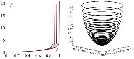
Figure 1: Family of solutions $f(r)$ to (7) with $A_{0}=1,A_{2}=0$ and $A_{1}=i/8\ (i=1\ldots 5)$, producing singular Reeb foliations by rotation about $f$-axis.

Remark 4 (The Bott invariant of transversely holomorphic flows).

Let $Y$ be a nonzero on $M^{2q+1}\setminus\Sigma$ vector field. The flow generated by $Y$ is transversely holomorphic if there is a complex structure $J$ on the $2q$-plane bundle $TM/\langle Y\rangle$ invariant under the flow of $Y$. Assume that $TM/\langle Y\rangle$ is trivial and there is a pair of pointwise linearly independent decomposable $q$-forms $\omega_{1},\omega_{2}$ on $M\setminus\Sigma$ with a common kernel $\ker\omega_{1}\cap\,\ker\omega_{2}$ spanned by $Y$, and such real $2q$-form $\omega_{1}\wedge\omega_{2}$ defines the transverse orientation. If the flow generated by $Y$ is transversely holomorphic then the complex-valued $q$-form $\omega_{c}=\omega_{1}+i\,\omega_{2}$ is formally integrable [10], i.e.,

$$\omega_{c}\wedge d\omega_{c}=0\quad\Longleftrightarrow\quad\bigg{\{}\begin{array}[]{c}\omega_{1}\wedge d\omega_{1}=\omega_{2}\wedge d\omega_{2}\,,\\ \omega_{1}\wedge d\omega_{2}=-\omega_{2}\wedge d\omega_{1}\,.\end{array}$$ (31)

For a complex-valued vector field $T_{c}=T_{1}+i\,T_{2}$ we may assume $\omega_{j}(i\,T_{k})=i\,\omega_{j}(T_{k})$, then

$$\iota_{\,T_{c}}\,\omega_{c}=1\quad\Longleftrightarrow\quad\bigg{\{}\begin{array}[]{c}\iota_{\,T_{1}}\,\omega_{1}+\iota_{\,T_{2}}\,\omega_{2}=1\,,\\ \iota_{\,T_{1}}\,\omega_{2}+\iota_{\,T_{2}}\,\omega_{1}=0\,.\end{array}$$ (32)

If (31) holds, then there is a complex-valued one-form $\eta_{c}=\eta_{1}+i\,\eta_{2}$ such that

$$d\omega_{c}=\omega_{c}\wedge\eta_{c},$$ (33)

moreover, the complex-valued one-form $\eta_{c}$ in (33) can be chosen by

$$\eta_{c}=\iota_{\,T_{c}}\,d\omega_{c}.$$ (34)

Indeed, we have

$$0=\iota_{\,T_{c}}\,(d\omega_{c}\wedge\omega_{c})=\iota_{\,T_{c}}\,d\omega_{c}\wedge\omega_{c}+d\omega_{c}.$$

This and (34) yield (33). For formally integrable $\omega_{c}$, the complex number $\int_{M}\eta_{c}\wedge(d\eta_{c})^{q}$, called the Bott invariant of the flow of $Y$, is independent of choices. For a pair $(\omega_{c},T_{c})$ obeying (32), define

$$\mathrm{gv}(\omega_{c},T_{c}):=\int_{M}\eta_{c}\wedge(d\eta_{c})^{q}.$$

The following fundamental example belongs to R. Bott, see e.g. [2]. Consider a holomorphic vector field $X_{\lambda}=\sum_{j}\lambda_{j}z_{j}\,\partial_{z_{j}}$ on $\mathbb{C}^{q+1}$, where $(z_{0},\ldots,z_{q})$ are standard coordinates and $\lambda_{i}\neq 0$ are complex numbers. Let the convex hull of $\lambda_{0},\ldots,\lambda_{q}$ does not contain the origin. A foliation of $\mathbb{C}^{q+1}$ by orbits of $X$ induces a one-dimensional foliation (flow) ${\cal F}_{\lambda}$ of the unit sphere $S^{2q+1}$. This flow is transversely holomorphic of complex dimension $q$, and $\mathrm{gv}({\cal F}_{\lambda})=(\sum\nolimits_{j}\lambda_{j})^{q+1}/\prod\nolimits_{j}\lambda_{j}$. Hence, the Bott invariant (of the flow above) is non-trivial and admits continuous variations. However, the Godbillon–Vey invariant is rigid under both actual and infinitesimal deformations in the category of transversely holomorphic foliations, see [2]. Notice that for real $q$-forms $\alpha,\beta$, the following equalities hold: $d(\alpha+i\,\beta)=d\alpha+i\,d\beta$,  $({\alpha+i\,\beta})^{\,\centerdot}=\overset{\centerdot}{\alpha}+i\,\overset{\centerdot}{\beta}$,  $(\alpha+i\,\beta)^{\sharp}=\alpha^{\sharp}+i\,\beta^{\sharp}$, and $\iota_{X_{1}+i\,X_{2}}\,\alpha=\iota_{X_{1}}\alpha+i\,\iota_{X_{2}}\alpha$, and Lemma 3 is valid for $\beta_{c}=\beta_{1}+i\,\beta_{2}$ with $\|\beta\|^{2}=\|\beta_{1}\|^{2}+\|\beta_{2}\|^{2}$. Thus, the results of Sections 1, 3 and 4 (Theorems 3 and 4) are valid for complex-valued forms and vector fields.

6 Metric formula for the Godbillon–Vey type invariant

The following Godbillon–Vey type functional is defined for any Riemannian metric on $(M,{\cal D})$:

$$\mathrm{gv}_{\cal D}:g\mapsto-\int_{M}\|H^{\bot}\|\cdot(d\eta)^{q}({\bf T},{\bf B})\,{\rm d}V_{g}.$$ (35)

Here ${\bf B}=B_{1}\wedge\ldots\wedge B_{q}$, where $\{B_{j}\}$ is a local orthonormal frame of ${\cal B}$ such that $({\bf T},N,{\bf B})$ is positive oriented. This $\mathrm{gv}_{\cal D}$ helps us to study the question: What are the best in a sense metrics on a manifold endowed with a distribution ${\cal D}$? Such metrics are proposed to be among critical metrics of the action (35). The $2q$-form $(d\eta)^{q}$ can be expressed on $U$ in terms of extrinsic geometry of ${\cal D}$ and ${\cal D}^{\bot}$.

Theorem 4.

If either ${\cal D}^{\bot}$ or ${\cal B}$ is integrable then the Godbillon–Vey class of $(\omega,{\bf T})$ can be represented by the form $\eta\wedge(d\eta)^{q}$ given by

$$(\eta\wedge(d\eta)^{q})({\bf T},N,{\bf B})=-\|H^{\bot}\|^{q+1}\det(\langle\nabla_{T_{i}}N,B_{j}\rangle-\langle h_{B_{j},N},T_{i}\rangle).$$ (36)

Proof.

If either ${\cal D}^{\bot}$ or ${\cal B}$ is integrable, then – respectively – either $d\eta(T_{i},T_{j})$ or $d\eta(B_{i},B_{j})$ vanish, see Lemma 7 in what follows. Hence,

$$(d\eta)^{q}({\bf T},{\bf B})=\sum\nolimits_{\sigma\in S_{q}}{\rm sign}(\sigma)\cdot d\eta(T_{1},B_{\sigma_{1}})\cdot\ldots\cdot d\eta(T_{q},B_{\sigma_{q}}),$$

where $S_{q}$ is the group of all permutations of the set $\{1,\ldots,q\}$. By Lemma 7 again, (36) holds. ∎

Remark 5.

For $q=1$, the vector field $T$ spans ${\cal D}^{\bot}$ on $(M^{3},g)$. Let $\{T,N,B\}$ be the Frenét frame, and $k$ and $\tau$ the curvature and the torsion of $T$-curves. Then (36) reads as

$$(\eta\wedge d\eta)(T,N,B)=-k^{2}(\tau-h_{B,N}),$$

see [18] and, for integrable ${\cal D}$, [16].

Remark 6.

In [17] we introduced geometric invariants for $n$-tuples, $n\in\mathbb{N}$, of square matrices, or, endomorphisms. Given $n$ such matrices ${\bf A}=(A_{1},\ldots,A_{n})$, consider the polynomial of $n$ variables,

$$P({\bf A})(t_{1},\ldots,t_{n})=\det(\operatorname{id}+t_{1}A_{1}+\ldots+t_{n}A_{n});$$ (37)

the coefficients $\sigma_{\lambda}({\bf A}),\lambda=(\lambda_{1},\ldots,\lambda_{n})\geq 0$ at $t_{1}^{\lambda_{1}}\cdot\ldots\cdot t_{n}^{\lambda_{n}}$ are invariants of our set of matrices. Set $|\lambda|=\lambda_{1}+\ldots+\lambda_{n}$. Taking $t_{1}=\ldots=t_{n}=t$ and comparing the coefficients at $t^{q}$, this yields

$$\det(A_{1}+\ldots+A_{n})=\sum\nolimits_{|\lambda|=q}\sigma_{\lambda}({\bf A}).$$

Formula (36) allows to express the form $\eta\wedge(d\eta)^{q}$ in terms of invariants $\sigma_{\lambda}(A_{1},A_{2})$ of two liner transformations depending on the extrinsic geometry of the almost product structure $({\cal D},{\cal D}^{\bot})$ on $(M,g)$:

$$A_{1}:X\to\nabla^{\top}_{X}N,\quad A_{2}:Y\to\nabla^{\top}_{Y}N=-h(Y,N);$$

hereafter, $\nabla^{\top}$ denotes the connection in the bundle ${\cal D}$ generated by the Levi-Civita connection on $(M,g)$. These maps transform one of the spaces ${\cal B}$ and ${\cal D}^{\bot}$, into another and are represented in positive oriented orthonormal frames by $q$-by-$q$ matrices. With this notation, using (37) with $n=2$, i.e., $\det(A_{1}+A_{2})=\sum\nolimits_{k+l=q}\sigma_{k,l}(A_{1},A_{2})$, (36) reads as

$$(\eta\wedge(d\eta)^{q})({\bf T},N,{\bf B})=-\|H^{\bot}\|^{q+1}\sum\nolimits_{k+l=q}\sigma_{k,l}(A_{1},A_{2}).$$

The integrability tensor ${\cal T}$ of ${\cal D}$ (vanishing for ${\cal D}$ tangent to a foliation) is

$$2\,{\cal T}_{X,Y}=[X,Y]^{\bot}=h_{X,Y}-h_{Y,X},\quad X,Y\in{\cal D}.$$

Let $B_{i}\ (i\leq q)$ be an orthonormal local basis of ${\cal B}$. Set $\operatorname{div}^{\bot}Q=\sum\nolimits_{j}\langle\nabla_{T_{j}}Q,T_{j}\rangle$ for a tensor field $Q$.

Lemma 7.

The 2-form $d\eta$ attains the following values on $U$:

$$(-1)^{q-1}d\eta(N,B_{i})=\|H^{\bot}\|\,\langle\nabla_{N}\,N,B_{i}\rangle-B_{i}(\|H^{\bot}\|)$$

$$=2\langle h_{N,N},{\cal T}_{N,B_{i}}\rangle-2\operatorname{div}^{\bot}{\cal T}_{N,B_{i}}$$

$$+2\sum\nolimits_{j}\big{(}\langle{\cal T}_{(\nabla_{T_{j}}N)^{\top},B_{i}},T_{j}\rangle+\langle h_{B_{j},B_{i}},{\cal T}_{N,B_{j}}\rangle-\langle h_{B_{j},N},{\cal T}_{B_{i},B_{j}}\rangle\big{)}$$ (38)

and

$$(-1)^{q-1}d\eta(T_{i},B_{j})=\|H^{\bot}\|(\langle\nabla_{T_{i}}N,B_{j}\rangle-\langle h_{B_{j},N},T_{i}\rangle),$$

$$(-1)^{q-1}d\eta(B_{i},B_{j})=-\|H^{\bot}\|\cdot\langle[B_{i},B_{j}],N\rangle,$$

$$(-1)^{q-1}d\eta(T_{i},T_{j})=-\|H^{\bot}\|\cdot\langle[T_{i},T_{j}],N\rangle,$$

$$(-1)^{q-1}d\eta(T_{i},N)=T_{i}(\|H^{\bot}\|)-\|H^{\bot}\|\langle h_{N,N},T_{i}\rangle.$$ (39)

Proof.

Using (5), one gets the first equality of (7),

$$d\eta(N,B_{i}) = N(\eta(B_{i}))-B_{i}(\eta(N))-\eta([N,B_{i}])$$

$$= (-1)^{q-1}\big{(}\|H^{\bot}\|\,\langle\nabla_{N}N,B_{i}\rangle-B_{i}(\|H^{\bot}\|)\big{)}.$$

Differentiating $\langle[N,B_{i}],T_{j}\rangle$ in the $T_{j}$-direction, after a lengthy calculation using symmetries of the curvature tensor $R$, yields

$$\sum\nolimits_{j}T_{j}\,(\langle[N,B_{i}],T_{j})\rangle=\langle[N,B_{i}],H^{\bot}\rangle+\sum\nolimits_{j}\langle\nabla_{N}\nabla_{T_{j}}\,B_{i}$$

$$+\nabla_{[T_{j},N]}B_{i}+R_{T_{j},N}B_{i}-\nabla_{B_{i}}\nabla_{T_{j}}\,N-\nabla_{[T_{j},B_{i}]}\,N-R_{T_{j},B_{i}}N,\ T_{j}\rangle$$

$$=\|H^{\bot}\|\,\langle[N,B_{i}],N\rangle+\sum\nolimits_{j}\langle-\nabla_{N}(\tau_{ji}N)+\nabla_{A_{j}N+\sum\nolimits_{l}(\tau_{jl}B_{l}-k_{jl}T_{l})}B_{i}$$

$$+\nabla_{B_{i}}(\sum\nolimits_{l}k_{jl}T_{l})-\nabla_{B_{i}}(\sum\nolimits_{l}\tau_{jl}B_{l})-\nabla_{A_{j}B_{i}-\tau_{ji}N}\,N-R_{N,B_{i}}T_{j},\ T_{j}\rangle$$

$$=B_{i}(\|H^{\bot}\|)-\|H^{\bot}\|\,\langle\nabla_{N}N,B_{i}\rangle+2\langle h_{N,N},{\cal T}_{N,B_{i}}\rangle$$

$$+\,2\sum\nolimits_{j}\big{(}\langle{\cal T}_{(\nabla_{T_{j}}N)^{\top},B_{i}},T_{j}\rangle+\langle h_{B_{j},B_{i}},{\cal T}_{N,B_{j}}\rangle-\langle h_{B_{j},N},{\cal T}_{B_{i},B_{j}}\rangle\big{)}.$$

Here we used $A_{j}X:=-(\nabla_{X}T_{j})^{\top}\ (X\in{\cal D})$ and Frenét type formulas for ${T}_{i}$-derivatives:

$$\nabla_{T_{i}}\,T_{j} = -k_{ij}N+\sum\nolimits_{k}s_{ijk}B_{k},\quad\nabla_{T_{i}}\,N=-k_{ij}T_{j}+\sum\nolimits_{j}\tau_{ij}B_{j},$$

$$\nabla_{T_{i}}\,B_{j} = -\tau_{ij}N-\sum\nolimits_{k}s_{ikj}B_{k}$$

with certain functions $k_{ij}$ and $s_{ikj}$. Note that $\sum_{i}k_{ii}=\langle H^{\bot},N\rangle$. From this, the definition of ${\cal T}$ and

$$2\operatorname{div}^{\bot}{\cal T}_{N,B_{i}}=2\sum\nolimits_{j}\langle\nabla_{T_{j}}({\cal T}_{N,B_{i}}),T_{j}\rangle=\sum\nolimits_{j}T_{j}(\langle[N,B_{i}]^{\bot},T_{j})\rangle$$

we deduce the second equality of (7). Next,

$$d\eta(T_{i},B_{j})=T_{i}(\eta(B_{j}))-B_{j}(\eta(T_{i}))-\eta([T_{i},B_{j}])=(-1)^{q}\|H^{\bot}\|\,\langle[T_{i},B_{j}],N\rangle,$$

from which (7)₁ follows. The proofs of (7)_2,3,4 are also straightforward. ∎

Lemma 8.

Let ${\cal D}=\ker\omega$ be a codimension $q$ distribution on $M^{2q+1}$ and $g\in{\rm Riem}(M,{\cal D},{\bf T})$.

$(i)$ If $T_{i}(t)=C^{j}_{i}(t)\,T_{j}$ and $\omega(t)=\det C(t)^{-1}\omega$ for some $C(t):M\to GL(q,\mathbb{R})$ such that $C(0):M\to{\rm id}_{q}$, then

$$(\eta\wedge(d\eta)^{q})^{\,\centerdot} = (q+1)\sum\nolimits_{i}(-1)^{i}T_{i}(\operatorname{Tr}\dot{C})\,(d\eta)^{q}(\widehat{\bf T}_{i},N,{\bf B})\,{\rm d}V_{g}$$ (40)

$$+\,d(\dot{\eta}\wedge\eta\wedge(d\eta)^{q-1}+(q+1)\,(\operatorname{Tr}\dot{C})\,(d\eta)^{q}).$$

$(ii)$ If $T_{i}(t)=T_{i}+X_{i}(t)$ for $X_{i}(t)\in\mathfrak{X}_{\cal D}\ (|t|<\varepsilon)$ such that $X_{i}(0)=0$ and $\omega(t)=\omega$, then

$$({\eta\wedge(d\eta)^{q}})^{\,\centerdot}=(q+1)\big{[}d\omega(\dot{\bf X},N)\,(d\eta)^{q}({\bf B},{\bf T})$$

$$+\sum\nolimits_{i}(-1)^{i-1}d\omega(\dot{\bf X},T_{i})\,(d\eta)^{q}(\widehat{\bf T}_{i},N,{\bf B})$$ (41)

$$+\sum\nolimits_{k}(-1)^{q+k}d\omega(\dot{\bf X},B_{k})\,(d\eta)^{q}({\bf T},N,\widehat{\bf B}_{k})\big{]}\,{\rm d}V_{g}-d(\eta\wedge(d\eta)^{q-1}\wedge\iota_{\,\dot{\bf X}}\,d\omega).$$

Proof.

Notice that in both cases, (i) and (ii), (8) holds.

(i) We have $\dot{T}_{i}=\dot{C}^{j}_{i}\,T_{j}$ and $\dot{\omega}=-\dot{c}\,\omega$, where $c(t)=\det C(t)$. By Jacobi’s formula, that expresses the derivative of $\det C$ in terms of the adjunct of $C$ and the derivative of $C$, and conditions, we have $\dot{c}=\operatorname{Tr}\dot{C}$. Since (9) and $\iota_{\,N}\,\omega=\iota_{\,B_{k}}\,\omega=0$, the following equalities provide (40):

$$({\eta\wedge(d\eta)^{q}})^{\,\centerdot} = (q+1)\sum\nolimits_{i}(-1)^{i}T_{i}(\dot{c})\,\iota_{\,\widehat{\bf T}_{i}}\omega\wedge(d\eta)^{q}$$

$$+ d\big{(}\eta\wedge\dot{\eta}\wedge(d\eta)^{q}-(q+1)\,\dot{c}\,(d\eta)^{q}\big{)},$$

$$(\iota_{\,\widehat{\bf T}_{i}}\omega\wedge(d\eta)^{q})({\bf T},N,{\bf B}) = \omega({\bf T})\,(d\eta)^{q}(\widehat{\bf T}_{i},N,{\bf B})=(d\eta)^{q}(\widehat{\bf T}_{i},N,{\bf B}).$$

(ii) We have $\dot{\bf X}=\sum\nolimits_{i}(-1)^{i-1}\dot{X}_{i}\wedge\widehat{\bf T}_{i}$, $\dot{X}_{i}=\dot{T}_{i}$ and $\dot{\omega}=0$. Since $\dot{\eta}=\iota_{\,\dot{\bf X}}\,d\omega$, see (9), we get

$$({\eta\wedge(d\eta)^{q}})^{\,\centerdot}=(q+1)\,\iota_{\,\dot{\bf X}}\,d\omega\wedge(d\eta)^{q}-d(\eta\wedge(d\eta)^{q-1}\wedge\iota_{\,\dot{\bf X}}\,d\omega).$$

Then we obtain

$$\iota_{\,\dot{\bf X}}\,d\omega\wedge(d\eta)^{q}({\bf T},N,{\bf B}) = d\omega(\dot{\bf X},N)\,(d\eta)^{q}({\bf B},{\bf T})$$

$$+ \sum\nolimits_{i}(-1)^{i-1}d\omega(\dot{\bf X},T_{i})\,(d\eta)^{q}(\widehat{\bf T}_{i},N,{\bf B})$$

$$+ \sum\nolimits_{k}(-1)^{q+k}d\omega(\dot{\bf X},B_{k})\,(d\eta)^{q}({\bf T},N,\widehat{\bf B}_{k}),$$

and (8) follows from the above. ∎

Remark 7.

If the distribution ${\cal B}$ is integrable then the factor in the right hand side of (40), see also (8), is

$$(d\eta)^{q}(\widehat{\bf T}_{i},N,{\bf B})=\sum\nolimits_{j}(-1)^{j}\,d\eta(N,B_{j})\,(d\eta)^{q-1}(\widehat{\bf T}_{i},\widehat{\bf B}_{j}),$$ (42)

and if, in addition, the distribution ${\cal D}^{\bot}$ is integrable then the factor in the right hand side of (42) is

$$(d\eta)^{q-1}(\widehat{\bf T}_{i},\widehat{\bf B}_{j}){=}\sum\nolimits_{\sigma\in S^{j}_{q-1}}\!\!{\rm sign}(\sigma)\,d\eta((\widehat{\bf T}_{i})_{1},B_{\sigma_{1}})\cdot\ldots\cdot d\eta((\widehat{\bf T}_{i})_{q-1},B_{\sigma_{q-1}}),$$

where $S^{j}_{q-1}$ denotes the group of all permutations of the set $\{1,\ldots,\hat{j},\ldots,q\}$.

7 Variations of metric

Let $g=g_{0}\in{\rm Riem}(M^{2q+1},{\cal D},{\bf T})$ and $g_{t}\ (|t|<\varepsilon)$ be an arbitrary one-parameter family of metrics on $(M,{\cal D})$. Note that the symmetric $(0,2)$-tensor $\dot{g}$ has only $(q+1)(2q+1)$ independent components.

A family $g_{t}$ preserving a metric on ${\cal D}$ is called $g^{\pitchfork}$-variation: its tensor $\dot{g}$ has $\frac{3}{2}\,q(q+1)$ nonzero components $\{\dot{g}_{\,T_{i},T_{j}}=\dot{g}_{\,T_{j},T_{i}},\dot{g}_{\,T_{i},N},\dot{g}_{\,T_{i},B_{k}}\}$. Variations $g_{t}$, with only $\frac{1}{2}\,q(q+1)$ nonzero components $\{\dot{g}_{B_{i},B_{j}}=\dot{g}_{B_{j},B_{i}}\}$ preserve both ${\cal D}$ and ${\cal D}^{\bot}$, and thus produce trivial Euler-Lagrange equations for (35). If ${\cal D}$ is integrable then (35) is constant, hence Euler-Lagrange equations are trivial.

An arbitrary $g^{\pitchfork}$-variation of a Riemannian metric $g$ can be decomposed into two cases:

(i) $g$ varies along ${\cal D}^{\bot}$ only; (ii) variations preserve $g$ on ${\cal D}$ and $\{T_{i}\}$ but disturb their orthogonality.

Thus, we can divide all nonzero components of $\dot{g}$ into two sets: $\{\dot{g}_{\,T_{i},T_{j}}\}$ and $\{\dot{g}_{\,T_{i},N},\dot{g}_{\,T_{i},B_{k}}\}$.

Theorem 5.

Let $T_{i}\ (1\leq i\leq q)$ be linear independent vector fields transverse to a codimension $q$ distribution ${\cal D}=\ker\omega$ on $M^{2q+1}\setminus\Sigma$. Then $g\in{\rm Riem}(M,{\cal D},{\bf T})$ is critical for $\mathrm{gv}_{\cal D}$ in (35) with respect to all variations $g_{t}$ obeying (8) and

$$\int_{M}\|(\operatorname{Tr}\dot{B})\sum\nolimits_{i}(-1)^{i}(d\eta)^{q}(\widehat{\bf T}_{i},N,{\bf B})\cdot T_{i}$$ (43b)

$$+\,\dot{\eta}\wedge\eta\wedge(d\eta)^{q-1}\!+(q+1)(\operatorname{Tr}\dot{C})\,(d\eta)^{q}\|^{p}\,{\rm d}V_{g}<\infty,$$

$$\int_{M}\|\iota_{\,\dot{\bf X}}\,d\omega\wedge\eta\wedge(d\eta)^{q-1}\|^{p}\,{\rm d}V_{g}<\infty$$

for some $p$ such that $(k-1)(p-1)\geq 1$, if and only the following $q^{2}+q+1$ equations hold on $U$:

$$\hskip-22.76219pt\operatorname{div}\big{(}\sum\nolimits_{i}(-1)^{i}(d\eta)^{q}(\widehat{\bf T}_{i},N,{\bf B})\cdot T_{i}\big{)}=0,$$ (44a)

$$\hskip-22.76219pt(d\eta)^{q}(\widehat{\bf T}_{i},N,{\bf B})\cdot\|H^{\bot}\|=-\sum\nolimits_{k}(-1)^{k}(d\eta)^{q}({\bf T},N,\widehat{\bf B}_{k})\,d\omega(N,\widehat{\bf T}_{i},B_{k}),$$ (44b)

$$\hskip-25.60747pt(d\eta)^{q}({\bf B},{\bf T})\,d\omega(B_{j},\widehat{\bf T}_{i},N){=}-\!\!\sum\limits_{k}\!(-1)^{q+k}(d\eta)^{q}({\bf T},N,\widehat{\bf B}_{k})d\omega(B_{j},\widehat{\bf T}_{i},B_{k}).$$ (44c)

For integrable ${\cal D}$, equations $($44a-c$)$ reduce to the expected trivial equalities.

Proof.

According to Lemma 8, one should consider only two cases.

Case 1. Let $\dot{T}_{i}=\dot{C}^{j}_{i}\,T_{j}$ and $\dot{\omega}=-\dot{c}\,\omega$, where $c(t)=\det C(t)$. Differentiating $g_{t}(T_{i}(t),T_{j}(t))=\delta_{ij}$ at $t=0$ we obtain $\dot{g}_{ij}=-\dot{C}^{j}_{i}-\dot{C}^{i}_{j}$. Hence, $\sum\nolimits_{i}\dot{g}_{\,T_{i},T_{i}}=-2\operatorname{Tr}\dot{C}$. By Lemma 8(i), and using

$$\operatorname{div}(Q_{i}\operatorname{Tr}\dot{C}\cdot T_{i})=(\operatorname{Tr}\dot{C})\operatorname{div}(Q_{i}\cdot T_{i})+Q_{i}T_{i}(\operatorname{Tr}\dot{C})$$

with $Q_{i}=(-1)^{i}(d\eta)^{q}(\widehat{\bf T}_{i},N,{\bf B})\,{\rm d}V_{g}$, we have

$$({\eta\wedge(d\eta)^{q}})^{\,\centerdot}=-(q+1)(\operatorname{Tr}\dot{C})\operatorname{div}\big{(}\sum\nolimits_{i}(-1)^{i}(d\eta)^{q}(\widehat{\bf T}_{i},N,{\bf B})\cdot T_{i}\big{)}\,{\rm d}V_{g}$$

$$+\,\operatorname{div}((\operatorname{Tr}\dot{C})\sum\nolimits_{i}(-1)^{i}(d\eta)^{q}(\widehat{\bf T}_{i},N,{\bf B})\cdot T_{i})\,{\rm d}V_{g}$$

$$+d\big{(}\dot{\eta}\wedge\eta\wedge(d\eta)^{q-1}+(q+1)\,(\operatorname{Tr}\dot{C})\,(d\eta)^{q}\big{)}.$$

By Stokes theorem and (43b), the Euler-Lagrange equations read as (44a).

Case 2. Now, let $T_{i}(t)=T_{i}+X_{i}(t)$ be the orthonormal frame of ${\cal D}_{t}^{\bot}$ with respect to $g_{t}$ for some vector fields $X_{i}(t)\in\mathfrak{X}_{\cal D}$ with $X_{i}(0)=0$. Differentiating $g_{t}(T_{i}+X_{i}(t),N)=0$ at $t=0$ we obtain

$$\langle\dot{X}_{i},N\rangle=-\dot{g}_{\,T_{i},N}.$$

Similarly, $\langle\dot{X}_{i},B_{j}\rangle=-\dot{g}_{\,T_{i},B_{j}}$. Hence, $\dot{X}_{i}=-\dot{g}_{\,T_{i},N}N-\sum\nolimits_{j}\dot{g}_{\,T_{i},B_{j}}B_{j}$, and

$$d\omega(\dot{\bf X},T_{i}) = \sum\nolimits_{j}(-1)^{j}\big{[}d\omega(N,\widehat{\bf X}_{j},T_{i})\,\dot{g}_{\,T_{j},N}+\sum\nolimits_{k}d\omega(B_{k},\widehat{\bf X}_{j},T_{i})\,\dot{g}_{\,T_{i},B_{k}}\big{]}$$

$$= (-1)^{i}\big{[}d\omega(N,\widehat{\bf T}_{i},T_{i})\,\dot{g}_{\,T_{i},N}+\sum\nolimits_{k}d\omega(B_{k},\widehat{\bf T}_{i},T_{i})\,\dot{g}_{\,T_{i},B_{k}}\big{]}$$

$$= (-1)^{q}\big{[}d\omega(N,{\bf T})\,\dot{g}_{\,T_{i},N}+\sum\nolimits_{k}d\omega(B_{k},{\bf T})\,\dot{g}_{\,T_{i},B_{k}}\big{]}$$

$$= (-1)^{q-1}\,\|H^{\bot}\|\,\dot{g}_{\,T_{i},N},$$

$$d\omega(\dot{\bf X},N) = -\sum\nolimits_{k,i}(-1)^{i-1}d\omega(B_{k},\widehat{\bf T}_{i},N)\,\dot{g}_{\,T_{i},B_{k}},$$

$$d\omega(\dot{\bf X},B_{k}) = -\!\sum\nolimits_{i}(-1)^{i-1}\big{(}d\omega(N,\widehat{\bf T}_{i},B_{k})\,\dot{g}_{\,T_{i},N}{+}\!\sum\nolimits_{j}d\omega(B_{j},\widehat{\bf T}_{i},B_{k})\,\dot{g}_{\,T_{i},B_{j}}\big{)}.$$

Here we used $\dot{\bf X}=\sum\nolimits_{j}(-1)^{j-1}\dot{X}_{i}\wedge\widehat{\bf T}_{i}$ and $d\omega(N,{\bf T})=-\|H^{\bot}\|$. Then, by Lemma 8(ii), we have

$$\hskip 8.53581pt({\eta\wedge(d\eta)^{q}})^{\,\centerdot}=(q+1)\big{(}-\sum\nolimits_{i,j}(-1)^{i-1}(d\eta)^{q}({\bf B},{\bf T})\,d\omega(B_{j},\widehat{\bf T}_{i},N)\,\dot{g}_{\,T_{i},B_{j}}$$

$$+\sum\nolimits_{i}(-1)^{q+i-2}\|H^{\bot}\|\,(d\eta)^{q}(\widehat{\bf T}_{i},N,{\bf B})\,\dot{g}_{\,T_{i},N}$$

$$-\sum\nolimits_{k}(-1)^{q+k+i-1}\big{(}d\omega(N,\widehat{\bf T}_{i},B_{k})\,\dot{g}_{\,T_{i},N}$$

$$+\sum\nolimits_{j}d\omega(B_{j},\widehat{\bf T}_{i},B_{k})\,\dot{g}_{\,T_{i},B_{j}}\big{)}(d\eta)^{q}({\bf T},N,\widehat{\bf B}_{k})\big{)}\,{\rm d}V_{g}-d(\eta\wedge(d\eta)^{q-1}\!\wedge\iota_{\,\dot{\bf X}}\,d\omega).$$

By Stokes theorem and (43b), the vanishing of $\dot{g}_{\,T_{i},N},\dot{g}_{\,T_{i},B_{k}}$ components provides (44b,c). ∎

Remark 8.

For $q=1$, (44a-c) reduce to the following system of equations on $U$, see [18, Theorem 4.2]:

$$\operatorname{div}(\operatorname{div}({\mathcal{T}}_{N,B}\cdot T)\cdot T) = 0,$$ (45a)

$$\operatorname{div}({\mathcal{T}}_{N,B}\cdot T)-(T(\log k)-h_{N,N}){\mathcal{T}}_{N,B} = 0,$$ (45b)

$$(\tau-h_{B,N})\,{\mathcal{T}}_{N,B} = 0.$$ (45c)

Corollary 5.

Let $g\in{\rm Riem}(M,{\cal D},{\bf T})$ and either $(d\eta)^{q}=0$ or the normal distribution ${\cal D}^{\bot}$ be harmonic. Then $g$ is a critical point for $\mathrm{gv}_{\cal D}$ with respect to all variations of metric obeying (8) and (43b,b).

Proof.

If $(d\eta)^{q}=0$ then (44a-c) hold, hence $g$ is critical. If $H^{\bot}=0$, then $\eta=0$, $d\eta=0$, see (5), and (44a-c) and (43b,b) are satisfied trivially. ∎

References

• [1] T. Asuke, Transverse projective structures of foliations and infinitesimal derivatives of the Godbillon–Vey class, Int. J. of Math. 26, No. 4, 2015 (29 pages).
• [2] T. Asuke, Godbillon–Vey class of transversely holomorphic foliations, MSJ Memories, 24, 2010.
• [3] D. Blair, Riemannian geometry of contact and symplectic manifolds, Springer, 2010.
• [4] F. Brito and P. Walczak, On the energy of unit vector fields with isolated singularities, Ann. Polon. Math. 73 (2000), 269–274.
• [5] A. Candel and L. Conlon, Foliations I and II, Amer. Math. Soc. 2000 and 2003.
• [6] B.Y. Chen, Geometry of submanifolds and its applications, Science Univ. of Tokyo, 1981.
• [7] A. Echeverría-Enríquez, M.C. Munoz-Lecanda and N. Roman-Roy, Multivector fields and connections: setting Lagrangian equations in field theories, J. Math. Phys. 39 (9) (1998) 4578–4603.
• [8] M. Forger, C. Paufler and H. Römer, The Poisson bracket for Poisson forms in multisymplectic field theory, Rev. Math. Phys. 15 (2003), no. 7, 705–743.
• [9] P. Foulon and B. Hasselblatt, Godbillon–Vey invariants for maximal isotropic $C^{2}$-foliations, Adv. Studies in Pure Mathematics, 72 (2017), 349–366.
• [10] H. Geiges and J.G. Pérez, Transversely holomorphic flows and contact circles on spherical 3-manifolds, Enseign. Math. 62 (2016), no. 3–4, 527–567.
• [11] E. Ghys, R. Langevin and P. Walczak, Entropie géométrique des feuilletages, Acta Math. 160 (1988), 105–142.
• [12] H. Gluck, Dynamical behavior of geodesic fields, 190–215. In “Global Theory of Dynamical Systems”, LNM, vol. 819, Springer, 1980.
• [13] C. Godbillon and J. Vey, Un invariant des feuilletages de codimension 1, C. R. Acad. Sci. Paris, Comptes Rendus, sér. A, 273 (1971), 92–95.
• [14] S. Hurder, Dynamics of the Godbillon–Vey class: a history and survey, in Foliations: Geometry and Dynamics (Warsaw 2000), World. Sci. Publ. 2002, 29–60.
• [15] S. Hurder, Problem set, in Foliations 2005, World Sci. Publ. 2006, 441–475.
• [16] B.L. Reinhart and J.W. Wood, A metric formula for the Godbillon–Vey invariant for foliations, Proc. Amer. Math. Soc., 38, No. 2 (1973), 427–430.
• [17] V. Rovenski and P. Walczak, Integral formulae on foliated symmetric spaces, Math. Ann. 352(1), (2012), 223–237.
• [18] V. Rovenski and P. Walczak, Variations of the Godbillon–Vey invariant of foliated 3-manifolds, Complex Analysis and Operator Theory, 2018, https://doi.org/10.1007/s11785-018-0871-9.
• [19] D. Sullivan, A homological characterization of foliations consisting of minimal surfaces, Comm. Math. Helv. 54 (1979), 218–223.
• [20] I. Tamura, Topology of Foliations, Iwananmi Shoten, 1076 (English transl.: AMS, 1992).
• [21] P. Walczak, Dynamics of Foliations, Groups and Pseudogroups, Birkhäuser, 2004.
• [22] P. Walczak, Tautness and the Godbillon–Vey class of foliations. In Proc. “Foliations 2012”, 205–213, World Sci. Publ., 2013.
• [23] P. Walczak, Integral formulae for foliations with singularities, Coll. Math. 150, (2017), 141–148.
• [24] G.M. Webb, A. Prasad, S.C. Anco and Q. Hu, Godbillon-Vey helicity and magnetic helicity in Magnetohydrodynamics, arXiv: 1909.0729 [astro-ph.SR], 2019, 42 pp.