Energy Stability of Explicit Runge-Kutta Methods for Non-autonomous or Nonlinear Problems

Abstract

Many important initial value problems have the property that energy is non-increasing in time. Energy stable methods, also referred to as strongly stable methods, guarantee the same property discretely. We investigate requirements for conditional energy stability of explicit Runge-Kutta methods for nonlinear or non-autonomous problems. We provide both necessary and sufficient conditions for energy stability over these classes of problems. Examples of conditionally energy stable schemes are constructed and an example is given in which unconditional energy stability is obtained with an explicit scheme.

Keywords. Runge-Kutta methods, energy stability, strong stability, monotonicity, semiboundedness, dissipation, conservation

Mathematics Subject Classification (2010). 65L06, 65L20, 65M12, 65M20

1 Introduction

Ever since the construction of numerical methods for ordinary and (time-dependent) partial differential equations (ODEs and PDEs, respectively), their stability has been an important and active topic of research. Monotonicity, meaning that the norm of the solution is bounded by its initial value, is a particularly exacting stability property. For equations, such as parabolic PDEs, that contain a significant amount of dissipation, any reasonable numerical method will typically preserve monotonicity under an appropriate time step restriction. In contrast, for non-dissipative problems such as hyperbolic PDEs (and their slightly dissipative semidiscretizations), common time discretizations may not preserve monotonicity under any finite step size.

For nonlinear problems, such stability properties of numerical methods are interesting and relevant in practice, e.g. for computational fluid dynamics [39]. But important applications are not restricted to such nonlinear problems. Linear problems with time-dependent operators occur for example if the passive transport of a tracer in a fluid is considered. Other examples occur in the field of plasma physics when a hybrid method is used and the motion of macro-particles is coupled in an operator splitting approach to the evolution of the magnetic field, which is determind as the solution of a linear hyperbolic PDE with time-dependent coefficients [20, 37]. Such problems are not only much more complex in terms of stability (as outlined in this article) but also in terms of the asymptotic error growth [26].

The energy method is an effective tool to get stability estimates, e.g. for hyperbolic PDEs [21, 13]. Using summation by parts operators [45, 9], these can be transferred efficiently to the semidiscrete level for many different kinds of schemes [22, 23, 11, 36]. However, applying the same approach in time yields implicit methods [24, 2, 29, 34, 10]. Classical nonlinearly stable methods, such as algebraically stable Runge-Kutta methods, are also implicit. For hyperbolic problems, such implicit methods are usually less efficient than explicit ones. It is possible to obtain conditional energy stability with explicit methods by using modifications that go outside the class of Runge-Kutta methods; e.g. projection methods [14, 6, 5] and relaxation Runge-Kutta schemes [19, 38, 33, 30]. Another possibility, studied in particular in the context of hyperbolic PDEs, is to add artificial dissipation, spectral viscosity, or filtering [12, 25, 42]. If these modifications are implemented after a full Ruge-Kutta step, they belong to the same general class of projection methods as relaxation and orthogonal projection schemes.

Before trying to modify existing algorithms to prove stability results, it is of course interesting to know whether these modifications are really necessary to get stability or only for a proof thereof. Additionally, modifications of explicit methods can make the algorithm more complicated and some versions can even destroy other desired properties while trying to impose stability [25, 32]. Hence, it is interesting to know what can be achieved within the class of explicit Runge-Kutta methods without modifications. In this setting, results have been obtained for problems that include a certain amount of dissipation [8, 17]. Recently this topic has again attracted the interest of researchers and several results (using the term strong stability) for linear, time-independent operators have been discovered [35, 43, 44]. Nonlinear problems have been investigated in [28], where many non-existence results for energy stable and strong stability preserving (SSP) methods of order two and greater have been proved. A first order accurate energy stable SSP method for autonomous problems has also been discovered therein.

This article extends these previous works considerably by studying both time-dependent linear and autonomous nonlinear problems. After introducing the notation and reviewing some basic results in Section 2, the focus lies on time-dependent linear operators in Section 3. The main result, Theorem 3.2, gives necessary conditions for conditional energy stability in this setting. These conditions are not satisfied by any known Runge-Kutta scheme we are aware of. However, an example of a scheme fulfilling these necessary conditions is given, and is proved to be energy stable for a restricted class of relevant problems (Proposition 3.7).

Next, autonomous nonlinear problems are studied in Section 4. The necessary conditions in this setting are, perhaps surprisingly, weaker than in the non-autonomous linear case. These conditions are based on an expansion of the change of energy (26), which is also used to study sufficient conditions for energy stability. Based thereon, we give a procedure for developing energy stable schemes, and give examples of schemes of second and third order (Theorem 4.12 and Example 4.15).

While most of the paper is devoted to the guarantee of stability over a whole class of semibounded problems, in Section 5 we ask whether an explicit Runge-Kutta method can be unconditionally energy stable for some specific problem. We show that this is impossible if the problem is linear, but – surprisingly – we give an example of unconditional stability for a nonlinear problem. Finally, in Section 6, the results are summed up, open questions are discussed, and directions of future research are outlined.

2 Energy Evolution by Runge-Kutta Methods

Consider a time-dependent initial value problem

$$\dfrac{\operatorname{d\!}{}}{\operatorname{d\!}{t}}u(t) =f(t,u(t)), t\in(0,T),$$ (1)

$$u(0) =u_{0},$$

in a real Hilbert space $\mathcal{H}$ with inner product $\left\langle{\cdot,\,\cdot}\right\rangle$, inducing the norm $\mathinner{\!\left\lVert\cdot\right\rVert}$. We refer to $\mathinner{\!\left\lVert\cdot\right\rVert}^{2}$ as the energy.

2.1 Energy Stability

For a smooth solution of (1), the time derivative of the energy is

$$\dfrac{\operatorname{d\!}{}}{\operatorname{d\!}{t}}\mathinner{\!\left\lVert u(t)\right\rVert}^{2}=2\left\langle{u(t),\,\dfrac{\operatorname{d\!}{}}{\operatorname{d\!}{t}}u(t)}\right\rangle=2\left\langle{u(t),\,f(t,u(t))}\right\rangle.$$ (2)

Definition 2.1.

The right hand side $f\colon[0,T]\times\mathcal{H}\to\mathcal{H}$ of (1) is semibounded, if

$$\forall u\in\mathcal{H},t\in[0,T]\colon\quad\left\langle{u,\,f(t,u)}\right\rangle\leq 0.$$ (3)

If $f$ is semibounded, the ODE (1) will sometimes also be called semibounded.

Remark 2.2.

The results in this work extend to complex Hilbert spaces if one assumes that the real part of the inner product $\left\langle{u,\,f(t,u)}\right\rangle$ is non-positive.

Thus, the energy of any smooth solution of (1) is bounded by its initial value if $f$ is semibounded. However, an approximate solution obtained by a numerical method does not necessarily satisfy this inequality. For example, applying one step of the explicit Euler method to (1) yields the new value $u_{+}=u_{0}+\Delta tf(0,u_{0})$, satisfying

$$\mathinner{\!\left\lVert u_{+}\right\rVert}^{2}=\mathinner{\!\left\lVert u_{0}+\Delta tf(0,u_{0})\right\rVert}^{2}=\mathinner{\!\left\lVert u_{0}\right\rVert}^{2}+\underbrace{2\Delta t\left\langle{u_{0},\,f(0,u_{0})}\right\rangle}_{\leq 0}+\underbrace{\Delta t^{2}\mathinner{\!\left\lVert f(0,u_{0})\right\rVert}^{2}}_{\geq 0}.$$ (4)

Thus, for a general semibounded $f$, the norm of the numerical solution can increase during one time step, e.g. if $\left\langle{u_{0},\,f(0,u_{0})}\right\rangle=0$. In particular, this happens if $f(t,u)=L(t)u$, where $L(t)\neq 0$ is a skew-symmetric operator.

Definition 2.3.

A one-step numerical scheme for approximating the solution of (1) is conditionally energy stable with respect to a class ${\mathcal{F}}$ of semibounded problems if for each $f\in{\mathcal{F}}$ there exists $\Delta t_{\mathrm{max}}>0$ such that $\mathinner{\!\left\lVert u_{+}\right\rVert}^{2}\leq\mathinner{\!\left\lVert u_{0}\right\rVert}^{2}$ for all $0<\Delta t\leq\Delta t_{\mathrm{max}}$.

Here $\Delta t_{\mathrm{max}}$ may depend on $f$, $u_{0}$, and the method itself. In the following we will consider the classes ${\mathcal{F}}$ of linear non-autonomous and nonlinear autonomous problems. We will often omit the word conditional for brevity.

2.2 Runge-Kutta Methods

A general (explicit or implicit) Runge-Kutta method with $s$ stages can be described by its Butcher tableau [15, 4]

$$\begin{array}[]{c | c}c&A\\ \hline\cr&b\end{array}$$ (5)

where $A\in\mathbb{R}^{s\times s}$ and $b,c\in\mathbb{R}^{s}$. For (1), a step from $u_{0}$ to $u_{+}$ is given by

$$u_{i}=u_{0}+\Delta t\sum_{j=1}^{s}a_{ij}\,f(c_{j}\Delta t,u_{j}),\qquad u_{+}=u_{0}+\Delta t\sum_{i=1}^{s}b_{i}\,f(c_{i}\Delta t,u_{i}).$$ (6)

Here, $u_{i}$ are the stage values of the Runge-Kutta method. It is also possible to express the method via the slopes $k_{i}=f(c_{i}\Delta t,u_{i})$.

Using the stage values $u_{i}$ as in (6), the change in energy can be written after some simplifications using the symmetry of the inner product as [4, equation (357e)]

$$\mathinner{\!\left\lVert u_{+}\right\rVert}^{2}-\mathinner{\!\left\lVert u_{0}\right\rVert}^{2}=2\Delta t\sum_{i=1}^{s}b_{i}\left\langle{u_{i},\,f(c_{i}\Delta t,u_{i})}\right\rangle\\ +(\Delta t)^{2}\left[\sum_{i,j=1}^{s}\left(b_{i}b_{j}-b_{i}\,a_{ij}-b_{j}a_{ji}\right)\left\langle{f(c_{i}\Delta t,u_{i}),\,f(c_{j}\Delta t,u_{j})}\right\rangle\right].$$ (7)

The first term on the right hand side is consistent with $\int_{t_{0}}^{t_{0}+\Delta t}2\left\langle{u(t),\,f(t,u(t))}\right\rangle\operatorname{d\!}t$, if the Runge-Kutta method is consistent, i.e. $\sum_{i=1}^{s}b_{i}=1$. Semiboundedness of $f$ implies that this term is non-positive if all $b_{i}$ are non-negative.

We recall the classical property of algebraic stability, which guarantees energy stability for semibounded operators; cf. [4, section 357] and references cited therein.

Definition 2.4.

A Runge-Kutta method is algebraically stable if $b_{i}\geq 0$ for all $i$ and the matrix with entries $(b_{i}b_{j}-b_{i}\,a_{ij}-b_{j}a_{ji})_{i,j}$ is negative semidefinite.

Comparison with (7) shows that algebraically stable Runge-Kutta methods are energy stable for any time step size $\Delta t>0$, cf. [4, section 357] and references cited therein. While there are Runge-Kutta methods with these nice stability properties such as Gauß, Radau IA/IIA or Lobatto IIIC schemes, these are necessarily implicit.

For linear and semibounded problems (1) with constant coefficients, several results concerning the conditional energy stability of explicit Runge-Kutta methods have been achieved [46, 35, 43, 44] (note that the term conditional energy stability herein is precisely what is meant by strong stability in the latter works). Typically, conditional energy stability can be guaranteed for problems $f(t,u)=Lu$ in this class under a time step restriction of the form $\Delta t\leq C\mathinner{\!\left\lVert L\right\rVert}^{-1}$, corresponding to a classical CFL criterion for discretizations of hyperbolic conservation laws [46, 35, 43, 44]. Similar results have been obtained for some first order accurate schemes and autonomous semibounded nonlinear problems [28]. In the latter setting, the maximal time step is proportional to the inverse of the Lipschitz constant of the nonlinear right-hand side $f$ of the ODE.

3 Non-autonomous Linear Operators

In this section, the special case of non-autonomous linear operators is studied. Hence,

$$\dfrac{\operatorname{d\!}{}}{\operatorname{d\!}{t}}u(t) =L(t)u(t), t\in[0,T],$$ (8)

$$u(0) =u_{0},$$

is considered as special case of (1).

To formulate our results, we need the following definitions regarding the abscissae, or nodes, of a Runge-Kutta method.

Definition 3.1.

space

• We say node $c_{k}$ of a Runge-Kutta method is distinct if there is no other node $c_{j}=c_{k}$ such that $j\neq k$.

• A Runge-Kutta method is said to be non-confluent if each of its nodes is distinct. Otherwise, it is called confluent.

• We say the node $c_{k}$ of a Runge-Kutta method is a quadrature node if $b_{k}\neq 0$.

3.1 Main Result

For linear problems with constant coefficients, some common and practical Runge-Kutta methods have been shown to be conditionally energy stable [46, 35, 43, 44]. For linear problems with varying coefficients, energy stability is more difficult to attain. Given almost any Runge-Kutta method, we can choose a non-autonomous problem (8) that makes the given method behave like Euler’s method, leading to energy growth.

Theorem 3.2.

An explicit Runge-Kutta method with a distinct quadrature node cannot be energy stable for semibounded linear problems (8) under a time step restriction depending only on an upper bound of $\mathinner{\!\left\lVert L(t)\right\rVert}$ and the Lipschitz constant of $t\mapsto L(t)$.

Proof.

Given $\Delta t>0$, choose $u_{0}\neq 0$, $L(t)=\lambda(t)\begin{pmatrix}0&-1\\ 1&0\end{pmatrix}$ with $\lambda(c_{k}\Delta t)>0$ sufficiently small and $\lambda(c_{j})=0$ for all $j\neq k$. By Kirszbraun’s theorem [40, Theorem 1.31], the function $\lambda$ can be continued as a Lipschitz continuous function with arbitrarily small Lipschitz constant depending on $\lambda(c_{k}\Delta t)>0$. Hence, $\mathinner{\!\left\lVert L(t)\right\rVert}$ and the Lipschitz constant of $t\mapsto L(t)$ can be made arbitrarily small.

Then, the first step of the given explicit Runge-Kutta method yields

$$u_{+} =u_{0}+\Delta t\sum_{i=1}^{s}b_{i}L(c_{i}\Delta t)u_{i}=u_{0}+\Delta tb_{k}L(c_{k}\Delta t)u_{k}$$ (9)

$$=u_{0}+\Delta tb_{k}L(c_{k}\Delta t)\left(u_{0}+\Delta t\sum_{j=1}^{k-1}a_{kj}L(c_{j}\Delta t)u_{j}\right)=u_{0}+\Delta tb_{k}L(c_{k}\Delta t)u_{0}.$$

This is equivalent to an explicit Euler step with time step $b_{k}\Delta t\neq 0$. Consider the matrix $L(c_{k}\Delta t)$. Since this matrix (which is not identically zero) is skew-symmetric and injective,

$$\mathinner{\!\left\lVert u_{+}\right\rVert}^{2}-\mathinner{\!\left\lVert u_{0}\right\rVert}^{2}=b_{k}^{2}\Delta t^{2}\mathinner{\!\left\lVert L(c_{k}\Delta t)u_{0}\right\rVert}^{2}>0.$$ (10)

Hence, the explicit Runge-Kutta method is not energy stable. ∎

The function $L$ appearing in the proof can be made arbitrarily smooth by considering classical cut-off functions (Friedrichs mollifier). The proof holds also for linear scalar problems in the complex plane if $\begin{pmatrix}0&-1\\ 1&0\end{pmatrix}$ is replaced by the imaginary unit $\mathrm{i}$.

Remark 3.3.

In a non-confluent method, every node is distinct, so Theorem 3.2 implies that such methods cannot be energy stable. Moreover, it seems that all Runge-Kutta methods currently used in practice have at least one distinct quadrature node. The only schemes not covered by the theorem are those for which every quadrature node is repeated. As far as we know, the only time integration schemes used in practice that can be reformulated as Runge-Kutta methods and use only repeated quadrature nodes are certain deferred correction methods. Whether these are energy stable or not requires further investigation.

Remark 3.4.

The proof shows additionally that $a_{kk}\neq 0$ (taking $k$ as in the proof) is a necessary condition for an implicit Runge-Kutta scheme to be energy stable. In particular, the Lobatto IIIA and IIIB schemes cannot be energy stable because they have a zero row or column in $A$ and only positive $b_{i}$.

Remark 3.5.

The technique used in the proof of Theorem 3.2 cannot be extended to arbitrary confluent Runge-Kutta schemes. Indeed, consider the following Runge-Kutta method with nodes $c=(0,1,0)^{T}$ for (8)

$$u_{1} =u_{0},$$ (11)

$$u_{2} =u_{0}+\Delta tL(0)u_{1},$$

$$u_{3} =u_{0}+\Delta tL(0)u_{1}-\Delta tL(\Delta t)u_{2},$$

$$u_{+} =u_{0}+\frac{\Delta t}{2}L(0)(-u_{1}+3u_{3}).$$

If $L(t)$ is skew-symmetric, $L(0)\neq 0$, and $L(\Delta t)=0$,

$$u_{+}=u_{0}+\frac{\Delta t}{2}L(0)(-u_{0}+3u_{0}+3\Delta tL(0)u_{0})=u_{0}+\Delta tL(0)u_{0}+\frac{3}{2}\Delta t^{2}L(0)^{2}u_{0},$$ (12)

and

$$\mathinner{\!\left\lVert u_{+}\right\rVert}^{2}-\mathinner{\!\left\lVert u_{0}\right\rVert}^{2} =2\Delta t\left\langle{u_{0},\,L(0)u_{0}}\right\rangle+3\Delta t^{2}\left\langle{u_{0},\,L(0)^{2}u_{0}}\right\rangle+\Delta t^{2}\mathinner{\!\left\lVert L(0)u_{0}\right\rVert}^{2}$$ (13)

$$\quad+3\Delta t^{3}\left\langle{L(0)u_{0},\,L(0)^{2}u_{0}}\right\rangle+\frac{9}{4}\Delta t^{4}\mathinner{\!\left\lVert L(0)^{2}u_{0}\right\rVert}^{2}$$

$$=-2\Delta t^{2}\mathinner{\!\left\lVert L(0)u_{0}\right\rVert}^{2}+\frac{9}{4}\Delta t^{4}\mathinner{\!\left\lVert L(0)^{2}u_{0}\right\rVert}^{2}.$$

If $\Delta t$ is sufficiently small, $\mathinner{\!\left\lVert u_{+}\right\rVert}^{2}-\mathinner{\!\left\lVert u_{0}\right\rVert}^{2}<0$.

Similarly, if $L(t)$ is skew-symmetric, $L(0)=0$, and $L(\Delta t)\neq 0$, $u_{+}=u_{0}$ and the first time step is energy stable.

However, this does not mean that the scheme (11) is energy stable for semibounded operators. Indeed, its stability function

$$\varphi(z)=\frac{\det(\operatorname{I}-zA+zeb^{T})}{\det(\operatorname{I}-zA)}=1+z-\frac{3}{2}z^{3}$$ (14)

satisfies $\mathinner{\!\left\lvert\varphi(\mathrm{i}y)\right\rvert}>1$ for $0\neq y\in\mathbb{R}$. Hence, the scheme is not even stable for linear skew-symmetric operators with constant coefficients.

Remark 3.6.

The proof of Theorem 3.2 above relies on the fact that if a Runge-Kutta method has a distinct node $c_{k}$, then the value of the corresponding stage derivative $L(c_{k}\Delta t)$ can be chosen independently of the values of all other stages. For methods with only duplicated nodes, the values of the stage derivatives become coupled and the problematic construction in the proof is precluded.

The assumption of a distinct quadrature node used in Theorem 3.2 may be necessary. This conjecture is supported by the following result. The proof of Theorem 3.2 relies on the construction of a suitable operator $L$ such that $L(t_{1})L(t_{2})=L(t_{2})L(t_{1})$ for all $t_{1},t_{2}\in[0,T]$ and $\forall t\in[0,T]\colon L(t)=-L(t)^{T}$. For such operators, the following confluent Runge-Kutta method is energy stable.

Proposition 3.7.

The Runge-Kutta scheme with coefficients

$$\begin{array}[]{c|cccc}0&&&&\\ 1&1&&&\\ 0&1&-1&&\\ 1&-1&1&1&\\ \hline\cr&\nicefrac{{1}}{{4}}&\nicefrac{{1}}{{4}}&\nicefrac{{1}}{{4}}&\nicefrac{{1}}{{4}}\\ \end{array}$$ (15)

is conditionally energy stable for the class of linear non-autonomous ODEs (8) where the operator $L$ is bounded and satisfies $\forall t_{1},t_{2}\in[0,T]\colon L(t_{1})L(t_{2})=L(t_{2})L(t_{1})$ and $\forall t\in[0,T]\colon L(t)=-L(t)^{T}$.

Proof.

Using $L_{0}\mathrel{\mathop{\ordinarycolon}}=L(0)$ and $L_{1}\mathrel{\mathop{\ordinarycolon}}=L(\Delta t)$, the change of the norm can be calculated explicitly for general $L$ as

$$\mathinner{\!\left\lVert u_{+}\right\rVert}^{2}-\mathinner{\!\left\lVert u_{0}\right\rVert}^{2}=\Delta t\biggl{(}\langle{u_{0},\,L_{0}u_{0}}\rangle+\langle{u_{0},\,L_{1}u_{0}}\rangle\biggr{)}$$ (16)

$$\quad+\frac{1}{2}\Delta t^{2}\biggl{(}\langle{u_{0},\,L_{0}^{2}u_{0}}\rangle-\langle{u_{0},\,L_{0}L_{1}u_{0}}\rangle+\langle{u_{0},\,L_{1}L_{0}u_{0}}\rangle+\langle{u_{0},\,L_{1}^{2}u_{0}}\rangle$$

$$\qquad\quad+\frac{1}{2}\mathinner{\!\left\lVert L_{0}u_{0}\right\rVert}^{2}+\langle{L_{0}u_{0},\,L_{1}u_{0}}\rangle+\frac{1}{2}\mathinner{\!\left\lVert L_{1}u_{0}\right\rVert}^{2}\biggr{)}$$

$$\quad+\frac{1}{2}\Delta t^{3}\biggl{(}-\langle{u_{0},\,L_{0}L_{1}L_{0}u_{0}}\rangle+\langle{u_{0},\,L_{1}L_{0}^{2}u_{0}}\rangle-\langle{u_{0},\,L_{1}L_{0}L_{1}u_{0}}\rangle+\langle{u_{0},\,L_{1}^{2}L_{0}u_{0}}\rangle$$

$$\qquad\quad+\frac{1}{2}\langle{L_{0}u_{0},\,L_{0}^{2}u_{0}}\rangle-\frac{1}{2}\langle{L_{0}u_{0},\,L_{0}L_{1}u_{0}}\rangle+\frac{1}{2}\langle{L_{0}u_{0},\,L_{1}L_{0}u_{0}}\rangle+\frac{1}{2}\langle{L_{0}u_{0},\,L_{1}^{2}u_{0}}\rangle$$

$$\qquad\quad+\frac{1}{2}\langle{L_{0}^{2}u_{0},\,L_{1}u_{0}}\rangle+\frac{1}{2}\langle{L_{1}u_{0},\,L_{1}L_{0}u_{0}}\rangle-\frac{1}{2}\langle{L_{1}u_{0},\,L_{0}L_{1}u_{0}}\rangle+\frac{1}{2}\langle{L_{1}u_{0},\,L_{1}^{2}u_{0}}\rangle\biggr{)}$$

$$\quad+\frac{1}{2}\Delta t^{4}\biggl{(}-\langle{u_{0},\,L_{1}L_{0}L_{1}L_{0}u_{0}}\rangle-\frac{1}{2}\langle{L_{0}u_{0},\,L_{0}L_{1}L_{0}u_{0}}\rangle+\frac{1}{2}\langle{L_{0}u_{0},\,L_{1}L_{0}^{2}u_{0}}\rangle$$

$$\qquad\quad-\frac{1}{2}\langle{L_{0}u_{0},\,L_{1}L_{0}L_{1}u_{0}}\rangle+\frac{1}{2}\langle{L_{0}u_{0},\,L_{1}^{2}L_{0}u_{0}}\rangle+\frac{1}{8}\mathinner{\!\left\lVert L_{0}^{2}u_{0}\right\rVert}^{2}-\frac{1}{4}\langle{L_{0}^{2}u_{0},\,L_{0}L_{1}u_{0}}\rangle$$

$$\qquad\quad+\frac{1}{4}\langle{L_{0}^{2}u_{0},\,L_{1}L_{0}u_{0}}\rangle+\frac{1}{4}\langle{L_{0}^{2}u_{0},\,L_{1}^{2}u_{0}}\rangle+\frac{1}{2}\langle{L_{1}u_{0},\,L_{1}L_{0}^{2}u_{0}}\rangle$$

$$\qquad\quad-\frac{1}{4}\langle{L_{0}L_{1}u_{0},\,L_{1}L_{0}u_{0}}\rangle+\frac{1}{8}\mathinner{\!\left\lVert L_{1}L_{0}u_{0}\right\rVert}^{2}+\frac{1}{4}\langle{L_{1}L_{0}u_{0},\,L_{1}^{2}u_{0}}\rangle$$

$$\qquad\quad-\frac{1}{2}\langle{L_{1}u_{0},\,L_{0}L_{1}L_{0}u_{0}}\rangle+\frac{1}{2}\langle{L_{1}u_{0},\,L_{1}^{2}L_{0}u_{0}}\rangle-\frac{1}{2}\langle{L_{1}u_{0},\,L_{1}L_{0}L_{1}u_{0}}\rangle$$

$$\qquad\quad+\frac{1}{8}\mathinner{\!\left\lVert L_{0}L_{1}u_{0}\right\rVert}^{2}-\frac{1}{4}\langle{L_{0}L_{1}u_{0},\,L_{1}^{2}u_{0}}\rangle+\frac{1}{8}\mathinner{\!\left\lVert L_{1}^{2}u_{0}\right\rVert}^{2}\biggr{)}+\mathcal{O}(\Delta t^{5}).$$

Inserting the assumptions on $L$ (skew-symmetry of $L_{0,1}$ and $L_{0}L_{1}=L_{1}L_{0}$), this equation reduces to (see Appendix A)

$$\mathinner{\!\left\lVert u_{+}\right\rVert}^{2}-\mathinner{\!\left\lVert u_{0}\right\rVert}^{2} =-\frac{1}{4}\mathinner{\!\left\lVert L_{0}u_{0}-L_{1}u_{0}\right\rVert}^{2}\Delta t^{2}$$ (17)

$$\quad+\frac{1}{16}\biggl{(}\mathinner{\!\left\lVert L_{0}^{2}u_{0}\right\rVert}^{2}-6\mathinner{\!\left\lVert L_{0}L_{1}u_{0}\right\rVert}^{2}+\mathinner{\!\left\lVert L_{1}^{2}u_{0}\right\rVert}^{2}\biggr{)}\Delta t^{4}+\mathcal{O}(\Delta t^{5}).$$

The coefficient multiplying $\Delta t^{2}$ is nonpositive. If this coefficient is negative, the energy is non-increasing if the time step $\Delta t$ is small enough.

Otherwise, $L_{0}u_{0}$ must be equal to $L_{1}u_{0}$ and the coefficient multiplying $\Delta t^{4}$ is $-\frac{1}{4}\mathinner{\!\left\lVert L_{0}^{2}u_{0}\right\rVert}^{2}\leq 0$. If this coefficient vanishes, all products of higher powers of $L_{0},L_{1}$ and $u_{0}$ must vanish, too, since $L_{0}^{m}L_{1}^{n}u_{0}=L_{0}^{m+n}u_{0}$ for arbitrary $m,n\in\mathbb{N}$ and $L_{0}^{m+n}u_{0}=0$ for $m+n\geq 2$. Consequently, $\mathinner{\!\left\lVert u_{+}\right\rVert}^{2}=\mathinner{\!\left\lVert u_{0}\right\rVert}^{2}$. ∎

3.2 Extensions

Using an additional technical assumption, the construction used to prove Theorem 3.2 can be used to show that the growth of the norm is unbounded.

Theorem 3.8.

Let an explicit Runge-Kutta method be given. Suppose there exists a distinct quadrature node $c_{k}$ such that for all $j\neq k$ the difference $c_{j}-c_{k}$ is not an integer. Then there exists a semibounded problem (8) such that the numerical solution given by the method grows monotonically without bound.

Proof.

The construction used in the proof of Theorem 3.2 can be applied to all steps of the given Runge-Kutta method simultaneously, since $\forall l\in\mathbb{Z},j\neq k\colon c_{k}\neq c_{j}+l$. Hence, for every step from $u^{(n)}$ to $u^{(n+1)}$,

$$\mathinner{\!\left\lVert u^{(n+1)}\right\rVert}^{2}-\mathinner{\!\left\lVert u^{(n)}\right\rVert}^{2}=b_{k}^{2}\Delta t^{2}\mathinner{\!\left\lvert\lambda(c_{k}\Delta t)\right\rvert}^{2}\mathinner{\!\left\lVert u^{(n)}\right\rVert}^{2}>0.$$ (18)

Therefore, the norms of the numerical solutions grow monotonically and without bounds. ∎

Example 3.9.

Besides SSPRK(10,4) of [18], Theorem 3.8 can be applied to the popular explicit strong stability preserving Runge-Kutta method SSPRK(3,3) of [41]. For this scheme we have found other ODEs that appear to lead to unbounded growth of the energy; e.g. $L(t)=\sin(t)\begin{pmatrix}0&-1\\ 1&0\end{pmatrix}$ and the example in Subsection 3.3.

Adapting a result of Burrage and Butcher [3] slightly, energy stability for (8) is equivalent to algebraic stability for some schemes.

Theorem 3.10.

A non-confluent Runge-Kutta method (i.e. with distinct nodes $c_{i}$) that is energy stable for semibounded linear problems (8) under a time step restriction depending on an upper bound of $\mathinner{\!\left\lVert L(t)\right\rVert}$ and the Lipschitz constant of $t\mapsto L(t)$ must be algebraically stable.

Proof.

This proof is more or less a repetition of a result of Burrage and Butcher [3], enhanced by noting that the varying coefficient can be chosen such that $\mathinner{\!\left\lVert L(t)\right\rVert}$ and the Lipschitz constant of $t\mapsto L(t)$ are arbitrarily small. For completeness, the proof is given in the following.

Choosing $L(t)=-\lambda(t)\in\mathbb{R}$, $\lambda(c_{i}\Delta t)=\varepsilon$, and $\lambda(c_{j}\Delta t)=0$ for $j\neq i$ with $\varepsilon>0$ sufficiently small, $L$ can be extended to a smooth mapping with arbitrarily small $\mathinner{\!\left\lVert L(t)\right\rVert}$ and Lipschitz constant of $t\mapsto L(t)$. Hence, energy stability and (7) imply

$$\mathinner{\!\left\lVert u_{+}\right\rVert}^{2}-\mathinner{\!\left\lVert u_{0}\right\rVert}^{2}=-2\varepsilon\Delta tb_{i}\mathinner{\!\left\lVert u_{i}\right\rVert}^{2}+\varepsilon^{2}\Delta t^{2}(b_{i}^{2}-2b_{i}a_{ii})\mathinner{\!\left\lVert u_{i}\right\rVert}^{2}\leq 0.$$ (19)

For small $\varepsilon\Delta t>0$ and $u_{0}\neq 0$, $u_{i}\neq 0$ and the second term is negligible. Hence, $b_{i}\geq 0$.

Considering $L(t)=\lambda(t)\begin{pmatrix}0&-1\\ 1&0\end{pmatrix}$ with $\lambda(t)\in\mathbb{R}$, (7) yields

$$\mathinner{\!\left\lVert u_{+}\right\rVert}^{2}-\mathinner{\!\left\lVert u_{0}\right\rVert}^{2}=\Delta t^{2}\sum_{i,j=1}^{s}(b_{i}b_{j}-b_{i}a_{ij}-b_{j}a_{ji})\lambda(c_{i}\Delta t)\lambda(c_{j}\Delta t)\left\langle{u_{i},\,u_{j}}\right\rangle.$$ (20)

For $\lambda(c_{i}\Delta t)=\varepsilon\xi_{i}$ with arbitrary $\xi\in\mathbb{R}^{s}$ and sufficiently small $\varepsilon>0$, $L$ can be extended to a smooth mapping with arbitrarily small $\mathinner{\!\left\lVert L(t)\right\rVert}$ and Lipschitz constant of $t\mapsto L(t)$. Since $u_{i}=u_{0}+\mathcal{O}(\varepsilon\Delta t)$, energy stability and (20) imply

$$\varepsilon^{2}\Delta t^{2}\sum_{i,j=1}^{s}(b_{i}b_{j}-b_{i}a_{ij}-b_{j}a_{ji})\xi_{i}\xi_{j}\mathinner{\!\left\lVert u_{0}\right\rVert}^{2}+\mathcal{O}(\varepsilon^{3}\Delta t^{3})\leq 0.$$ (21)

Hence, the matrix with entries $(b_{i}b_{j}-b_{i}a_{ij}-b_{j}a_{ji})$ must be negative semidefinite. ∎

Theorem 3.10 shows that conditional stability for non-autonomous linear problems is equivalent to unconditional stability for general nonlinear problems in the context of non-confluent Runge-Kutta methods and ODEs with semibounded operators.

Remark 3.11.

If a Runge-Kutta method satisfying the assumptions of Theorem 3.10 is irreducible in the sense of Dahlquist and Jeltsch, the weights $b_{i}$ must be strictly positive [8].

3.3 Numerical Results

The problems constructed in the proofs above are rather special and perhaps not typical of applications. The following example shows that the (poor) behaviors suggested in the above theorems also occur for a more natural problem. Consider the linear advection equation

$$\partial_{t}u(t,x)+\sin(t^{2})\partial_{x}u(t,x) =0, t\in(0,100),x\in[-1,1],$$ (22)

$$u(0,x) =\sin(\pi x), x\in[-1,1],$$

with periodic boundary conditions. A finite difference semidiscretization using the classical second order accurate central stencil and 50 grid points results in a skew-symmetric ODE (1). The third order method SSPRK(3,3) of [41] is given by the Butcher tableau

$$\begin{array}[]{c|ccc}0&&&\\ 1&1&&\\ \nicefrac{{1}}{{2}}&\nicefrac{{1}}{{4}}&\nicefrac{{1}}{{4}}&\\ \hline\cr&\nicefrac{{1}}{{6}}&\nicefrac{{1}}{{6}}&\nicefrac{{2}}{{3}}\\ \end{array}$$ (23)

For this method, the time step $\Delta t=10^{-5}$ is approximately three orders of magnitude smaller than required for energy stability of a corresponding constant coefficient problem [46, 35]. However, the energy $\mathinner{\!\left\lVert u(t)\right\rVert}^{2}=\Delta x\sum_{i}u_{i}^{2}$ increases exponentially, as can be seen in Figure 1. In contrast, the energy of the numerical approximation using the scheme (15) is decreasing, in accordance with Proposition 3.7.

The methods are implemented using double precision numbers Float64 in the package DifferentialEquations.jl [27] in Julia [1]. The source code for these numerical experiments is available online [31].

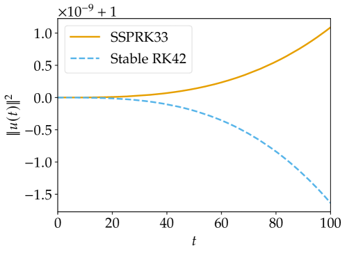
Figure 1: Discrete energies of the numerical solution of (22) using a skew-symmetric finite difference operato with $\Delta t=10^{-5}$.

4 Time-Independent Nonlinear Operators

In this section, the special case of time-independent but possibly nonlinear operators is studied. Hence,

$$\dfrac{\operatorname{d\!}{}}{\operatorname{d\!}{t}}u(t) =f(u(t)), t\in[0,T],$$ (24)

$$u(0) =u_{0},$$

is considered as special case of (1). The following result was obtained in [28, Theorem 7.1].

Theorem 4.1.

There exist first order accurate explicit Runge-Kutta methods with two stages that are strong stability preserving and energy stable for the ODE (24) with semibounded and Lipschitz continuous $f$ with $\mathinner{\!\left\lvert f\right\rvert}_{\mathrm{Lip}}\leq L$ under a time step constraint $0<\Delta t\leq\Delta t_{\mathrm{max}}\propto L^{-1}$.

The technique used in the stability proof of Theorem 4.1 can be described as follows.

1. Expand $\mathinner{\!\left\lVert u_{+}\right\rVert}^{2}-\mathinner{\!\left\lVert u_{0}\right\rVert}^{2}$ as in (7).

2. Use the Lipschitz continuity of the right-hand side of (24) in order to expand the $\Delta t^{2}$ term in a power series in $\Delta t$.

3. Use the coefficients of the scheme and signs of the dominant terms in the power series to determine conditions for energy stability.

The second step can be generalised to higher order schemes by considering analytic right-hand sides $f$ and the expansion [4, equation (313b)]

$$f(u_{i})=\sum_{\mathinner{\!\left\lvert t\right\rvert}\leq n}\Delta t^{\mathinner{\!\left\lvert t\right\rvert}-1}\frac{1}{\sigma(t)}(\Phi_{i}D)(t)\,F(t)(u_{0})+\mathcal{O}(\Delta t^{n+1}).$$ (25)

This is a sum over all trees $t$ of order $\mathinner{\!\left\lvert t\right\rvert}\leq n$, $\sigma(t)$ is the symmetry of $t$, $(\Phi_{i}D)(t)$ is the $i$-th derivative weight of $t$, and $F(t)(u_{0})$ the elementary differential associated with the tree $t$ and the right hand side $f$, evaluated at $u_{0}$.

Inserting (25) into (7) yields

$$\mathinner{\!\left\lVert u_{+}\right\rVert}^{2}-\mathinner{\!\left\lVert u_{0}\right\rVert}^{2}=2\Delta t\sum_{i=1}^{s}b_{i}\left\langle{u_{i},\,f(u_{i})}\right\rangle\\ +\sum_{\mathclap{\mathinner{\!\left\lvert t_{1}\right\rvert},\,\mathinner{\!\left\lvert t_{2}\right\rvert}\leq n}}\Delta t^{\mathinner{\!\left\lvert t_{1}\right\rvert}+\mathinner{\!\left\lvert t_{2}\right\rvert}}\sum_{i,j=1}^{s}(b_{i}b_{j}-b_{i}\,a_{ij}-b_{j}a_{ji})\frac{(\Phi_{i}D)(t_{1})\,(\Phi_{j}D)(t_{2})}{\sigma(t_{1})\sigma(t_{2})}\left\langle{F(t_{1})(u_{0}),\,F(t_{2})(u_{0})}\right\rangle\\ +\mathcal{O}(\Delta t^{n+3}).$$ (26)

Example 4.2.

For the three stage, third order method SSPRK(3,3) of [41] given by the Butcher coefficients (23), the first terms of the sum over trees in (26) are

$$\Delta t^{4}\left[\frac{1}{6}\left\langle{F(\Forest{rootedtree[]})(u_{0}),\,F(\Forest{rootedtree[[*]]})(u_{0})}\right\rangle-\frac{1}{12}\left\langle{F(\Forest{rootedtree[]})(u_{0}),\,F(\Forest{rootedtree[*,*]})(u_{0})}\right\rangle+\frac{1}{12}\mathinner{\!\left\lVert F(\Forest{rootedtree[*]})(u_{0})\right\rVert}^{2}\right]+\mathcal{O}(\Delta t^{5})\\ =\Delta t^{4}\left[\frac{1}{6}\left\langle{f,\,f^{\prime}f^{\prime}f}\right\rangle-\frac{1}{12}\left\langle{f,\,f^{\prime\prime}(f,f)}\right\rangle+\frac{1}{12}\mathinner{\!\left\lVert f^{\prime}f\right\rVert}^{2}\right]+\mathcal{O}(\Delta t^{5}).$$ (27)

The calculations leading to this expression are available in a Jupyter notebook online [31]. As an example, the coefficient $\nicefrac{{1}}{{6}}$ of the first term multiplied by $\Delta t^{4}$ can be obtained inserting the definition of the derivative weights [4, Definition 312A] and the symmetry [4, Table 301(I)] as

$$2\sum_{i,j=1}^{s}(b_{i}b_{j}-b_{i}\,a_{ij}-b_{j}a_{ji})\frac{(\Phi_{i}D)(\Forest{rootedtree[]})\,(\Phi_{j}D)(\Forest{rootedtree[[*]]})}{\sigma(\Forest{rootedtree[]})\sigma(\Forest{rootedtree[[*]]})}$$ (28)

$$= 2\sum_{i,j=1}^{s}(b_{i}b_{j}-b_{i}\,a_{ij}-b_{j}a_{ji})\frac{1\cdot\sum_{k,l=1}^{s}a_{jk}a_{kl}}{1\cdot 1}$$

Here, the factor $2$ arises because of the symmetry with respect to the order of the trees $\Forest{rootedtree[]}$ and $\Forest{rootedtree[[*]]}$. Inserting $\sum_{k,l=1}^{s}a_{jk}a_{kl}=\nicefrac{{\delta_{j3}}}{{4}}$, where $\delta_{j3}$ is the Kronecker delta, and evaluating the remaining sum yields

$$\frac{1}{2}\sum_{i}^{s}(b_{i}b_{3}-b_{i}\,a_{i3}-b_{3}a_{3i})=\frac{1}{2}\left(\frac{2}{3}-0-\frac{2}{3}\cdot\frac{1}{2}\right)=\frac{1}{6}.$$ (29)

By a suitable choice of a non-dissipative right hand side $f$ such that $\forall u\colon\left\langle{u,\,f(u)}\right\rangle=0$, the leading order term in (27) can be made positive. Hence, the energy increases for every sufficiently small time step $\Delta t$.

Of course, there are also problems for which SSPRK(3,3) is conditionally energy stable. For example, the right hand side $f\colon\mathbb{R}^{2}\to\mathbb{R}^{2}$, $f(u)=\mathinner{\!\left\lVert u\right\rVert}^{2}(-u_{2},u_{1})^{T}$, yields $-\frac{7}{12}\mathinner{\!\left\lVert u\right\rVert}^{10}+\mathcal{O}(\Delta t^{5})$ as first terms of the expansion (26).

Example 4.3.

It is appealing to choose a Runge-Kutta method such that the coefficients in front of scalar products of elementary differentials whose sign cannot be controlled vanish and such that the coefficients multiplying non-negative terms such as $\mathinner{\!\left\lVert f^{\prime}f\right\rVert}^{2}$ are negative. However, it seems difficult to do this in a way that guarantees energy stability for all semibounded $f$. For example,

$$\begin{array}[]{c|ccc}0&&&\\ \nicefrac{{3}}{{8}}&\nicefrac{{3}}{{8}}&&\\ 1&-1&2&\\ \hline\cr&\nicefrac{{1}}{{22}}&\nicefrac{{8}}{{11}}&\nicefrac{{5}}{{22}}\\ \end{array}$$ (30)

represents a three stage, second order scheme. The corresponding first terms of the sum over trees in (26) are

$$\Delta t^{4}\biggl{[}-\frac{1}{11}\mathinner{\!\left\lVert f^{\prime}f\right\rVert}^{2}\biggr{]}+\Delta t^{5}\biggl{[}-\frac{15}{176}\left\langle{f^{\prime}f,\,f^{\prime}f^{\prime}f}\right\rangle-\frac{49}{704}\left\langle{f^{\prime}f,\,f^{\prime\prime}(f,f)}\right\rangle\biggr{]}$$ (31)

$$+\Delta t^{6}\biggl{[}-\frac{45}{2816}\left\langle{f^{\prime}f,\,f^{\prime}f^{\prime\prime}(f,f)}\right\rangle-\frac{15}{176}\left\langle{f^{\prime}f,\,f^{\prime\prime}(f,f^{\prime}f)}\right\rangle-\frac{347}{16896}\left\langle{f^{\prime}f,\,f^{\prime\prime\prime}(f,f,f)}\right\rangle$$

$$\quad\quad\quad+\frac{225}{7744}\mathinner{\!\left\lVert f^{\prime}f^{\prime}f\right\rVert}^{2}+\frac{255}{30976}\left\langle{f^{\prime}f^{\prime}f,\,f^{\prime\prime}(f,f)}\right\rangle-\frac{149}{30976}\mathinner{\!\left\lVert f^{\prime\prime}(f,f)\right\rVert}^{2}\biggr{]}$$

$$+\Delta t^{7}\biggl{[}-\frac{45}{22528}\left\langle{f^{\prime}f,\,f^{\prime\prime}(f^{\prime}f^{\prime}f,f)}\right\rangle-\frac{45}{2816}\left\langle{f^{\prime}f,\,f^{\prime\prime}(f^{\prime\prime}(f,f),f)}\right\rangle$$

$$\quad\quad\quad-\frac{45}{1408}\left\langle{f^{\prime}f,\,f^{\prime\prime}(f^{\prime}f,f^{\prime}f)}\right\rangle-\frac{15}{352}\left\langle{f^{\prime}f,\,f^{\prime\prime\prime}(f^{\prime}f,f,f)}\right\rangle$$

$$\quad\quad\quad-\frac{2641}{540672}\left\langle{f^{\prime}f,\,f^{\prime\prime\prime\prime}(f,f,f,f)}\right\rangle+\frac{675}{61952}\left\langle{f^{\prime}f^{\prime}f,\,f^{\prime}f^{\prime\prime}(f,f)}\right\rangle$$

$$\quad\quad\quad+\frac{225}{3872}\left\langle{f^{\prime}f^{\prime}f,\,f^{\prime\prime}(f^{\prime}f,f)}\right\rangle+\frac{205}{22528}\left\langle{f^{\prime}f^{\prime}f,\,f^{\prime\prime\prime}(f,f,f)}\right\rangle$$

$$\quad\quad\quad+\frac{765}{495616}\left\langle{f^{\prime\prime}(f,f),\,f^{\prime}f^{\prime\prime}(f,f)}\right\rangle+\frac{255}{30976}\left\langle{f^{\prime\prime}(f,f),\,f^{\prime\prime}(f^{\prime}f,f)}\right\rangle$$

$$\quad\quad\quad-\frac{1}{16896}\left\langle{f^{\prime\prime}(f,f),\,f^{\prime\prime\prime}(f,f,f)}\right\rangle\biggr{]}$$

$$+\Delta t^{8}\biggl{[}-\frac{135}{720896}\left\langle{f^{\prime}f,\,f^{\prime}f^{\prime\prime\prime\prime}(f,f,f,f)}\right\rangle-\frac{45}{22528}\left\langle{f^{\prime}f,\,f^{\prime\prime}(f^{\prime\prime\prime}(f,f,f),f)}\right\rangle$$

$$\quad\quad\quad-\frac{135}{11264}\left\langle{f^{\prime}f,\,f^{\prime\prime}(f^{\prime\prime}(f,f),f^{\prime}f)}\right\rangle-\frac{45}{5632}\left\langle{f^{\prime}f,\,f^{\prime\prime\prime}(f^{\prime\prime}(f,f),f,f)}\right\rangle$$

$$\quad\quad\quad-\frac{45}{1408}\left\langle{f^{\prime}f,\,f^{\prime\prime\prime}(f^{\prime}f,f^{\prime}f,f)}\right\rangle-\frac{5}{352}\left\langle{f^{\prime}f,\,f^{\prime\prime\prime\prime}(f^{\prime}f,f,f,f)}\right\rangle$$

$$\quad\quad\quad-\frac{-20723}{21626880}\left\langle{f^{\prime}f,\,f^{\prime\prime\prime\prime\prime}(f,f,f,f,f)}\right\rangle+\frac{675}{495616}\left\langle{f^{\prime}f^{\prime}f,\,f^{\prime}f^{\prime\prime\prime}(f,f,f)}\right\rangle$$

$$\quad\quad\quad+\frac{675}{61952}\left\langle{f^{\prime}f^{\prime}f,\,f^{\prime\prime}(f^{\prime\prime}(f,f),f)}\right\rangle+\frac{675}{30976}\left\langle{f^{\prime}f^{\prime}f,\,f^{\prime\prime}(f^{\prime}f,f^{\prime}f)}\right\rangle$$

$$\quad\quad\quad+\frac{255}{7744}\left\langle{f^{\prime}f^{\prime}f,\,f^{\prime\prime\prime}(f^{\prime}f,f,f)}\right\rangle+\frac{22765}{7929856}\left\langle{f^{\prime}f^{\prime}f,\,f^{\prime\prime\prime\prime}(f,f,f,f)}\right\rangle$$

$$\quad\quad\quad+\frac{765}{3964928}\left\langle{f^{\prime\prime}(f,f),\,f^{\prime}f^{\prime\prime\prime}(f,f,f)}\right\rangle+\frac{765}{495616}\left\langle{f^{\prime\prime}(f,f),\,f^{\prime\prime}(f^{\prime\prime}(f,f),f)}\right\rangle$$

$$\quad\quad\quad+\frac{765}{247808}\left\langle{f^{\prime\prime}(f,f),\,f^{\prime\prime}(f^{\prime}f,f^{\prime}f)}\right\rangle+\frac{265}{61952}\left\langle{f^{\prime\prime}(f,f),\,f^{\prime\prime\prime}(f^{\prime}f,f,f)}\right\rangle$$

$$\quad\quad\quad+\frac{1667}{5947392}\left\langle{f^{\prime\prime}(f,f),\,f^{\prime\prime\prime\prime}(f,f,f,f)}\right\rangle+\frac{2025}{1982464}\mathinner{\!\left\lVert f^{\prime}f^{\prime\prime}(f,f)\right\rVert}^{2}$$

$$\quad\quad\quad+\frac{675}{61952}\left\langle{f^{\prime}f^{\prime\prime}(f,f),\,f^{\prime\prime}(f^{\prime}f,f)}\right\rangle+\frac{615}{360448}\left\langle{f^{\prime}f^{\prime\prime}(f,f),\,f^{\prime\prime\prime}(f,f,f)}\right\rangle$$

$$\quad\quad\quad+\frac{225}{7744}\mathinner{\!\left\lVert f^{\prime\prime}(f^{\prime}f,f)\right\rVert}^{2}+\frac{205}{22528}\left\langle{f^{\prime\prime}(f^{\prime}f,f),\,f^{\prime\prime\prime}(f,f,f)}\right\rangle$$

$$\quad\quad\quad+\frac{1019}{1622016}\mathinner{\!\left\lVert f^{\prime\prime\prime}(f,f,f)\right\rVert}^{2}\biggr{]}+\mathcal{O}(\Delta t^{9}).$$

Again, the calculations leading to this expression are available in a Jupyter notebook online [31]. If $\mathinner{\!\left\lVert f^{\prime}f\right\rVert}\neq 0$, the scheme is dissipative for sufficiently small time step $\Delta t>0$. Similarly, if $\mathinner{\!\left\lVert f^{\prime}f\right\rVert}=0$ and $\mathinner{\!\left\lVert f^{\prime\prime}(f,f)\right\rVert}\neq 0$, the norm of the numerical solutions cannot increase for sufficiently small $\Delta t>0$. If $f^{\prime}f=0$ and $f^{\prime\prime}(f,f)=0$, the $\Delta t^{7}$ terms vanish additionally. However, the energy of the numerical solutions increases for arbitrarily small $\Delta t>0$ if $f^{\prime}f=0$, $f^{\prime\prime}(f,f)=0$ and $\mathinner{\!\left\lVert f^{\prime\prime\prime}(f,f,f)\right\rVert}\neq 0$, since there is a positive term $\Delta t^{8}\frac{1019}{1622016}\mathinner{\!\left\lVert f^{\prime\prime\prime}(f,f,f)\right\rVert}^{2}+\mathcal{O}(\Delta t^{9})$ and all other terms vanish.

4.1 Necessary Conditions for Energy Stability

The Examples 4.2 and 4.3 demonstrate the importance of the bushy trees $\Forest{rootedtree[*]}$, $\Forest{rootedtree[*,*]}$, $\Forest{rootedtree[*,*,*]}$, $\dots$ with corresponding derivative weights $c_{i}$, $c_{i}^{2}$, $c_{i}^{3}$, $\dots$ and elementary differentials $f^{\prime}f$, $f^{\prime\prime}(f,f)$, $f^{\prime\prime\prime}(f,f,f)$ etc. While it is known that the elementary differentials are linearly independent for general right hand sides $f$ [4, Section 314], it is of interest to study the independence of these terms for semibounded $f$ and in particular for non-dissipative $f$.

In order to do that, the setting will be changed. Instead of considering a Hilbert space, $\mathcal{H}$ is a real semi inner product space. The semi inner product is still written as $\left\langle{\cdot,\,\cdot}\right\rangle$ and $\mathinner{\!\left\lVert\cdot\right\rVert}$ denotes the induced seminorm (i.e. nearly a norm but not necessarily definite). The same definitions of energy stability etc. as for inner product spaces are used. Semi inner products will be considered only in this subsection.

Theorem 4.4.

For each $k\in\mathbb{N}$, there is an autonomous ODE with semibounded right hand side $f$ in a semi inner product space such that the elementary differentials evaluated at $u_{0}$ satisfy $f^{(k)}(f,\dots,f)\neq 0$ and $f^{(l)}(f,\dots,f)=0$ for all $l\neq k$. Additionally, $\left\langle{f,\,f^{(k)}}\right\rangle=0$ and $\forall u\colon\left\langle{u,\,f(u)}\right\rangle=0$.

Proof.

Consider the space $\mathbb{R}^{3}$ equipped with the semi inner product induced by the matrix $P=\operatorname{diag}(0,1,1)$, i.e. $\left\langle{u,\,v}\right\rangle_{P}=u^{T}Pv$. Consider the ODE

$$u^{\prime}(t)=f(u(t)),\quad u(0)=\begin{pmatrix}0\\ 1\\ 0\end{pmatrix},\quad f(u)\mathrel{\mathop{\ordinarycolon}}=\begin{pmatrix}1\\ 0\\ 0\end{pmatrix}+u_{1}^{k}\begin{pmatrix}0\\ -u_{3}\\ u_{2}\end{pmatrix}.$$ (32)

The right hand side $f$ satisfies $\forall u\in\mathbb{R}^{3}\colon\left\langle{u,\,f(u)}\right\rangle_{P}=0$ and $f(u_{0})=(1,0,0)^{T}\neq 0$. Hence, for $l\in\mathbb{N}$, the $i$-th component of the elementary differential $f^{(l)}(f,\dots,f)$ evaluated at $u_{0}$ is [4, Definition 310A]

$$\left[f^{(l)}(f,\dots,f)\right]^{i}=f^{i}_{j_{1},\dots,j_{l}}f^{j_{1}}\dots f^{j_{l}}=f^{i}_{1,\dots,1}\implies f^{(l)}(f,\dots,f)=\delta_{k,l}k!\begin{pmatrix}0\\ 0\\ 1\end{pmatrix}.$$ (33)

Here, summation over repeated indices is implied, upper indices denote components, lower indices denote derivatives, and $\delta_{k,l}$ is the Kronecker delta. ∎

Remark 4.5.

If semi inner products are allowed, problems depending explicitly on time have to be considered again. Indeed, the test problem constructed in the proof of Theorem 4.4 is of this form since $u_{1}$ can be interpreted as time $t$ and the numerical approximation of $u_{1}$ is equal to $t$ if the classical condition $c_{i}=\sum_{j=1}^{s}a_{ij}$ is satisfied.

Hence, the results of section 3 can be applied, showing that there is nothing to gain if there is a $c_{i}$ distinct from the others with $b_{i}\neq 0$. Thus, it is interesting whether the independence of the elementary differentials for energy conservative right hand sides holds also in inner product spaces. Since this problem seems to be intractable with the current methods, it is left for future investigations.

Theorem 4.4 shows that the choice of elementary differentials made in Example 4.3 is possible. Hence, the method mentioned there is not energy stable for general autonomous and semibounded problems. The basic argument used there can be formulated as follows.

Theorem 4.6.

Consider a Runge-Kutta method with order of accuracy at least two. If there is a $k\in\mathbb{N}$ such that the Butcher coefficients satisfy

$$\sum_{i,j=1}^{s}(b_{i}b_{j}-b_{i}\,a_{ij}-b_{j}\,a_{ji})c_{i}^{k}c_{j}^{k}>0,$$ (34)

then the method is not energy stable for general autonomous and semibounded ODEs in semi inner product spaces.

Proof.

Since the method is at least second order accurate, the lowest order term in the sum involving trees in (26) vanishes since

$$\sum_{i,j=1}^{s}(b_{i}b_{j}-b_{i}\,a_{ij}-b_{j}a_{ji})(\Phi_{i}D)(\Forest{rootedtree[]})\,(\Phi_{j}D)(\Forest{rootedtree[]}) =\sum_{i,j=1}^{s}(b_{i}b_{j}-b_{i}\,a_{ij}-b_{j}a_{ji})$$ (35)

$$=\left(\sum_{i=1}^{s}b_{i}\right)^{2}-2\sum_{i=1}^{s}b_{i}c_{i}=1-2\cdot\frac{1}{2}=0.$$

Because of Theorem 4.4, it is possible to choose $f$ such that the remaining terms all vanish except the one corresponding to the bushy tree with $k$ leaves. While this is not formulated directly there, a close inspection of the proof reveals that this is indeed true. For example, one can choose $f$ so that $f^{\prime}=0$ and $\left\langle{f,\,f^{\prime}f^{\prime\prime}(f,f)}\right\rangle=0$ while $f\neq 0$ and $f^{\prime\prime}(f,f)\neq 0$.

By choosing such an $f$ all terms of order up to $\Delta t^{2k+1}$ vanish and (26) takes the form

$$\mathinner{\!\left\lVert u_{+}\right\rVert}^{2}-\mathinner{\!\left\lVert u_{0}\right\rVert}^{2}=\Delta t^{2k+2}\underbrace{\sum_{i,j=1}^{s}(b_{i}b_{j}-b_{i}\,a_{ij}-b_{j}a_{ji})c_{i}^{k}c_{j}^{k}\mathinner{\!\left\lVert f^{(k)}(f,\dots,f)\right\rVert}^{2}}_{>0}+\mathcal{O}(\Delta t^{2k+3}).$$ (36)

Hence, $\mathinner{\!\left\lVert u_{+}\right\rVert}^{2}>\mathinner{\!\left\lVert u_{0}\right\rVert}^{2}$ for arbitrarily small $\Delta t>0$. ∎

Theorem 4.6 implies in particular that $\sum_{i,j=1}^{s}(b_{i}b_{j}-b_{i}\,a_{ij}-b_{j}a_{ji})c_{i}^{k}c_{j}^{k}$ must be non-positive for B-stable methods. This is related to algebraically stable schemes, where the matrix with entries $(b_{i}b_{j}-b_{i}\,a_{ij}-b_{j}a_{ji})$ is negative semidefinite. It can be proved that B-stable schemes are indeed algebraically stable if certain additional (technical) assumptions are satisfied, e.g. if the method is non-confluent [16, Corollary IV.12.14] or irreducible [16, Theorem IV.12.18].

Example 4.7.

For the B-stable but not algebraically stable reducible schemes with $A=\begin{pmatrix}1/2&0\\ 0&1/2\end{pmatrix}$, $b=(2,-1)^{T}$ [7, page 80] and $A=\begin{pmatrix}1/2&0\\ 1/4&1/4\end{pmatrix}$, $b=(1/2,1/2)^{T}$ [16, Table IV.12.2], the terms $\sum_{i,j=1}^{s}(b_{i}b_{j}-b_{i}\,a_{ij}-b_{j}a_{ji})(\Phi_{i}D)(t_{1})\,(\Phi_{j}D)(t_{2})$ vanish, exactly as for the implicit midpoint method to which these schemes can be reduced.

While explicit Runge-Kutta methods cannot be algebraically stable, which would imply unconditional energy stability for all semibounded problems, it is interesting to study whether they can be stable for these problems under a suitable time step restriction. Theorem 4.1 proves that there are indeed conditionally energy stable schemes of first order. For higher order schemes, it remains to check the condition given in Theorem 4.6. While this can be done for every scheme given explicitly, there are some results for general classes of schemes.

Theorem 4.8.

Consider an explicit Runge-Kutta method. Assume that there is a unique ${i_{\mathrm{max}}}$ such that $\mathinner{\!\left\lvert c_{i_{\mathrm{max}}}\right\rvert}=\max_{i}\mathinner{\!\left\lvert c_{i}\right\rvert}$ and that $b_{i_{\mathrm{max}}}\neq 0$. Then there is a $k\in\mathbb{N}$ such that (34) is satisfied. Hence, if the method is at least second order accurate, it is not energy stable for general autonomous and semibounded ODEs in semi inner product spaces.

Proof.

The expression on the left hand side of (34) can be written as

$$\bigl{(}b^{T}c^{k}\bigr{)}^{2}-2\bigl{(}c^{k}\bigr{)}^{T}\operatorname{diag}(b)Ac^{k},$$ (37)

where the exponentiation is performed componentwise. Using the given assumptions,

$$\left(\frac{c}{c_{i_{\mathrm{max}}}}\right)^{k}\to e_{i_{\mathrm{max}}},\quad k\to\infty,$$ (38)

where $e_{i_{\mathrm{max}}}$ is the standard unit vector with components $(e_{i_{\mathrm{max}}})_{j}=\delta_{j,{i_{\mathrm{max}}}}$. Since the Runge-Kutta scheme is explicit, $A$ is a strictly lower triangular matrix and $e_{i_{\mathrm{max}}}^{T}\operatorname{diag}(b)Ae_{i_{\mathrm{max}}}=0$. Because of $b^{T}e_{i_{\mathrm{max}}}=b_{i_{\mathrm{max}}}\neq 0$,

$$\biggl{(}\frac{b^{T}c^{k}}{c_{i_{\mathrm{max}}}}\biggr{)}^{2}-2\frac{(c^{k})^{T}}{c_{i_{\mathrm{max}}}^{k}}\operatorname{diag}(b)A\frac{c^{k}}{c_{i_{\mathrm{max}}}^{k}}\to\bigl{(}b^{T}e_{i_{\mathrm{max}}}\bigr{)}^{2}-2e_{i_{\mathrm{max}}}^{T}\operatorname{diag}(b)Ae_{i_{\mathrm{max}}}^{k}=b_{i_{\mathrm{max}}}^{2}\neq 0,$$ (39)

for $k\to\infty$. Hence, there is a $k\in\mathbb{N}$ such that (34) is satisfied. ∎

Remark 4.9.

Theorem 4.8 can also be applied to many confluent methods such as the ten-stage, fourth order, explicit strong stability preserving method SSPRK(10,4) of [18]. Indeed, ${i_{\mathrm{max}}}=10$, $c_{i_{\mathrm{max}}}=1$, and $b_{i_{\mathrm{max}}}=\frac{1}{10}$ in that case. That this scheme is not energy stable for autonomous and semibounded problems has also been proved using some specific counterexamples in [28, Sections 4.3 and 6].

Remark 4.10.

The argument used to prove Theorem 4.8 can also be applied to implicit Runge-Kutta methods with $a_{{i_{\mathrm{max}}},{i_{\mathrm{max}}}}=0$.

4.2 Sufficient Conditions for Energy Stability

Theorem 4.8 does not imply that all explicit Runge-Kutta methods of order two or greater cannot be energy stable.

Example 4.11.

The Runge-Kutta method with Butcher coefficients

$$\begin{array}[]{c|cccc}0&&&&\\ 1&1&&&\\ 0&1&-1&&\\ 1&-1&1&1&\\ \hline\cr&\nicefrac{{1}}{{4}}&\nicefrac{{1}}{{4}}&\nicefrac{{1}}{{4}}&\nicefrac{{1}}{{4}}\\ \end{array}$$ (40)

has four stages and is second order accurate. Since $c_{2}=1=c_{4}$, it does not satisfy the assumptions of Theorem 4.8. Because $c_{i}\in\left\{0,1\right\}$, we have $c^{k}=c$ for $k\in\mathbb{N}$. Hence, it suffices to consider $k=1$ in (34), i.e.

$$\sum_{i,j=1}^{s}(b_{i}b_{j}-b_{i}\,a_{ij}-b_{j}\,a_{ji})c_{i}c_{j}=-\frac{1}{4}<0.$$ (41)

Thus, the sum in (34) is negative for all $k\in\mathbb{N}$.

Theorem 4.12.

The Runge-Kutta method given in Example 4.11 is conditionally energy stable with respect to autonomous ODEs (24) with analytical and semibounded right hand side.

Proof.

Since the right hand side $f$ is analytical, the energy difference after one time step can be expanded as in (26). Because of the semiboundedness of $f$, the term proportional to $\Delta t$ is non-positive.

There are no inner products between $f=F(\Forest{rootedtree[]})$ and higher order elementary differentials in the remaining terms because

$$\sum_{i,j=1}^{s}(b_{i}b_{j}-b_{i}a_{ij}-b_{j}a_{ji})\frac{(\Phi_{i}D)(\Forest{rootedtree[]})\,(\Phi_{j}D)(t_{2})}{\sigma(\Forest{rootedtree[]})\,\sigma(t_{2})}=\sum_{j=1}^{s}\underbrace{\biggl{(}b_{j}-\sum_{i=1}^{s}b_{i}a_{ij}-b_{j}c_{j}\biggr{)}}_{=0}\frac{(\Phi_{j}D)(t_{2})}{\sigma(t_{2})},$$ (42)

which can be computed explicitly. The first remaining terms are of the form

$$-\frac{1}{4}\Delta t^{4}\mathinner{\!\left\lVert f^{\prime}f\right\rVert}^{2}+\Delta t^{5}\biggl{[}-\frac{1}{2}\left\langle{f^{\prime}f,\,f^{\prime}f^{\prime}f}\right\rangle-\frac{1}{4}\left\langle{f^{\prime}f,\,f^{\prime\prime}(f,f)}\right\rangle\biggr{]}$$ (43)

$$+\Delta t^{6}\biggl{[}\frac{1}{4}\left\langle{f^{\prime}f,\,f^{\prime}f^{\prime}f^{\prime}f}\right\rangle-\frac{1}{4}\left\langle{f^{\prime}f,\,f^{\prime}f^{\prime\prime}(f,f)}\right\rangle-\frac{1}{4}\left\langle{f^{\prime}f,\,f^{\prime\prime}(f^{\prime}f,f)}\right\rangle$$

$$\qquad\quad-\frac{1}{12}\left\langle{f^{\prime}f,\,f^{\prime\prime\prime}(f,f,f)}\right\rangle+\frac{1}{2}\mathinner{\!\left\lVert f^{\prime}f^{\prime}f\right\rVert}^{2}-\frac{1}{4}\left\langle{f^{\prime}f^{\prime}f,\,f^{\prime\prime}(f,f)}\right\rangle-\frac{1}{16}\mathinner{\!\left\lVert f^{\prime\prime}(f,f)\right\rVert}^{2}\biggr{]}.$$

If $f^{\prime}f\neq 0$, the $\Delta t^{4}$ term dominates the other ones for sufficiently small $\Delta t>0$ and the scheme is energy stable. If $f^{\prime}f=0$ and $f^{\prime\prime}(f,f)\neq 0$, the $\Delta t^{4}$, $\Delta t^{5}$, and most of the $\Delta t^{6}$ terms vanish. Only $-\frac{1}{16}\Delta t^{6}\mathinner{\!\left\lVert f^{\prime\prime}(f,f)\right\rVert}<0$ remains and dominates higher order terms, resulting in a stable scheme for small $\Delta t>0$.

This argument can be applied similarly to all other terms. Suppose that $f^{\prime}f=\dots=f^{(k-1)}(f,\dots,f)=0$ and $f^{(k)}(f,\dots,f)\neq 0$. The terms up to (and including) $\mathcal{O}(\Delta t^{2k+1})$ vanish, since (as described at the beginning of the proof) for this method, the series (26) does not include any terms involving an inner product of $f$ and other elementary differentials. Most of the $\Delta t^{2k+2}$ terms vanish too, except the one proportional to $\mathinner{\!\left\lVert f^{(k)}(f,\dots,f)\right\rVert}$. Because $\sum_{i,j=1}^{s}(b_{i}b_{j}-b_{i}a_{ij}-b_{j}a_{ji})c_{i}^{k}c_{j}^{k}<0$, this term is negative and dominates higher order terms. Hence, the scheme is energy stable for sufficiently small $\Delta t>0$. ∎

The key ingredients of the proof of Theorem 4.12 are distilled in

Proposition 4.13.

Consider a second or third order accurate explicit Runge-Kutta method satisfying

$$\bullet\forall i\in\left\{1,\dots,s\right\}\colon b_{i}\geq 0, \bullet\forall j\in\left\{1,\dots,s\right\}\colon b_{j}-\sum_{i=1}^{s}b_{i}a_{ij}-b_{j}c_{j}=0,$$

$$\bullet\forall i\in\left\{1,\dots,s\right\}\colon c_{i}=\sum_{j=1}^{s}a_{ij}, \bullet\forall k\in\mathbb{N}\colon\text{The sum in \eqref{eq:sign-condition} is negative}.$$

Such a scheme is conditionally energy stable for any autonomous ODE (24) with right hand side that is analytical and semibounded with respect to an inner product.

The proof is basically the same as that of Theorem 4.12. The restriction to second and third order accurate schemes is explained in Section 4.3 below.

Remark 4.14.

Since infinitely many constraints have to be satisfied to apply Proposition 4.13, it is useful to consider additional simplifying assumptions/constraints in order to find feasible solutions. The Runge-Kutta method given in Example 4.11 and other schemes have been constructed using the following additional steps.

• Because of Theorem 4.8, the node with biggest absolute value should appear at least twice. In order to facilitate the search for a solution, it has been useful to choose the nodes $c_{i}$ manually. Here, the biggest node is chosen as $1$ (twice). In numerical experiments, it seemed to be useful/necessary to specify also the node $0$ twice.

• The sum in (34) with $k=1$ has to be negative. Additionally, the same sum involving only the nodes $0$ and $1$ should be negative. In numerical experiments, this additional condition has often be sufficient to guarantee that the sum in (34) is negative for general $k\in\mathbb{N}$.

Example 4.15.

The third order accurate Runge-Kutta method with Butcher coefficients

$$\begin{array}[]{c|ccccc}0&&&&&\\ \nicefrac{{1}}{{2}}&\nicefrac{{1}}{{2}}&&&\\ 1&1&&&\\ 0&1&0&-1&\\ 1&-3&2&1&1\\ \hline\cr&0&\nicefrac{{2}}{{3}}&0&\nicefrac{{1}}{{6}}&\nicefrac{{1}}{{6}}\\ \end{array}$$ (44)

has been constructed using the approach just described. It is energy stable for autonomous ODEs (24) with analytical and semibounded right hand side in inner product spaces if the time step $\Delta t>0$ is sufficiently small. Indeed, since

$$\sum_{i,j=1}^{s}(b_{i}b_{j}-b_{i}\,a_{ij}-b_{j}\,a_{ji})c_{i}^{k}c_{j}^{k}=-\frac{11}{36}-\frac{4}{9}2^{-k}\bigl{(}1-2^{-k}\bigr{)}<0,$$ (45)

the sum in (34) is negative for general $k\in\mathbb{N}$ and Proposition 4.13 can be applied.

4.3 Limitations for Higher Order Schemes

The conditions listed in Proposition 4.13 are not sufficient to create energy stable fourth order methods, since the coefficient of $\mathinner{\!\left\lVert f^{\prime}f\right\rVert}^{2}$ in the expansion (26) vanishes because of accuracy constraints. However, terms like $\left\langle{f^{\prime}f,\,f^{\prime}f^{\prime}f}\right\rangle$ etc. appear later, which cannot be controlled in general. Hence, one has to impose additionally that all scalar products of $f^{\prime}f$ with higher order differentials vanish. Because of

$$\sum_{i,j=1}^{s}(b_{i}b_{j}-b_{i}a_{ij}-b_{j}a_{ji})\frac{(\Phi_{i}D)(\Forest{rootedtree[*]})\,(\Phi_{j}D)(t_{2})}{\sigma(\Forest{rootedtree[*]})\,\sigma(t_{2})}\\ =\sum_{j=1}^{s}\biggl{(}b_{j}\sum_{i=1}^{s}c_{i}-\sum_{i=1}^{s}b_{i}c_{i}a_{ij}-b_{j}\sum_{i=1}^{s}a_{ji}c_{i}\biggr{)}\frac{(\Phi_{j}D)(t_{2})}{\sigma(t_{2})},$$ (46)

this additional constraint is

$$b_{j}\sum_{i=1}^{s}c_{i}-\sum_{i=1}^{s}b_{i}c_{i}a_{ij}-b_{j}\sum_{i=1}^{s}a_{ji}c_{i}=0.$$ (47)

By summing over $j$ and using the order conditions for order 3, it becomes clear that some nodes $c_{i}$ must be negative if this constraint should be satisfied.

Nevertheless, even this additional constraint does not suffice to guarantee energy stability. Indeed, terms involving higher order differentials of the form $\mathinner{\!\left\lVert f^{\prime}f^{\prime}f\right\rVert}^{2}$ appear and cannot be controlled by the previous terms with negative coefficients.

5 Unconditional Stability of Explicit Runge-Kutta Discretizations

In this section we investigate the possibility of obtaining unconditional stability with explicit Runge-Kutta methods. It is usually true in numerical analysis that explicit methods can be only conditionally stable. The following (unsurprising) theorem confirms this view, in the context of the linear autonomous initial-value problem:

$$\begin{aligned} \dfrac{\operatorname{d\!}{}}{\operatorname{d\!}{t}}u(t)&=Lu(t),&&t\in[0,T],\\ u(0)&=u_{0},\end{aligned}$$ (48)

Theorem 5.1.

Let an at least first order accurate explicit Runge-Kutta method and constant (possibly complex) matrix $L\neq 0$ be given. Then, there exist initial values $u_{0}$ and a step size $\Delta t_{*}(A,b,L)$ such that the numerical solution $u^{n}$ of (48) blows up as $n\to\infty$ for any $\Delta t>\Delta t_{*}$.

Proof.

An $s$-stage explicit Runge-Kutta method applied to (48) gives the solution $u^{n+1}=R(\Delta tL)u^{n}$, where $R(z)=\sum_{j=0}^{d}\alpha_{j}z^{j}$ is a polynomial with degree $d\leq s$ and $\alpha_{0}=\alpha_{1}=1$. Two cases can occur.

1. $L$ has an eigenvalue $\lambda\neq 0$ with eigenvector $u_{0}$: Then, $R(\Delta tL)u_{0}=(I+\alpha_{1}\Delta tL+\dots+\alpha_{d}\Delta t^{d}L^{d})u_{0}=(I+\alpha_{1}\Delta t\lambda+...+\alpha_{d}\Delta t^{d}\lambda^{d})u_{0}$. Thus, $R(\Delta tL)^{n}u_{0}\to\infty$ for $n\to\infty$ if $\Delta t$ is big enough.

2. Zero is the only eigenvalue of $L$: Then, there is a vector $u_{0}$ such that $Lv\neq 0$ but $L^{2}v=0$ (consider the Jordan canonical form). Thus, $R(\Delta tL)^{n}u_{0}=(1+n\alpha_{1}\Delta tL)u_{0}\to\infty$ for $n\to\infty$ if $\Delta t$ is big enough. ∎

In practice, due to rounding errors, it is reasonable to expect a blowup for almost all initial data.

5.1 Nonlinear Problems

It is natural to ask if a result like Theorem 5.1 holds when $L$ is allowed to be nonlinear. It seems quite natural to expect that the answer is yes. However, we have the following result:

Theorem 5.2.

There exists an explicit Runge-Kutta method and non-trivial function $f(u)$ such that the numerical solution of $u^{\prime}(t)=f(u)$ remains bounded as $n\to\infty$ for every step size $\Delta t$ and for every initial value.

Proof.

We prove this result by constructing an example – the only example of which we are presently aware. We take the explicit midpoint Runge-Kutta method

$$y_{2}=u^{n}+\frac{\Delta t}{2}f(u^{n}),\qquad u^{n+1}=u^{n}+\Delta tf(y_{2}),$$ (49)

and the ODEs

$$\begin{pmatrix}u_{1}^{\prime}(t)\\ u_{2}^{\prime}(t)\end{pmatrix}=\frac{1}{u_{1}^{2}+u_{2}^{2}}\begin{pmatrix}-u_{2}\\ u_{1}\end{pmatrix}.$$ (50)

Direct calculation of the change in energy over a step (using (7)) reveals that it is constant:

$$\mathinner{\!\left\lVert u_{+}\right\rVert}^{2}-\mathinner{\!\left\lVert u_{0}\right\rVert}^{2}=\left\langle{f(u_{0}),\,f(y_{2})}\right\rangle-\left\langle{f(y_{2}),\,f(y_{2})}\right\rangle=0.$$ (51)

∎

In fact, we can write explicitly the solution obtained for the example in the proof. For the general initial value $u_{0}=r_{0}(\cos(\theta_{0}),\sin(\theta_{0}))^{T}$, the numerical solution of (50) obtained with the explicit midpoint RK method is

$$u^{n} =r_{0}\begin{pmatrix}\cos(\theta_{0}+n\theta_{h})\\ \sin(\theta_{0}+n\theta_{h})\end{pmatrix},\quad\text{where }\quad\theta_{h}=\arccos\frac{r^{2}-\frac{\Delta t^{2}}{4r^{2}}}{r^{2}+\frac{\Delta t^{2}}{4r^{2}}}.$$ (52)

This example is quite remarkable, and naturally leads one to wonder if others like it exist. If we assume the numerical energy is constant, then the problem must also be energy conservative since the Runge-Kutta scheme converges to the analytical solution (if the right hand side is locally Lipschitz continuous). In $\mathbb{R}^{2}$, every energy conservative problem is of the form

$$\begin{pmatrix}u_{1}^{\prime}(t)\\ u_{2}^{\prime}(t)\end{pmatrix}=g(u)\begin{pmatrix}-u_{2}\\ u_{1}\end{pmatrix},$$ (53)

where $g$ is a scalar valued function. We have the following uniqueness result.

Theorem 5.3.

Let a consistent two-stage explicit Runge-Kutta method and a function $g\colon\mathbb{R}^{2}\to\mathbb{R}$ be given. Consider the ODE (53) and suppose that the numerical solution satisfies $\mathinner{\!\left\lVert u^{n}\right\rVert}=\mathinner{\!\left\lVert u_{0}\right\rVert}$ for all step sizes $\Delta t$ and all $n$.

1. If $g$ is not identically zero, then the Runge-Kutta method must be the explicit midpoint method (49).

2. If $g\colon\mathbb{R}^{2}\setminus\left\{0\right\}\to\mathbb{R}$ is analytic, then $g$ must be a scalar multiple of $u\mapsto\mathinner{\!\left\lVert u\right\rVert}^{-2}$.

Proof.

a) For brevity, let $r=g(u_{0})$ and $s=g(y_{2})=g(u_{0}+a_{21}\Delta tf(u_{0}))$.

$$\left\langle{f_{1},\,f_{1}}\right\rangle =\mathinner{\!\left\lVert u_{0}\right\rVert}^{2}r^{2},$$ (54)

$$\left\langle{f_{2},\,f_{2}}\right\rangle =\mathinner{\!\left\lVert u_{0}\right\rVert}^{2}s^{2}(1+a_{21}^{2}\Delta t^{2}r^{2}),$$

$$\left\langle{f_{1},\,f_{2}}\right\rangle =\mathinner{\!\left\lVert u_{0}\right\rVert}^{2}rs.$$

Thus energy is conserved if and only if (after dividing through by $\mathinner{\!\left\lVert u_{0}\right\rVert}^{2}$)

$$2b_{2}a_{21}rs=b_{1}^{2}r^{2}+b_{2}^{2}s^{2}(1+a_{21}^{2}\Delta t^{2}r^{2})+2b_{1}b_{2}rs=0.$$ (55)

This is a quadratic equation in $s$, which has real roots only if

$$b_{2}^{2}r^{2}(b_{1}-a_{21})^{2}\geq b_{1}^{2}b_{2}^{2}r^{2}(1+a_{21}^{2}\Delta t^{2}r^{2}).$$ (56)

This cannot hold for all $\Delta t$ unless the term involving $\Delta t$ vanishes. So we must have $b_{1}b_{2}a_{21}r=0$. The case $r=0$ is ruled out by assumption, while $b_{2}=0$ implies $r=0$ by (55). Taking $a_{21}=0$ implies (by (55)) that the ratio $r/s$ is equal to a constant independent of $\Delta t$ or $u$, which is not possible. Thus we must have $b_{1}=0$; consistency then requires $b_{2}=1$. This implies that $s=0$ (trivial) or that

$$g(u+a_{21}\Delta tf(u))(1+a_{21}^{2}\Delta t^{2}(g(u))^{2})=2a_{21}g(u).$$ (57)

Considering $\Delta t\to 0$, we find that necessarily $a_{21}=1/2$; the resulting method is the midpoint Runge-Kutta method (49).

b) It suffices to consider $g\neq 0$. Expanding (57) with $a_{21}=\nicefrac{{1}}{{2}}$ as required by a) yields

$$\sum_{k\geq 0}\frac{1}{k!}2^{-k}\Delta t^{k}g^{(k)}(f,\dots,f)\bigl{(}1+2^{-2}\Delta t^{2}g^{2}\bigr{)}=g.$$ (58)

This is equivalent to

$$\frac{1}{2}\Delta tg^{\prime}f+\sum_{k\geq 2}2^{-k}\Delta t^{k}\left(\frac{1}{k!}g^{(k)}(f,\dots,f)+\frac{1}{(k-2)!}g^{2}g^{(k-2)}(f,\dots,f)\right)=0.$$ (59)

Since this has to hold for all $\Delta t$,

$$g^{\prime}f=0,\quad\forall k\geq 2\colon g^{(k)}(f,\dots,f)=-\frac{k!}{(k-2)!}g^{2}g^{(k-2)}(f,\dots,f).$$ (60)

This infinite set of conditions determines $g$ uniquely up to a scalar multiple. Indeed, using polar coordinates $(r,\theta)$ for $u$, the condition $g^{\prime}f=0$ implies that $g$ does not depend on the angle $\theta$, i.e. that $g$ is radially symmetric. Hence, $g$ can be considered as a function depending only on the radius $r$ in (57). Expanding this analytic function $(0,\infty)\to\mathbb{R}$ in (57), all derivatives at an arbitrary point are fixed. Hence, $g$ is determined up to a multiplicative factor. ∎

Remark 5.4.

Theorem 5.3 holds also for $\mathbb{R}^{3}$ instead of $\mathbb{R}^{2}$. Indeed, the action of an arbitrary skew-symmetric matrix is equivalent to the cross product with an associated vector in $\mathbb{R}^{3}$. The span of this vector is irrelevant for the considered problem.

5.2 Numerical Experiments

Here, some numerical experiments using the ODE (50) are performed. The explicit midpoint method (49), the third order strong stability preserving method SSPRK33 of [41], and the energy stable second and third order methods given in Examples 4.11 and 4.15 are applied with constant time steps $\Delta t\in\left\{10^{-1},10^{-5}\right\}$. The methods are implemented using quadruple precision numbers Float128 in the package DifferentialEquations.jl [27] in Julia [1]. The source code for these numerical experiments is available at [31].

The results displayed in Figure 2 confirm the analytical results: The energy grows monotonically for SSPRK33, stays constant for the midpoint rule and decays for the energy stable methods.

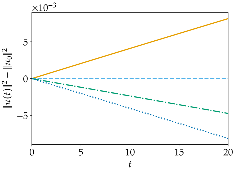
(a) $\Delta t=10^{-1}$.

(b) $\Delta t=10^{-5}$.

Figure 2: Evolution of the energy of numerical solutions for the nonlinear problem (50).

Remark 5.5.

The first terms of the expansion (26) for the test problem (50) and the second order method of Example 4.11 are

$$-\frac{1}{4}\Delta t^{4}\mathinner{\!\left\lVert f^{\prime}f\right\rVert}^{2}+\mathcal{O}(\Delta t^{5})=-\frac{1}{4}\Delta t^{4}\mathinner{\!\left\lVert u\right\rVert}^{-6}+\mathcal{O}(\Delta t^{5}).$$ (61)

Hence, it can be verified easily that the method is conditionally energy stable. Similarly, the first terms for the third order method of Example 4.15 are

$$-\frac{5}{12}\Delta t^{4}\mathinner{\!\left\lVert f^{\prime}f\right\rVert}^{2}+\mathcal{O}(\Delta t^{5})=-\frac{5}{12}\Delta t^{4}\mathinner{\!\left\lVert u\right\rVert}^{-6}+\mathcal{O}(\Delta t^{5}).$$ (62)

Thus, this method is energy stable, too. Additionally, this explains why the third order method is more (nearly twice as) dissipative than the second order one in Figure 2.

6 Summary and Conclusions

As we have seen, explicit Runge-Kutta methods that are conditionally energy stable for all nonlinear autonomous semibounded problems (with at least Lipschitz continuous right-hand sides) are rare, but they do exist. The existence of explicit energy stable methods for non-autonomous problems (even in the linear setting) is still an open question. Any explicit energy stable method for non-autonomous problems must be confluent, since otherwise it would need to be unconditionally stable (see Theorem 3.10). Nevertheless, there is at least a second order accurate scheme that is energy stable for a restricted class of relevant problems (see Proposition 3.7).

For nonlinear autonomous problems, our analysis is based on the series expansion (26) of the change in energy. Besides deriving necessary conditions, Proposition 4.13 and Remark 4.14 list sufficient conditions and approaches that can be used to create energy stable second and third order methods (see Theorem 4.12 and Example 4.15). This approach could also be used to construct methods that are energy stable for a particular problem, if one knows which elementary differentials of $f$ vanish.

Some of our results seem at first glance surprising or counter-intuitive. A common intuition is that linear problems are easier than nonlinear problems. But if explicit time dependence is allowed, the linear setting becomes much more challenging: notice that the derived necessary conditions for energy stability in this case are more restrictive than for autonomous nonlinear problems. In a similar vein, a particular nonlinear ODE may be easier to deal with than even any linear autonomous ODE, as demonstrated by Theorem 5.2 (showing unconditional stability for a specific nonlinear ODE and explicit RK method) and Theorem 5.1 (showing that no explicit RK method is unconditionally stable for any non-trivial linear problem).

In the literature, the assumption of non-confluence is often merely technical and not necessary. In contrast, in our study of energy stability for non-autonomous problems we have found that confluence is an important property, and that certain confluent Runge-Kutta methods (more specifically, methods with no distinct quadrature node) can have stability properties that are impossible for non-confluent methods.

While developing many answers, this article has also revealed several open questions and directions of further research. First of all, an obvious question concerns the possibility of fourth or higher order explicit Runge-Kutta that are conditionally energy stable (at least for autonomous problems). From a practical point of view, it would be interesting to perform a computational optimization of energy stable Runge-Kutta methods and compare them to state of the art schemes that are not energy stable.

More theoretically interesting questions concern the independence of the elementary differentials for conservative problems and the existence or uniqueness of unconditionally stable explicit Runge-Kutta methods and associated nonlinear right hand sides. For instance, if it were possible to choose the values of the elementary differentials independently while also choosing $f$ to conserve energy, then it would be possible (in principle) to construct, for each Runge-Kutta method (including all explicit methods), a problem for which that method is unconditionally energy conservative.

Appendix A Details of the Proof of Proposition 3.7

The change of the norm for general $L$ can be calculated explicitly as

$$\mathinner{\!\left\lVert u_{+}\right\rVert}^{2}-\mathinner{\!\left\lVert u_{0}\right\rVert}^{2}=\Delta t\biggl{(}\langle{u_{0},\,L_{0}u_{0}}\rangle+\langle{u_{0},\,L_{1}u_{0}}\rangle\biggr{)}$$ (16)

$$\quad+\frac{1}{2}\Delta t^{2}\biggl{(}\langle{u_{0},\,L_{0}^{2}u_{0}}\rangle-\langle{u_{0},\,L_{0}L_{1}u_{0}}\rangle+\langle{u_{0},\,L_{1}L_{0}u_{0}}\rangle+\langle{u_{0},\,L_{1}^{2}u_{0}}\rangle$$

$$\qquad\quad+\frac{1}{2}\mathinner{\!\left\lVert L_{0}u_{0}\right\rVert}^{2}+\langle{L_{0}u_{0},\,L_{1}u_{0}}\rangle+\frac{1}{2}\mathinner{\!\left\lVert L_{1}u_{0}\right\rVert}^{2}\biggr{)}$$

$$\quad+\frac{1}{2}\Delta t^{3}\biggl{(}-\langle{u_{0},\,L_{0}L_{1}L_{0}u_{0}}\rangle+\langle{u_{0},\,L_{1}L_{0}^{2}u_{0}}\rangle-\langle{u_{0},\,L_{1}L_{0}L_{1}u_{0}}\rangle+\langle{u_{0},\,L_{1}^{2}L_{0}u_{0}}\rangle$$

$$\qquad\quad+\frac{1}{2}\langle{L_{0}u_{0},\,L_{0}^{2}u_{0}}\rangle-\frac{1}{2}\langle{L_{0}u_{0},\,L_{0}L_{1}u_{0}}\rangle+\frac{1}{2}\langle{L_{0}u_{0},\,L_{1}L_{0}u_{0}}\rangle+\frac{1}{2}\langle{L_{0}u_{0},\,L_{1}^{2}u_{0}}\rangle$$

$$\qquad\quad+\frac{1}{2}\langle{L_{0}^{2}u_{0},\,L_{1}u_{0}}\rangle+\frac{1}{2}\langle{L_{1}u_{0},\,L_{1}L_{0}u_{0}}\rangle-\frac{1}{2}\langle{L_{1}u_{0},\,L_{0}L_{1}u_{0}}\rangle+\frac{1}{2}\langle{L_{1}u_{0},\,L_{1}^{2}u_{0}}\rangle\biggr{)}$$

$$\quad+\frac{1}{2}\Delta t^{4}\biggl{(}-\langle{u_{0},\,L_{1}L_{0}L_{1}L_{0}u_{0}}\rangle-\frac{1}{2}\langle{L_{0}u_{0},\,L_{0}L_{1}L_{0}u_{0}}\rangle+\frac{1}{2}\langle{L_{0}u_{0},\,L_{1}L_{0}^{2}u_{0}}\rangle$$

$$\qquad\quad-\frac{1}{2}\langle{L_{0}u_{0},\,L_{1}L_{0}L_{1}u_{0}}\rangle+\frac{1}{2}\langle{L_{0}u_{0},\,L_{1}^{2}L_{0}u_{0}}\rangle+\frac{1}{8}\mathinner{\!\left\lVert L_{0}^{2}u_{0}\right\rVert}^{2}-\frac{1}{4}\langle{L_{0}^{2}u_{0},\,L_{0}L_{1}u_{0}}\rangle$$

$$\qquad\quad+\frac{1}{4}\langle{L_{0}^{2}u_{0},\,L_{1}L_{0}u_{0}}\rangle+\frac{1}{4}\langle{L_{0}^{2}u_{0},\,L_{1}^{2}u_{0}}\rangle+\frac{1}{2}\langle{L_{1}u_{0},\,L_{1}L_{0}^{2}u_{0}}\rangle$$

$$\qquad\quad-\frac{1}{4}\langle{L_{0}L_{1}u_{0},\,L_{1}L_{0}u_{0}}\rangle+\frac{1}{8}\mathinner{\!\left\lVert L_{1}L_{0}u_{0}\right\rVert}^{2}+\frac{1}{4}\langle{L_{1}L_{0}u_{0},\,L_{1}^{2}u_{0}}\rangle$$

$$\qquad\quad-\frac{1}{2}\langle{L_{1}u_{0},\,L_{0}L_{1}L_{0}u_{0}}\rangle+\frac{1}{2}\langle{L_{1}u_{0},\,L_{1}^{2}L_{0}u_{0}}\rangle-\frac{1}{2}\langle{L_{1}u_{0},\,L_{1}L_{0}L_{1}u_{0}}\rangle$$

$$\qquad\quad+\frac{1}{8}\mathinner{\!\left\lVert L_{0}L_{1}u_{0}\right\rVert}^{2}-\frac{1}{4}\langle{L_{0}L_{1}u_{0},\,L_{1}^{2}u_{0}}\rangle+\frac{1}{8}\mathinner{\!\left\lVert L_{1}^{2}u_{0}\right\rVert}^{2}\biggr{)}+\mathcal{O}(\Delta t^{5}).$$

This calculation is also provided as Mathematica notebook in the accompagnying repository [31]. Using the skew-symmetry of the operators $L_{0},L_{1}$, the term proportional to $\Delta t$ vanishes. Since $L_{0}$ and $L_{1}$ commute, the $\Delta t^{2}$ term can be simplified to

$$+\frac{1}{2}\Delta t^{2}\biggl{(}\langle{u_{0},\,L_{0}^{2}u_{0}}\rangle+\langle{u_{0},\,L_{1}^{2}u_{0}}\rangle+\frac{1}{2}\mathinner{\!\left\lVert L_{0}u_{0}\right\rVert}^{2}+\langle{L_{0}u_{0},\,L_{1}u_{0}}\rangle+\frac{1}{2}\mathinner{\!\left\lVert L_{1}u_{0}\right\rVert}^{2}\biggr{)}$$ (64)

$$= +\frac{1}{2}\Delta t^{2}\biggl{(}-\mathinner{\!\left\lVert L_{0}u_{0}\right\rVert}^{2}-\mathinner{\!\left\lVert L_{1}u_{0}\right\rVert}^{2}+\frac{1}{2}\mathinner{\!\left\lVert L_{0}u_{0}\right\rVert}^{2}+\langle{L_{0}u_{0},\,L_{1}u_{0}}\rangle+\frac{1}{2}\mathinner{\!\left\lVert L_{1}u_{0}\right\rVert}^{2}\biggr{)}$$

$$= -\frac{1}{4}\Delta t^{2}\mathinner{\!\left\lVert L_{0}u_{0}-L_{1}u_{0}\right\rVert}^{2}.$$

Similarly, using $L_{0}L_{1}=L_{1}L_{0}$ and the skew-symmetry of both operators, the $\Delta t^{3}$ term can be shown to vanish. For example,

$$-\langle{u_{0},\,L_{0}L_{1}L_{0}u_{0}}\rangle+\langle{u_{0},\,L_{1}L_{0}^{2}u_{0}}\rangle=+\langle{L_{0}u_{0},\,L_{1}L_{0}u_{0}}\rangle-\langle{L_{0}u_{0},\,L_{1}L_{0}u_{0}}\rangle=0.$$ (65)

Using similar simplifications, the $\Delta t^{4}$ term can also be simplified. Firstly, the terms with an odd number of $L_{0}$ or $L_{1}$ cancel each other, leaving

$$-\langle{u_{0},\,L_{1}L_{0}L_{1}L_{0}u_{0}}\rangle+\frac{1}{8}\mathinner{\!\left\lVert L_{0}^{2}u_{0}\right\rVert}^{2}+\frac{1}{4}\langle{L_{0}^{2}u_{0},\,L_{1}^{2}u_{0}}\rangle+\frac{1}{2}\langle{L_{1}u_{0},\,L_{1}L_{0}^{2}u_{0}}\rangle+\frac{1}{8}\mathinner{\!\left\lVert L_{1}^{2}u_{0}\right\rVert}^{2}\\ -\frac{1}{4}\langle{L_{0}L_{1}u_{0},\,L_{1}L_{0}u_{0}}\rangle+\frac{1}{8}\mathinner{\!\left\lVert L_{1}L_{0}u_{0}\right\rVert}^{2}-\frac{1}{2}\langle{L_{1}u_{0},\,L_{0}L_{1}L_{0}u_{0}}\rangle+\frac{1}{8}\mathinner{\!\left\lVert L_{0}L_{1}u_{0}\right\rVert}^{2}.$$ (66)

Rewriting the remaining terms yields

$$-\langle{L_{0}^{2}u_{0},\,L_{1}^{2}u_{0}}\rangle+\frac{1}{8}\mathinner{\!\left\lVert L_{0}^{2}u_{0}\right\rVert}^{2}+\frac{1}{4}\langle{L_{0}^{2}u_{0},\,L_{1}^{2}u_{0}}\rangle-\frac{1}{2}\langle{L_{0}^{2}u_{0},\,L_{1}^{2}u_{0}}\rangle+\frac{1}{8}\mathinner{\!\left\lVert L_{1}^{2}u_{0}\right\rVert}^{2}\\ -\frac{1}{4}\langle{L_{0}^{2}u_{0},\,L_{1}^{2}u_{0}}\rangle+\frac{1}{8}\langle{L_{0}^{2}u_{0},\,L_{1}^{2}u_{0}}\rangle+\frac{1}{2}\langle{L_{0}^{2}u_{0},\,L_{1}^{2}u_{0}}\rangle+\frac{1}{8}\langle{L_{0}^{2}u_{0},\,L_{1}^{2}u_{0}}\rangle.$$ (67)

Finally, these terms can be combined to

$$+\frac{1}{8}\mathinner{\!\left\lVert L_{0}^{2}u_{0}\right\rVert}^{2}-\frac{3}{4}\langle{L_{0}^{2}u_{0},\,L_{1}^{2}u_{0}}\rangle+\frac{1}{8}\mathinner{\!\left\lVert L_{1}^{2}u_{0}\right\rVert}^{2},$$ (68)

resulting in (17).

References

- [1] Jeff Bezanson, Alan Edelman, Stefan Karpinski and Viral B Shah “Julia: A Fresh Approach to Numerical Computing” In SIAM Review 59.1 SIAM, 2017, pp. 65–98 DOI: 10.1137/141000671
- [2] Pieter D Boom and David W Zingg “High-order implicit time-marching methods based on generalized summation-by-parts operators” In SIAM Journal on Scientific Computing 37.6 SIAM, 2015, pp. A2682–A2709 DOI: 10.1137/15M1014917
- [3] Kevin Burrage and John Charles Butcher “Stability criteria for implicit Runge-Kutta methods” In SIAM Journal on Numerical Analysis 16.1 SIAM, 1979, pp. 46–57 DOI: 10.1137/0716004
- [4] John Charles Butcher “Numerical Methods for Ordinary Differential Equations” Chichester: John Wiley & Sons Ltd, 2016
- [5] M Calvo, MP Laburta, JI Montijano and L Rández “Projection methods preserving Lyapunov functions” In BIT Numerical Mathematics 50.2 Springer, 2010, pp. 223–241 DOI: 10.1007/s10543-010-0259-3
- [6] Manuel Calvo, D Hernández-Abreu, Juan I Montijano and Luis Rández “On the Preservation of Invariants by Explicit Runge-Kutta Methods” In SIAM Journal on Scientific Computing 28.3 SIAM, 2006, pp. 868–885 DOI: 10.1137/04061979X
- [7] Michel Crouzeix “Sur la B-stabilité des méthodes de Runge-Kutta” In Numerische Mathematik 32.1 Springer, 1979, pp. 75–82 DOI: 10.1007/BF01397651
- [8] Germund Dahlquist and Rolf Jeltsch “Generalized disks of contractivity for explicit and implicit Runge-Kutta methods”, 1979
- [9] David C Del Rey Fernández, Jason E Hicken and David W Zingg “Review of summation-by-parts operators with simultaneous approximation terms for the numerical solution of partial differential equations” In Computers & Fluids 95 Elsevier, 2014, pp. 171–196 DOI: 10.1016/j.compfluid.2014.02.016
- [10] Lucas Friedrich et al. “Entropy Stable Space-Time Discontinuous Galerkin Schemes with Summation-by-Parts Property for Hyperbolic Conservation Laws” In Journal of Scientific Computing 80.1 Springer, 2019, pp. 175–222 DOI: 10.1007/s10915-019-00933-2
- [11] Gregor J Gassner “A Skew-Symmetric Discontinuous Galerkin Spectral Element Discretization and Its Relation to SBP-SAT Finite Difference Methods” In SIAM Journal on Scientific Computing 35.3 Society for IndustrialApplied Mathematics, 2013, pp. A1233–A1253 DOI: 10.1137/120890144
- [12] Jan Glaubitz, Philipp Öffner, Hendrik Ranocha and Thomas Sonar “Artificial Viscosity for Correction Procedure via Reconstruction Using Summation-by-Parts Operators” In Theory, Numerics and Applications of Hyperbolic Problems II 237, Springer Proceedings in Mathematics & Statistics Cham: Springer International Publishing, 2018, pp. 363–375 DOI: 10.1007/978-3-319-91548-7_28
- [13] Bertil Gustafsson “High Order Difference Methods for Time Dependent PDE” 38, Springer Series in Computational Mathematics Berlin Heidelberg: Springer Science & Business Media, 2007 DOI: 10.1007/978-3-540-74993-6
- [14] Ernst Hairer, Christian Lubich and Gerhard Wanner “Geometric Numerical Integration: Structure-Preserving Algorithms for Ordinary Differential Equations” 31, Springer Series in Computational Mathematics Berlin Heidelberg: Springer-Verlag, 2006 DOI: 10.1007/3-540-30666-8
- [15] Ernst Hairer, Syvert Paul Nørsett and Gerhard Wanner “Solving Ordinary Differential Equations I: Nonstiff Problems” 8, Springer Series in Computational Mathematics Berlin Heidelberg: Springer-Verlag, 2008 DOI: 10.1007/978-3-540-78862-1
- [16] Ernst Hairer and Gerhard Wanner “Solving Ordinary Differential Equations II: Stiff and Differential-Algebraic Problems” 14, Springer Series in Computational Mathematics Berlin Heidelberg: Springer-Verlag, 2010 DOI: 10.1007/978-3-642-05221-7
- [17] Inmaculada Higueras “Monotonicity for Runge-Kutta Methods: Inner Product Norms” In Journal of Scientific Computing 24.1 Springer, 2005, pp. 97–117 DOI: 10.1007/s10915-004-4789-1
- [18] David I Ketcheson “Highly Efficient Strong Stability-Preserving Runge-Kutta Methods with Low-Storage Implementations” In SIAM Journal on Scientific Computing 30.4 Society for IndustrialApplied Mathematics, 2008, pp. 2113–2136 DOI: 10.1137/07070485X
- [19] David I Ketcheson “Relaxation Runge-Kutta Methods: Conservation and Stability for Inner-Product Norms” In SIAM Journal on Numerical Analysis 57.6 Society for IndustrialApplied Mathematics, 2019, pp. 2850–2870 DOI: 10.1137/19M1263662
- [20] Christoph Koenders et al. “Dynamical features and spatial structures of the plasma interaction region of 67P/Churyumov-Gerasimenko and the solar wind” In Planetary and Space Science 105 Elsevier, 2015, pp. 101–116 DOI: 10.1016/j.pss.2014.11.014
- [21] Heinz-Otto Kreiss and Jens Lorenz “Initial-Boundary Value Problems and the Navier-Stokes Equations” 47, Classics in Applied Mathematics Philadelphia: SIAM, 2004
- [22] Heinz-Otto Kreiss and Godela Scherer “Finite Element and Finite Difference Methods for Hyperbolic Partial Differential Equations” In Mathematical Aspects of Finite Elements in Partial Differential Equations New York: Academic Press, 1974, pp. 195–212
- [23] Jan Nordström and Martin Björck “Finite volume approximations and strict stability for hyperbolic problems” In Applied Numerical Mathematics 38.3 Elsevier, 2001, pp. 237–255 DOI: 10.1016/S0168-9274(01)00027-7
- [24] Jan Nordström and Tomas Lundquist “Summation-by-parts in time” In Journal of Computational Physics 251 Elsevier, 2013, pp. 487–499 DOI: 10.1016/j.jcp.2013.05.042
- [25] Philipp Öffner, Jan Glaubitz and Hendrik Ranocha “Analysis of Artificial Dissipation of Explicit and Implicit Time-Integration Methods” In International Journal of Numerical Analysis and Modeling 17.3 Global Science Press, 2020, pp. 332–349 arXiv:1609.02393 [math.NA]
- [26] Philipp Öffner and Hendrik Ranocha “Error Boundedness of Discontinuous Galerkin Methods with Variable Coefficients” In Journal of Scientific Computing 79.3, 2019, pp. 1572–1607 DOI: 10.1007/s10915-018-00902-1
- [27] Christopher Rackauckas and Qing Nie “DifferentialEquations.jl – A Performant and Feature-Rich Ecosystem for Solving Differential Equations in Julia” In Journal of Open Research Software 5.1 Ubiquity Press, 2017, pp. 15 DOI: 10.5334/jors.151
- [28] Hendrik Ranocha “On Strong Stability of Explicit Runge-Kutta Methods for Nonlinear Semibounded Operators” In IMA Journal of Numerical Analysis Oxford University Press, 2020 DOI: 10.1093/imanum/drz070
- [29] Hendrik Ranocha “Some Notes on Summation by Parts Time Integration Methods” In Results in Applied Mathematics 1 Elsevier, 2019, pp. 100004 DOI: 10.1016/j.rinam.2019.100004
- [30] Hendrik Ranocha, Lisandro Dalcin and Matteo Parsani “Fully-Discrete Explicit Locally Entropy-Stable Schemes for the Compressible Euler and Navier-Stokes Equations” In Computers and Mathematics with Applications 80.5 Elsevier, 2020, pp. 1343–1359 DOI: 10.1016/j.camwa.2020.06.016
- [31] Hendrik Ranocha and David I Ketcheson “EnergyStabilityExplicitRungeKuttaNonlinearNonautonomous. Energy Stability of Explicit Runge-Kutta Methods for Non-autonomous or Nonlinear Problems”, https://github.com/ranocha/EnergyStabilityExplicitRungeKuttaNonlinearNonautonomous, 2019 DOI: 10.5281/zenodo.3464243
- [32] Hendrik Ranocha and David I Ketcheson “Relaxation Runge-Kutta Methods for Hamiltonian Problems” In Journal of Scientific Computing 84.1 Springer Nature, 2020 DOI: 10.1007/s10915-020-01277-y
- [33] Hendrik Ranocha, Lajos Lóczi and David I Ketcheson “General Relaxation Methods for Initial-Value Problems with Application to Multistep Schemes”, 2020 arXiv:2003.03012 [math.NA]
- [34] Hendrik Ranocha and Jan Nordström “A Class of Stable Summation by Parts Time Integration Schemes”, 2020 arXiv:2003.03889 [math.NA]
- [35] Hendrik Ranocha and Philipp Öffner “ Stability of Explicit Runge-Kutta Schemes” In Journal of Scientific Computing 75.2, 2018, pp. 1040–1056 DOI: 10.1007/s10915-017-0595-4
- [36] Hendrik Ranocha, Philipp Öffner and Thomas Sonar “Summation-by-parts operators for correction procedure via reconstruction” In Journal of Computational Physics 311 Elsevier, 2016, pp. 299–328 DOI: 10.1016/j.jcp.2016.02.009
- [37] Hendrik Ranocha, Katharina Ostaszewski and Philip Heinisch “Numerical Methods for the Magnetic Induction Equation with Hall Effect and Projections onto Divergence-Free Vector Fields”, 2018 arXiv:1810.01397 [math.NA]
- [38] Hendrik Ranocha et al. “Relaxation Runge-Kutta Methods: Fully-Discrete Explicit Entropy-Stable Schemes for the Compressible Euler and Navier-Stokes Equations” In SIAM Journal on Scientific Computing 42.2 Society for IndustrialApplied Mathematics, 2020, pp. A612–A638 DOI: 10.1137/19M1263480
- [39] Diego Rojas et al. “On the robustness and performance of entropy stable discontinuous collocation methods”, 2019 arXiv:1911.10966 [math.NA]
- [40] Jacob T Schwartz “Nonlinear functional analysis” 4, Notes on Mathematics and its Applications New York: GordonBreach Science Publishers Inc., 1969
- [41] Chi-Wang Shu and Stanley Osher “Efficient implementation of essentially non-oscillatory shock-capturing schemes” In Journal of Computational Physics 77.2 Elsevier, 1988, pp. 439–471 DOI: 10.1016/0021-9991(88)90177-5
- [42] Zheng Sun and Chi-Wang Shu “Enforcing strong stability of explicit Runge-Kutta methods with superviscosity”, 2019 arXiv:1912.11596 [math.NA]
- [43] Zheng Sun and Chi-Wang Shu “Stability of the fourth order Runge-Kutta method for time-dependent partial differential equations” In Annals of Mathematical Sciences and Applications 2.2, 2017, pp. 255–284 DOI: 10.4310/AMSA.2017.v2.n2.a3
- [44] Zheng Sun and Chi-Wang Shu “Strong Stability of Explicit Runge-Kutta Time Discretizations” In SIAM Journal on Numerical Analysis 57.3 SIAM, 2019, pp. 1158–1182 DOI: 10.1137/18M122892X
- [45] Magnus Svärd and Jan Nordström “Review of summation-by-parts schemes for initial-boundary-value problems” In Journal of Computational Physics 268 Elsevier, 2014, pp. 17–38 DOI: 10.1016/j.jcp.2014.02.031
- [46] Eitan Tadmor “From Semidiscrete to Fully Discrete: Stability of Runge-Kutta Schemes by the Energy Method II” In Collected Lectures on the Preservation of Stability under Discretization 109, Proceedings in Applied Mathematics Philadelphia: Society for IndustrialApplied Mathematics, 2002, pp. 25–49