Nonlinear Floquet dynamics of spinor condensates in an optical cavity: Cavity-amplified parametric resonance

Abstract

We investigate Floquet dynamics of a cavity-spinor Bose-Einstein condensate coupling system via periodic modulation of the cavity pump laser. Parametric resonances are predicted and we show that due to cavity feedback-induced nonlinearity the spin oscillation can be amplified to all orders of resonance, thus facilitating its detection. Real-time observation on Floquet dynamics via cavity output is also discussed.

I introduction

As one promising scheme of implementing quantum engineering, Floquet dynamics have been widely studied in many quantum systems goldmanPRX2014 ; shirley ; salzman ; dietz and holthaus . The interest lies in that one can substantially modify the long-time dynamical properties of a quantum system via driving it with a short-time period as well as its potential in realizing novel new quantum device, which was demonstrated in tremendous experimental and theoretical works such as matter wave jet chinNature2017 ; fengScience2019 , Floquet-Bloch bands holthausJPB2016 ; weldPRL2019 , Bloch oscillation in a two-band model plotz , quantum ratchets smirnovPRL2008 ; grifoniPRL2002 ; creffieldPRL2007 ; lundhPRL2005 ; chienPRA2013 ; wimberger ; mark , driven optical lattices eckardtRMP2017 ; fanPRA2019 ; kolovsky , kicked rotor rotor , Floquet time crystal elsePRL2016 ; huangPRL2018 and monopole magnetic field zhouPRL2018 .

Very recent experiments have demonstrated Floquet dynamics in spinor ⁸⁷Rb Bose-Einstein condensate (BEC), with the emphasis on spin oscillation chapmanNC2016 ; gerbier2018 and quantum walk in momentum space gil , respectively. Experimental realization of spinor BEC has opened up a new research direction of cold atom physics stengerNature1998 , in which superfluidity and magnetism are simultaneously achieved. In spinor BEC the spin-dependent collision interactions spinor condensate allow for the population exchange among hyperfine spin states and give rise to coherent spin-mixing dynamics uedaPR2012 ; hanPRL1998 ; chapmanNP2005 ; lettPRL2007 ; zhangPRA2005 ; wideraPRL2005 ; kronjagerPRL2006 ; gerbierPRA2012R ; shinPRL2016 . In principle spin-mixing is Josephson-like effect that takes place in internal degrees of freedom of atomic spin as compared with that in external degrees of freedom such as a BEC in a double-well potential, for which the Floquet dynamics can be studied via periodic modulation of the barrier height (Josephson coupling) or the difference between the well depths haiPRA2009 ; haroutyunyanPRA2004 ; bigelowPRA2005 ; eckardtPRL2005 ; wangPRA2006 ; kuangPRA2000 ; ashhabPRA2007 . Similar to that, in the two experiments chapmanNC2016 ; gerbier2018 magnetic field plays an important role, which modifies the relative energy among spin states via the quadratic Zeeman effect. Parametric resonance (or Shapiro resonance) and spin oscillation have been observed via applying biased magnetic field.

On the other hand besides the magnetic field, recent years have witnessed growing interest in mediating atomic dynamics via the coupling of BEC to an optical cavity cold atom and cavity review . With the aid of cavity light field, researchers have successfully implemented photon-mediated spin-exchange interactions norciaScience2018 ; davisPRL2019 , formation of spin texture donnerPRL2018 and spinor self-ordering levPRL2018 . Cavity-induced superfluid-Mott insulator transition larsonPRL2008 ; zhouPRA2013 , cavity backaction-driven atom transport goldwinPRL2014 and BECs with cavity-mediated spin-orbit coupling are also reported dongPRA2014R ; dengPRL2014 . In these works cavity feedback plays an important role.

In this work, by considering the fact that effective quadratic Zeeman effect can be generated by a strong off-resonant laser field santosPRA2007 , we propose an experimentally feasible scheme to realize cavity-driven Floquet dynamics in spinor BECs. An interesting problem in this setup is that the Floquet dynamics and the modulating parameter will become mutually dependent through the cavity feedback. As compared with previous theoretical works cosmePRL2018 ; zhangPRL2018 in which cavity drives the external centre-of-mass motion of the BECs, here we will look into the problem of what will take place in the ”internal” Floquet dynamics of a spinor BEC driven by the cavity light field.

The article is organized as follows: In Sec. II we present our model and the effective Hamiltonian is derived for the driven system on resonance. Sec. III is devoted to the discussion of how the Floquet dynamics are affected by the cavity-induced nonlinearity. The possibility of performing real-time observation of the Floquet dynamics in the present system is explored in Sec. IV. Finally we conclude in Sec. V.

II model

We consider the following model depicted in Fig. 1: A spinor BEC of ⁸⁷Rb atoms with hyperfine spin $F_{g}=1$ confined in an optical dipole trap is placed inside a unidirectional ring cavity. The intracavity mode is driven by a coherent laser field with frequency $\omega_{p}$ and time-dependent amplitude $\varepsilon_{p}\left(t\right)$, which we assume

$$\varepsilon_{p}\left(t\right)=\varepsilon_{0}\left[1+f_{0}\sin\left(\omega_{m}t\right)\Theta\left(t\right)\right],$$ (1)

with $\Theta\left(t\right)$ the Heaviside step function implying that a sinusoidal modulation around a bias value $\varepsilon_{0}$ is activated at $t=0$. The cavity mode is described by an annihilation operator $\hat{a}$, which is $\pi$-polarized and characterized by a frequency $\omega_{c}$ and a decay rate $\kappa$. Furthermore we assume that $\omega_{c}$ is detuned away from the $F_{g}=1\longleftrightarrow F_{e}=1$ atomic transition such that the atom-photon interaction is essentially of dispersive nature. The transition selection rule allows states $\left|F_{g}=1,m_{g}=\pm 1\right\rangle$ to be coupled to the corresponding states in the excited manifold with the same magnetic quantum numbers $\left|F_{e}=1,m_{e}=\pm 1\right\rangle$ while it forbids state $\left|F_{g}=1,m_{g}=0\right\rangle$ to make dipole transitions to any excited states. The resulting ac Stark shift of $m_{g}=\pm 1$ states relative to the $m_{g}=0$ state then generates an effective quadratic Zeeman energy shift. On the other hand the atomic population can be redistributed in the ground state manifold via the two-body $s$-wave spin exchange collisions, which are described by the numbers $c_{0}=4\pi\hbar^{2}\left(2a_{2}+a_{0}\right)/3m_{a}$ and $c_{2}=4\pi\hbar^{2}\left(a_{2}-a_{0}\right)/3m_{a}$ with $m_{a}$ the atom mass and $a_{f}$ the $s$-wave scattering lengths in the hyperfine channel with a total spin $f=0$ or $2$ spinor condensate . We anticipate that this model can be readily implemented in experiment with the recent advance in coupling ring cavity with cold atoms ring cavity1 and BECs ring cavity2 .

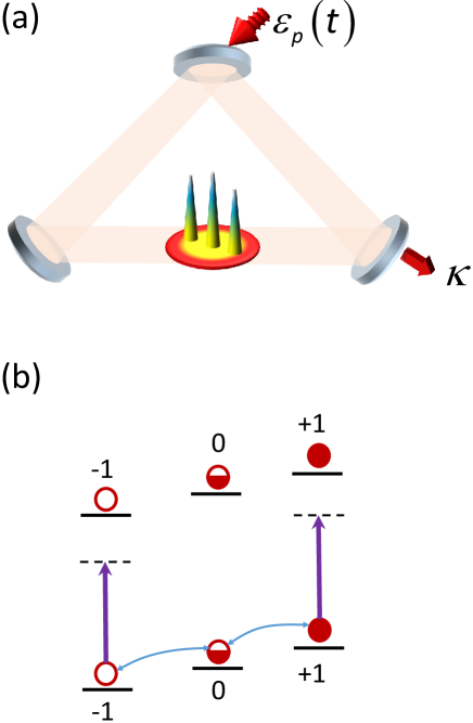
Figure 1: Schematic diagram for generating cavity-amplified parametric resonance. (a) An $F=1$ spinor condensate is trapped inside a ring cavity. The cavity is coherently driven by an external laser with time-dependent amplitude $\varepsilon_{p}\left(t\right)$ and decays with a rate $\kappa$. (b) The cavity field is $\pi$-polarized and is dispersively coupled to the atomic system. In the meanwhile the spin-dependent collisions will lead to population transfer among the three spin components.

For the present system we apply single-mode approximation (SMA), under which all three atomic spin states are described by the same spatial wavefunction $\psi\left(\mathbf{r}\right)$. SMA is appropriate for a condensate whose size is smaller than the spin healing length $\xi_{s}=h/\sqrt{2m_{a}\left|c_{2}\right|n}$ ($n$ is the atomic density). The case beyond SMA and with unbiased driving field was considered in our model2 .

After adiabatically eliminating the excited atomic level, the atom-cavity system can be described by the following Hamiltonian in a rotating frame with $\hbar=1$:

$$\hat{H}=\hat{H}_{0}+\left[U_{0}\left(\hat{c}_{+}^{\dagger}\hat{c}_{+}+\hat{c}_{-}^{\dagger}\hat{c}_{-}\right)-\delta_{c}\right]\hat{a}^{\dagger}\hat{a}+i\varepsilon_{p}\left(t\right)\left(\hat{a}^{\dagger}-\hat{a}\right)$$ (2)

where $U_{0}$ characterizes the strength of atom-photon coupling and $\delta_{c}=\omega_{p}-\omega_{c}$ is the cavity-pump detuning. $\hat{H}_{0}$ describes the dynamics of the spinor condensate spinor condensate ; hanPRL1998 and is given by

$$\hat{H}_{0}=\frac{\lambda}{N}\hat{c}_{a}^{\dagger}\hat{c}_{a^{\prime}}^{\dagger}\mathbf{F}_{ab}\cdot\mathbf{F}_{a^{\prime}b^{\prime}}\hat{c}_{b}\hat{c}_{b^{\prime}}$$ (3)

with $\lambda=Nc_{2}\int d\mathbf{r}\left|\psi\left(\mathbf{r}\right)\right|^{4}/2$. Here, the total particle number $N=\sum_{s}N_{s}$ is a constant-of-motion, $\hat{c}_{s}$ ($\hat{c}_{s}^{\dagger}$) is the bosonic annihilation (creation) operator of the atomic spin-$s$ ($s=0,\pm 1$) state, and the indices $a$, $a^{\prime}$, $b$, $b^{\prime}$ are summed over the spins. $\mathbf{F}$ are spin-1 matrices with

$$F_{x} =\frac{1}{\sqrt{2}}\left(\begin{array}[c]{ccc}0&1&0\\ 1&0&1\\ 0&1&0\end{array}\right)\text{, }F_{y}=\frac{i}{\sqrt{2}}\left(\begin{array}[c]{ccc}0&-1&0\\ 1&0&-1\\ 0&1&0\end{array}\right),$$ (10)

$$F_{z} =\left(\begin{array}[c]{ccc}1&0&0\\ 0&0&0\\ 0&0&-1\end{array}\right).$$ (14)

The evolution of the cavity-spinor BEC system can be described by the master equation

$$\frac{d\hat{\rho}}{dt}=-i\left[\hat{H},\hat{\rho}\right]+\kappa\left(2\hat{a}\hat{\rho}\hat{a}^{\dagger}-\hat{a}^{\dagger}\hat{a}\hat{\rho}-\hat{\rho}\hat{a}^{\dagger}\hat{a}\right),$$ (15)

with $\hat{\rho}$ denoting the total density operator for the atomic spin and cavity degrees of freedom.

The mean-field equations of motion for the $\mathcal{C}$-numbers $\alpha=\left\langle\hat{a}\right\rangle$ and $\left\langle\hat{c}_{s}\right\rangle=\sqrt{N\rho_{s}}\exp\left(-i\theta_{s}\right)$ ($\rho_{s}$ is the population normalized with respect to the total atom number $N$ while $\theta_{s}$ is the corresponding phase) can then be derived from the master equation (15) as

$$\dot{\alpha} =\left[i\delta_{c}-iU_{0}N\left(1-\rho_{0}\right)-\kappa\right]\alpha+\varepsilon_{p}\left(t\right),$$ (16a)

$$\dot{\rho}_{0} =2\lambda\rho_{0}\sqrt{\left(1-\rho_{0}\right)^{2}-m^{2}}\sin\theta,$$ (16b)

$$\dot{\theta} =-2U_{0}\left|\alpha\right|^{2}+2\lambda$$

$$\times\left[1-2\rho_{0}+\frac{\left(1-\rho_{0}\right)\left(1-2\rho_{0}\right)-m^{2}}{\sqrt{\left(1-\rho_{0}\right)^{2}-m^{2}}}\cos\theta\right],$$ (16c)

where $$\theta=2\theta_{0}-\theta_{+}-\theta_{-} m=\rho_{+}-\rho_{-} \cdot t m=0$$ is the relative phase, and the magnetization. Here means derivative with respect to time . For simplicity we assume zero magnetization in the following discussion.

At this point we specify the parameters used in the present work: For spinor ⁸⁷Rb condensate considered in chapmanNC2016 , $\lambda=-2\pi\times 14$ Hz and $N=4\times 10^{4}$, for typical cavity setup we assume that $\kappa=2\pi\times 1$ MHz, $U_{0}=-2\pi\times 10$ Hz, $\varepsilon_{0}=4\kappa$ and $f_{0}=0.1$. By considering the fact that the cavity decay rate $\kappa$ is typically much larger than both the frequency of atomic spin oscillation (characterized by the intrinsic frequency $\lambda$) and the modulation frequency $\omega_{m}$ (around hundreds Hz as we will show below), we can adiabatically eliminate $\alpha$ from Eq. (16a) and replace $\alpha$ in Eq. (16c) with

$$\alpha\left(t\right)\approx\frac{\varepsilon_{p}\left(t\right)}{\kappa-i\delta_{c}+iU_{0}N\left(1-\rho_{0}\right)}.$$ (17)

Thus $\left|\alpha\left(t\right)\right|^{2}\approx\left|\alpha_{0}\right|^{2}\left[1+2f_{0}\sin\left(\omega_{m}t\right)\right]$ with $\alpha_{0}=\varepsilon_{0}/\left[\kappa-i\delta_{c}+iU_{0}N\left(1-\rho_{0}\right)\right]$, where we have kept only the lowest order in $f_{0}$ by considering weak driving.

By introducing $\theta\left(t\right)=\phi\left(t\right)+z\cos\left(\omega_{m}t\right)$ with $z=2\omega_{0}f_{0}/\omega_{m}$ and $\omega_{0}=2U_{0}\left|\alpha_{0}\right|^{2}$, Eqs. (16b) and (16c) become

$$\dot{\rho}_{0} =2\lambda\rho_{0}\left(1-\rho_{0}\right)\sum_{n=-\infty}^{\infty}J_{n}\left(z\right)\sin\left[\phi+n\left(\omega_{m}t+\frac{\pi}{2}\right)\right],$$

$$\dot{\phi} =-\omega_{0}+2\lambda\left(1-2\rho_{0}\right)\left\{1\right.$$

$$\left.+\sum_{n=-\infty}^{\infty}J_{n}\left(z\right)\cos\left[\phi+n\left(\omega_{m}t+\frac{\pi}{2}\right)\right]\right\},$$ (18)

where we have implicitly assumed that for evolution at high field with relatively large $\left|\omega_{0}/\lambda\right|$ the system is in the Zeeman energy dominated regime in which the oscillation dynamics are suppressed, and consequently $\rho_{0}$ and $z$ can be assumed to be approximately constant chapmanNC2016 . Note also that the Jacobi-Anger expansions

$$\cos\left(z\cos\varphi\right) =\sum_{n=-\infty}^{\infty}J_{n}\left(z\right)\cos\left[n\left(\varphi+\frac{\pi}{2}\right)\right],$$

$$\sin\left(z\cos\varphi\right) =\sum_{n=-\infty}^{\infty}J_{n}\left(z\right)\sin\left[n\left(\varphi+\frac{\pi}{2}\right)\right]$$ (19)

have been used in deriving Eqs. (18), where $J_{n}\left(z\right)$ is the $n$th-order Bessel function of the first kind.

Replacing $\phi\rightarrow\phi-n\left(\omega_{m}t+\pi/2\right)$, one can see that only at some specific values of $n=k$ with $k\omega_{m}\sim\omega_{0}$ the value of $\phi$ does not monotonically depend on $t$, i.e., yielding nonzero time average of $\dot{\rho}_{0}$. Around these specific values of $k$ giving rise to parametric resonances, Eqs. (18) resort to

$$\dot{\rho}_{0} =2\lambda\eta_{k}\rho_{0}\left(1-\rho_{0}\right)\sin\phi,$$

$$\dot{\phi} =\delta_{k}+2\lambda\left(1-2\rho_{0}\right)\left(1+\eta_{k}\cos\phi\right),$$ (20)

where $\eta_{k}=J_{k}\left(z\right)$ and $\delta_{k}=k\omega_{m}-\omega_{0}$. The equations-of-motion (20) have similar form as the secular equations derived in gerbier2018 . However one should notice that $\delta_{k}$ relates to $\left|\alpha_{0}\right|^{2}$ and thus is a complex function of $\rho_{0}$, which introduces nonlinearity into the system.

To illustrate the dynamical properties near parametric resonance, one can use $\dot{\rho_{0}}=-2\partial H_{k}/\partial\phi$ and $\dot{\phi}=2\partial H_{k}/\partial\rho_{0}$ to construct, in terms of two conjugate variables $\rho_{0}$ and $\phi$, the following mean-field Hamiltonian $H_{k}$:

$$H_{k}=\lambda\rho_{0}\left(1-\rho_{0}\right)\left(1+\eta_{k}\cos\phi\right)+U_{k}\left(\rho_{0}\right),$$ (21)

where

$$U_{k}\left(\rho_{0}\right)=\frac{k\omega_{m}}{2}\rho_{0}+\frac{\varepsilon_{0}^{2}}{N\kappa}\arctan\left[\frac{NU_{0}}{\kappa}\left(1-\rho_{0}\right)-\frac{\delta_{c}}{\kappa}\right]$$ (22)

represents the cavity-mediated atom-atom interaction.

III cavity-amplified parametric resonance

We first consider the cavity-free case where in Eqs. (16) $U_{0}\left|\alpha\right|^{2}$ represents a quadratic Zeeman shift independent of $\rho_{0}$, then $U_{k}\left(\rho_{0}\right)$ in Eq. (22) resorts to $\delta_{k}\rho_{0}/2$. If the periodic modulation is not applied ($f_{0}=0$) one can estimate that $\left|U_{0}\left|\alpha\right|^{2}/\lambda\right|\approx 11.4$ at $\delta_{c}=0$. One can further show that zhangPRA2005 , under this high field the maximum oscillation amplitude for $\rho_{0}$ is approximately $0.02$ when $\rho_{0}\left(0\right)=0.5$ and goes to zero when $\rho_{0}\left(0\right)=0$ or $1$. When one approaches the $k$-th parametric resonance with the periodic modulation applied, we can make use of Eq. (21) and rewrite Eqs. (20) as

$$\left(\dot{\rho}_{0}\right)^{2} =4\lambda^{2}\rho_{0}^{2}\left(1-\rho_{0}\right)^{2}\left\{\eta_{k}^{2}-\left[\frac{H_{k}\left(\rho_{0}\left(0\right),\phi\left(0\right)\right)}{\lambda\rho_{0}\left(1-\rho_{0}\right)}\right.\right.$$

$$\left.\left.-\frac{\delta_{k}}{2\lambda\left(1-\rho_{0}\right)}-1\right]^{2}\right\}.$$ (23)

Eq. (23) typically represents undamped cubic anharmonic oscillator whose analytical solution can generally be written in the form of Jacobi elliptic functions.

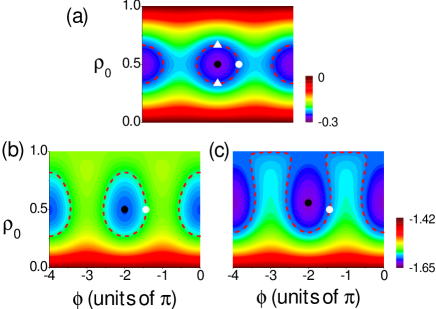
Figure 2: Phase-space contour plot of $H_{k}$ (in unit of $\left|\lambda\right|$) at $k=-1$ resonance. (a) Cavity-free case with $\delta_{k}=0$. The case incoporating cavity backaction are shown in (b) $\delta_{k}=0$ and (c) $\delta_{k}=0.09\lambda$ with $\delta_{c}=-0.35\kappa$. The red-dashed lines refer to the contour determined by the initial state of the system. The white dots refer to the initial state of the system, while the black dots refer to equilibrium position and the white triangles refer to the states when the system passing through the equilibrium position in the pendulum analogy.

Physical insights into the oscillation properties can be obtained via the phase-space contour plot of $H_{k}$. We assume that the spinor condensate is initially prepared in a state with $\rho_{0}\left(0\right)=0.5$ and $\theta\left(0\right)=-\pi$ (corresponding to an effective large negative quadratic Zeeman energy as compared with chapmanNC2016 in which the initial state is $\theta\left(0\right)=\pi$ with a large positive quadratic Zeeman energy, $\phi\left(0\right)=\theta\left(0\right)-z+k\pi/2$). When the driving frequency $\omega_{m}$ is appropriately tuned to the $k=-1$ resonance with $\delta_{k=-1}=0$, the equal-$H_{-1}$ contour diagram in the phase space defined by the conjugate pair $\left(\phi,\rho_{0}\right)$ is plotted in Fig. 2(a). The contour plot typically reproduces the phase diagram of a simple pendulum, indicating that the system evolves along a contour (marked as a red-dashed line) determined by its initial state (marked as a white dot). The center of the contour (marked as a black dot) represents the equilibrium position in the pendulum analogy, which is a stable stationary solution of Eqs. (20) (the dynamical properties of the stationary solutions can be studied via the standard linear stability analysis). The two points marked as white triangles are two real stationary solutions of Eq. (23) located in the region $\rho_{0}\in\left[0,1\right]$, symbolizing a pendulum passing through its equilibrium position with maximum speed from different direction. Their difference is the oscillation amplitude taking the value around $0.33$.

When the cavity backaction is taken into account, one should notice that the value of $\delta_{k}$ is implicitly $\rho_{0}$-dependent. We first assume that the driving frequency $\omega_{m}$ is appropriately tuned to $\delta_{k=-1}=0$ with respect to the initial state of $\rho_{0}\left(0\right)=0.5$ and $\theta\left(0\right)=-\pi$, and the corresponding phase diagram is shown in Fig. 2(b). Although the contour plot still captures the main features of a pendulum, its topology changes as compared with Fig. 2(a). In this case one cannot find stationary solutions of Eq. (23) in the $\rho_{0}\in\left[0,1\right]$ region, implying a non-rigid pendulum. The oscillation amplitude is estimated to take the value of $0.55$, which is much larger than that of the cavity-free case. If $\omega_{m}$ is tuned slightly deviate from the resonance with $\delta_{k=-1}=0.09\lambda$, as shown in Fig. 2(c), the red-dashed line changes its topology from a closed to an open line, and in the pendulum analogy it signals that the pendulum swings all the way over the vertical upright position and continues with the same direction of swing. In this case the oscillation amplitude has the maximum value of about $0.7$, doubles as compared to the cavity-free case. A drastic topology change is usually associated with additional fixed points (more than $1$ at $\phi=n\pi$), which can be determined from the stationary solutions of Eqs. (20). From numerical simulations we find that for the $k=-1$ resonance additional fixed points appear in the region $\delta_{c}\in\left[-0.24\text{, }-0.68\right]\kappa$ for the present parameter setup, indicating that one can seek parametric resonance amplification in this parameter region.

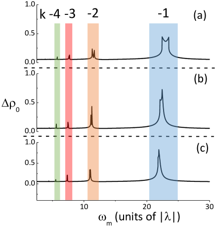
Figure 3: Oscillation amplitude $\Delta\rho_{0}$ versus modulation frequency $\omega_{m}$ (in unit of $\left|\lambda\right|$) for (a) cavity-free case and the cases with cavity backaction at (b) $\delta_{c}=-0.35\kappa$; (c) $\delta_{c}=-0.4\kappa$. The numbered color zone indicates the parametric region in which the $k$-th order resonance is excited.

A sketch of cavity-mediated parametric resonance is presented in Fig. 3 via numerical simulations of Eqs. (16), in which the regions of different $k$-th order resonances (from $k=-1$ to $-4$) can be well identified. Since $\omega_{0}<0$ (due to $U_{0}<0$), on parametric resonances $k$ should take negative values. One can notice that the oscillation amplitude $\Delta\rho_{0}$ significantly decreases for higher $\left|k\right|$-th order resonance and those resonances beyond $k=-4$ are not marked as the oscillation amplitudes are too small to be unambiguously distinguished from those not excited. This can be traced to the coupling coefficient $\eta_{k}=J_{k}\left(z\right)=J_{k}\left(2\omega_{0}f_{0}/\omega_{m}\right)\sim J_{k}\left(k/5\right)$, from which one can estimate that the value of $\eta_{k}$ decays from $10^{-1}$ to $10^{-4}$ when $k$ varies from $-1$ to $-5$. This indicates that high-$\left|k\right|$-th order parametric resonances are much less likely to be excited. In the pendulum analogy it corresponds to the case that the system evolves along an ellipse with large curvature, i.e., the pendulum velocity is small while passing through the equilibrium position.

On resonance the oscillation amplitude $\Delta\rho_{0}$ can display a typical two-peak structure, as can be seen from the $k=-1$ and $-2$ resonances for the cavity-free case shown in Fig. 3(a). The exact resonance point $\omega_{m}=\omega_{0}/k$ locates in the middle of the two peaks, which is also demonstrated in experiment gerbier2018 . In experiment chapmanNC2016 population $\rho_{0}$ are measured after $100$ ms of parametric excitation and near the lowest-order resonance population $\rho_{0}$ behave as a sinusoidal function of $\omega_{m}$ with the resonance point on the node, which also supports our predictions here. The peaks signal the critical points at which the pendulum possesses enough energy to pass through the top position, and they also represent dynamical phase transitions of the system from $\phi$-running modes to $\phi$-$\pi$ modes. Cavity-induced nonlinearity substantially modifies the topology of the phase diagram and as such the two peaks merge into one, as shown in Fig. 3(b) and (c).

More importantly, through cavity-mediated parametric excitation the oscillation amplitude $\Delta\rho_{0}$ can be significantly amplified. For the lowest $k=-1$ resonance, Fig. 3 demonstrates that cavity backaction can amplify the oscillation amplitude to the value of $0.83$ as compared with $0.45$ in the cavity-free case. For high-order resonances such as $k=-3$, $\Delta\rho_{0}$ can still be amplified to $0.21$ as compared with the cavity-free value of $0.13$. These results suggest that cavity backaction can not only make the low-order parametric resonances more prominent, but also can make the detection of the original weak high-order resonances easier.

IV measurement discussion

In experiments chapmanNC2016 ; gerbier2018 spin dynamics are probed via Stern-Gerlach imaging, which performs fluorescence detection or absorption imaging after a time-of-flight of spinor condensate in a magnetic field gradient separating the different spin components. The condensate is destructed after each detection, which means one will have to repeat the experiment many times to measure the dynamics. Since the intracavity photon number $\left|\alpha\right|^{2}$ relates to the normalized spin population $\rho_{0}$ as can be seen from Eq. (17), this indicates that it can be used for observing real-time evolution of spin dynamics.

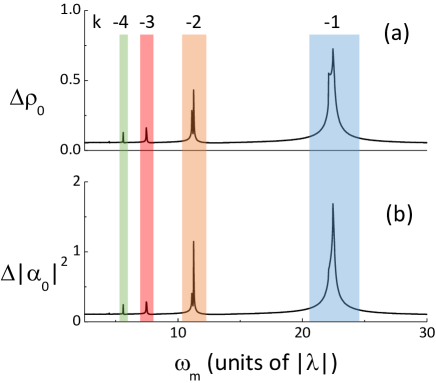
Figure 4: (a) Oscillation amplitude $\Delta\rho_{0}$ and (b) the corresponding cavity oscillation amplitude $\Delta\left|\alpha_{0}\right|^{2}$ versus modulation frequency $\omega_{m}$ (in unit of $\left|\lambda\right|$) at $\delta_{c}=-0.35\kappa$.

As $\left|\alpha\left(t\right)\right|^{2}\approx\left|\alpha_{0}\right|^{2}\left[1+2f_{0}\sin\left(\omega_{m}t\right)\right]$, one can integrate $\left|\alpha\left(t\right)\right|^{2}$ over several periods of modulation to eliminate the high-frequency oscillation while during this relatively short time (compared to the oscillation period) the value of $\left|\alpha_{0}\right|^{2}$ is roughly unchanged. In Fig. 4 we plot the oscillation amplitude of spin population $\Delta\rho_{0}$ as well as that of averaged intracavity photon number $\Delta\left|\alpha_{0}\right|^{2}$, the results indicate that continuous observation of spin dynamics can be realized via measuring the corresponding averaged intracavity photon number $\left|\alpha_{0}\right|^{2}$. Parametric resonances can also be well identified. We note that the idea of probing spin dynamics with cavity transmission spectra was also proposed in zhangPRA2009 .

V summary and outlook

It is interesting to note that bistability in spin-1 condensate was found in gerbier2018 , which is aroused by the dissipation of spinor condensate and hysteresis (usually associated with bistability) was observed for long evolution times. In the present work we concentrate on relatively short-time dynamics in which spin relaxation will not play a significant role. However we would like to note that the interplay between the atomic spin mixing and the cavity light field can lead to a strong matter-wave nonlinearity and bistability, which has been demonstrated in previous works our model ; our model2 . So certainly one can expect that bistability will take place with parametric excitations here even for short times at appropriate conditions.

In summary we have studied nonlinear Floquet dynamics of spinor condensate in an optical cavity. Floquet driving leads to parametric resonance while the cavity-induced nonlinearity makes it amplified. Since the order of observable resonances is limited by the maximum quadratic Zeeman energy (maximal magnetic field) achievable chapmanNC2016 ; gerbier2018 , thus the scheme propsed in the present work provide a way to experimentally probe high-order parametric resonances without the request of increasing the quadratic Zeeman energy. Feasibility of real-time observation of spin dynamics via cavity output is also discussed. Other interesting phenomena in this system which can be modified via the coupling to the cavity, such as quantum spin squeezing chapmanNP2012 , entanglement youexperiment ; massonPRL2019 ; gil as well as phase transition floquet spinor , will be left for further investigation. It is also interesting to note that a quite recent work clarkNature2019 demonstrated ”Floquet polaritons” via the coupling of Floquet modulated ⁸⁷Rb atoms with cavity light modes.

- (1) J. H. Shirley, Phys. Rev. 138, B979 (1965).
- (2) W. R. Salzman, Phys. Rev. A 10, 461 (1974).
- (3) J. Henkel and M. Holthaus, Phys. Rev. A 45, 1978 (1992); K. Dietz, J. Henkel, and M. Holthaus, Phys. Rev. A 45, 4960 (1992); H. P. Breuer, K. Dietz, and M. Holthaus, Phys. Rev. A 47, 725 (1993).
- (4) N. Goldman and J. Dalibard, Phys. Rev. X 4, 031027 (2014) and references therein.
- (5) L. W. Clark, A. Gaj, L. Feng, and C. Chin, Nature 551, 356 (2017).
- (6) L. Feng, J. Hu, L. W. Clark, and C. Chin, Science 363, 521 (2019).
- (7) M. Holthaus, J. Phys. B 49, 013001 (2016).
- (8) C. J. Fujiwara, K. Singh, Z. A. Geiger, R. Senaratne, S. V. Rajagopal, M. Lipatov, and D. M. Weld, Phys. Rev. Lett. 122, 010402 (2019).
- (9) P. Plötz, J. Madroñero and S. Wimberger, J. Phys. B 43, 081001 (2010); P. Plötz and S. Wimberger, Eur. Phys. J. D 65, 199 (2011); C. A. Parra-Murillo, J. Madroñero, and S. Wimberger, Phys. Rev. A 88, 032119 (2013).
- (10) S. Smirnov, D. Bercioux, M. Grifoni, and K. Richter, Phys. Rev. Lett. 100, 230601 (2008); M. Scheid, A. Pfund, D. Bercioux, and K. Richter, Phys. Rev. B 76, 195303 (2007); S. Smirnov, D. Bercioux, M. Grifoni, and K. Richter, Phys. Rev. B 78, 245323 (2008).
- (11) M. Grifoni, M. S. Ferreira, J. Peguiron, and J. B. Majer, Phys. Rev. Lett. 89, 146801 (2002).
- (12) C. E. Creffield, Phys. Rev. Lett. 99, 110501 (2007); M. Heimsoth, C. E. Creffield, and F. Sols, Phys. Rev. A 82, 023607 (2010).
- (13) E. Lundh and M. Wallin, Phys. Rev. Lett. 94, 110603 (2005).
- (14) C.-C. Chien and M. Di Ventra, Phys. Rev. A 87, 023609 (2013).
- (15) I. Dana, V. Ramareddy, I. Talukdar, and G. S. Summy, Phys. Rev. Lett. 100, 024103 (2008); R. K. Shrestha, J. Ni, W. K. Lam, G. S. Summy, and S. Wimberger, Phys. Rev. E 88, 034901 (2013); J. Ni, W. K. Lam, S. Dadras, M. F. Borunda, S. Wimberger, and G. S. Summy, Phys. Rev. A 94, 043620 (2016); J. Ni, S. Dadras, W. K. Lam, R. K. Shrestha, M. Sadgrove, S. Wimberger, and G. S. Summy, Ann. Phys. 529, 1600335 (2017).
- (16) M. Sadgrove, M. Horikoshi, T. Sekimura, and K. Nakagawa, Phys. Rev. Lett. 99, 043002 (2007).
- (17) M. Glück, A. R. Kolovsky, and H. J. Korsch, Phys. Rev. Lett. 82, 1534 (1999); Phys. Rev. E 60, 247 (1999); M. Glück, M. Hankel, A. R. Kolovsky, and H. J. Korsch, Phys. Rev. A 61, 061402(R) (2000); S. Wimberger, R. Mannella, O. Morsch, E. Arimondo, A. R. Kolovsky, and A. Buchleitner, Phys. Rev. A 72, 063610 (2005).
- (18) A. Eckardt, Rev. Mod. Phys. 89, 011004 (2017).
- (19) C. Wu, J. Fan, G. Chen, and S. Jia, Phys. Rev. A 99, 013617 (2019).
- (20) M. Weiß, C. Groiseau, W. K. Lam, R. Burioni, A. Vezzani, G. S. Summy, and S. Wimberger, Phys. Rev. A 92, 033606 (2015); G. Summy and S. Wimberger, Phys. Rev. A 93, 023638 (2016).
- (21) D. V. Else, B. Bauer, and C. Nayak, Phys. Rev. Lett. 117, 090402 (2016).
- (22) B. Huang, Y.-H. Wu, and W. V. Liu, Phys. Rev. Lett. 120, 110603 (2018).
- (23) X.-F. Zhou, C. Wu, G.-C. Guo, R. Wang, H. Pu, and Z.-W. Zhou, Phys. Rev. Lett. 120, 130402 (2018); J.-M. Cheng, M. Gong, G.-C. Guo, Z.-W. Zhou, and X.-F. Zhou, arXiv:1907.02216.
- (24) T. M. Hoang, M. Anquez, B. A. Robbins, X. Y. Yang, B. J. Land, C. D. Hamley, and M. S. Chapman, Nat. Comm. 7, 11233 (2016).
- (25) B. Evrard, A. Qu, K. Jiménez-García, J. Dalibard, F. Gerbier, Phys. Rev. A 100, 023604 (2019).
- (26) S. Dadras, A. Gresch, C. Groiseau, S. Wimberger, and G. S. Summy, Phys. Rev. Lett. 121, 070402 (2018); Phys. Rev. A 99, 043617 (2019).
- (27) J. Stenger, S. Inouye, D. M. Stamper-Kurn, H.-J. Miesner, A. P. Chikkatur, and W. Ketterle, Nature 396, 345 (1998).
- (28) T.-L. Ho, Phys. Rev. Lett. 81, 742 (1998); T. Ohmi and K. Machida, J. Phys. Soc. Jpn. 67, 1822 (1998).
- (29) Y. Kawaguchi and M. Ueda, Phys. Rep. 520, 253 (2012).
- (30) C. K. Law, H. Pu, and N. P. Bigelow, Phys. Rev. Lett. 81, 5257 (1998).
- (31) M.-S. Chang, Q. Qin, W. Zhang, L. You, and M. S. Chapman, Nat. Phys. 1, 111 (2005).
- (32) A. T. Black, E. Gomez, L. D. Turner, S. Jung, and P. D. Lett, Phys. Rev. Lett. 99, 070403 (2007); Y. Liu, S. Jung, S. E. Maxwell, L. D. Turner, E. Tiesinga, and P. D. Lett, Phys. Rev. Lett. 102, 125301 (2009).
- (33) W. Zhang, D. L. Zhou, M.-S. Chang, M. S. Chapman, and L. You, Phys. Rev. A 72, 013602 (2005).
- (34) A. Widera, F. Gerbier, S. Fölling, T. Gericke, O. Mandel, and I. Bloch, Phys. Rev. Lett. 95, 190405 (2005).
- (35) D. Jacob, L. Shao, V. Corre, T. Zibold, L. D. Sarlo, E. Mimoun, J. Dalibard, and F. Gerbier, Phys. Rev. A 86, 061601(R) (2012).
- (36) J. Kronjäger, C. Becker, P. Navez, K. Bongs, and K. Sengstock, Phys. Rev. Lett. 97, 110404 (2006).
- (37) S. W. Seo, W. J. Kwon, S. Kang, and Y. Shin, Phys. Rev. Lett. 116, 185301 (2016).
- (38) Q. Xie and W. Hai, Phys. Rev. A 80, 053603 (2009).
- (39) H. L. Haroutyunyan and G. Nienhuis, Phys. Rev. A 70, 063603 (2004).
- (40) S. Choi and N. P. Bigelow, Phys. Rev. A 72, 033612 (2005).
- (41) A. Eckardt, T. Jinasundera, C. Weiss, and M. Holthaus, Phys. Rev. Lett. 95, 200401 (2005).
- (42) G.-F. Wang, L.-B. Fu, and J. Liu, Phys. Rev. A 73, 013619 (2006).
- (43) L.-M. Kuang and Z.-W. Ouyang, Phys. Rev. A 61, 023604 (2000).
- (44) S. Ashhab, J. R. Johansson, A. M. Zagoskin, and F. Nori, Phys. Rev. A 75, 063414 (2007).
- (45) H. Ritsch, P. Domokos, F. Brennecke, and T. Esslinger, Rev. Mod. Phys. 85, 553 (2013) and references therein.
- (46) M. A. Norcia, R. J. Lewis-Swan, J. R. K. Cline, B. Zhu, A. M. Rey, and J. K. Thompson, Science 361, 259 (2018).
- (47) E. J. Davis, G. Bentsen, L. Homeier, T. Li, and M. H. Schleier-Smith, Phys. Rev. Lett. 122, 010405 (2019).
- (48) M. Landini, N. Dogra, K. Kroeger, L. Hruby, T. Donner, and T. Esslinger, Phys. Rev. Lett. 120, 223602 (2018).
- (49) R. M. Kroeze, Y. Guo, V. D. Vaidya, J. Keeling, and B. L. Lev, Phys. Rev. Lett. 121, 163601 (2018).
- (50) J. Larson, B. Damski, G. Morigi, and M. Lewenstein, Phys. Rev. Lett. 100, 050401 (2008); J. Larson, S. Fernádez-Vidal, G. Morigi, and M. Lewenstein, New J. Phys. 10, 045002 (2008).
- (51) J.-N. Wu, J. Qian, X.-D. Zhao, L. Zhou, and W. Zhang, Phys. Rev. A 88, 065601 (2013).
- (52) J. Goldwin, B. P. Venkatesh, and D. H. J. O’Dell, Phys. Rev. Lett. 113, 073003 (2014).
- (53) L. Dong, L. Zhou, B. Wu, B. Ramachandhran, and H. Pu, Phys. Rev. A 89, 011602(R) (2014).
- (54) Y. Deng, J. Cheng, H. Jing, and S. Yi, Phys. Rev. Lett. 112, 143007 (2014).
- (55) L. Santos, M. Fattori, J. Stuhler, and T. Pfau, Phys. Rev. A 75, 053606 (2007).
- (56) X.-W. Luo and C. Zhang, Phys. Rev. Lett. 120, 263202 (2018).
- (57) J. G. Cosme, C. Georges, A. Hemmerich, and L. Mathey, Phys. Rev. Lett. 121, 153001 (2018).
- (58) B. Megyeri, G. Harvie, A. Lampis, and J. Goldwin, Phys. Rev. Lett. 121, 163603 (2018).
- (59) S. C. Schuster, P. Wolf, D. Schmidt, S. Slama, and C. Zimmermann, Phys. Rev. Lett. 121, 223601 (2018).
- (60) L. Zhou, H. Pu, H. Y. Ling, K. Zhang, and W. Zhang, Phys. Rev. A 81, 063641 (2010).
- (61) J. M. Zhang, S. Cui, H. Jing, D. L. Zhou, and W. M. Liu, Phys. Rev. A 80, 043623 (2009).
- (62) L. Zhou, H. Pu, H. Y. Ling, and W. Zhang, Phys. Rev. Lett. 103, 160403 (2009).
- (63) C. D. Hamley, C. S. Gerving, T. M. Hoang, E. M. Bookjans, and M. S. Chapman, Nat. Phys. 8, 305 (2012).
- (64) Stuart J. Masson and Scott Parkins, Phys. Rev. Lett. 122, 103601 (2019).
- (65) X.-Y. Luo, Y.-Q. Zou,, L.-N. Wu, Q. Liu, M.-F. Han, M. K. Tey, and L. You, Science 355, 620 (2017); Y.-Q. Zou, L.-N. Wu, Q. Liu, X.-Y. Luo, S.-F. Guo, J.-H. Cao, M. K. Tey, and L. You, Proc. Natl. Acad. Sci. U.S.A. 115, 6381 (2018).
- (66) K. Fujimoto and S. Uchino, arXiv:1901.09386.
- (67) L. W. Clark, N. Jia, N. Schine, C. Baum, A. Georgakopoulos, and J. Simon, Nature 571, 532 (2019).