Learning Sparse Nonparametric DAGs

Abstract

We develop a framework for learning sparse nonparametric directed acyclic graphs (DAGs) from data. Our approach is based on a recent algebraic characterization of DAGs that led to a fully continuous program for score-based learning of DAG models parametrized by a linear structural equation model (SEM). We extend this algebraic characterization to nonparametric SEM by leveraging nonparametric sparsity based on partial derivatives, resulting in a continuous optimization problem that can be applied to a variety of nonparametric and semiparametric models including GLMs, additive noise models, and index models as special cases. Unlike existing approaches that require specific modeling choices, loss functions, or algorithms, we present a completely general framework that can be applied to general nonlinear models (e.g. without additive noise), general differentiable loss functions, and generic black-box optimization routines. The code is available at https://github.com/xunzheng/notears.

1 Introduction

Learning DAGs from data is an important and classical problem in machine learning, with a diverse array of applications in causal inference (Spirtes et al., 2000), fairness and accountability (Kusner et al., 2017), medicine (Heckerman et al., 1992), and finance (Sanford and Moosa, 2012). In addition to their undirected counterparts, DAG models offer a parsimonious, interpretable representation of a joint distribution that is useful in practice. Unfortunately, existing methods for learning DAGs typically rely on specific model assumptions (e.g. linear or additive) and specialized algorithms (e.g. constraint-based or greedy optimization). As a result, the burden is on the user to choose amongst many possible models and algorithms, which requires significant expertise. Thus, there is a need for a general framework for learning different DAG models—subsuming, for example, linear, parametric, and nonparametric—that does not require specialized algorithms. Ideally, the problem could be formulated as a conventional optimization problem that can be tackled with general purpose solvers, much like the current state-of-the-art for undirected graphical models (e.g. Suggala et al., 2017; Yang et al., 2015; Liu et al., 2009; Hsieh et al., 2013; Banerjee et al., 2008).

In this paper, we develop such a general algorithmic framework for score-based learning of DAG models. This framework is flexible enough to learn general nonparametric dependence while also easily adapting to parametric and semiparametric models, including nonlinear models. The framework is based on a recent algebraic characterization of acyclicity due to Zheng et al. (2018) that recasts the score-based optimization problem as a continuous problem, instead of the traditional combinatorial approach. This allows generic optimization routines to be used in minimizing the score, providing a clean conceptual formulation of the problem that can be approached using any of the well-known algorithms from the optimization literature. This work relies heavily on the linear parametrization in terms of a weighted adjacency matrix $W\in\mathbb{R}^{d\times d}$, which is a stringent restriction on the class of models. One of the key technical contributions of the current work is extending this to general nonparametric problems, where no such parametrization in terms of a weighted adjacency matrix exists.

Contributions

Our main contributions can be summarized as follows:

• We develop a generic optimization problem that can be applied to nonlinear and nonparametric SEM and discuss various special cases including additive models and index models. In contrast to existing work, we show how this optimization problem can be solved to stationarity with generic solvers, eliminating the necessity for specialized algorithms and models.

• We extend the existing smooth characterization of acyclicity from Zheng et al. (2018) to general nonparametric models, show that the linear parametrization is a special case of the general framework, and apply this to several popular examples for modeling nonlinear dependencies (Section 3).

• We consider in detail two classes of nonparametric estimators defined through 1) Neural networks and 2) Orthogonal basis expansions, and study their properties (Section 4).

• We run extensive empirical evaluations on a variety of nonparametric and semiparametric models against recent state-of-the-art methods in order to demonstrate the effectiveness and generality of our framework (Section 5).

As with all score-based approaches to learning DAGs, ours relies on a nonconvex optimization problem. Despite this, we show that off-the-shelf solvers return stationary points that outperform other state-of-the-art methods. Finally, the algorithm itself can be implemented in standard machine learning libraries such as PyTorch, which should help the community to extend our approach to richer models moving forward.

Related work

The problem of learning nonlinear and nonparametric DAGs from data has generated significant interest in recent years, including additive models (Bühlmann et al., 2014; Voorman et al., 2014; Ernest et al., 2016), generalized linear models (Park, 2018; Park and Raskutti, 2017; Park and Park, 2019; Gu et al., 2018), additive noise models (Hoyer et al., 2009; Peters et al., 2014; Blöbaum et al., 2018; Mooij et al., 2016), post-nonlinear models (Zhang and Hyvärinen, 2009; Zhang et al., 2016) and general nonlinear SEM (Monti et al., 2019; Goudet et al., 2018; Kalainathan et al., 2018; Sgouritsa et al., 2015). Recently, Yu et al. (2019) proposed to use graph neural networks for nonlinear measurement models and Huang et al. (2018) proposed a generalized score function for general SEM. The latter work is based on recent work in kernel-based measures of dependence (Gretton et al., 2005; Fukumizu et al., 2008; Zhang et al., 2012). Another line of work uses quantile scoring (Tagasovska et al., 2018). Also of relevance is the literature on nonparametric variable selection (Bertin et al., 2008; Lafferty et al., 2008; Miller et al., 2010; Rosasco et al., 2013; Gregorová et al., 2018) and approaches based on neural networks (Feng and Simon, 2017; Ye and Sun, 2018; Abid et al., 2019). The main distinction between our work and previous work is that our framework is not tied to a specific model—as in Yu et al. (2019); Bühlmann et al. (2014); Park (2018)—as our focus is on a generic formulation of an optimization problem that can be solved with generic solvers (see Section 2 for a more detailed comparison). This also distinguishes this paper from concurrent work by Lachapelle et al. (2019) that focuses on neural network-based nonlinearities in the local conditional probabilities. Furthermore, compared to Huang et al. (2018) and Yu et al. (2019), our approach can be much more efficient (Section 5.1; Appendix C). As such, we hope that this work is able to spur future work using more sophisticated nonparametric estimators and optimization schemes.

Notation

Norms will always be explicitly subscripted to avoid confusion: $\|\cdot\|_{p}$ is the $\ell_{p}$-norm on vectors, $\|\cdot\|_{L^{p}}$ is the $L^{p}$-norm on functions, $\|\cdot\|_{p,q}$ is the $(p,q)$-norm on matrices, and $\|\cdot\|_{F}=\|\cdot\|_{2,2}$ is the matrix Frobenius norm. For functions $f\mathrel{\mathop{\mathchar 58\relax}}\mathbb{R}^{s}\to\mathbb{R}$ and a matrix $A\in\mathbb{R}^{n\times s}$, we adopt the convention that $f(A)\in\mathbb{R}^{n}$ is the vector whose $i$th element is $f(a^{i})$, where $a^{i}$ is the $i$th row of $A$.

2 Background

Our approach is based on (acyclic) structural equation models as follows. Let $X=(X_{1},\ldots,X_{d})$ be a random vector and $\mathsf{G}=(\mathsf{V},\mathsf{E})$ a DAG with $\mathsf{V}=X$. We assume that there exist functions $f_{j}\mathrel{\mathop{\mathchar 58\relax}}\mathbb{R}^{d}\to\mathbb{R}$ and $g_{j}\mathrel{\mathop{\mathchar 58\relax}}\mathbb{R}\to\mathbb{R}$ such that

$$\mathbb{E}[X_{j}\,|\,X_{\operatorname{pa}(j)}]=g_{j}(f_{j}(X)),\quad\mathbb{E}f_{j}(X)=0$$ (1)

and $f_{j}(u_{1},\ldots,u_{d})$ does not depend on $u_{k}$ if $X_{k}\notin\operatorname{pa}(j)$, where $\operatorname{pa}(j)$ denotes the parents of $X_{j}$ in $\mathsf{G}$. Formally, the independence statement means that for any $X_{k}\notin\operatorname{pa}(j)$, the function $a(u)\mathrel{\mathop{\mathchar 58\relax}}=f_{j}(X_{1},\ldots,X_{k-1},u,X_{k+1},X_{d})$ is constant for all $u\in\mathbb{R}$. Thus, $\mathsf{G}$ encodes the conditional independence structure of $X$. The functions $g_{j}$, which are typically known, allow for possible non-additive errors such as in generalized linear models (GLMs). The model (1) is quite general and includes additive noise models, linear and generalized linear models, and additive models as special cases (Section 3.3).

In this setting, the DAG learning problem can be stated as follows: Given a data matrix $\mathbf{X}=[\mathbf{x}_{1}\,|\,\cdots\,|\,\mathbf{x}_{d}]\in\mathbb{R}^{n\times d}$ consisting of $n$ i.i.d. observations of the model (1), we seek to learn the DAG $\mathsf{G}(X)$ that encodes the dependency between the variables in $X$. Our approach is to learn $f=(f_{1},\ldots,f_{d})$ such that $\mathsf{G}(f)=\mathsf{G}(X)$ using a score-based approach. Given a loss function $\ell(y,\hat{y})$ such as least squares or the negative log-likelihood, we consider the following program:

$$\begin{aligned} \min_{f}\ L(f)\ \text{ subject to }\ \mathsf{G}(f)\in\mathsf{DAG},\\ \text{where}\quad L(f)=\frac{1}{n}\sum_{j=1}^{d}\ell(\mathbf{x}_{j},f_{j}(\mathbf{X})).\end{aligned}$$ (2)

There are two challenges in this formulation: 1) How to enforce the acyclicity constraint that $\mathsf{G}(f)\in\mathsf{DAG}$, and 2) How to enforce sparsity in the learned DAG $\mathsf{G}(f)$? Previous work using linear and generalized linear models rely on a parametric representation of $\mathsf{G}$ via a weighted adjacency matrix $W\in\mathbb{R}^{d\times d}$, which is no longer well-defined in the model (1). To address this, we develop a suitable surrogate of $W$ defined for general nonparametric models, to which we can apply the trace exponential regularizer from Zheng et al. (2018).

2.1 Identifiability

Existing papers approach this problem as follows: 1) Assume a specific model for (1), 2) Prove identifiability for this specific model, and 3) Develop a specialized algorithm for learning this specific model. By contrast, our approach is generic: We do not assume any particular model form or algorithm, and instead develop a general framework that applies to any model that is identifiable. By now, there is a well-catalogued list of identifiability results for various linear, parametric, and nonlinear models, which we review briefly below (see also Section 3.3).

When the model (1) holds, the graph $\mathsf{G}$ is not necessarily uniquely defined: A well-known example is when $X$ is jointly normally distributed, in which case the $f_{j}$ are linear functions, and where it can be shown that the graph $\mathsf{G}$ is not uniquely specified. Fortunately, it is known that this case is somewhat exceptional: Assuming additive noise, as long as the $f_{j}$ are linear with non-Gaussian errors (Kagan et al., 1973; Shimizu et al., 2006; Loh and Bühlmann, 2014) or the functions $f_{j}$ are nonlinear (Hoyer et al., 2009; Zhang and Hyvärinen, 2009; Peters et al., 2014), then the graph $\mathsf{G}$ is generally identifiable. We refer the reader to Peters et al. (2014) for details. Another example are so-called quadratic variance function models, which are parametric models that subsume many generalized linear models (Park and Raskutti, 2017; Park, 2018). In the sequel, we assume that the model is chosen such that the graph $\mathsf{G}$ is uniquely defined from (1), and this dependence will be emphasized by writing $\mathsf{G}=\mathsf{G}(X)$. Similarly, any collection of functions $f=(f_{1},\ldots,f_{d})$ defines a graph $\mathsf{G}(f)$ in the obvious way. See Section 3.3 for specific examples with discussion on identifiability.

2.2 Comparison to existing approaches

It is instructive at this point to highlight the main distinction between our approach and existing approaches. A common approach is to assume the $f_{j}$ are easily parametrized (e.g. linearity) (Zheng et al., 2018; Aragam and Zhou, 2015; Gu et al., 2018; Park and Raskutti, 2017; Park, 2018; Chen et al., 2018; Ghoshal and Honorio, 2017). In this case, one can easily encode the structure of $\mathsf{G}$ via, e.g. a weighted adjacency matrix, and learning $\mathsf{G}$ reduces to a parametric estimation problem. Nonparametric extensions of this approach include additive models (Bühlmann et al., 2014; Voorman et al., 2014), where the graph structure is easily deduced from the additive structure of the $f_{j}$. More recent work (Lachapelle et al., 2019; Yu et al., 2019) uses specific parametrizations via neural networks to encode $\mathsf{G}$. An alternative approach relies on exploiting the conditional independence structure of $X$, such as the post-nonlinear model (Zhang and Hyvärinen, 2009; Yu et al., 2019), the additive noise model (Peters et al., 2014), and kernel-based measures of conditional independence (Huang et al., 2018). Our framework can be viewed as a substantial generalization of these approaches: We use partial derivatives to measure dependence in the general nonparametric model (1) without assuming a particular form or parametrization, and do not explicitly require any of the machinery of nonparametric conditional independence (although we note in some places this machinery is implicit). This allows us to use nonparametric estimators such as multilayer perceptrons and basis expansions, for which these derivatives are easily computed. As a result, the score-based learning problem is reduced to an optimization problem that can be tackled using existing techniques, making our approach easily accessible.

3 Characterizing acyclicity in nonparametric SEM

In this section, we discuss how to extend the trace exponential regularizer from Zheng et al. (2018) beyond the linear setting, and then discuss several special cases.

3.1 Linear SEM and the trace exponential regularizer

We begin by briefly reviewing Zheng et al. (2018) in the linear case, i.e. $g_{j}(s)=s$ and $f_{j}(X)=w_{j}^{T}X$ for some $w_{j}\in\mathbb{R}^{d}$. This defines a matrix $W=[w_{1}\,|\,\cdots\,|\,w_{d}]\in\mathbb{R}^{d\times d}$ that precisely encodes the graph $\mathsf{G}(f)$, i.e. there is an edge $X_{k}\to X_{j}$ in $\mathsf{G}(f)$ if and only if $w_{kj}\neq 0$. In this case, we can formulate the entire problem in terms of $W$: If $L(W)=\|\mathbf{X}-\mathbf{X}W\|_{F}^{2}/(2n)$, then optimizing $L(W)$ is equivalent to optimizing $L(f)$ over linear functions. Define the function $h(W)=\mathop{\mathrm{tr}}e^{W\circ W}-d$, where $[W\circ W]_{kj}=w_{kj}^{2}$. Then Zheng et al. (2018) show that (2) is equivalent to

$$\min_{W\in\mathbb{R}^{d\times d}}L(W)\ \text{ subject to }\ h(W)=0,$$ (3)

The key insight from Zheng et al. (2018) is replacing the combinatorial constraint $\mathsf{G}(W)\in\mathsf{DAG}$ with the continuous constraint $h(W)=0$. Our goal is to define a suitable surrogate of $W$ for general nonparametric models, so that the same continuous program can be used to optimize (2).

3.2 A notion of nonparametric acyclicity

Unfortunately, for general models of the form (1), there is no $W$, and hence the trace exponential formulation seems to break down. To remedy this, we use partial derivatives to measure the dependence of $f_{j}$ on the $k$th variable, an idea that dates back to at least Rosasco et al. (2013). First, we need to make precise the spaces we are working on: Let $H^{1}(\mathbb{R}^{d})\subset L^{2}(\mathbb{R}^{d})$ denote the usual Sobolev space of square-integrable functions whose derivatives are also square integrable (for background on Sobolev spaces see Tsybakov (2009)). Assume hereafter that $f_{j}\in H^{1}(\mathbb{R}^{d})$ and denote the partial derivative with respect to $X_{k}$ by $\partial_{k}f_{j}$. It is then easy to show that $f_{j}$ is independent of $X_{k}$ if and only if $\|\partial_{k}f_{j}\|_{L^{2}}=0$, where $\|\cdot\|_{L^{2}}$ is the usual $L^{2}$-norm. This observation implies that the matrix $W(f)=W(f_{1},\ldots,f_{d})\in\mathbb{R}^{d\times d}$ with entries

$$\begin{aligned} &[W(f)]_{kj}\mathrel{\mathop{\mathchar 58\relax}}=\|\partial_{k}f_{j}\|_{L^{2}}.\end{aligned}$$ (4)

precisely encodes the dependency structure amongst the $X_{j}$. Thus the program (2) is equivalent to

$$\min_{f\mathrel{\mathop{\mathchar 58\relax}}f_{j}\in H^{1}(\mathbb{R}^{d}),\forall j\in[d]}L(f)\ \text{ subject to }\ h(W(f))=0.$$ (5)

This implies an equivalent continuous formulation of the program (2). Moreover, when the functions $f_{j}$ are all linear, $W(f)$ is the same as the weighted adjacency matrix $W$ defined in Section 3.1. Thus, (5) is a genuine generalization of the linear case (3).

3.3 Special cases

In addition to applying to general nonparametric models of the form (2) and linear models, the program (5) applies to a variety of parametric and semiparametric models including additive noise models, generalized linear models, additive models, and index models. In this section we discuss these examples along with identifiability results for each case.

Additive noise models

The nonparametric additive noise model (ANM) (Hoyer et al., 2009; Peters et al., 2014) assumes that

$$X_{j}=f_{j}(X)+z_{j},\ \mathbb{E}f_{j}(X)=0,\ z_{j}\mathchoice{\mathrel{\hbox to0.0pt{$\displaystyle\perp$\hss}\mkern 4.0mu{\displaystyle\perp}}}{\mathrel{\hbox to0.0pt{$\textstyle\perp$\hss}\mkern 4.0mu{\textstyle\perp}}}{\mathrel{\hbox to0.0pt{$\scriptstyle\perp$\hss}\mkern 4.0mu{\scriptstyle\perp}}}{\mathrel{\hbox to0.0pt{$\scriptscriptstyle\perp$\hss}\mkern 4.0mu{\scriptscriptstyle\perp}}}f_{j}(X).$$ (6)

and $z_{j}\sim\mathbb{P}_{j}$ is the random noise. Clearly this is a special case of (1) with $g_{j}(s)=s$. In contrast to the remaining examples below, without additional assumptions, it is not possible to simplify the condition for $[W(f)]_{kj}=0$ in (4). Assuming the $f_{j}$ are three times differentiable and not linear in any of its arguments, this model is identifiable (Peters et al., 2014, Corollary 31).

Generalized linear models

A traditional GLM assumes that $\mathbb{E}[X_{j}\,|\,X_{\operatorname{pa}(j)}]=g_{j}(w_{j}^{T}X)$ for some known link functions $g_{j}\mathrel{\mathop{\mathchar 58\relax}}\mathbb{R}\to\mathbb{R}$ and $w_{j}\in\mathbb{R}^{d}$. For example, we can use logistic regression for $X_{j}\in\{0,1\}$ with $g_{j}(s)=e^{s}/(1+e^{s})$. This is easily generalized to nonparametric mean functions $f_{j}\in H^{1}(\mathbb{R}^{d})$ by setting

$$\begin{aligned} &\mathbb{E}[X_{j}\,|\,X_{\operatorname{pa}(j)}]=g_{j}(f_{j}(X)).\end{aligned}$$ (7)

Clearly, (6) is a special case of (LABEL:eq:glm). Furthermore, for linear mean functions, $[W(f)]_{kj}=0$ if and only if $w_{jk}=0$, recovering the parametric approach in Zheng et al. (2018). Several special cases of GLMs are known to be identifiable: Linear Gaussian with equal variances (Peters and Bühlmann, 2013), linear non-Gaussian models (Shimizu et al., 2006), Poisson models (Park and Park, 2019), and quadratic variance function models (Park and Raskutti, 2017).

Polynomial regression

In polynomial regression, we assume that $f_{j}(X)$ is a polynomial in $X_{1},\ldots,X_{d}$. More generally, given a known dictionary of functions $\eta_{\ell}(u_{1},\ldots,u_{d})$, we require that $f_{j}(X)=\sum_{\ell}\beta_{j\ell}\,\eta_{\ell}(X)$. Then it is easy to check that $[W(f)]_{kj}=0$ if and only if $\beta_{j\ell}=0$ whenever $\eta_{\ell}$ depends on $u_{k}$. For each $k$, define $a_{jk}(u)\mathrel{\mathop{\mathchar 58\relax}}=f_{j}(X_{1},\ldots,X_{k-1},u,X_{k+1},X_{d})$. As long as $a_{jk}(u)$ is not a linear function (i.e. each $f_{j}$ is a degree-2 polynomial or higher in $X_{k}$) for all $k$ and $j$, then Corollary 31 in Peters et al. (2014) implies identifiability of this model.

Additive models

In an additive model (Hastie and Tibshirani, 1987; Ravikumar et al., 2009), we assume that $f_{j}(X)=\sum_{k\neq j}f_{jk}(X_{k})$ for some $f_{jk}\in H^{1}(\mathbb{R})$. Then it is straightforward to show that $\|\partial_{k}f_{j}\|_{L^{2}}=0$ if and only if $f_{jk}=0$. In other words, $[W(f)]_{kj}=0$ if and only if $\|f_{jk}\|_{L^{2}}=0$. Assuming the $f_{jk}$ are three times differentiable and not linear in any of its arguments, this model is identifiable (Peters et al., 2014, Corollary 31, see also Bühlmann et al., 2014).

Index models

The multiple index model (Alquier and Biau, 2013; Yuan, 2011) assumes $f_{j}(X)=\sum_{m=1}^{M}h_{jm}(\beta_{jm}^{T}X)$ for some $h_{jm}\in H^{1}(\mathbb{R})$ and $\beta_{jm}\in\mathbb{R}^{d}$. As long as $M$ is sufficiently large, these functions are universal approximators (Diaconis and Shahshahani, 1984). When $M=1$, this is known as a single-index model. As long as the functions $h_{jm}$ ($m=1,\ldots,M$) are linearly independent, it is straightforward to show that $\|\partial_{k}f_{j}\|_{L^{2}}=0$ if and only if $\beta_{jmk}=0$ for each $m$. In other words, $[W(f)]_{kj}=0$ if and only if $\sum_{m=1}^{M}\beta_{jmk}^{2}=0$. Once again, assuming three-times differentiability and nonlinearity of $h_{jm}$, Corollary 31 in Peters et al. (2014) implies identifiability of this model.

Among these examples, both polynomial regression and GLMs with linear mean function are nonlinear but finite-dimensional, and hence the problem (5) is straightforward to solve (see Section 4.3).

4 Optimization

In general, the program (5) is infinite-dimensional. In this section we discuss different ways to reduce this to a tractable, finite-dimensional optimization problem. One of the advantages of encoding dependence via $W(f)$ is that it provides a plug-and-play framework for plugging in various nonparametric estimators whose derivatives can be computed. We will illustrate two examples using multilayer perceptrons and orthogonal basis expansions, however, we emphasize that it is straightforward to implement other differentiable models for the $f_{j}$. These flexible nonparametric estimators will help reduce (5) to a straightforward optimization problem, as we discuss at the end of this section.

The basic recipe is the following:

1. Choose a model family for the conditional expectations $\mathbb{E}[X_{j}\,|\,X_{\operatorname{pa}(j)}]$ (e.g. general nonparametric, additive, index, etc.);

2. Choose a suitable family of approximations (e.g. neural networks, orthogonal series, etc.);

3. Translate the loss function $L(f)$ and constraint $W(f)$ into parametric forms $L(\theta)$ and $W(\theta)$ using the approximating family;

4. Solve the resulting finite-dimensional problem.

Step 3 above is the key step that enables transforming (5) into a tractable optimization problem. By approximating the $f_{j}$ with a flexible family of functions parametrized by $\theta$, we can replace the infinite-dimensional quantity $W(f)$ with the simpler $W(\theta)$. As is standard in the literature on nonparametric estimation, the dimension of $\theta$ is allowed to depend on $n$, although this dependence will be suppressed.

4.1 Multilayer perceptrons

We first consider the use of neural networks to approximate the $f_{j}$, as in an ANM (6) or GLM (LABEL:eq:glm). Consider a multilayer perceptron (MLP) with $h$ hidden layers and a single activation $\sigma\mathrel{\mathop{\mathchar 58\relax}}\mathbb{R}\to\mathbb{R}$, given by

$$\mathsf{MLP}(u;A^{(1)},\ldots,A^{(h)})=\sigma(A^{(h)}\sigma(\cdots A^{(2)}\sigma(A^{(1)}u))),$$

$$\quad A^{(\ell)}\in\mathbb{R}^{m_{\ell}\times m_{\ell-1}},\quad m_{0}=d.$$

By increasing the capacity of the MLP (e.g. increasing the number of layers $h$ or the number of hidden units $m_{\ell}$ in each layer), we can approximate any $f_{j}\in H^{1}(\mathbb{R}^{d})$ arbitrarily well.

First, we must determine under what conditions $\mathsf{MLP}(u;A^{(1)},\ldots,A^{(h)})$ is independent of $u_{k}$—this is important both for enforcing acyclicity and sparsity. It is not hard to see that if the $k$th column of $A^{(1)}$ consists of all zeros (i.e. $A^{(1)}_{bk}=0$ for all $b=1,\ldots,m_{1}$), then $\mathsf{MLP}(u;A^{(1)},\ldots,A^{(h)})$ will be independent of $u_{k}$. In fact, we have the following proposition, which implies that this constraint precisely identifies the set of MLPs that are independent of $u_{k}$:

Proposition 1.

Consider the function class $\mathcal{F}$ of all MLPs that are independent of $u_{k}$ and the function class $\mathcal{F}_{0}$ of all MLPs such that the $k$th column of $A^{(1)}$ consists of all zeros. Then $\mathcal{F}=\mathcal{F}_{0}$.

This important proposition provides a rigorous way to enforce that an MLP approximation depends only on a few coordinates. Indeed, it is clear that constraining $A^{(1)}_{bk}=0$ for each $b$ will remove the dependence on $k$, however, there is a concern that we could lose the expressivity of multiple hidden layers in doing so. Fortunately, this proposition implies that there is in fact no loss of expressivity or approximating power. Furthermore, it follows that $[W(f)]_{kj}=0$ if $\|k\text{th-column}(A_{j}^{(1)})\|_{2}=0$. This result enables us to characterize acyclicity independent of the depth of the neural network, as opposed to handling individual paths through the entire neural network as in Lachapelle et al. (2019), which depends linearly on the depth.

Let $\theta_{j}=(A_{j}^{(1)},\ldots,A_{j}^{(h)})$ denote the parameters for the $j$th MLP and $\theta=(\theta_{1},\ldots,\theta_{d})$. Define $[W(\theta)]_{kj}=\|k\text{th-column}(A_{j}^{(1)})\|_{2}$. The problem (2) thus reduces to

$$\min_{\theta}\quad \ \frac{1}{n}\sum_{j=1}^{d}\ell(\mathbf{x}_{j},\mathsf{MLP}(\mathbf{X};\theta_{j}))+\lambda\|A_{j}^{(1)}\|_{1,1}$$

subject to $$\ h(W(\theta))=0.$$ (8)

4.2 Basis expansions

As an alternative to neural networks, we also consider the use of orthogonal basis expansions (Schwartz, 1967; Wahba, 1981; Hall, 1987; Efromovich, 2008). While many techniques are valid, we adopt an approach based on Ravikumar et al. (2009). Let $\{\varphi_{r}\}_{r=1}^{\infty}$ be an orthonormal basis of $H^{1}(\mathbb{R}^{d})$ such that $\mathbb{E}\varphi_{r}(X)=0$ for each $r$. Then any $f\in H^{1}(\mathbb{R}^{d})$ can be written uniquely

$$f(u) =\sum_{r=1}^{\infty}\alpha_{r}\varphi_{r}(u),\quad\alpha_{r}=\int_{\mathbb{R}^{d}}\varphi_{r}(u)f(u)\,du.$$ (9)

As long as the coefficients $\alpha_{r}$ decay sufficiently fast, $f$ can be well-approximated by the finite series $\widehat{f}^{R}\mathrel{\mathop{\mathchar 58\relax}}=\sum_{r=1}^{R}\alpha_{r}\varphi_{r}$. Similar claims are true for one-dimensional Sobolev functions, which applies to both additive (i.e. for $f_{jk}$) and index (i.e. for $h_{jm}$) models.

We illustrate here an application with additive models and one-dimensional expansions. It is straightforward to extend these ideas to more general models using a tensor product basis, though this quickly becomes computationally infeasible. For more on high-dimensional orthogonal series, see Lee et al. (2016). Thus,

$$\begin{aligned} f_{j}(u_{1},\ldots,u_{d})&=\sum_{k\neq j}f_{jk}(u_{k})\\ &=\sum_{k\neq j}\sum_{r=1}^{\infty}\alpha_{jkr}\varphi_{r}(u_{k}).\end{aligned}$$ (10)

Given integers $R_{k}$ and assuming $f_{jk}$ is sufficiently smooth, we have $\|f_{jk}-\widehat{f}_{jk}^{R_{k}}\|_{L^{2}}=O(1/R_{k})$ (Efromovich, 2008), so that the overall approximation error is on the order $O(d/\min_{k}R_{k})$. Furthermore, $[W(f)]_{kj}=0\iff\|f_{jk}\|_{L^{2}}=0\iff\alpha_{jkr}=0$ for all $r$. Since we are discarding terms for $r>R_{k}$, in practice it suffices to check that $\alpha_{jkr}=0$ for $r=1\,\ldots,R_{k}$, or $\sum_{r=1}^{R_{k}}\alpha_{jkr}^{2}=0$.

Letting $\theta$ denote the parameters $\alpha_{jkr}$ for all $j,k,r$, it thus suffices to define $[W(\theta)]_{kj}=[\sum_{r=1}^{R_{k}}\alpha_{jkr}^{2}]^{1/2}$ for the purposes of checking acyclicity. Let $\Phi_{k}$ be the matrix $[\Phi_{k}]_{ir}=\varphi_{r}(X_{k}^{(i)})$. To estimate the coefficients $\alpha_{jkr}$, we solve

$$\min_{\theta}\quad \ \frac{1}{n}\sum_{j=1}^{d}\ell\Big{(}\mathbf{x}_{j},\sum_{k\neq j}\Phi_{k}a_{jk}\Big{)}$$

$$+\lambda_{1}\sum_{k\neq j}\frac{1}{n}a_{jk}^{T}\Phi_{k}^{T}\Phi_{k}a_{jk}+\lambda_{2}\sum_{k\neq j}\|a_{jk}\|_{1}$$

subject to $$\ h(W(\theta))=0.$$ (11)

This is similar to Ravikumar et al. (2009) with the addition of an explicit $\ell_{1}$ constraint.

4.3 Solving the continuous program

Having converted $L(f)$ and $W(f)$ to their finite-dimensional counterparts, we are now ready to solve (5) by applying standard optimization techniques. We emphasize that the hard work went into formulating the programs (8) and (4.2) as generic problems for which off-the-shelf solvers can be used. Importantly, since in both (8) and (4.2) the term $W(\theta)$ is differentiable w.r.t. $\theta$, the optimization program is an $\ell_{1}$-penalized smooth minimization under a differentiable equality constraint. As in Zheng et al. (2018), the standard machinery of augmented Lagrangian can be applied, resulting in a series of unconstrained problems:

$$\begin{aligned} &\min_{\theta}\ F(\theta)+\lambda\|\theta\|_{1},&\\ &F(\theta)=L(\theta)+\frac{\rho}{2}|h(W(\theta))|^{2}+\alpha h(W(\theta))&\end{aligned}$$ (12)

where $\rho$ is a penalty parameter and $\alpha$ is a dual variable.

A number of optimization algorithms can be applied to the above unconstrained $\ell_{1}$-penalized smooth minimization problem. A natural choice is the L-BFGS-B algorithm (Byrd et al., 1995), which can be directly applied by casting (12) into a box-constrained form:

$$\begin{aligned} &\min_{\theta}\ F(\theta)+\lambda\|\theta\|_{1}\\ &\iff\ \ \min_{\theta^{+}\geq 0,\theta^{-}\geq 0}F(\theta^{+}-\theta^{-})+\lambda\mathbf{1}^{T}(\theta^{+}+\theta^{-})\end{aligned}$$ (13)

where $\mathbf{1}$ is a vector of all ones. We note that as in Zheng et al. (2018), (12) is a nonconvex program, and at best can be solved to stationarity. Our experiments indicate that this nonetheless leads to competitive and often superior performance in practice.

5 Experiments

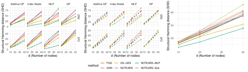
Figure 1: Structure recovery measured by SHD (lower is better) to ground truth. Left: $n=1000$. Middle: $n=200$. Right: Average over all configurations. Rows: random graph model (Erdos-Renyi and scale-free). Columns: different types of SEM. $\mathsf{NOTEARS\mbox{-}MLP}$ performs well on a wide range of settings, while $\mathsf{NOTEARS\mbox{-}Sob}$ shows good accuracy on additive models.

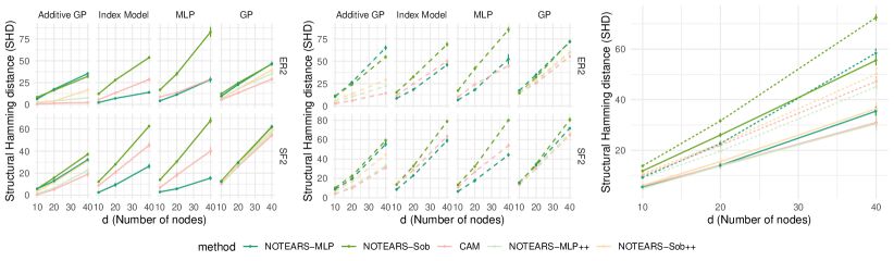
Figure 2: Structure recovery measured by SHD (lower is better) to ground truth. Left: $n=1000$. Middle: $n=200$. Right: Average over all configurations. Rows: random graph model (Erdos-Renyi and scale-free). Columns: different types of SEM. Either $\mathsf{NOTEARS\mbox{-}MLP}$ or $\mathsf{NOTEARS\mbox{-}MLP}\texttt{++}$ (i.e. $\mathsf{NOTEARS\mbox{-}MLP}$ with neighborhood selection and pruning) achieves competitive accuracy compared to $\mathsf{CAM}$.

We study the empirical performance of two instances of the general framework: MLP (4.1) and Sobolev expansions (4.2), denoted by $\mathsf{NOTEARS\mbox{-}MLP}$ and $\mathsf{NOTEARS\mbox{-}Sob}$. For $\mathsf{NOTEARS\mbox{-}MLP}$ we use an MLP with one hidden layer with 10 hidden units and sigmoid activation function. For $\mathsf{NOTEARS\mbox{-}Sob}$ we use Sobolev basis $\varphi_{r}(u)=s_{r}\sin(u/s_{r})$, $s_{r}=2/((2r-1)\pi)$ ($r=1,\dotsc,10$). Complete details on all baselines and simulations, including a discussion of computational complexity and runtimes, can be found in the appendix. Code implementing our method is available at https://github.com/xunzheng/notears.

Baselines

For comparison, the following methods are chosen as baselines: fast greedy equivalence search $(\mathsf{FGS})$ (Ramsey et al., 2017), greedy equivalence search with generalized scores $(\mathsf{GSGES})$ (Huang et al., 2018), DAG-GNN $(\mathsf{GNN})$ (Yu et al., 2019), NOTEARS $(\mathsf{Linear})$ (Zheng et al., 2018) for linear SEM, and causal additive models $(\mathsf{CAM})$ (Bühlmann et al., 2014). To summarize, $\mathsf{FGS}$ and $\mathsf{Linear}$ are specialized at linear models, whereas $\mathsf{GSGES}$, $\mathsf{GNN}$, and $\mathsf{CAM}$ targets general nonlinear dependencies. Comparisons with other score-based methods (KGV score (Bach and Jordan, 2003), Spearman correlation (Sokolova et al., 2014)) and constraint-based methods (PC (Spirtes et al., 2000), MM-MB (Aliferis et al., 2010)) can be found in previous work (Huang et al., 2018), hence are omitted.

Simulation

The ground truth DAG is generated from two random graph models: Erdos-Renyi (ER) and scale-free (SF). We use ER2 to denote an ER graph with $s_{0}=2d$ edges, likewise for SF. Given the ground truth DAG, we simulate the SEM $X_{j}=f_{j}(X_{\operatorname{pa}(j)})+z_{j}$ for all $j\in[d]$ in topological order, and each $z_{j}\sim\mathsf{N}(0,1)$. To evaluate the performance under different data generation mechanisms, we consider four models for the $f_{j}$: 1) Additive models with Gaussian processes (GPs) for each $f_{jk}$, 2) Index models ($M=3$), 3) ANM with MLPs, and 4) ANM with GPs.

Metrics

We evaluate the estimated DAG structure using the following common metrics: false discovery rate (FDR), true positive rate (TPR), false positive rate (FPR), and structural Hamming distance (SHD). Note that both $\mathsf{FGS}$ and $\mathsf{GSGES}$ return a CPDAG that may contain undirected edges, in which case we evaluate them favorably by assuming correct orientation for undirected edges whenever possible, similar to (Zheng et al., 2018).

5.1 Structure learning

In this experiment we examine the structure recovery of different methods by comparing the DAG estimates against the ground truth. We simulate {ER1, ER2, ER4, SF1, SF2, SF4} graphs with $d=\{10,20,40\}$ nodes. For each graph, $n=\{1000,200\}$ data samples are generated. The above process is repeated 10 times and we report the mean and standard deviations of the results. For $\mathsf{NOTEARS\mbox{-}MLP}$ and $\mathsf{NOTEARS\mbox{-}Sob}$, $\lambda=\{0.01,0.03\}$ are used for $n=\{1000,200\}$ respectively.

Figure 1 shows the SHD in various settings; the complete set of results for the remaining metrics are deferred to the supplement. Overall, the proposed $\mathsf{NOTEARS\mbox{-}MLP}$ method attains the best SHD (lower the better) across a wide range of settings, particularly when the data generating mechanism is an MLP or an index model. One can also observe that the performance of $\mathsf{NOTEARS\mbox{-}MLP}$ stays stable for different graph types with varying density and degree distribution, as it does not make explicit assumptions on the topological properties of the graph such as density or degree distribution. Not surprisingly, $\mathsf{NOTEARS\mbox{-}Sob}$ performs well when the underlying SEM is additive GP. On the other hand, when the ground truth is not an additive model, the performance of $\mathsf{NOTEARS\mbox{-}Sob}$ degrades as expected. Finally, we observe that $\mathsf{GSGES}$ outperforms $\mathsf{NOTEARS\mbox{-}MLP}$ and $\mathsf{NOTEARS\mbox{-}Sob}$ on GP, which is a nonparametric setting in which a kernel-based dependency measure can excel, however, we note that the kernel-based approach accompanies an $O(n^{3})$ time complexity, compared to linear dependency on $n$ in $\mathsf{NOTEARS\mbox{-}MLP}$ and $\mathsf{NOTEARS\mbox{-}Sob}$. Also, with by properly tuning the regularization parameter, the performance of $\mathsf{NOTEARS\mbox{-}MLP}$ for each individual setting can be improved considerably, for example in the GP setting. Since such hyperparameter tuning is not the main focus of this paper, we fix a reasonable $\lambda$ for all settings (see Appendix C for more discussion).

With respect to runtime and scalability, we note that the computational complexity of our approach depends on the choice of nonparametric estimator. For example, $\mathsf{NOTEARS\mbox{-}MLP}$ requires $O(nd^{2}m+d^{2}m+d^{3})$ flops per iteration of L-BFGS-B. In terms of runtime, the average runtime of $\mathsf{GSGES}$ on ER2 with $d=40$, $n=1000$ is over 90 minutes, whereas $\mathsf{NOTEARS\mbox{-}MLP}$ takes less than five minutes on average (see Appendix C for more discussion).

Figure 2 shows the SHD compared with $\mathsf{CAM}$. We first observe that $\mathsf{NOTEARS\mbox{-}MLP}$ outperforms $\mathsf{CAM}$ in multiple index models and MLP models, on the other hand, $\mathsf{CAM}$ achieves better accuracy on additive GP and the full GP setting. Recall that the $\mathsf{CAM}$ algorithm involves three steps: 1) Preliminary neighborhood search (PNS), 2) Order search by greedy optimization of the likelihood, and 3) Edge pruning. By comparison, our methods effectively only perform the second step, and can easily be pre- and post-processed with the first (PNS) and third (edge pruning) steps. To further investigate the efficacy of these additional steps, we applied both preliminary neighborhood selection and edge pruning to $\mathsf{NOTEARS\mbox{-}MLP}$ and $\mathsf{NOTEARS\mbox{-}Sob}$ on additive GP and GP settings, denoted as $\mathsf{NOTEARS\mbox{-}MLP}\texttt{++}$ and $\mathsf{NOTEARS\mbox{-}Sob}\texttt{++}$. Noticeably, the output from PNS simply translates to a set of constraints in the form of $\theta_{j}=0$ that can be easily incorporated into the L-BFGS-B algorithm for (13), demonstrating the flexibility of the proposed approach. The performance improves in both cases, matching or improving vs. $\mathsf{CAM}$.

5.2 Sensitivity to number of hidden units

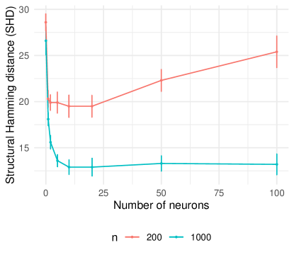
Figure 3: SHD (lower is better) with varying hidden layer size in $\mathsf{NOTEARS\mbox{-}MLP}$.

We also investigated the effect of number of hidden units in the $\mathsf{NOTEARS\mbox{-}MLP}$ estimate. It is well-known that as the size of the hidden layer increases, the functions representable by an MLP become more flexible. On the other hand, larger networks require more samples to estimate the parameters. Indeed, Figure 3 confirms this intuition. We plot the SHD with varying number of hidden units ranging from zero (i.e. linear function) to 100 units, using $n=1000$ and $n=200$ samples generated from the additive GP model on SF2 graph with $d=20$ nodes. One can first observe a sharp phase transition between zero and very few hidden units, which suggests the power of nonlinearity. Moreover, as the number of hidden units increases to 20, the performance for both $n=1000$ and $n=200$ steadily improves, in which case the increased flexibility brings benefit. However, as we further increase the number of hidden units, while SHD for $n=1000$ remains similar, the SHD for $n=200$ deteriorates, hinting at the lack of samples to take advantage of the increased flexibility.

5.3 Real data

Finally, we evaluated $\mathsf{NOTEARS\mbox{-}MLP}$ on a real dataset from Sachs et al. (2005) that is commonly used as a benchmark as it comes with a consensus network that is accepted by the biological community. The dataset consists of $n=7466$ continuous measurements of expression levels of proteins and phospholipids in human immune system cells for $d=11$ cell types. We report an SHD of 16 with 13 edges estimated by $\mathsf{NOTEARS\mbox{-}MLP}$. In comparison, NOTEARS predicts 16 edges with SHD of 22 and $\mathsf{GNN}$ predicts 18 edges that attains SHD of 19. (Due to the large number of samples, we could not run $\mathsf{GSGES}$ on this dataset.) Among the 13 edges predicted by $\mathsf{NOTEARS\mbox{-}MLP}$, 7 edges agree with the consensus network: raf $\to$ mek, mek $\to$ erk, PLCg $\to$ PIP2, PIP3 $\to$ PLCg, PIP3 $\to$ PIP2, PKC $\to$ mek, PKC $\to$ jnk; and 3 edges are predicted but in a reversed direction: raf $\leftarrow$ PKC, akt $\leftarrow$ erk, p38 $\leftarrow$ PKC. Among the true positives, 3 edges are not found by other methods: mek $\to$ erk, PIP3 $\to$ PLCg, PKC $\to$ mek.

6 Discussion

We present a framework for score-based learning of sparse directed acyclic graphical models that subsumes many popular parametric, semiparametric, and nonparametric models as special cases. The key technical device is a notion of nonparametric acyclicity that leverages partial derivatives in the algebraic characterization of DAGs. With a suitable choice of the approximation family, the estimation problem becomes a finite-dimensional differentiable program that can be solved by standard optimization algorithms. The resulting continuous optimization algorithm updates the entire graph (i.e. all edges simultaneously) in each iteration using global information about the current state of the network, as opposed to traditional local search methods that update one edge at a time based on local information. Notably, our approach is generally more efficient and more accurate than existing approaches, despite relying on generic algorithms. This out-of-the-box performance is desirable, especially when noting that future improvements and specializations can be expected to improve the approach substantially.

Acknowledgements

We acknowledge the support of NSF via IIS-1909816, OAC-1934584, ONR via N000141812861, NSF IIS1563887 and DARPA/AFRL FA87501720152. Any opinions, findings and conclusions or recommendations expressed in this material are those of the author(s) and do not necessarily reflect the views of the National Science Foundation, Defense Advanced Research Projects Agency, or Air Force Research Laboratory.

Appendix A Proofs

In this Appendix, we prove Proposition 1. For completeness, note that

$$\mathcal{F}=\{f\ |\ f(u)=\mathsf{MLP}(u;A^{(1)},\ldots,A^{(h)}),$$

$$f\text{ independent of }u_{k}\}$$

and

$$\mathcal{F}_{0}=\{f\ |\ f(u)=\mathsf{MLP}(u;A^{(1)},\ldots,A^{(h)}),$$

$$A^{(1)}_{bk}=0,\forall b=1,\ldots,m_{1}\}.$$

We omit the bias terms in each layer as it does not affect the statement.

Proof of Proposition 1.

We will show that $\mathcal{F}\subseteq\mathcal{F}_{0}$ and $\mathcal{F}_{0}\subseteq\mathcal{F}$.

(1) $\mathcal{F}_{0}\subseteq\mathcal{F}$: for any $f_{0}\in\mathcal{F}_{0}$, we have $f_{0}(u)=\mathsf{MLP}(u;A^{(1)},\ldots,A^{(h)})$, where $A^{(1)}_{bk}=0$ for all $b=1,\dotsc,m_{1}$. Hence the linear function $A^{(1)}u$ is independent of $u_{k}$. Therefore,

$$f_{0}(u) =\mathsf{MLP}(u;A^{(1)},\ldots,A^{(h)})$$

$$=\sigma(A^{(h)}\sigma(\cdots A^{(2)}\sigma(A^{(1)}u)))$$

is also independent of $u_{k}$, which means $f_{0}\in\mathcal{F}$.

(2) $\mathcal{F}\subseteq\mathcal{F}_{0}$: for any $f\in\mathcal{F}$, we have $f(u)=\mathsf{MLP}(u;A^{(1)},\ldots,A^{(h)})$ and $f$ is independent of $u_{k}$. We will show that $f\in\mathcal{F}_{0}$ by constructing a matrix $\tilde{A}^{(1)}$, such that

$$f(u)=\mathsf{MLP}(u;\tilde{A}^{(1)},{A}^{(2)},\ldots,A^{(h)})$$ (14)

and $\tilde{A}_{bk}^{(1)}=0$ for all $b=1,\dotsc,m_{1}$.

Let $\tilde{u}$ be the vector such that $\tilde{u}_{k}=0$ and $\tilde{u}_{k^{\prime}}=u_{k}$ for all $k^{\prime}\neq k$. Since $\tilde{u}$ and $u$ differ only on the $k$th dimension, and $f$ is independent of $u_{k}$, we have

$$f(u)=f(\tilde{u})=\mathsf{MLP}(\tilde{u};A^{(1)},\ldots,A^{(h)}).$$ (15)

Now define $\tilde{A}^{(1)}$ be the matrix such that $\tilde{A}_{bk}^{(1)}=0$ and $\tilde{A}_{bk^{\prime}}^{(1)}={A}_{bk}^{(1)}$ for all $k^{\prime}\neq k$. Then we have the following observation: for each entry $s\in\{1,\dotsc,m_{1}\}$,

$$(\tilde{A}^{(1)}u)_{s} =\sum_{k^{\prime}=1}^{d}\tilde{A}_{sk^{\prime}}u_{k^{\prime}}=\sum_{k^{\prime}\neq k}A_{sk^{\prime}}u_{k^{\prime}}$$

$$=\sum_{k^{\prime}=1}^{d}A_{sk^{\prime}}\tilde{u}_{k^{\prime}}=({A}^{(1)}\tilde{u})_{s}.$$

Hence,

$$\tilde{A}^{(1)}u={A}^{(1)}\tilde{u}.$$ (16)

Therefore, by (15)

$$f(u) =f(\tilde{u})$$

$$=\mathsf{MLP}(\tilde{u};A^{(1)},\ldots,A^{(h)})$$

$$=\sigma(A^{(h)}\sigma(\cdots A^{(2)}\sigma(A^{(1)}\tilde{u})))$$

$$=\sigma(A^{(h)}\sigma(\cdots A^{(2)}\sigma(\tilde{A}^{(1)}u)))$$

$$=\mathsf{MLP}(u;\tilde{A}^{(1)},A^{(2)},\ldots,A^{(h)})$$

By definition of $\mathcal{F}_{0}$, we know that $\mathsf{MLP}(u;\tilde{A}^{(1)},A^{(2)},\ldots,A^{(h)})\in\mathcal{F}_{0}$. Thus, $f\in\mathcal{F}_{0}$ and we have completed the proof. ∎

Appendix B Experiment details

Baselines

We consider the following baselines.

• Fast greedy equivalence search $(\mathsf{FGS})$ (Ramsey et al., 2017) is based on greedy search and assumes linear dependency between variables.

• Greedy equivalence search with generalized scores $(\mathsf{GSGES})$ (Huang et al., 2018) is also based on greedy search, but uses generalized scores without assuming a particular model class.

• DAG-GNN $(\mathsf{GNN})$ (Yu et al., 2019) learns a (noisy) nonlinear transformation of a linear SEM using neural networks.

• NOTEARS $(\mathsf{Linear})$ (Zheng et al., 2018) learns a linear SEM using continuous optimization.

• Causal additive model $(\mathsf{CAM})$ (Bühlmann et al., 2014) learns an additive SEM by leveraging efficient nonparametric regression techniques and greedy search over edges.

For all experiments, default parameter settings are used, except for $\mathsf{CAM}$ where both preliminary neighborhood selection and pruning are applied.

Simulation

Given the graph $\mathsf{G}$, we simulate the SEM $X_{j}=f_{j}(X_{\operatorname{pa}(j)})+z_{j}$ for all $j\in[d]$ in the topological order induced by $\mathsf{G}$. We consider the following instances of $f_{j}$:

• Additive GP: $f_{j}(X_{\operatorname{pa}(j)})=\sum_{k\in\operatorname{pa}(j)}f_{jk}(X_{k})$, where each $f_{jk}$ is a draw from Gaussian process with RBF kernel with length-scale one.

• Index model: $f_{j}(X_{\operatorname{pa}(j)})=\sum_{m=1}^{3}h_{m}(\sum_{k\in\operatorname{pa}(j)}\theta_{jmk}X_{k})$, where $h_{1}=\tanh$, $h_{2}=\cos$, $h_{3}=\sin$, and each $\theta_{jmk}$ is drawn uniformly from range $[-2,-0.5]\cup[0.5,2]$.

• MLP: $f_{j}$ is a randomly initialized MLP with one hidden layer of size 100 and sigmoid activation.

• GP: $f_{j}$ is a draw from Gaussian process with RBF kernel with length-scale one.

In all settings, $z_{j}$ is i.i.d. standard Gaussian noise.

Appendix C Additional results

Full comparison

We show {SHD, FDR, TPR, FPR} results on all {ER1, ER2, ER4, SF1, SF2, SF4} graphs in Figure 4, 5, 6, 7 respectively. Similarly, see Figure 8, 9, 10, 11 for full comparison with $\mathsf{CAM}$. As in Figure 1, each row is a random graph model, each column is a type of SEM. Overall $\mathsf{NOTEARS\mbox{-}MLP}$ has low FDR/FPR and high TPR, and same for $\mathsf{NOTEARS\mbox{-}Sob}$ on additive GP. Also observe that in most settings $\mathsf{GNN}$ has low FDR as well as low TPR, which is a consequence of only predicting a small number of edges.

Complexity and runtime

	$\mathsf{NOTEARS\mbox{-}MLP}$	$\mathsf{NOTEARS\mbox{-}Sob}$	$\mathsf{FGS}$	$\mathsf{Linear}$	$\mathsf{GNN}$	$\mathsf{GSGES}$
$d=20$	92.12 $\pm$ 22.51	62.90 $\pm$ 16.83	0.55 $\pm$ 0.43	10.95 $\pm$ 4.52	498.32 $\pm$ 43.72	1547.42 $\pm$ 109.83
$d=40$	282.64 $\pm$ 67.46	321.88 $\pm$ 57.33	0.59 $\pm$ 0.17	43.15 $\pm$ 12.43	706.35 $\pm$ 64.49	6379.98 $\pm$ 359.67

Table 1: Runtime (in seconds) of various algorithms on ER2 graph with $n=1000$ samples.

Recall that numerical evaluation of matrix exponential involves solving linear systems, hence the time complexity is typically $O(d^{3})$ for a dense $d\times d$ matrix. Taking $\mathsf{NOTEARS\mbox{-}MLP}$ with one hidden layer of $m$ units as an example, it takes $O(nd^{2}m+d^{2}m+d^{3})$ time to evaluate the objective and the gradient. If $m/d=O(1)$, this is comparable to the linear case $O(nd^{2}+d^{3})$, except for the inevitable extra cost from using a nonlinear function. This highlights the benefit of Proposition 1: the acyclicity constraint almost comes for free. Furthermore, we used a quasi-Newton method to reduce the number of calls to evaluate the gradient, which involves computing the matrix exponential. Table 1 contains runtime comparison of different algorithms on ER2 graph with $n=1000$ samples. Recall that the kernel-based approach of $\mathsf{GSGES}$ comes with a $O(n^{3})$ computational complexity, whereas $\mathsf{NOTEARS\mbox{-}MLP}$ and $\mathsf{NOTEARS\mbox{-}Sob}$ has $O(n)$ dependency on $n$. This can be confirmed from the table, which shows $\mathsf{GSGES}$ has a significantly longer runtime.

Comments on hyperparameter tuning

The experiments presented in this paper were conducted under a fixed (and therefore suboptimal) value of $\lambda$ and weight threshold across all graph types, sparsity levels, and SEM types, despite the fact that each configuration may prefer different regularization strengths. Indeed, we observe substantially improved performance by choosing different values of hyperparameters in some settings. As our focus is not on attaining the best possible accuracy in all settings by carefully tuning the hyperparameters, we omit these results in the main text and only include here as a supplement. For instance, for ER4 graph with $d=40$ variables and $n=200$ samples, when the SEM is additive GP and MLP, setting $\lambda=0.03$ and threshold = 0.5 gives results summarized in Table 2.

SEM	Method	SHD	FDR	TPR	FPR	Predicted #
Additive-GP	$\mathsf{NOTEARS\mbox{-}MLP}$	124.3 $\pm$ 6.65	0.30 $\pm$ 0.07	0.35 $\pm$ 0.04	0.04 $\pm$ 0.01	81.70 $\pm$ 10.49
	$\mathsf{GSGES}$	121.3 $\pm$ 5.02	0.36 $\pm$ 0.05	0.28 $\pm$ 0.03	0.04 $\pm$ 0.00	69.30 $\pm$ 5.01
MLP	$\mathsf{NOTEARS\mbox{-}MLP}$	88.40 $\pm$ 11.29	0.18 $\pm$ 0.08	0.57 $\pm$ 0.06	0.03 $\pm$ 0.02	111.70 $\pm$ 15.97
	$\mathsf{GSGES}$	121.60 $\pm$ 11.95	0.33 $\pm$ 0.09	0.33 $\pm$ 0.06	0.04 $\pm$ 0.01	77.10 $\pm$ 7.13

Table 2: ER4, $d=40$, $n=200$ with $\lambda=0.03$ and threshold = 0.5.

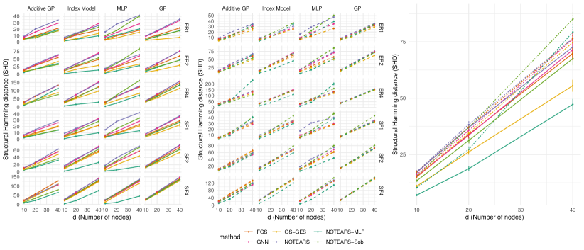
Figure 4: Structure recovery measured by SHD (lower is better) to ground truth.

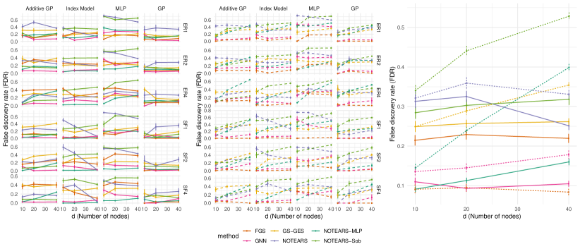
Figure 5: Structure recovery measured by FDR (lower is better) to ground truth.

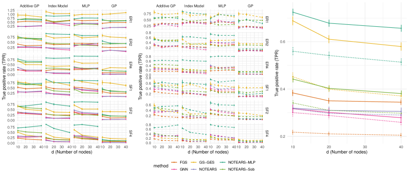
Figure 6: Structure recovery measured by TPR (higher is better) to ground truth.

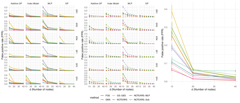
Figure 7: Structure recovery measured by FPR (lower is better) to ground truth.

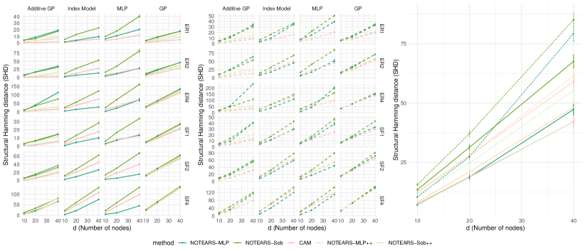
Figure 8: Structure recovery measured by SHD (lower is better) to ground truth, compared with $\mathsf{CAM}$.

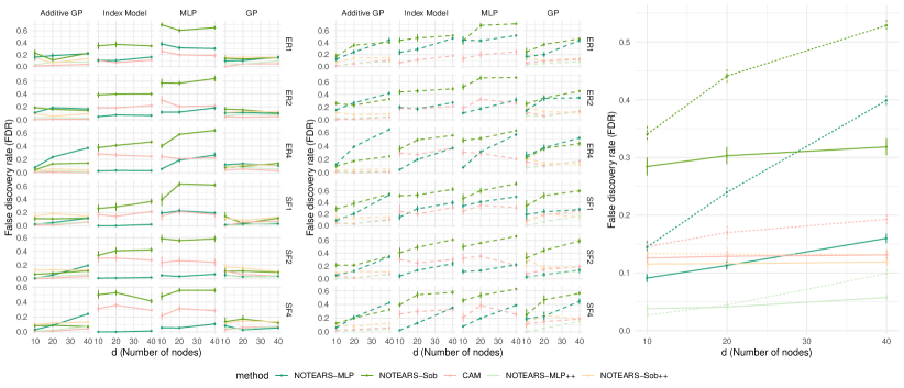
Figure 9: Structure recovery measured by FDR (lower is better) to ground truth, compared with $\mathsf{CAM}$.

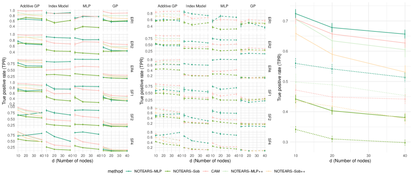
Figure 10: Structure recovery measured by TPR (higher is better) to ground truth, compared with $\mathsf{CAM}$.

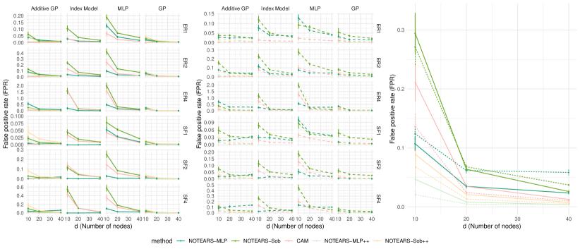
Figure 11: Structure recovery measured by FPR (lower is better) to ground truth, compared with $\mathsf{CAM}$.

References

- Abid et al. (2019) A. Abid, M. F. Balin, and J. Zou. Concrete Autoencoders for Differentiable Feature Selection and Reconstruction. In International Conference on Machine Learning, 2019.
- Aliferis et al. (2010) C. F. Aliferis, A. Statnikov, I. Tsamardinos, S. Mani, and X. D. Koutsoukos. Local causal and markov blanket induction for causal discovery and feature selection for classification part i: Algorithms and empirical evaluation. Journal of Machine Learning Research, 11(Jan):171–234, 2010.
- Alquier and Biau (2013) P. Alquier and G. Biau. Sparse single-index model. Journal of Machine Learning Research, 14(Jan):243–280, 2013.
- Aragam and Zhou (2015) B. Aragam and Q. Zhou. Concave penalized estimation of sparse Gaussian Bayesian networks. Journal of Machine Learning Research, 16:2273–2328, 2015.
- Bach and Jordan (2003) F. R. Bach and M. I. Jordan. Learning graphical models with mercer kernels. In Advances in Neural Information Processing Systems, pages 1033–1040, 2003.
- Banerjee et al. (2008) O. Banerjee, L. El Ghaoui, and A. d’Aspremont. Model selection through sparse maximum likelihood estimation for multivariate Gaussian or binary data. Journal of Machine Learning Research, 9:485–516, 2008.
- Bertin et al. (2008) K. Bertin, G. Lecué, et al. Selection of variables and dimension reduction in high-dimensional non-parametric regression. Electronic Journal of Statistics, 2:1224–1241, 2008.
- Blöbaum et al. (2018) P. Blöbaum, D. Janzing, T. Washio, S. Shimizu, and B. Schölkopf. Cause-Effect Inference by Comparing Regression Errors. In International Conference on Artificial Intelligence and Statistics, 2018.
- Bühlmann et al. (2014) P. Bühlmann, J. Peters, and J. Ernest. CAM: Causal additive models, high-dimensional order search and penalized regression. Annals of Statistics, 2014.
- Byrd et al. (1995) R. H. Byrd, P. Lu, J. Nocedal, and C. Zhu. A limited memory algorithm for bound constrained optimization. SIAM Journal on Scientific Computing, 1995.
- Chen et al. (2018) W. Chen, M. Drton, and Y. S. Wang. On causal discovery with equal variance assumption. 07 2018.
- Diaconis and Shahshahani (1984) P. Diaconis and M. Shahshahani. On nonlinear functions of linear combinations. SIAM Journal on Scientific and Statistical Computing, 5(1):175–191, 1984.
- Efromovich (2008) S. Efromovich. Nonparametric curve estimation: methods, theory, and applications. Springer Science & Business Media, 2008.
- Ernest et al. (2016) J. Ernest, D. Rothenhäusler, and P. Bühlmann. Causal inference in partially linear structural equation models: identifiability and estimation. arXiv preprint arXiv:1607.05980, 2016.
- Feng and Simon (2017) J. Feng and N. Simon. Sparse-Input Neural Networks for High-dimensional Nonparametric Regression and Classification. arXiv preprint arXiv:1711.07592, 2017.
- Fukumizu et al. (2008) K. Fukumizu, A. Gretton, X. Sun, and B. Schölkopf. Kernel measures of conditional dependence. In Advances in neural information processing systems, pages 489–496, 2008.
- Ghoshal and Honorio (2017) A. Ghoshal and J. Honorio. Learning identifiable gaussian bayesian networks in polynomial time and sample complexity. In Advances in Neural Information Processing Systems, 2017.
- Goudet et al. (2018) O. Goudet, D. Kalainathan, P. Caillou, I. Guyon, D. Lopez-Paz, and M. Sebag. Learning Functional Causal Models with Generative Neural Networks. In Explainable and Interpretable Models in Computer Vision and Machine Learning. Springer, 2018.
- Gregorová et al. (2018) M. Gregorová, A. Kalousis, and S. Marchand-Maillet. Structured nonlinear variable selection. In Uncertainty in Artificial Intelligence, 2018.
- Gretton et al. (2005) A. Gretton, O. Bousquet, A. Smola, and B. Schölkopf. Measuring statistical dependence with hilbert-schmidt norms. In International conference on algorithmic learning theory, pages 63–77. Springer, 2005.
- Gu et al. (2018) J. Gu, F. Fu, and Q. Zhou. Penalized estimation of directed acyclic graphs from discrete data. Statistics and Computing, DOI: 10.1007/s11222-018-9801-y, 2018.
- Hall (1987) P. Hall. Cross-validation and the smoothing of orthogonal series density estimators. Journal of multivariate analysis, 21(2):189–206, 1987.
- Hastie and Tibshirani (1987) T. Hastie and R. Tibshirani. Generalized additive models: some applications. Journal of the American Statistical Association, 82(398):371–386, 1987.
- Heckerman et al. (1992) D. Heckerman, E. Horvitz, and B. Nathwani. Toward normative expert systems: Part i, the pathfinder project. knowledge systems laboratory, medical computer science, 1992.
- Hoyer et al. (2009) P. O. Hoyer, D. Janzing, J. M. Mooij, J. Peters, and B. Schölkopf. Nonlinear causal discovery with additive noise models. In Advances in neural information processing systems, pages 689–696, 2009.
- Hsieh et al. (2013) C.-J. Hsieh, M. A. Sustik, I. S. Dhillon, P. K. Ravikumar, and R. Poldrack. Big & quic: Sparse inverse covariance estimation for a million variables. In Advances in Neural Information Processing Systems, pages 3165–3173, 2013.
- Huang et al. (2018) B. Huang, K. Zhang, Y. Lin, B. Schölkopf, and C. Glymour. Generalized score functions for causal discovery. In KDD, 2018.
- Kagan et al. (1973) A. M. Kagan, C. R. Rao, and Y. V. Linnik. Characterization problems in mathematical statistics. Wiley, 1973.
- Kalainathan et al. (2018) D. Kalainathan, O. Goudet, I. Guyon, D. Lopez-Paz, and M. Sebag. SAM: Structural Agnostic Model, Causal Discovery and Penalized Adversarial Learning. arXiv preprint arXiv:1803.04929, 2018.
- Kusner et al. (2017) M. J. Kusner, J. Loftus, C. Russell, and R. Silva. Counterfactual fairness. In Advances in Neural Information Processing Systems, pages 4066–4076, 2017.
- Lachapelle et al. (2019) S. Lachapelle, P. Brouillard, T. Deleu, and S. Lacoste-Julien. Gradient-Based Neural DAG Learning. arXiv preprint arXiv:1906.02226, 2019.
- Lafferty et al. (2008) J. Lafferty, L. Wasserman, et al. Rodeo: sparse, greedy nonparametric regression. The Annals of Statistics, 36(1):28–63, 2008.
- Lee et al. (2016) A. B. Lee, R. Izbicki, et al. A spectral series approach to high-dimensional nonparametric regression. Electronic Journal of Statistics, 10(1):423–463, 2016.
- Liu et al. (2009) H. Liu, J. Lafferty, and L. Wasserman. The nonparanormal: Semiparametric estimation of high dimensional undirected graphs. Journal of Machine Learning Research, 2009.
- Loh and Bühlmann (2014) P.-L. Loh and P. Bühlmann. High-dimensional learning of linear causal networks via inverse covariance estimation. Journal of Machine Learning Research, 15:3065–3105, 2014.
- Miller et al. (2010) H. Miller, P. Hall, et al. Local polynomial regression and variable selection. In Borrowing Strength: Theory Powering Applications–A Festschrift for Lawrence D. Brown, pages 216–233. Institute of Mathematical Statistics, 2010.
- Monti et al. (2019) R. P. Monti, K. Zhang, and A. Hyvärinen. Causal Discovery with General Non-Linear Relationships Using Non-Linear ICA. arXiv preprint arXiv:1904.09096, 2019.
- Mooij et al. (2016) J. M. Mooij, J. Peters, D. Janzing, J. Zscheischler, and B. Schölkopf. Distinguishing Cause from Effect Using Observational Data: Methods and Benchmarks. Journal of Machine Learning Research, 2016.
- Park (2018) G. Park. Learning generalized hypergeometric distribution (ghd) dag models. arXiv preprint arXiv:1805.02848, 2018.
- Park and Park (2019) G. Park and S. Park. High-dimensional poisson structural equation model learning via -regularized regression. Journal of Machine Learning Research, 20(95):1–41, 2019. URL http://jmlr.org/papers/v20/18-819.html.
- Park and Raskutti (2017) G. Park and G. Raskutti. Learning quadratic variance function (qvf) dag models via overdispersion scoring (ods). 04 2017.
- Peters and Bühlmann (2013) J. Peters and P. Bühlmann. Identifiability of Gaussian structural equation models with equal error variances. Biometrika, 101(1):219–228, 2013.
- Peters et al. (2014) J. Peters, J. Mooij, D. Janzing, and B. Schölkopf. Causal Discovery with Continuous Additive Noise Models. Journal of Machine Learning Research, 2014.
- Ramsey et al. (2017) J. Ramsey, M. Glymour, R. Sanchez-Romero, and C. Glymour. A million variables and more: the Fast Greedy Equivalence Search algorithm for learning high-dimensional graphical causal models, with an application to functional magnetic resonance images. International Journal of Data Science and Analytics, 2017.
- Ravikumar et al. (2009) P. Ravikumar, J. Lafferty, H. Liu, and L. Wasserman. Sparse additive models. Journal of the Royal Statistical Society: Series B (Statistical Methodology), 71(5):1009–1030, 2009.
- Rosasco et al. (2013) L. Rosasco, S. Villa, S. Mosci, M. Santoro, and A. Verri. Nonparametric sparsity and regularization. Journal of Machine Learning Research, 2013.
- Sachs et al. (2005) K. Sachs, O. Perez, D. Pe’er, D. A. Lauffenburger, and G. P. Nolan. Causal Protein-Signaling Networks Derived from Multiparameter Single-Cell Data. Science, 2005.
- Sanford and Moosa (2012) A. D. Sanford and I. A. Moosa. A bayesian network structure for operational risk modelling in structured finance operations. Journal of the Operational Research Society, 63(4):431–444, 2012.
- Schwartz (1967) S. C. Schwartz. Estimation of probability density by an orthogonal series. The Annals of Mathematical Statistics, pages 1261–1265, 1967.
- Sgouritsa et al. (2015) E. Sgouritsa, D. Janzing, P. Hennig, and B. Schölkopf. Inference of cause and effect with unsupervised inverse regression. In Artificial intelligence and statistics, pages 847–855, 2015.
- Shimizu et al. (2006) S. Shimizu, P. O. Hoyer, A. Hyvärinen, and A. Kerminen. A linear non-Gaussian acyclic model for causal discovery. Journal of Machine Learning Research, 7:2003–2030, 2006.
- Sokolova et al. (2014) E. Sokolova, P. Groot, T. Claassen, and T. Heskes. Causal discovery from databases with discrete and continuous variables. In European Workshop on Probabilistic Graphical Models, pages 442–457. Springer, 2014.
- Spirtes et al. (2000) P. Spirtes, C. Glymour, and R. Scheines. Causation, prediction, and search, volume 81. The MIT Press, 2000.
- Suggala et al. (2017) A. Suggala, M. Kolar, and P. K. Ravikumar. The expxorcist: Nonparametric graphical models via conditional exponential densities. In Advances in Neural Information Processing Systems 30, pages 4446–4456. 2017.
- Tagasovska et al. (2018) N. Tagasovska, T. Vatter, and V. Chavez-Demoulin. Nonparametric quantile-based causal discovery. arXiv preprint arXiv:1801.10579, 2018.
- Tsybakov (2009) A. Tsybakov. Introduction to nonparametric estimation. Springer Series in Statistics, New York, page 214, 2009. cited By 1.
- Voorman et al. (2014) A. Voorman, A. Shojaie, and D. Witten. Graph estimation with joint additive models. Biometrika, 2014.
- Wahba (1981) G. Wahba. Data-based optimal smoothing of orthogonal series density estimates. The annals of statistics, pages 146–156, 1981.
- Yang et al. (2015) E. Yang, P. Ravikumar, G. I. Allen, and Z. Liu. Graphical models via univariate exponential family distributions. Journal of Machine Learning Research, 16:3813–3847, 2015.
- Ye and Sun (2018) M. Ye and Y. Sun. Variable Selection via Penalized Neural Network: a Drop-Out-One Loss Approach. In International Conference on Machine Learning, 2018.
- Yu et al. (2019) Y. Yu, J. Chen, T. Gao, and M. Yu. Dag-gnn: Dag structure learning with graph neural networks. arXiv preprint arXiv:1904.10098, 2019.
- Yuan (2011) M. Yuan. On the identifiability of additive index models. Statistica Sinica, 21(4):1901, 2011.
- Zhang and Hyvärinen (2009) K. Zhang and A. Hyvärinen. On the identifiability of the post-nonlinear causal model. In Proceedings of the twenty-fifth conference on uncertainty in artificial intelligence, pages 647–655. AUAI Press, 2009.
- Zhang and Hyvärinen (2009) K. Zhang and A. Hyvärinen. On the Identifiability of the Post-Nonlinear Causal Model. In Uncertainty in Artificial Intelligence, 2009.
- Zhang et al. (2012) K. Zhang, J. Peters, D. Janzing, and B. Schölkopf. Kernel-based conditional independence test and application in causal discovery. arXiv preprint arXiv:1202.3775, 2012.
- Zhang et al. (2016) K. Zhang, Z. Wang, J. Zhang, and B. Schölkopf. On estimation of functional causal models: general results and application to the post-nonlinear causal model. ACM Transactions on Intelligent Systems and Technology (TIST), 7(2):13, 2016.
- Zheng et al. (2018) X. Zheng, B. Aragam, P. Ravikumar, and E. P. Xing. DAGs with NO TEARS: Continuous Optimization for Structure Learning. In Advances in Neural Information Processing Systems, 2018.