Causal screening in dynamical systems

Abstract

Many classical algorithms output graphical representations of causal structures by testing conditional independence among a set of random variables. In dynamical systems, local independence can be used analogously as a testable implication of the underlying data-generating process. We suggest some inexpensive methods for causal screening which provide output with a sound causal interpretation under the assumption of ancestral faithfulness. The popular model class of linear Hawkes processes is used to provide an example of a dynamical causal model. We argue that for sparse causal graphs the output will often be close to complete. We give examples of this framework and apply it to a challenging biological system.

1 INTRODUCTION

Constraint-based causal learning is computationally and statistically challenging. There is a large literature on learning structures that are represented by directed acyclic graphs (DAGs) or marginalizations thereof (see Maathuis et al. (2019) for references). The fast causal inference algorithm (FCI, Spirtes et al., 2000) provides in a certain sense maximally informative output (Zhang, 2008), but at the cost of using a large number of conditional independence tests (Colombo et al., 2012). To reduce the computational cost, other methods provide output which has a sound causal interpretation, but may be less informative. Among these are the anytime FCI (Spirtes, 2001) and RFCI (Colombo et al., 2012). A recent algorithm, ancestral causal inference (ACI, Magliacane et al., 2016), aims to learn only the directed part of the underlying graphical structure which allows for a sound causal interpretation even though some information is lost.

In this paper, we describe some simple methods for learning causal structure in dynamical systems represented by stochastic processes. Many authors have described frameworks and algorithms for learning structure in systems of time series, ordinary differential equations, stochastic differential equations, and point processes. However, most of these methods do not have a clear causal interpretation when the observed processes are part of a larger system and most of the current literature is either non-causal in nature, or requires that there are no unobserved processes.

Analogously to testing conditional independence when learning DAGs, one can use tests of local independence in the case of dynamical systems. Eichler (2013), Meek (2014), and Mogensen et al. (2018) propose algorithms for learning graphs that represent local independence structures. We show empirically that we can recover features of their graphical learning target using considerably fewer tests of local independence. First, we suggest a learning target which is easier to learn, though still conveys useful causal information, analogously to ACI (Magliacane et al., 2016). Second, the proposed algorithm is only guaranteed to provide a supergraph of the learning target and this also reduces the number of local independence tests drastically. A central point is that our proposed methods retain a causal interpretation in the sense that absent edges in the output correspond to implausible causal connections.

Meek (2014) suggests learning a directed graph to represent a causal dynamical system and gives a learning algorithm which we will describe as a simple screening algorithm (Section 4.2). We show that this algorithm can be given a sound interpretation under a weaker faithfulness assumption than that of Meek (2014). We also provide a simple interpretation of the output of this algorithm and we show that similar screening algorithms can give comparable results using considerably fewer tests of local independence.

All proofs are provided in the supplementary material.

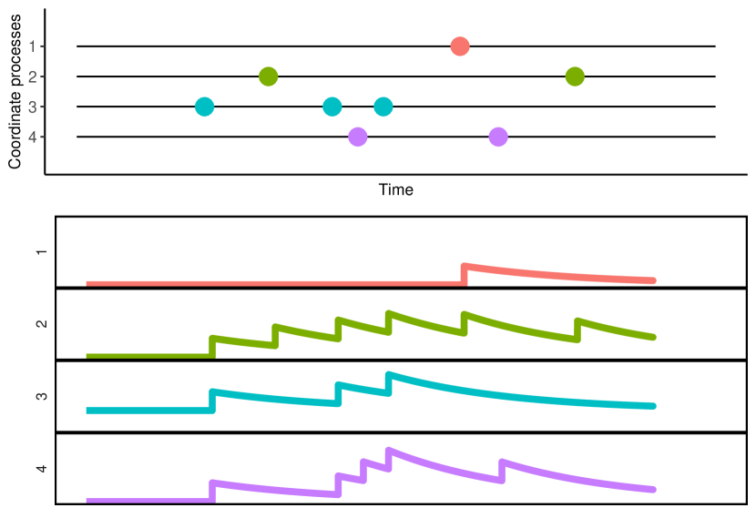
(a) Top: Example data from a four-dimensional Hawkes process. Bottom: The corresponding intensities. The time axis is aligned between the two plots.

(b) Left: The causal graph (see Section 2.1) of a four-dimensional Hawkes process. Right: Learning output of standard approach (see Section 2) when 3 is unobserved. When 3 is unobserved, 2 is predictive of 4 and vice versa (heuristically, more events in process 2 indicate more events in 3 which in turn indicates more events in 4). However, they are not causally connected and using local independence one can learn that 2 is not a parent of 4. This is important to predict what would happen under interventions in the system as the right-hand graph indicates that an intervention on 2 would change the distribution of 4 even though this is not the case as $g^{\alpha 2}=0$ for $\alpha\in\{1,3,4\}$.

Figure 1: Subfigure 1(a) shows data generated from the system in 1(b) (left). Until the first event all intensities are constant (equal to $\mu_{\alpha}$ for the $\alpha$-process). The first event occurs in process 3. We see that $g^{23}$, $g^{33}$, and $g^{43}$ are different from zero as encoded by the graph in 1(b) (left). Therefore the event makes the intensity processes of 2, 3, and 4 jump, making new events in these processes more likely in the immediate future (1(a), bottom).

2 HAWKES PROCESSES

Local independence can be defined in a wide range of discrete-time and continous-time dynamical models (e.g., point processes (Didelez, 2000), time series (Eichler, 2012), and diffusions (Mogensen et al., 2018). See also Commenges and Gégout-Petit (2009)), and the algorithmic results we present apply to all these classes of models. However, the causal interpretation will differ between these model classes, and we will use the linear Hawkes processes to exemplify the framework. Laub et al. (2015) give an accessible introduction to this continuous-time model class and Liniger (2009), Bacry et al. (2015), and Daley and Vere-Jones (2003) provide more background. Hawkes processes have also been studied in the machine learning community in recent years (Zhou et al., 2013a, b; Luo et al., 2015; Xu et al., 2016; Etesami et al., 2016; Achab et al., 2017; Tan et al., 2018; Xu et al., 2018; Trouleau et al., 2019). It is important to note that these papers all consider the case of full observation, i.e., every coordinate process is observed. In causal systems that are not fully observed that assumption may lead to false conclusions (see Figure 1(b)). Our work addresses the learning problem without the assumption of full observation, hence there can be unknown and unobserved confounding processes.

On a filtered probability space, $(\Omega,\mathcal{F},(\mathcal{F}_{t}),\text{P})$, we consider an $n$-dimensional multivariate point process, $X=(X^{1},\ldots,X^{n})$. $\mathcal{F}_{t}$ is a filtration, i.e., a nondecreasing family of $\sigma$-algebras, and it represents the information which is available at a specific time point. Each coordinate process $X^{\alpha}$ is described by a sequence of positive, stochastic event times $T_{1}^{\alpha},T_{2}^{\alpha},\ldots$ such that $T_{j}^{\alpha}>T_{i}^{\alpha}$ almost surely for $j>i$. We let $V=\{1,\ldots,n\}$. This can also be formulated in terms of a counting process, $N$, such that $N_{s}^{\alpha}=\sum_{i}\mathds{1}_{(T_{i}\leq s)}$, $\alpha\in V$. There exists so-called intensity processes, $\lambda=(\lambda^{1},\ldots,\lambda^{n})$, such that

$$\lambda_{t}^{\alpha}=\lim_{h\rightarrow 0}\frac{1}{h}\text{P}(N_{t+h}^{\alpha}-N_{t}^{\alpha}=1\mid\mathcal{F}_{t})$$

and the intensity at time $t$ can therefore be thought of as describing the probability of a jump in the immediate future after time $t$ conditionally on the history until time $t$ as captured by the $\mathcal{F}_{t}$-filtration. In a linear Hawkes model, the intensity of the $\alpha$-process, $\alpha\in V$, is of the simple form

$$\lambda_{t}^{\alpha} =\mu_{\alpha}+\sum_{\gamma\in V}\int_{0}^{t}g^{\alpha\gamma}(t-s)\ \mathrm{d}N_{s}^{\gamma}$$

$$=\mu_{\alpha}+\sum_{\gamma\in V}\sum_{i:T_{i}^{\gamma}<t}g^{\alpha\gamma}(t-T_{i}^{\gamma})$$

where $\mu_{\alpha}\geq 0$ and the function $g^{\alpha\gamma}:\mathbb{R}_{+}\rightarrow\mathbb{R}$ is nonnegative for all $\alpha,\gamma\in V$. From the above formula, we see that if $g^{\beta\alpha}=0$, then the $\alpha$-process does not enter directly into the intensity of the $\beta$-process and we will formalize this observation in subsequent sections. The intensity processes determine how the Hawkes process evolves and if $g^{\beta\alpha}=0$ then the $\alpha$-process does not directly influence the evolution of the $\beta$-process (it may of course have an indirect influence which is mediated by other processes). Figure 1(a) provides an example of data from a linear Hawkes process and an illustration of its intensity processes.

Figure 2: Left: A causal graph on nodes $V=\{\alpha,\beta,\gamma,\delta,\epsilon,\phi\}$. Right: The corresponding parent graph on nodes $O=\{\alpha,\delta,\epsilon\}$. Note that causal graphs and parent graphs may contain cycles. The parent graph does not contain information on the confounder process $\phi$ as it only encodes ‘causal ancestors’. One can also marginalize the causal graph to obtain a directed mixed graph from which one can read off the parent graph (see the supplementary material).

2.1 A DYNAMICAL CAUSAL MODEL

We will in this section define what we mean by a dynamical causal model in the case of a linear Hawkes process and also define a graph $(V,E)$ which represents the causal structure of the model. The node set $V$ is the index set of the coordinate processes of the multivariate Hawkes process, thus identifying each node with a coordinate process. If we first consider the case where $X=(X_{1},\ldots,X_{n})$ is a multivariate random variable, it is common to define a causal model in terms of a DAG, $\mathcal{D}$, and a structural causal model (Pearl, 2009; Peters et al., 2017) by assuming that there exists functions $f_{i}$ and error terms $\epsilon_{i}$ such that

$$X_{i}=f_{i}(X_{\text{pa}_{\mathcal{D}}(X_{i})},\epsilon_{i})$$

for $i=1,\ldots,n$. The causal assumption amounts to assuming that the functional relations are stable under interventions. This idea can be transferred to dynamical systems (see also Røysland (2012); Mogensen et al. (2018)). In the case of a linear Hawkes process as described above, we can consider intervening on the $\alpha$-process and force events to occur at the deterministic times $t_{1},\ldots,t_{k}$, and at these times only. In this case, the causal assumption amounts to assuming that the distribution of the intervened system is governed by the intensities

$$\lambda_{t}^{\beta}=\mu_{\beta} +\int_{0}^{t}g^{\beta\alpha}(t-s)\ \mathrm{d}\bar{N}_{s}^{\alpha}$$

$$+\sum_{\gamma\in V\setminus\{\alpha\}}\int_{0}^{t}g^{\beta\gamma}(t-s)\ \mathrm{d}N_{s}^{\gamma}$$

for all $\beta\in V\setminus\{\alpha\}$ and where $\bar{N}_{t}^{\alpha}=\sum_{i=1}^{k}\mathds{1}_{(t_{i}\leq t)}$. We will not go into a discussion of the existence of these interventional stochastic processes. The above is a hard intervention in the sense that the $\alpha$-process is fixed to be a deterministic function of time. Note that one could easily imagine other types of interventions such as soft interventions where the intervention process, $\alpha$, is not deterministic. One can also extend this to interventions on more than one process. It holds that $N_{t+h}^{\beta}-N_{t}^{\beta}\sim\operatorname{Pois}(\lambda_{t}^{\beta}\cdot h)$ in the limit $h\rightarrow 0$, and we can think of this as a simulation scheme in which we generate the points in one small interval in accordance to some distribution depending on the history of the process. As such the intensity describes a structural causal model at infinitesimal time steps and the $g^{\alpha\beta}$-functions are in a causal model stable under interventions in the sense that they also describe how the intervention process $\bar{N}^{\alpha}$ enters into the intensity of the other processes.

We use the set of functions $\{g^{\beta\alpha}\}_{\alpha,\beta\in V}$ to define the causal graph of the Hawkes process. A graph is a pair $(V,E)$ where $V$ is a set of nodes and $E$ is a set of edges between these nodes. We assume that we observe the Hawkes process in the time interval $J=[0,T]$, $T\in\mathbb{R}$. The causal graph has node set $V$ (the index set of the coordinate processes) and the edge $\alpha\rightarrow\beta$ is in the causal graph if and only if $g^{\beta\alpha}$ is not identically zero on $J$. We call this graph causal as it is defined using $\{g^{\beta\alpha}\}_{\alpha,\beta\in V}$ which is a set of mechanisms assumed stable under interventions, and this causal assumption is therefore analogous to that of a classical structural causal model as briefly introduced above.

2.2 PARENT GRAPHS

In principle, we would like to recover the causal graph, $\mathcal{D}$, using local independence tests. Often, we will only have partial observation of the dynamical system in the sense that we only observe the processes in $O\subsetneq V$. We will then aim to learn the parent graph of $\mathcal{D}$ on nodes $O$.

Definition 1 (Parent graph).

Let $\mathcal{D}=(V,E)$ be a causal graph and let $O\subseteq V$. The parent graph of $\mathcal{D}$ on nodes $O$ is the graph $(O,F)$ such that for $\alpha,\beta\in O$, the edge $\alpha\rightarrow\beta$ is in $F$ if and only if the edge $\alpha\rightarrow\beta$ is in the causal graph or there is a path $\alpha\rightarrow\delta_{1}\rightarrow\ldots\rightarrow\delta_{k}\rightarrow\beta$ in the causal graph such that $\delta_{1},\ldots,\delta_{k}\notin O$, for some $k>0$ .

We denote the parent graph of the causal graph by $\mathcal{P}_{O}(\mathcal{G})$, or just $\mathcal{P}(\mathcal{G})$ if the set $O$ used is clear from the context. In applications, a parent graph may provide answers to important questions as it tells us the causal relationships between the observed nodes. A similar idea was applied in DAG-based models by Magliacane et al. (2016), though that paper describes an exact method and not a screening procedure. In large systems, it can easily be infeasible to learn the complete independence structure of the observed system, and we propose instead to estimate the parent graph which can be done efficiently. In the supplementary material, we give another characterization of a parent graph. Figure 2 contains an example of a causal graph and a corresponding parent graph.

2.3 LOCAL INDEPENDENCE

Local independence has been studied by several authors and in different classes of continuous-time models as well as in time series (Aalen, 1987; Didelez, 2000, 2008; Eichler and Didelez, 2010). We give an abstract definition of local independence, following the exposition by Mogensen et al. (2018).

Definition 2 (Local independence).

Let $X$ be a multivariate stochastic process and let $V$ be an index set of its coordinate processes. Let $\mathcal{F}_{t}^{D}$ denote the complete and right-continuous version of the $\sigma$-algebra $\sigma(\{X_{s}^{\alpha}:s\leq t,\alpha\in D\})$, $D\subseteq V$. Let $\lambda$ be a multivariate stochastic process (assumed to be integrable and càdlàg) such that its coordinate processes are indexed by $V$. For $A,B,C\subseteq V$, we say that $X^{B}$ is $\lambda$-locally independent of $X^{A}$ given $X^{C}$ (or simply $B$ is $\lambda$-locally independent of $A$ given $C$) if the process

$$t\mapsto\text{E}(\lambda_{t}^{\beta}\mid\mathcal{F}_{t}^{C\cup A})$$

has an $\mathcal{F}_{t}^{C}$-adapted version for all $\beta\in B$. We write this as $A\not\rightarrow_{\lambda}B\mid C$, or simply $A\not\rightarrow B\mid C$.

In the case of Hawkes processes, the intensities will be used as the $\lambda$-processes in the above definition. Didelez (2000), Mogensen et al. (2018), and Mogensen and Hansen (2020) provide technical details on the definition of local independence. Local independence can be thought of as a dynamical system analogue to the classical conditional independence. It is, however, asymmetric which means that $A\not\rightarrow B\mid C$ does not imply $B\not\rightarrow A\mid C$. This is a natural and desirable feature of an independence relation in a dynamical system as it helps us distinguish between the past and the present. It is important to note that by testing local independences we can obtain more information about the underlying parent graph than by simply assuming full observation and fitting a model to the observed data (see Figure 1(b)).

2.3.1 Local Independence and the Causal Graph

To make progress on the learning task, we will in this subsection describe the link between the local independence model and the causal graph.

Definition 3 (Pairwise Markov property (Didelez, 2008)).

We say that a local independence model satisfies the pairwise Markov property with respect to a directed graph, $\mathcal{D}=(V,E)$, if the absence of the edge $\alpha\rightarrow\beta$ in $\mathcal{D}$ implies $\alpha\not\rightarrow_{\lambda}\beta\mid V\setminus\alpha$ for all $\alpha,\beta\in V$.

We will make the following technical assumption throughout the paper. In applications, the functions $g^{\alpha\beta}$ are often assumed to be of the below type (Laub et al. (2015)).

Assumption 4.

Assume that $N$ is a multivariate Hawkes process and that we observed $N$ over the interval $J=[0,T]$ where $T>0$. For all $\alpha,\beta\in V$, the function $g^{\beta\alpha}:\mathbb{R}_{+}\rightarrow\mathbb{R}$ is continuous and $\mu_{\alpha}>0$.

A version of the following result was also stated by Eichler et al. (2017) but no proof was given and we provide one in the supplementary material. If $\mathcal{G}_{1}=(V,E_{1})$ and $\mathcal{G}_{2}=(V,E_{2})$ are graphs, we say that $\mathcal{G}_{1}$ is a proper subgraph of $\mathcal{G}_{2}$ if $E_{1}\subsetneq E_{2}$.

Proposition 5.

The local independence model of a linear Hawkes process satisfies the pairwise Markov property with respect to the causal graph of the process and no proper subgraph of the causal graph has the property.

3 GRAPH THEORY AND INDEPENDENCE MODELS

A graph is a pair $(V,E)$ where $V$ is a finite set of nodes and $E$ a finite set of edges. We will use $\sim$ to denote a generic edge. Each edge is between a pair of nodes (not necessarily distinct), and for $\alpha,\beta\in V$, $e\in E$, we will write $\alpha\overset{e}{\sim}\beta$ to denote that the edge $e$ is between $\alpha$ and $\beta$. We will in particular consider the class of directed graphs (DGs) where between each pair of nodes $\alpha,\beta\in V$ one has a subset of the edges $\{\alpha\rightarrow\beta,\alpha\leftarrow\beta\}$, and we say that these edges are directed.

Let $\mathcal{G}_{1}=(V,E_{1})$ and $\mathcal{G}_{2}=(V,E_{2})$ be graphs. We say that $\mathcal{G}_{2}$ is a supergraph of $\mathcal{G}_{1}$, and write $\mathcal{G}_{1}\subseteq\mathcal{G}_{2}$, if $E_{1}\subseteq E_{2}$. For a graph $\mathcal{G}=(V,E)$ such that $\alpha,\beta\in V$, we write $\alpha\rightarrow_{\mathcal{G}}\beta$ to indicate that the directed edge from $\alpha$ to $\beta$ is contained in the edge set $E$. In this case we say that $\alpha$ is a parent of $\beta$. We let $\text{pa}_{\mathcal{G}}(\beta)$ denote the set of nodes in $V$ that are parents of $\beta$. We write $\alpha\not\rightarrow_{\mathcal{G}}\beta$ to indicate that the edge is not in $E$. Earlier work allowed loops, i.e., self-edges $\alpha\rightarrow\alpha$, to be either present or absent in the graph (Meek, 2014; Mogensen et al., 2018; Mogensen and Hansen, 2020). We assume that all loops are present, though this is not an essential assumption.

A walk is a finite sequence of nodes, $\alpha_{i}\in V$, and edges, $e_{i}\in E$, $\langle\alpha_{1},e_{1},\alpha_{2},\ldots,\alpha_{k},e_{k},\alpha_{k+1}\rangle$ such that $e_{i}$ is between $\alpha_{i}$ and $\alpha_{i+1}$ for all $i=1,\ldots,k$ and such that an orientation of each edge is known. We say that a walk is nontrivial if it contains at least one edge. A path is a walk such that no node is repeated. A directed path from $\alpha$ to $\beta$ is a path such that all edges are directed and point in the direction of $\beta$.

Definition 6 (Trek, directed trek).

A trek between $\alpha$ and $\beta$ is a (nontrivial) path $\langle\alpha,e_{1},\ldots,e_{k},\beta\rangle$ with no colliders (Foygel et al., 2012). We say that a trek between $\alpha$ and $\beta$ is directed from $\alpha$ to $\beta$ if $e_{k}$ has a head at $\beta$.

We will formulate the following properties using a general independence model, $\mathcal{I}$, on $V$. Let $\mathbb{P}(\cdot)$ denote the power set of some set. An independence model on $V$ is simply a subset of $\mathbb{P}(V)\times\mathbb{P}(V)\times\mathbb{P}(V)$ and can be thought of as a collection of independence statements that hold among the processes/variables indexed by $V$. In subsequent sections, the independence models will be defined using the notion of local independence. In this case, for $A,B,C\subseteq V$, $A\not\rightarrow_{\lambda}B\mid C$ is equivalent to writing $\langle A,B\mid C\rangle\in\mathcal{I}$ in the abstract notation, and we use the two interchangeably. We do not require $\mathcal{I}$ to be symmetric, i.e., $\langle A,B\mid C\rangle\in\mathcal{I}$ does not imply $\langle B,A\mid C\rangle\in\mathcal{I}$. In the following, we also use $\mu$-separation which is a ternary relation and a dynamical model (and asymmetric) analogue to $d$-separation or $m$-separation.

Definition 7 ($\mu$-separation).

Let $\mathcal{G}=(V,E)$ be a DMG, and let $\alpha,\beta\in V$ and $C\subseteq V$. We say that a (nontrivial) walk from $\alpha$ to $\beta$, $\langle\alpha,e_{1},\ldots,e_{k},\beta\rangle$, is $\mu$-connecting given $C$ if $\alpha\notin C$, the edge $e_{k}$ has a head at $\beta$, every collider on the walk is in $\text{an}(C)$ and no noncollider is in $C$. Let $A,B,C\subseteq V$. We say that $B$ is $\mu$-separated from $A$ given $C$ if there is no $\mu$-connecting walk from any $\alpha\in A$ to any $\beta\in B$ given $C$. In this case, we write $A\perp_{\mu}B\mid C$, or $A\perp_{\mu}B\mid C\ [\mathcal{G}]$ if we wish to emphasize the graph to which the statement relates.

More graph-theoretical definitions and references are given in the supplementary material.

Definition 8 (Global Markov property).

We say that an independence model $\mathcal{I}$ satisfies the global Markov property with respect to a DG, $\mathcal{G}=(V,E)$, if $A\perp_{\mu}B\mid C\ [\mathcal{G}]$ implies $\langle A,B\mid C\rangle\in\mathcal{I}$ for all $A,B,C\subseteq V$.

From Proposition 5, we know that the local independence model of a linear Hawkes process satisfies the pairwise Markov property with respect to its causal graph, and using the results in Didelez (2008) and Mogensen et al. (2018) it also satisfies the global Markov property with respect to this graph.

Definition 9 (Faithfulness).

We say that $\mathcal{I}$ is faithful with respect to a DG, $\mathcal{G}=(V,E)$, if $\langle A,B\mid C\rangle\in\mathcal{I}$ implies $A\perp_{\mu}B\mid C\ [\mathcal{G}]$ for all $A,B,C\subseteq V$.

4 NEW LEARNING ALGORITHMS

In this section, we state a very general class of algorithms which is easily seen to provide sound causal learning and we describe some specific algorithms. We throughout assume that there is some underlying, true DG, $\mathcal{D}_{0}=(V,E)$, describing the causal model and we wish to output $\mathcal{P}_{O}(\mathcal{D}_{0})$. However, this graph is not in general identifiable from the local independence model. In the supplementary material, we argue that for an equivalence class of parent graphs, there exists a unique member of the class which is a supergraph of all other members. Denote this unique graph by $\bar{\mathcal{D}}$. Our algorithms will output supergraphs of $\bar{\mathcal{D}}$, and the output will therefore also be supergraphs of the true parent graph.

We assume that we are in the ‘oracle case’, i.e., have access to a local independence oracle that provides the correct answers. We will say that an algorithm is sound if it in the oracle case outputs a supergraph of $\bar{\mathcal{D}}$ and that it is complete if it outputs $\bar{\mathcal{D}}$. We let $\mathcal{I}^{O}$ denote the local independence model restricted to subsets of $O$, i.e., this is the observed part of the local independence model. We provide algorithms that are guaranteed to be sound, but only complete in particular cases. Naturally, one would wish for completeness as well. However, complete algorithms can easily be computationally infeasible whereas sound algorithms can be very inexpensive (e.g., Mogensen et al., 2018). We think of these sound algorithms as screening procedures as they rule out some causal connections, but do not ensure completeness.

4.1 ANCESTRAL FAITHFULNESS

Under the faithfulness assumption, every local independence implies $\mu$-separation in the graph. We assume a weaker, but similar, property to show soundness. For learning marginalized DAGs, weaker types of faithfulness have also been explored, see Zhang and Spirtes (2008); Zhalama et al. (2017a, b).

Definition 10 (Ancestral faithfulness).

Let $\mathcal{I}$ be an independence model and let $\mathcal{D}$ be a DG. We say that $\mathcal{I}$ satisfies ancestral faithfulness with respect to $\mathcal{D}$ if for every $\alpha,\beta\in V$ and $C\subseteq V\setminus\{\alpha\}$, $\langle\alpha,\beta\mid C\rangle\in\mathcal{I}$ implies that there is no $\mu$-connecting directed path from $\alpha$ to $\beta$ given $C$ in $\mathcal{D}$.

Ancestral faithfulness is a strictly weaker requirement than faithfulness. We conjecture that local independence models of linear Hawkes processes satisfy ancestral faithfulness with respect to their causal graphs. Heuristically, if there is a directed path from $\alpha$ to $\beta$ which is not blocked by any node in $C$, then information should flow from $\alpha$ to $\beta$, and this cannot be ‘cancelled out’ by other paths in the graph as the linear Hawkes processes are self-excitatory, i.e., no process has a dampening effect on any process. This conjecture is supported by the so-called Poisson cluster representation of a linear Hawkes process (see Jovanović et al. (2015)).

4.2 SIMPLE SCREENING ALGORITHMS

As a first step in describing a causal screening algorithm, we will define a very general class of learning algorithms that simply test local independences and sequentially remove edges. It is easily seen that under the assumption of ancestral faithfulness every algorithm in this class gives sound learning in the oracle case. The complete DG on nodes $V$ is the DG with edge set $\{\alpha\rightarrow\beta\mid\alpha,\beta\in V\}$.

Definition 11 (Simple screening algorithm).

We say that a learning algorithm is a simple screening algorithm if it starts from a complete DG on nodes $O$ and removes an edge $\alpha\rightarrow\beta$ only if a conditioning set $C\subseteq O\setminus\{\alpha\}$ has been found such that $\langle\alpha,\beta\mid C\rangle\in\mathcal{I}^{O}$.

The next results describe what can be learned from absent edges in the output of a simple screening algorithm.

Proposition 12.

Assume that $\mathcal{I}$ satisfies ancestral faithfulness with respect to $\mathcal{D}_{0}=(V,E)$. The output of any simple screening algorithm is sound in the oracle case.

Corollary 13.

Assume ancestral faithfulness of $\mathcal{I}$ with respect to $\mathcal{D}_{0}$ and let $A,B,C\subseteq O$. If every directed path from $A$ to $B$ goes through $C$ in the output graph of a simple screening algorithm, then every directed path from $A$ to $B$ goes through $C$ in $\mathcal{D}_{0}$.

Corollary 14.

If there is no directed path from $A$ to $B$ in the output graph, then there is no directed path from $A$ to $B$ in $\mathcal{D}_{0}$.

4.3 PARENT LEARNING

In the previous section, it was shown that if edges are only removed when a separating set is found the output is sound under the assumption of ancestral faithfulness. In this section we give a specific algorithm. The key observation is that we can easily retrieve structural information from a rather small subset of local independence tests.

Let $\mathcal{D}^{t}$ denote the output from Subalgorithm 1 (see below). The following result shows that under the assumption of faithfulness, $\alpha\rightarrow_{\mathcal{D}^{t}}\beta$ if and only if there is a directed trek from $\alpha$ to $\beta$ in $\mathcal{D}_{0}$.

Proposition 15.

There is no directed trek from $\alpha$ to $\beta$ in $\mathcal{D}_{0}$ if and only if $\alpha\perp_{\mu}\beta\mid\beta\ [\mathcal{D}_{0}]$.

Note that above, $\beta$ in the conditioning set represents the $\beta$-past while the other $\beta$ represents the present of the $\beta$-process. While there is no distinction in the graph, this interpretation follows from the definition of local independence and the global Markov property. We will refer to running first Subalgorithm 1 and then Subalgorithm 2 (using the output DG from the first as input to the second) as the causal screening (CS) algorithm. Intuitively, Subalgorithm 2 simply tests if a candidate set (the parent set) is a separating set and other candidate sets could be chosen.

Proposition 16.

The CS algorithm is a simple screening algorithm.

It is of course of interest to understand under what conditions the edge $\alpha\rightarrow\beta$ is guaranteed to be removed by the CS algorithm when it is not in the underlying target graph. In the supplementary material we state and prove a result describing one such condition.

input : a local independence oracle for $\mathcal{I}^{O}$

output : a DG on nodes $O$

initialize $\mathcal{D}$ as the complete DG on $O$;

foreach $(\alpha,\beta)\in V\times V$ do

       if $\alpha\not\rightarrow_{\lambda}\beta\mid\beta$ then

            delete $\alpha\rightarrow\beta$ from $\mathcal{D}$;

            

       end if

      

end foreach

return $\mathcal{D}$

Subalgorithm 1 Trek step

input : a local independence oracle for $\mathcal{I}^{O}$ and a DG, $\mathcal{D}=(O,E)$

output : a DG on nodes $O$

foreach $(\alpha,\beta)\in V\times V$ such that $\alpha\rightarrow_{\mathcal{D}}\beta$ do

       if $\alpha\not\rightarrow_{\lambda}\beta\mid\text{pa}_{\mathcal{D}}(\beta)\setminus\{\alpha\}$ then

            delete $\alpha\rightarrow\beta$ from $\mathcal{D}$;

            

       end if

      

end foreach

return $\mathcal{D}$

Subalgorithm 2 Parent step

4.4 ANCESTRY PROPAGATION

In this section, we describe an additional step which propagates ancestry by reusing the output of Subalgorithm 1 to remove further edges. This comes at a price as one needs faithfulness to ensure soundness. The idea is similar to ACI (Magliacane et al., 2016).

input : a DG, $\mathcal{D}=(O,E)$

output : a DG on nodes $O$

initialize $E_{r}=\emptyset$ as the empty edge set;

foreach $(\alpha,\beta,\gamma)\in V\times V\times V$ such that $\alpha,\beta,\gamma$ are all distinct do

       if $\alpha\rightarrow_{\mathcal{D}}\beta$, $\beta\not\rightarrow_{\mathcal{D}}\alpha$, $\beta\rightarrow_{\mathcal{D}}\gamma$, and $\alpha\not\rightarrow_{\mathcal{D}}\gamma$ then

            update $E_{r}=E_{r}\cup\{\beta\rightarrow\gamma\}$;

            

       end if

      

end foreach

Update $\mathcal{D}=(V,E\setminus E_{r})$;

return $\mathcal{D}$

Subalgorithm 3 Ancestry propagation

In ancestry propagation, we exploit the fact that any trek between $\alpha$ and $\beta$ (such that $\gamma$ is not on this trek) composed with the edge $\beta\rightarrow\gamma$ gives a directed trek from $\alpha$ to $\gamma$. We only use the trek between $\alpha$ and $\beta$ ‘in one direction’, as a directed trek from $\alpha$ to $\beta$. In Subalgorithm 4 (supplementary material), we use a trek between $\alpha$ and $\beta$ twice when possible, at the cost of an additional test.

We can construct an algorithm by first running Subalgorithm 1, then Subalgorithm 3, and finally Subalgorithm 2 (using the output of one subalgorithm as input to the next). We will call this the CSAPC algorithm. If we use Subalgorithm 4 (in the supplementary material) instead of Subalgorithm 3, we will call this the CSAP.

Proposition 17.

If $\mathcal{I}$ is faithful with respect to $\mathcal{D}_{0}$, then CSAP and CSAPC both provide sound learning.

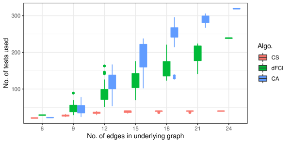
(a) Comparison of number of tests used. For each level of sparsity (number of edges in true graph), we generated 500 graphs, all on 5 nodes. The number of tests required quickly rises for dFCI and CA while CS spends no more than $2\cdot 5(5-1)$ tests. The output of dFCI and CA is not considerably more informative as measured by the mean number of excess edges: CS 0.96, dFCI 0.07, CA 0.81 (average over all levels of sparsity).

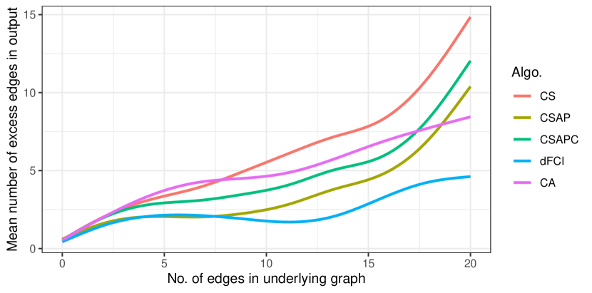
(b) Mean number of excess edges in output graphs for varying numbers of edges (bidirected and directed) in the true graph (all graphs are on 10 nodes), not counting loops.

Figure 3: Comparison of performance.

5 APPLICATION AND SIMULATIONS

When evaluating the performance of a sound screening algoritm, the output graph is guaranteed to be a supergraph of the true parent graph, and we will say that edges that are in the output but not in the true graph are excess edges. For a node in a directed graph, the indegree is the number of directed edges adjacent with and pointed into the node, and the outdegree is the number of directed edges adjacent with and pointed away from the node.

One should note that all our experiments are done using an oracle test, i.e., instead of using real or synthetic data, the algorithms simply query an oracle for each local independence and receive the correct answer. This tests whether or not an algorithm can give good results using an efficient testing strategy (i.e., a low number of queries to the oracle) and therefore it evaluates the algorithms. This approach separates the algorithm from the specific test of local independence and evaluates only the algorithm. As such this is highly unrealistic as we would never have access to an oracle with real data, however, we should think of these experiments as a study of efficiency. The oracle approach to evaluating graphical learning algorithms is common in the DAG-based case, see Spirtes (2010) for an overview.

Also note that the comparison is only made with other constraint-based learning algorithms that can actually solve the problem at hand. Learning methods that assume full observation (such as the Hawkes methods mentioned in Section 2) would generally not output a graph with the correct interpretation even in the oracle case (see the example in Figure 1(b)).

5.1 C. ELEGANS NEURONAL NETWORK

Caenorhabditis elegans is a roundworm in which the network between neurons has been mapped completely (Varshney et al., 2011). We apply our methods to this network as an application to a highly complex network. It consists of 279 neurons which are connected by both non-directional gap junctions and directional chemical synapses. We will represent the former as an unobserved process and the latter as a direct influence which is consistent with the biological system (Varshney et al., 2011). From this network, we sampled subnetworks of 75 neurons each (details in the supplementary material) and computed the output of the CS algorithm. These subsampled networks had on average 1109 edges (including bidirected edges representing unobserved processes, see the supplementary material) and on average 424 directed edges. The output graphs had on average 438 excess edges which is explained by the fact that there are many unobserved nodes in the graphs. To compare the output to the true parent graph, we computed the rank correlation between the indegrees of the nodes in the output graph and the indegrees of the nodes in the true parent graph, and similarly for the outdegree (indegree correlation: 0.94, outdegree correlation: 0.52). Finally, we investigated the method’s ability to identify the observed nodes of highest directed connectivity (i.e., highest in- and outdegrees). The neuronal network of c. elegans is inhomogeneous in the sense that some neurons are extremely highly connected while others are only very sparsely connected. We considered the 15 nodes of highest indegree/outdegree (out of the 75 observed nodes). On average, the CS algorithm placed 13.4 (in) and 9.2 (out) of these 15 among the 15 most connected nodes.

From the output of the CS algorithm, we can find areas of the neuronal network which mediates information from one area to another, e.g., using Corollary 13.

5.2 COMPARISON OF ALGORITHMS

In this section we compare the proposed causal screening algorithms with previously published algorithms that solve similar problems. Mogensen et al. (2018) propose two algorithms, one of which is sure to output the correct graph when an oracle test is available. They note that this complete algorithm is computationally very expensive and adds little extra information, and therefore we will only consider their other algorithm for comparison. We will call this algorithm dynamical FCI (dFCI) as it resembles FCI (Mogensen et al., 2018). dFCI actually solves a harder learning problem (see details in the supplementary material), however, it is computationally infeasible for many problems.

The Causal Analysis (CA) algorithm of Meek (2014) is a simple screening algorithm and we have in this paper argued that it is sound for learning the parent graph under the weaker assumption of ancestral faithfulness. Even though this algorithm uses a large number of tests, it is not guaranteed to provide complete learning as there may be inseparable nodes that are not adjacent (Mogensen et al., 2018; Mogensen and Hansen, 2020).

For the comparison of these algorithms, two aspects are important. As they are all sound, one aspect is the number of excess edges. The other aspect is of course the number of tests needed. The CS and CSAPC algorithms use at most $2n(n-1)$ tests and empirically the CSAP uses roughly the same number as the two former. This makes them feasible in large graphs. The quality of their output is dependent on the sparsity of the true graph, though the CSAP and CSAPC algorithms can deal considerably better with less sparse graphs (Subfigure 3(b)).

6 DISCUSSION

We suggested inexpensive constraint-based methods for learning causal structure based on testing local independence. An important observation is that local independence is asymmetric while conditional independence is symmetric. In a certain sense, this may help when constructing learning algorithms as there is no need of something like an ‘orientation phase’ as in the FCI. This facilitates using very simple methods to give sound causal learning as we do not need the independence structure in full to give interesting output. Simple screening algorithms may be either adaptive or nonadaptive. We note that nonadaptive algorithms may be more robust to false conclusions from statistical tests of local independence.

The amount of information in the output of the screening algorithms depends on the sparsity of the true graph. However, even in examples with very little sparsity interesting structural information can be learned.

We showed that the proposed algorithms have a computational advantage over previously published algorithms within this framework. This makes it feasible to consider causal learning in large networks with unobserved processes. We obtained this gain in efficiency in part by outputting only the directed part of the causal structure. This means that we may be able to answer structural questions, but not questions relating to causal effect estimation.

Acknowledgments

This work was supported by VILLUM FONDEN (research grant 13358). We thank Niels Richard Hansen and the anonymous reviewers for their helpful comments that improved this paper.

Supplementary material

This supplementary material contains additional graph theory, results, and definitions, as well as the proofs of the main paper.

7 GRAPH THEORY

In the main paper, we introduce the class of DGs to represent causal structures. One can represent marginalized DGs using the larger class of DMGs. A directed mixed graph (DMG) is a graph such that any pair of nodes $\alpha,\beta\in V$ is joined by a subset of the edges $\{\alpha\rightarrow\beta,\alpha\leftarrow\beta,\alpha\leftrightarrow\beta\}$.

We say that edges $\alpha\rightarrow\beta$ and $\alpha\leftarrow\beta$ are directed, and that $\alpha\leftrightarrow\beta$ is bidirected. We say that the edge $\alpha\rightarrow\beta$ has a head at $\beta$ and a tail at $\alpha$. $\alpha\leftrightarrow\beta$ has heads at both $\alpha$ and $\beta$. We also introduced a walk $\langle\alpha_{1},e_{1},\alpha_{2},\ldots,\alpha_{n},e_{n},\alpha_{n+1}\rangle$. We say that $\alpha_{1}$ and $\alpha_{n+1}$ are endpoint nodes. A nonendpoint node $\alpha_{i}$ on a walk is a collider if $e_{i-1}$ and $e_{i}$ both have heads at $\alpha_{i}$, and otherwise it is a noncollider. A cycle is a path $\langle\alpha,e_{1},\ldots,\beta\rangle$ composed with an edge between $\alpha$ and $\beta$. We say that $\alpha$ is an ancestor of $\beta$ if there exists a directed path from $\alpha$ to $\beta$. We let $\text{an}(\beta)$ denote the set of nodes that are ancestors of $\beta$. For a node set $C$, we let $\text{an}(C)=\cup_{\beta\in C}\text{an}(\beta)$. By convention, we say that a trivial path (i.e., with no edges) is directed and this means that $C\subseteq\text{an}(C)$.

For DAGs $d$-separation is often used for encoding independences. We use the analogous notion of $\mu$-separation which is a generalization of $\delta$-separation Didelez (2000, 2008); Meek (2014); Mogensen and Hansen (2020).

We use the class of DGs to represent the underlying, data-generating structure. When only parts of the causal system is observed, the class of DMGs can be used to represent marginalized DGs Mogensen and Hansen (2020). This can be done using latent projection Verma and Pearl (1991); Mogensen and Hansen (2020) which is a map that for a DG (or more generally, for a DMG), $\mathcal{D}=(V,E)$, and a subset of observed nodes/processes, $O\subseteq V$, provides a DMG, $m(\mathcal{D},O)$, such that for all $A,B,C\subseteq O$,

$$A\perp_{\mu}B\mid C\ [\mathcal{D}]\Leftrightarrow A\perp_{\mu}B\mid C\ [m(\mathcal{D},O)].$$

See Mogensen and Hansen (2020) for details on this graphical marginalization. We say that two DMGs, $\mathcal{G}_{1}=(V,E_{1}),\mathcal{G}_{2}=(V,E_{2})$, are Markov equivalent if

$$A\perp_{\mu}B\mid C\ [\mathcal{G}_{1}]\Leftrightarrow A\perp_{\mu}B\mid C\ [\mathcal{G}_{2}],$$

for all $A,B,C\subseteq V$, and we let $[\mathcal{G}_{1}]$ denote the Markov equivalence class of $\mathcal{G}_{1}$. Every Markov equivalence class of DMGs has a unique maximal element Mogensen and Hansen (2020), i.e., there exists $\mathcal{G}\in[\mathcal{G}_{1}]$ such that $\mathcal{G}$ is a supergraph of all other graphs in $[\mathcal{G}_{1}]$.

For a DMG, $\mathcal{G}$, we will let $D(\mathcal{G})$ denote the directed part of $\mathcal{G}$, i.e., the DG obtained by deleting all bidirected edges from $\mathcal{G}$.

Proposition 18.

Let $\mathcal{D}=(V,E)$ be a DG, and let $O\subseteq V$. Consider $\mathcal{G}=m(\mathcal{D},O)$. For $\alpha,\beta\in O$ it holds that $\alpha\in\text{an}_{\mathcal{D}}(\beta)$ if and only if $\alpha\in\text{an}_{D(\mathcal{G})}(\beta)$. Furthermore, the directed part of $\mathcal{G}$ equals the parent graph of $\mathcal{D}$ on nodes $O$, i.e., $D(\mathcal{G})=\mathcal{P}_{O}(\mathcal{D})$.

Proof.

Note first that $\alpha\in\text{an}_{\mathcal{D}}(\beta)$ if and only if $\alpha\in\text{an}_{\mathcal{G}}(\beta)$ Mogensen and Hansen (2020). Ancestry is only defined by the directed edges, and it follows that $\alpha\in\text{an}_{\mathcal{G}}(\beta)$ if and only if $\alpha\in\text{an}_{D(\mathcal{G})}(\beta)$. For the second statement, the definition of the latent projection gives that there is a directed edge from $\alpha$ to $\beta$ in $\mathcal{G}$ if and only if there is a directed path from $\alpha$ to $\beta$ in $\mathcal{D}$ such that no nonendpoint node is in $O$. By definition, this is the parent graph, $\mathcal{P}_{O}(\mathcal{D})$. ∎

In words, the above proposition says that if $\mathcal{G}$ is a marginalization (done by latent projection) of $\mathcal{D}$, then the ancestor relations of $\mathcal{D}$ and $D(\mathcal{G})$ are the same among the observed nodes. It also says that our learning target, the parent graph, is actually the directed part of the latent projection on the observed nodes. In the next subsection, we use this to describe what is actually identifiable from the induced independence model of a graph.

7.1 MAXIMAL GRAPHS AND PARENT GRAPHS

Under faithfulness of the local independence model and the causal graph, we know that the maximal DMG is a correct representation of the local independence structure in the sense that it encodes exactly the local independences that hold in the local independence model. From the maximal DMG, one can use results on equivalence classes of DMGs to obtain every other DMG which encodes the observed local independences (Mogensen and Hansen, 2020) and from this graph one can find the parent graph as simply the directed part. However, it may require an infeasible number of tests to output such a maximal DMG. This is not surprising, seeing that the learning target encodes this complete information on local independences.

Assume that $\mathcal{D}_{0}=(V,E)$ is the underlying causal graph and that $\mathcal{G}_{0}=(O,F),O\subseteq V$ is the marginalized graph over the observed variables, i.e., the latent projection of $\mathcal{D}_{0}$. In principle, we would like to output $\mathcal{P}(\mathcal{D}_{0})=D(\mathcal{G}_{0})$, the directed part of $\mathcal{G}_{0}$. However, no algorithm can in general output this graph by testing only local independences as Markov equivalent DMGs may not have the same parent graph. Within each Markov equivalence class of DMGs, there is a unique maximal graph. Let $\bar{\mathcal{G}}$ denote the maximal graph which is Markov equivalent of $\mathcal{G}_{0}$. The DG $D(\bar{\mathcal{G}})$ is a supergraph of $D(\mathcal{G}_{0})$ and we will say that a learning algorithm is complete if it is guaranteed to output $D(\bar{\mathcal{G}})$ as no algorithm testing local independence only can identify anything more than the equivalence class.

8 COMPLETE LEARNING

The CS algorithm provides sound learning of the parent graph of a general DMG under the assumption of ancestral faithfulness. For a subclass of DMGs, the algorithm actually provides complete learning. It is of interest to find sufficient graphical conditions to ensure that the algorithm removes an edge $\alpha\rightarrow\beta$ which is not in the true parent graph. In this section, we state and prove one such condition which can be understood as ‘the true parent set is always found for unconfounded processes’. We let $\mathcal{D}$ denote the output of the CS algorithm.

Proposition 19.

If $\alpha\not\rightarrow_{\mathcal{G}_{0}}\beta$ and there is no $\gamma\in V\setminus\{\beta\}$ such that $\gamma\leftrightarrow_{\mathcal{G}_{0}}\beta$, then $\alpha\not\rightarrow_{\mathcal{D}}\beta$.

Proof.

Let $\mathcal{D}_{1},\mathcal{D}_{2},\ldots,\mathcal{D}_{N}$ denote the DGs that are constructed when running the algorithm by sequentially removing edges, starting from the complete DG, $\mathcal{D}_{1}$. Consider a connecting walk from $\alpha$ to $\beta$ in $\mathcal{G}_{0}$. It must be of the form $\alpha\sim\ldots\sim\gamma\rightarrow\beta$, $\gamma\neq\alpha$. Under ancestral faithfulness, the edge $\gamma\rightarrow\beta$ is in $\mathcal{D}$, thus $\gamma\in\text{pa}_{\mathcal{D}_{i}}(\beta)$ for all $\mathcal{D}_{i}$ that occur during the algorithm, and therefore when $\langle\alpha,\beta\mid\text{pa}_{\mathcal{D}_{i}}(\beta)\setminus\{\alpha\}\rangle$ is tested, the walk is closed. Any walk from $\alpha$ to $\beta$ is of this form, thus also closed, and we have that $\alpha\perp_{\mu}\beta\mid\text{pa}_{\mathcal{D}_{i}}(\beta)$ and therefore $\langle\alpha,\beta\mid\text{pa}_{\mathcal{D}_{i}}(\beta)\setminus\{\alpha\}\rangle\in\mathcal{I}$. The edge $\alpha\rightarrow_{\mathcal{D}_{i}}\beta$ is removed and thus absent in the output graph, $\mathcal{D}$. ∎

9 ANCESTRY PROPAGATION

We state Subalgorithm 4 here.

input : a local independence oracle for $\mathcal{I}^{O}$ and a DG, $\mathcal{D}=(O,E)$

output : a DG on nodes $O$

initialize $E_{r}=\emptyset$ as the empty edge set;

foreach $(\alpha,\beta,\gamma)\in V\times V\times V$ such that $\alpha,\beta,\gamma$ are all distinct do

       if $\alpha\sim_{\mathcal{D}}\beta$, $\beta\rightarrow_{\mathcal{D}}\gamma$, and $\alpha\not\rightarrow_{\mathcal{D}}\gamma$ then

             if $\langle\alpha,\gamma\mid\emptyset\rangle\in\mathcal{I}^{O}$ then

                  update $E_{r}=E_{r}\cup\{\beta\rightarrow\gamma\}$;

             end if

            

       end if

      

end foreach

Update $\mathcal{D}=(V,E\setminus E_{r})$;

return $\mathcal{D}$

Subalgorithm 4 Ancestry propagation

Composing Subalgorithm 1, Subalgorithm 4, and Subalgorithm 2 is referred to as the causal screening, ancestry propagation (CSAP) algorithm. If we use Subalgorithm 3 instead of Subalgorithm 4, we call it the CSAPC algorithm (C for cheap as this does not entail any additional independence tests compared to CS).

10 APPLICATION AND SIMULATIONS

In this section, we provide some additional details about the c. elegans neuronal network and the simulations.

10.1 C. ELEGANS NEURONAL NETWORK

For each connection between two neurons a different number of synapses are present (ranging from 1 to 37). We only consider connections with more than 4 synapses when we define the true underlying network. When sampling the subnetworks, highly connected neurons were sampled with higher probability to avoid a fully connected subnetwork when marginalizing.

10.2 COMPARISON OF ALGORITHMS

As noted in the main paper, the dFCI algorithm solves a strictly harder problem. By using the additional graph theory in the supplementary material, we can understand the output of the dFCI algorithm as a supergraph of the maximal DMG, $\bar{\mathcal{G}}$. There is also a version of the dFCI which is guaranteed to output not only a supergraph of $\bar{\mathcal{G}}$, but the graph $\bar{\mathcal{G}}$ itself. Clearly, from the output of the dFCI algorithm, one can simply take the directed part of the output and this is a supergraph of the underlying parent graph.

11 PROOFS

In this section, we provide the proofs of the result in the main paper.

Proof of Proposition 5.

Let $\mathcal{D}$ denote the causal graph. Assume first that $\alpha\not\rightarrow_{\mathcal{D}}\beta$. Then $g^{\beta\alpha}$ is identically zero over the observation interval, and it follows directly from the functional form of $\lambda_{t}^{\beta}$ that $\alpha\not\rightarrow\beta\mid V\setminus\{\alpha\}$. This shows that the local independence model satisfies the pairwise Markov property with respect to $\mathcal{D}$.

If instead $g^{\beta\alpha}\neq 0$ over $J$, there exists $r\in J$ such that $g^{\beta\alpha}(r)\neq 0$. From continuity of $g^{\beta\alpha}$ there exists a compact interval of positive measure, $I\subseteq J$, such that $\inf_{s\in I}(g^{\beta\alpha}(s))\geq g_{\min}^{\beta\alpha}$ and $g_{\min}^{\beta\alpha}>0$. Let $i_{0}$ and $i_{1}$ denote the endpoints of this interval, $i_{0}<i_{1}$. We consider now the events

$$D_{k}=(N_{T-i_{0}}^{\alpha}-N_{T-i_{1}}^{\alpha}=k,N_{T}^{\gamma}=0\text{ for all }\gamma\in V\setminus\{\alpha\})$$

$k\in\mathbb{N}_{0}$. Then under Assumption 4, for all $k$

$$\lambda_{T}^{\beta}\mathds{1}_{D_{k}}\geq\mathds{1}_{D_{k}}\int_{I}g^{\beta\alpha}(T-s)\ \mathrm{d}N_{s}^{\alpha}\geq g_{\min}^{\beta\alpha}\cdot k\cdot\mathds{1}_{D_{k}}.$$

Assume for contradiction that $\beta$ is locally independent of $\alpha$ given $V\setminus\{\alpha\}$. Then $\lambda_{T}^{\beta}=\text{E}(\lambda_{T}^{\beta}\mid\mathcal{F}_{T}^{V})=\text{E}(\lambda_{T}^{\beta}\mid\mathcal{F}_{T}^{V\setminus\{\alpha\}})$ is constant on $\cup_{k}D_{k}$ and furthermore $\text{P}(D_{k})>0$ for all $k$. However, this contradicts the above inequality when $k\rightarrow\infty$. ∎

Proof of Proposition 12.

Let $\mathcal{D}$ denote the DG which is output by the algorithm. We should then show that $\mathcal{P}(\mathcal{D}_{0})\subseteq\mathcal{D}$. Assume that $\alpha\rightarrow_{\mathcal{P}(\mathcal{D}_{0})}\beta$. In this case, there is a directed path from $\alpha$ to $\beta$ in $\mathcal{D}_{0}$ such that no nonendpoint node on this directed walk is in $O$ (the observed coordinates). Therefore for any $C\subseteq O\setminus\{\alpha\}$ there exists a directed $\mu$-connecting walk from $\alpha$ to $\beta$ in $\mathcal{D}_{0}$ and by ancestral faithfulness it follows that $\langle\alpha,\beta\mid C\rangle\notin\mathcal{I}$. The algorithm starts from the complete directed graph, and the above means that the directed edge from $\alpha$ to $\beta$ will not be removed. ∎

Proof of Corollary 13.

Consider some directed path from $\alpha$ to $\beta$ in $\mathcal{D}_{0}$ on which no node is in $C$. Then there is also a directed path from $\alpha$ to $\beta$ on which no nodes is in $C$ in the graph $\mathcal{P}(\mathcal{D}_{0})$, and therefore also in the output graph using Proposition 12. ∎

Proof of Proposition 15.

Assume that there is a $\mu$-connecting walk from $\alpha$ to $\beta$ given $\{\beta\}$. If this walk has no colliders, then it is a directed trek, or can be reduced to one. Otherwise, assume that $\gamma$ is the collider which is the closest to the endpoint $\alpha$. Then $\gamma\in\text{an}(\beta)$, and composing the subwalk from $\alpha$ to $\gamma$ with the directed path from $\gamma$ to $\beta$ gives a directed trek, or it can be reduced to one. On the other hand, assume there is a directed trek from $\alpha$ to $\beta$. This is $\mu$-connecting from $\alpha$ to $\beta$ given $\{\beta\}$. ∎

Proof of Proposition 17.

Assume $\beta\rightarrow_{\mathcal{P}(\mathcal{D}_{0})}\gamma$. Subalgorithms 1 and 2 are both simple screening algorithms, and they will not remove this edge. Assume for contradiction that $\beta\rightarrow\gamma$ is removed by Subalgorithm 3. Then there must exist $\alpha\neq\beta,\gamma$ and a directed trek from $\alpha$ to $\beta$ in $\mathcal{D}_{0}$. On this directed trek, $\gamma$ does not occur as this would imply a directed trek either from $\alpha$ to $\gamma$ or from $\beta$ to $\alpha$, thus implying $\alpha\rightarrow_{\mathcal{D}}\gamma$ or $\beta\rightarrow_{\mathcal{D}}\alpha$, respectively ($\mathcal{D}$ is the output graph of Subalgorithm 1). As $\gamma$ does not occur on the trek, composing this trek with the edge $\beta\rightarrow\gamma$ would give a directed trek from $\alpha$ to $\gamma$. By faithfulness, $\langle\alpha,\gamma\mid\gamma\rangle\notin\mathcal{I}$, and this is a contradiction as $\alpha\rightarrow\gamma$ would not have been removed during Subalgorithm 1.

We consider instead CSAP. Assume for contradiction that $\beta\rightarrow\gamma$ is removed during Subalgorithm 4. There exists in $\mathcal{D}_{0}$ either a directed trek from $\alpha$ to $\beta$ or a directed trek from $\beta$ to $\alpha$. If $\gamma$ is on this trek, then $\gamma$ is not $\mu$-separated from $\alpha$ given the empty set (recall that there are loops at all nodes, therefore also at $\gamma$), and using faithfulness we conclude that $\gamma$ is not on this trek. Composing it with the edge $\beta\rightarrow\gamma$ would give a directed trek from $\alpha$ to $\gamma$ and using faithfulness we obtain a contradiction. ∎

References

- Aalen (1987) Odd O. Aalen. Dynamic modelling and causality. Scandinavian Actuarial Journal, pages 177–190, 1987.
- Achab et al. (2017) Massil Achab, Emmanuel Bacry, Stéphane Gaïffas, Iacopo Mastromatteo, and Jean-François Muzy. Uncovering causality from multivariate Hawkes integrated cumulants. In Proceedings of the 34th International Conference on Machine Learning (ICML), 2017.
- Bacry et al. (2015) Emmanuel Bacry, Iacopo Mastromatteo, and Jean-François Muzy. Hawkes processes in finance. Market Microstructure and Liquidity, 1(1), 2015.
- Colombo et al. (2012) Diego Colombo, Marloes H. Maathuis, Markus Kalisch, and Thomas S. Richardson. Learning high-dimensional directed acyclic graphs with latent and selection variables. The Annals of Statistics, 40(1):294–321, 2012.
- Commenges and Gégout-Petit (2009) Daniel Commenges and Anne Gégout-Petit. A general dynamical statistical model with causal interpretation. Journal of the Royal Statistical Society. Series B (Statistical Methodology), 71(3):719–736, 2009.
- Daley and Vere-Jones (2003) Daryl J. Daley and David D. Vere-Jones. An introduction to the theory of point processes. New York: Springer, 2nd edition, 2003.
- Didelez (2000) Vanessa Didelez. Graphical Models for Event History Analysis based on Local Independence. PhD thesis, Universität Dortmund, 2000.
- Didelez (2008) Vanessa Didelez. Graphical models for marked point processes based on local independence. Journal of the Royal Statistical Society, Series B, 70(1):245–264, 2008.
- Eichler (2012) Michael Eichler. Graphical modelling of multivariate time series. Probability Theory and Related Fields, 153(1):233–268, 2012.
- Eichler (2013) Michael Eichler. Causal inference with multiple time series: Principles and problems. Philosophical Transactions of the Royal Society, 371(1997):1–17, 2013.
- Eichler and Didelez (2010) Michael Eichler and Vanessa Didelez. On Granger causality and the effect of interventions in time series. Lifetime Data Analysis, 16(1):3–32, 2010.
- Eichler et al. (2017) Michael Eichler, Rainer Dahlhaus, and Johannes Dueck. Graphical modeling for multivariate Hawkes processes with nonparametric link functions. Journal of Time Series Analysis, 38:225–242, 2017.
- Etesami et al. (2016) Jalal Etesami, Negar Kiyavash, Kun Zhang, and Kushagra Singhal. Learning network of multivariate Hawkes processes: A time series approach. In Proceedings of the 32nd Conference on Uncertainty in Artificial Intelligence (UAI), 2016.
- Foygel et al. (2012) Rina Foygel, Jan Draisma, and Mathias Drton. Half-trek criterion for generic identifiability of linear structural equation models. The Annals of Statistics, 40(3):1682–1713, 2012.
- Jovanović et al. (2015) Stojan Jovanović, John Hertz, and Stefan Rotter. Cumulants of Hawkes point processes. Physical Review E, 91(4), 2015.
- Laub et al. (2015) Patrick J. Laub, Thomas Taimre, and Philip K. Pollett. Hawkes processes. 2015. URL https://arxiv.org/pdf/1507.02822.pdf.
- Liniger (2009) Thomas Josef Liniger. Multivariate Hawkes processes. PhD thesis, ETH Zürich, 2009.
- Luo et al. (2015) Dixin Luo, Hongteng Xu, Yi Zhen, Xia Ning, Hongyuan Zha, Xiaokang Yang, and Wenjun Zhang. Multi-task multi-dimensional Hawkes processes for modeling event sequences. In Proceedings of the 24th International Joint Conference on Artificial Intelligence (IJCAI), 2015.
- Maathuis et al. (2019) Marloes Maathuis, Mathias Drton, Steffen Lauritzen, and Martin Wainwright. Handbook of graphical models. Chapman & Hall/CRC handbooks of modern statistical methods, 2019.
- Magliacane et al. (2016) Sara Magliacane, Tom Claassen, and Joris M. Mooij. Ancestral causal inference. In Proceedings of the 29th Conference on Neural Information Processing Systems (NIPS), 2016.
- Meek (2014) Christopher Meek. Toward learning graphical and causal process models. In CI’14 Proceedings of the UAI 2014 Conference on Causal Inference: Learning and Prediction, 2014.
- Mogensen and Hansen (2020) Søren Wengel Mogensen and Niels Richard Hansen. Markov equivalence of marginalized local independence graphs. The Annals of Statistics, 48(1), 2020.
- Mogensen et al. (2018) Søren Wengel Mogensen, Daniel Malinsky, and Niels Richard Hansen. Causal learning for partially observed stochastic dynamical systems. In Proceedings of the 34th conference on Uncertainty in Artificial Intelligence (UAI), 2018.
- Pearl (2009) Judea Pearl. Causality. Cambridge University Press, 2009.
- Peters et al. (2017) Jonas Christopher Peters, Dominik Janzing, and Bernhard Schölkopf. Elements of causal inference, foundations and learning algorithms. MIT Press, 2017.
- Røysland (2012) Kjetil Røysland. Counterfactual analyses with graphical models based on local independence. The Annals of Statistics, 40(4):2162–2194, 2012.
- Spirtes (2001) Peter Spirtes. An anytime algorithm for causal inference. In Proceedings of the 8th International Workshop on Artificial Intelligence and Statistics (AISTATS), 2001.
- Spirtes (2010) Peter Spirtes. Introduction to causal inference. Journal of Machine Learning Research, 11, 2010.
- Spirtes et al. (2000) Peter Spirtes, Clark Glymour, and Richard Scheines. Causation, Prediction, and Search. MIT Press, 2000.
- Tan et al. (2018) Xi Tan, Vinayak Rao, and Jennifer Neville. Nested CRP with Hawkes-Gaussian processes. In Proceedings of the 21st International Conference on Artificial Intelligence and Statistics (AISTATS), 2018.
- Trouleau et al. (2019) William Trouleau, Jalal Etesami, Matthias Grossglauser, Negar Kiyavash, and Patrick Thiran. Learning Hawkes processes under synchronization noise. In Proceedings of the 36th International Conference on Machine Learning (ICML), 2019.
- Varshney et al. (2011) Lav R. Varshney, Beth L. Chen, Eric Paniagua, David H. Hall, and Dmitri B. Chklovskii. Structural properties of the Caenorhabditis elegans neuronal network. PLoS Computational Biology, 7(2), 2011.
- Verma and Pearl (1991) Thomas Verma and Judea Pearl. Equivalence and synthesis of causal models. Technical Report R-150, University of California, Los Angeles, 1991.
- Xu et al. (2016) Hongteng Xu, Mehrdad Farajtabar, and Hongyuan Zha. Learning Granger causality for Hawkes processes. In Proceedings of the 33rd International Conference on Machine Learning (ICML), 2016.
- Xu et al. (2018) Hongteng Xu, Dixin Luo, Xu Chen, and Lawrence Carin. Benefits from superposed Hawkes processes. In Proceedings of the 21st International Conference on Artificial Intelligence and Statistics (AISTATS), 2018.
- Zhalama et al. (2017a) Zhalama, Jiji Zhang, Frederick Eberhardt, and Wolfgang Mayer. SAT-based causal discovery under weaker assumptions. In Proceedings of the 33th Conference on Uncertainty in Artificial Intelligence (UAI), 2017a.
- Zhalama et al. (2017b) Zhalama, Jiji Zhang, and Wolfgang Mayer. Weakening faithfulness: Some heuristic causal discovery algorithms. International Journal of Data Science and Analytics, 3:93–104, 2017b.
- Zhang (2008) Jiji Zhang. On the completeness of orientation rules for causal discovery in the presence of latent confounders and selection bias. Artificial Intelligence, 172:1873–1896, 2008.
- Zhang and Spirtes (2008) Jiji Zhang and Peter Spirtes. Detection of unfaithfulness and robust causal inference. Minds & Machines, 18:239–271, 2008.
- Zhou et al. (2013a) Ke Zhou, Hongyuan Zha, and Le Song. Learning triggering kernels for multi-dimensional Hawkes processes. In Proceedings of the 30th International Conference on Machine Learning (ICML), 2013a.
- Zhou et al. (2013b) Ke Zhou, Hongyuan Zha, and Le Song. Learning social infectivity in sparse low-rank networks using multi-dimensional Hawkes processes. In Proceedings of the 16th International Conference on Artificial Intelligence and Statistics (AISTATS), 2013b.