Two Long-Period Cataclysmic Variable Stars: ASASSN-14ho and V1062 Cyg

Abstract

We report spectroscopy and photometry of the cataclysmic variable stars ASASSN-14ho and V1062 Cyg. Both are dwarf novae with spectra dominated by their secondary stars, which we classify approximately as K4 and M0.5, respectively. Their orbital periods, determined mostly from the secondary stars’ radial velocities, proved to be nearly identical, respectively $350.14\pm 0.15$ and $348.25\pm 0.60$ min. The H$\alpha$ emission line in V1062 Cyg displays a relatively sharp emission component that tracks the secondary’s motion, which may arise on the irradiated face of the secondary; this is not often seen and may indicate an unusually strong flux of ionizing radiation. Both systems exhibit double-peaked orbital modulation consistent with ellipsoidal variation from the changing aspect of the secondary. We model these variations to constrain the orbital inclination $i$, and estimate approximate component masses based on $i$ and the secondary velocity amplitude $K_{2}$.

1 Introduction

Cataclysmic variable stars (CVs) are binary stars in which a white dwarf primary accretes matter from a more extended secondary star via Roche lobe overflow. The accreting matter usually forms a disk around the primary. A good overview of CVs is presented in Warner (1995).

Dwarf novae (DN), one of the most common types of CV, are weakly or non-magnetic systems which can spontaneously go from quiescence into outburst, a more luminous state corresponding to a brightening of several magnitudes. DN outbursts are thought to be caused by the rapid release of gravitational potential energy triggered by instabilities in the accretion disk. At longer orbital periods, the quiescent spectra of DN are often dominated by the spectrum of a late-type secondary (Warner, 1995).

DN systems in which the secondary star is the dominant flux contributor often show a modulation in the light curve caused by the tidal distortions in the secondary star (Barwig & Schoembs, 1983). The projection effects cause two maxima per orbital period at the quadrature phases, and gravity darkening causes the side of the secondary facing the white dwarf to appear darker than the back side, resulting in unequal minima (Bochkarev et al., 1979).

This work focuses on two DN systems: ASASSN-14ho and V1062 Cyg. We obtained optical spectroscopy and photometry of these systems in order to determine their orbital periods and estimate the spectral types of their secondary stars and the binary system parameters.

ASSASN-14ho (RA = 06${}^{\text{h}}$30${}^{\text{m}}$27.3${}^{\text{s}}$, Dec = $-65^{\circ}$29^′′50.2^′, J2000) was announced as a CV in outburst following observations taken of the system on the du Pont 2.5 m spectrograph at the Las Campanas Observatory in September 2014 (Prieto et al., 2014). The system had quiescent brightness of $V=15.4$ on 2014 Sept. 9 and reached $V=10.92$ on 2014 Sept. 11 Sept before declining. A previous outburst had been seen in 2009 by the Catalina Real Time Transient Survey (Drake et al., 2009). Inverting the Gaia Data Release 2 (DR2) parallax (Gaia Collaboration et al., 2016, 2018) gives a distance estimate of $331\pm 3$ pc.

V1062 Cyg (RA = $21^{\textrm{h}}08^{\textrm{m}}12.20^{\textrm{s}}$, Dec = $+36^{\circ}49^{\prime\prime}27.7^{\prime}$, J2000) was first reported by Hoffmeister (1965), with a magnitude range of 15.5 - 18 mag. Despite having since appeared in several CV catalogs, the system has apparently never been studied in detail and its orbital period remained unknown. The inverse of its Gaia DR2 parallax is $840\,(+95,-78)$ pc.

We describe our observations, instruments, and analysis in Section 2. In Sections 3 and 4 we present our results for ASSASN-14ho and V1062 Cyg, respectively. Finally, our conclusions and discussion are presented in Section 5.

Table 1: Radial Velocities of ASASSN-14ho

Time	$v_{\rm abs}$	$v_{\rm emn}$
	(km s-1)	(km s-1)
57794.3628	$318\pm 10$	$-45\pm 13$
57794.3698	$319\pm 11$	$-35\pm 14$
57794.3771	$269\pm 12$	$-55\pm 16$
57794.3841	$268\pm 10$	$-39\pm 15$
57794.3984	$201\pm 11$	$-62\pm 14$
57794.4054	$154\pm 11$	$-43\pm 16$
57794.4124	$128\pm 15$	$-6\pm 16$
57794.4193	$63\pm 13$	$-7\pm 21$
57794.4287	$41\pm 30$	$56\pm 20$
57794.4357	$-38\pm 15$	$80\pm 22$
57794.4427	$-45\pm 12$	$72\pm 18$
57794.4497	$-98\pm 12$	$63\pm 23$
57794.4594	$-131\pm 13$	$11\pm 26$
57794.4664	$-143\pm 11$	$66\pm 21$
57794.4734	$-152\pm 12$	$90\pm 23$
57794.4804	$-173\pm 10$	$76\pm 27$
57794.4895	$-148\pm 13$	$123\pm 20$
57794.4964	$-145\pm 12$	$119\pm 21$
57794.5034	$-140\pm 11$	$70\pm 18$
57794.5104	$-106\pm 28$	$108\pm 16$
57794.5205	$-67\pm 11$	$101\pm 17$
57794.5275	$-20\pm 19$	$100\pm 19$
57794.5345	$18\pm 12$	$57\pm 25$
57794.5415	$75\pm 14$	$\cdots$
57794.5498	$125\pm 13$	$\cdots$
57794.5572	$112\pm 34$	$62\pm 26$
57794.5642	$208\pm 15$	$\cdots$
57794.5712	$237\pm 19$	$\cdots$
57796.2883	$300\pm 11$	$-34\pm 16$
57796.2953	$311\pm 9$	$-26\pm 16$
57796.3023	$302\pm 9$	$-78\pm 16$
57796.3093	$316\pm 10$	$-46\pm 17$
57796.3173	$290\pm 9$	$-43\pm 21$
57796.3243	$271\pm 10$	$-24\pm 19$
57796.3313	$246\pm 10$	$-40\pm 20$
57796.3383	$218\pm 10$	$-72\pm 21$
57796.3500	$164\pm 11$	$-59\pm 24$
57796.3570	$104\pm 9$	$-37\pm 21$
57797.2745	$295\pm 10$	$-31\pm 20$
57797.2862	$267\pm 10$	$-33\pm 17$
57797.2978	$254\pm 8$	$-36\pm 18$
57799.2718	$150\pm 8$	$\cdots$
57799.2802	$94\pm 8$	$\cdots$

Table 2: Radial Velocities of V1062 Cyg

Time	$v_{\rm abs}$	H$\alpha$ wing	H$\alpha$ peak
(km s-1)	(km s-1)	(km s-1)
57928.7553	$139\pm 48$	$\cdots$	$112\pm 34$
57928.7640	$83\pm 33$	$\cdots$	$92\pm 23$
57928.7727	$171\pm 30$	$\cdots$	$49\pm 22$
57928.7814	$158\pm 32$	$\cdots$	$94\pm 20$
57928.7931	$110\pm 31$	$-185\pm 39$	$57\pm 22$
57928.8074	$146\pm 26$	$-202\pm 27$	$81\pm 15$
57928.8602	$-107\pm 30$	$-45\pm 31$	$-60\pm 23$
57928.8745	$-163\pm 29$	$12\pm 32$	$-76\pm 22$
57928.8888	$-207\pm 25$	$-36\pm 25$	$-147\pm 16$
57928.9031	$-227\pm 23$	$-7\pm 30$	$-157\pm 17$
57928.9174	$-213\pm 23$	$18\pm 31$	$-153\pm 18$
57928.9316	$-204\pm 29$	$72\pm 36$	$-66\pm 20$
57928.9459	$-99\pm 18$	$3\pm 28$	$-85\pm 15$
57928.9602	$-33\pm 25$	$-43\pm 33$	$-90\pm 21$
57929.8507	$-160\pm 28$	$34\pm 38$	$-221\pm 19$
57929.8684	$-215\pm 22$	$81\pm 24$	$-143\pm 14$
57929.8862	$\cdots$	$\cdots$	$-80\pm 31$
57930.7428	$\cdots$	$-147\pm 30$	$\cdots$
57930.7605	$72\pm 35$	$-186\pm 25$	$31\pm 30$
57930.7783	$-81\pm 44$	$\cdots$	$\cdots$
57930.7960	$-153\pm 46$	$-75\pm 34$	$-172\pm 33$
57930.8137	$-189\pm 29$	$-41\pm 30$	$-224\pm 20$
57930.8331	$-196\pm 33$	$67\pm 25$	$-184\pm 21$
57930.9336	$93\pm 27$	$-198\pm 19$	$68\pm 23$

Table 3: Photometric Observations of ASASSN-14ho

Date	Time	Exp	N	Airmass
	(UTC)	(s)		Start	End
2017-02-11	18:44:21	10.0	450	1.2079	1.1954
2017-02-11	19:59:41	15.0	320	1.1954	1.2426
2017-02-11	21:20:10	25.0	355	1.2429	1.5361

Table 4: Photometric Observations of V1062 Cyg

Date	Time	Exp	N	Airmass
	(UTC)	(s)		Start	End
2017-06-27	05:15:57	60.0	360	1.991	1.030
2017-06-28	05:03:12	60.0	360	2.094	1.023

2 Methods

2.1 Observations

Our observations of ASASSN-14ho were taken in February 2017 at the South African Astronomical Observatory (SAAO) near Sutherland. Observations of V1062 Cyg were taken in June 2017 at MDM Observatory, on Kitt Peak, Arizona.

Our spectra of ASASSN-14ho were taken with the Spectrograph Upgrade – Newly Improved Cassegrain (SpUpNIC) instrument (Crause et al., 2016) mounted on the SAAO 1.9 m telescope. We used the G6 grating (blazed for 4600 Å) which gave a dispersion of 1.36 Å px^-1. A 1.35-arcsec slit and a grating angle of 11.75^∘ yielded a resolving power of 1000 from 4200 to 7000 Å. We obtained 43 spectra of ASASSN-14ho, mostly 600-s exposures, over five days, for a total integration time of just over 7.5 hr. Table 1 gives the times of observation and radial velocities derived from the spectra (described in Section 2.3).

The V1062 Cyg spectra were taken with the modspec spectrograph on the 2.4 m Hiltner telescope. We used a 600 mm^-1 5000 Å blazed grating and a $2048\times 2048$ 24-micron pixel SITe CCD, which gave a wavelength range of 4300 Å to 7500 Å and a resolution of 3.4 Å. Table 2 gives the times of observation and radial velocities derived from the spectra.

The photometry of ASASSN-14ho is from the Sutherland High Speed Optical Camera (SHOC; Coppejans et al. 2013) on the SAAO 1.0 m telescope. The instrument uses a back-illuminated frame transfer CCD with a 6.76 ms dead time. The system offers a $2.85^{\prime}\times 2.85^{\prime}$ field of view with a plate scale of $0.668^{\prime\prime}\,\text{px}^{-1}$ in the $4\times 4$ binning mode. Our observations, all from 2017 Feb. 11, consist of 1125 unfiltered frames obtained over five hours. Table 3 gives the times of observations, length of exposure, number of frames taken, and airmass.

Our photometry of V1062 Cyg was taken with an Andor Ikon DU-937N camera on the MDM 1.3 m McGraw-Hill Telescope. The camera has $512\times 512$ 13 $\mu\textrm{m}^{2}$ pixels which gave a $2.32^{\prime}\times 2.32^{\prime}$ field of view (Thorstensen, 2013). Over the course of two nights, 720 frames were taken for a total integration time of twelve hours. Table 4 gives the times of observations, length of exposure, number of frames taken, and airmass.

2.2 Data Reduction

We reduced our spectra using procedures broadly similar to those outlined in Thorstensen et al. (2016). We used IRAF for bias and flat field corrections. For the SAAO spectra we extracted background-subtracted 1-dimensional spectra using the IRAF apall task, and applied wavelength calibrations derived from Cu-Ar arc spectra interleaved with the stellar exposures. For the MDM data, we extracted the spectra using a local implementation of the algorithm given by Horne (1986), and a wavelength scale derived by rigidly shifting a master pixel-to-wavelength solution using the $\lambda 5577$ airglow line as a fiducial. At both observatories we derived a flux calibration using observations of standard stars taken during the run.

Both the SAAO SHOC and the MDM Andor camera write 3-dimensional data cubes. To process these we used python scripts to (1) create average bias images and flat field frames from exposures of the twilight sky (2) subtract the bias and divide by the flat field, and (3) derive barycentric times of the exposure centers. We then split the individual frames from the data cube and measured the magnitudes of the program object and several comparison stars using the aperture photometry task in the IRAF implementation of DAOPHOT (Stetson, 1987), and finally compiled the differential magnitudes into a time series. The uncertainties in our program star measurements were estimated from the scatter in the differential magnitudes of apparently constant stars of similar brightness.

Our data cannot be transformed accurately to a standard passband because the SAAO data were taken unfiltered, and the filter used at MDM was intended only to mitigate scattered moonlight (passing $\lambda>4200$ Å). However, we did transform to approximate $V$ magnitude by adding the $V$ magnitudes of our comparison stars to the differential magnitudes. These pseudo-$V$ magnitudes should not be very far off, since in both systems the late-type secondary star dominates the light; the color mismatch between the CV and the comparison star is therefore unlikely to be severe.

2.3 Analysis

We measured radial velocities of the secondary stars using the cross-correlation technique of Tonry & Davis (1979). For the template spectrum, we used the average of 76 spectra of G and K type stars, taken with the Hiltner telescope and modspec in the same configuration used here for V1062 Cyg, that had been shifted to zero apparent velocity prior to averaging.

To measure emission-line velocities, we used a convolution technique developed by Schneider & Young (1980), in which the line profile is convolved with an odd function and the zero of the convolution is taken as a measure of the line center. For the odd function, we used either the derivative of a gaussian (‘dgau’ for short) or the sum of positive and negative Gaussians, offset by a selectable width (‘gau2’). In both cases, only the H$\alpha$ line gave usable velocities.

To search for periods, we fit general least-squares sinusoids to the radial velocities at each frequency in a dense grid of trial frequencies. In both stars studied here, the adopted orbital frequency had by far the lowest scatter aound the best fit, and there was no ambiguity in the daily cycle count. We fit the radial velocities with functions of the form

$$v(t)=K\sin\left(\frac{2\pi(t-T_{0})}{P}\right)+\gamma$$

where $P$ is the orbital period and $T_{0}$ is an epoch of blue-to-red crossing chosen to be near the center of the time series. If the velocities faithfully trace the motion of one component, then $\gamma$ will be the systemic radial velocity and $K$ will be the line-of-sight component of that star’s orbital velocity. We used a Monte Carlo simulation to estimate the uncertainties in the parameters of our best-fitting sinusoid.

To estimate the secondary stars’ spectral types, we began by shifting our individual flux-calibrated spectra to the secondary’s rest frame and averaging them. We then subtracted spectra of known spectral type taken from the same instrument, varying the spectral type and normalization with the aim of retrieving a smooth continuum as judged by eye. This resulted in a range of possible classifications and V-band magnitudes for the secondary.

To display the spectrum as a function of orbital phase, we set up a grid of 100 evenly-spaced fiducial phases around the orbital cycle, and computed average spectra for each phase. Weights for the spectra near each fiducial phase were computed using a Gaussian weighting function, with a standard deviation of $0.03$ cycles. The spectra were rectified (divided by a continuum fit) and cleaned of obvious artifacts before being averaged. We then stacked the phase-averages into a 2-dimensional image, and generated greyscale figures from these.

The light curves of both objects showed two peaks per orbit and unequal minima, as expected from the changing aspect of a tidally distorted secondary star. To explore this, we used a modeling program described by Thorstensen & Armstrong (2005). The program models the Roche-lobe-filling secondary star as a 500-sided polyhedron and computes the $V$-band light curve for the source as observed from Earth. The model parameters are the (assumed known) orbital period, the masses of both stars, the orbital inclination $i$, the secondary’s effective temperature $T_{\rm eff}$, limb- and gravity-darkening coefficients, the distance and reddening of the system, and an assumed flat (in flux per unit wavelength $F_{\lambda}$) ‘extra light’ contribution from the primary and accretion structures. Our estimates of $T_{\rm eff}$ and the ‘extra light’ are guided by the spectral decompositions used to estimate the secondary’s spectral type. For all calculations we used a linear limb-darkening coefficient of 0.78, from the tabulations of Claret et al. (2012) for $T_{\rm eff}=4500$ K and the Kepler passband, which is similar to our observed bands.

From $P$ and the secondary star’s velocity semiamplitude $K_{2}$, we compute the mass function

$$f=\frac{(M_{1})^{3}}{(M_{1}+M_{2})^{2}}\sin^{3}({i})=\frac{P}{2\pi G}(K_{2})^{3}.$$

We use this to constrain the secondary star’s mass $M_{2}$ by estimating a range of plausible inclinations $i$ from the light curve model fits, and assuming that the white dwarf mass $M_{1}$ lies in a reasonable range (Kepler et al., 2007; Ritter & Burkert, 1986; Schreiber et al., 2016). Sections 3.3 and 4.3 detail this process for for ASASSN-14ho and V1062 Cyg respectively.

3 ASASSN-14ho Results

3.1 Period and Radial Velocities

The absorption line radial velocities are modulated with an unambiguous period of $350.14\,\pm\,0.15$ min, which we adopt as $P_{\rm orb}$. The H$\alpha$ line is double-peaked with a full width at half-maximum of $\sim 31$ Å. We measured its radial velocity using a ‘gau2’ convolution function with a separation of 44 Å, which emphasized the steep sides and wings of the line. The emission velocities showed modulation at essentially the same period as the absorption, but with greater scatter. Table 5 gives parameters of sinusoidal fits to the emission and absorption velocities, and Figure 1 shows the velocities plotted as a function of phase, along with the best-fit sinusoids.

Table 5: Fits to Radial Velocities

Data set	$T_{0}$	$P$	$K$	$\gamma$	$N$	RMS
		(d)	(km s-1)	(km s-1)		(km s-1)
ASASSN-14ho absorption	2457794.5417(10)	0.24316(10)	236(5)	69(4)	43	13
ASASSN-14ho emission	2457794.436(7)	[0.24316]	78(10)	29(8)	37	22
V1062 Cyg absorption	2457929.931(2)	0.2418(5)	184(7)	$-$32(5)	22	24
V1062 Cyg H$\alpha$ cores	57929.927(9)	0.2418	126(20)	$-37(17)$	23	41
V1062 Cyg H$\alpha$ wings	57929.818(7)	0.2418	129(19)	$-88(15)$	18	38

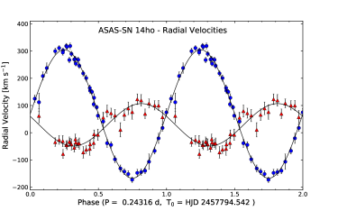
Figure 1: ASASSN-14ho radial velocities folded on the orbital period, with one cycle repeated once for clarity. The blue circles are absorption-line velocties of the secondary star, and the red triangles are velocities of the H$\alpha$ emission line wings.

The systemic radial velocity $\gamma$ derived from the absorption lines differs by 42 km s^-1 from the value from the emission lines. We do not think this discrepancy is significant, because the emission line velocities do not necessarily trace the white dwarf motion (North et al., 2002). If the emission originated directly from the white dwarf, we would expect an emission-absorption phase offset of 0.5 cycle. Our fitted sinusoids show a difference of $0.56\pm 0.03$ cycles, suggesting that the emission from the accretion disk does not track the white dwarf’s position exactly. The emission velocities are uncertain enough that we are reluctant to use them to compute a mass ratio.

Figure 2 shows a single-trailed plot of the spectral features of ASASSN-14ho, centered on the H$\alpha$ emission line. The H$\alpha$ profile is complex, but has the distinct double-peaked structure characteristic of an accretion disk.

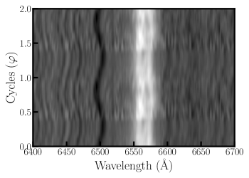
Figure 2: Single-trailed spectrum on ASASSN-14ho, centered on the H$\alpha$ emission line.

3.2 Spectral Type

We find the secondary’s spectral type to be near K4V, with an estimated uncertainty of $\pm 2$ subclasses. The secondary star contributes most of the light in the visible (Fig. 3). The subtracted spectrum is characterized by a fairly flat continuum with broad hydrogen emission lines, typical of dwarf novae at minimum light (Warner, 1995).

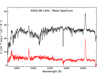
Figure 3: Average spectrum of ASASSN-14ho (black) together with the the spectrum after subtraction (red) of a scaled spectrum of the K4V star Gliese 570a. The individual spectra of ASASSN-14ho were shifted to the rest frame of the secondary star before they were summed.

3.3 Photometry and Stellar Parameters

Figure 4 shows our photometry folded on the period and phase determined in Section 3.1. As noted earlier, we transformed our instrumental magnitudes to rough apparent $V$ magnitudes using $V=15.25$ for the comparison star , taken from the AAVSO Photometric All-Sky Survey (APASS) catalog (Henden et al., 2015). The light curve shows an obvious modulation with two peaks per orbit and unequal minima, as expected from a tidally-distorted secondary (so-called ellipsoidal variation), and no evidence of an eclipse. The red curve in Fig. 4 shows a light curve generated by the light-curve modeling program described earlier. We could not fit all the features in the light curve, such as the extra brightness near phase zero, with perfect fidelity. Therefore, we did not attempt a formal best fit, but adjusted the fit parameters by hand. The fit shown has $M_{1}=1.00$ and $M_{2}=0.28$ M_⊙, $i=52$ degrees, a secondary effective temperature of 4200 kelvin, and extra light equivalent to $F_{\lambda}=5\times 10^{-16}$ erg s^-1 cm^-2 Å^-1, which gives a reddening-corrected distance nearly identical to the inverse of the Gaia DR2 parallax, and matches the observed mass function. The amplitude of the modeled curve is influenced mostly by the inclination, the estimated contribution from the disk, constant “extra light” term, and the gravity darkening coefficient. With the last two factors held constant, we found reasonable fits in the range $i=52\pm 5$ degrees. Varying $M_{2}$ mostly affects the normalization, because the Roche lobe radius scales roughly as $M_{2}^{1/3}$.

In Figure 5, we show the constraints on $M_{1}$ and $M_{2}$ set by the velocity amplitude, for several inclination angles consistent with the light curve. The masses are sensitive to small changes in inclination. The box in the figure represents a rough range of reasonable masses for both components. If our inclination estimate is correct, the white dwarf mass is likely to be greater than $\sim 0.8$ solar masses and the secondary mass is likely to be rather low.

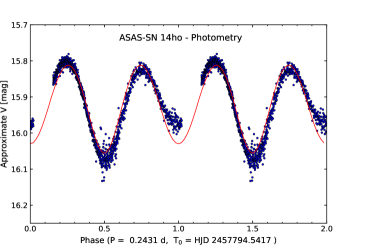
Figure 4: Differential magnitudes of ASASSN-14ho transformed to approximate $V$ plotted as a function of orbital phase, repeated once for clarity. The red curve shows a model of the ellipsoidal variation.

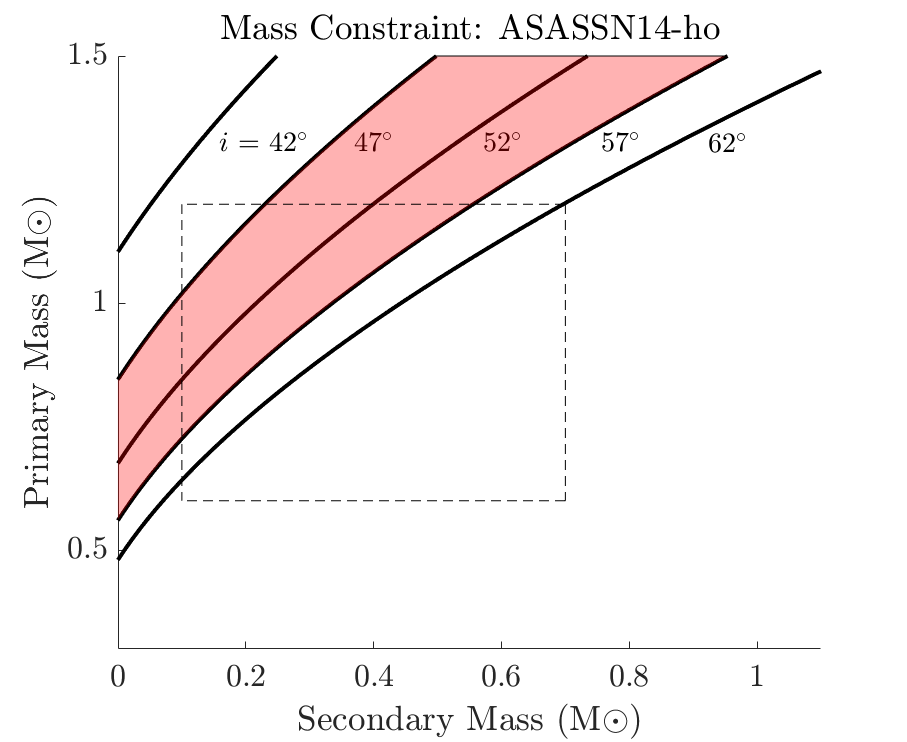
Figure 5: Constraining masses of ASASSN-14ho using mass function. The shaded area represents the inclination range we report as most reasonable based on the photometry modeling. The dotted box represents a reasonable range of masses for each component in the system.

4 V1062 Cyg Results

4.1 Period and Radial Velocities

The absorption line velocities in V1062 Cyg give an unambiguous $P_{\rm orb}=348.25\,\pm\,0.84$ min (note that the photometry discussed in 4.3 suggests a slightly shorter period). The emission-line velocities corroborate the period found in the absorption lines. The H$\alpha$ emission line showed a complex structure, with the wings and core of the line moving roughly in antiphase. To measure the line wing velocities we used a ‘gau2’ function separated by 32 Å, and for the core we used a ‘dgau’ optimized for 12 Å FWHM. Table 5 gives parameters of least-squares sinusoidal fits, and Figure 6 plots the velocities of the absorption lines and the two components of the H$\alpha$ line as a function of orbital phase, together with the best fits.

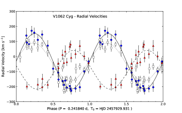
Figure 6: Radial velocities from V1062 Cyg folded on the adopted orbital period and repeated once for clarity, together with the best-fitting sinusoids at the adopted orbital period. The symbols are as follows: Blue circles and solid line; absorption-line velocities of the secondary star. Red triangles and dashed curve; H$\alpha$ emission line wings; open squares and dotted curve; H$\alpha$ emission line core.

Figure 7 shows a phase-resolved greyscale representation of the spectrum centered on the H$\alpha$ emission line. The velocity modulation of the bright line core is nearly in phase with the absorption, while the weaker, more diffuse wing component appears to move in antiphase. This suggests that the core emission arises from the secondary star, caused perhaps from irradiation of the side facing the white dwarf (Steeghs et al., 2001), or possibly from magnetic activity. The velocity modulation of the wings is apparently consistent with the accretion disk.

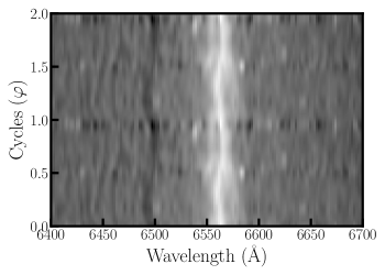
Figure 7: Single-trailed spectrum on V1062 Cyg, centered on the H$\alpha$ emission line.

4.2 Spectral Type

The spectral type of the secondary is near M0.5. The total and subtracted spectra of V1062 Cyg are presented together in Figure 8.

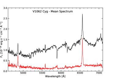
Figure 8: Average spectrum of V1062 Cyg; the lower trace (red) shows the spectrum after subraction of a scaled spectrum of Gliese 486 (type M0.5V).

4.3 Photometry and Stellar Parameters

Figure 9 shows the light curve, which displays double-peaked structure similar to ASSASN-14ho (Section 3.3). The ellipsoidal model does not fit as well as for ASASSN-14ho, but again clearly accounts for most of the variation. Much of the data between phases 0.25 and 0.6 were affected by an intermittent telescope control problem that grossly degraded the images. The light curve models give acceptable fits for $i=50\,\pm\,5^{\circ}$; the curve drawn is for $i=50$ degrees, $M_{1}=0.8\ {\rm M}_{\odot}$, $M_{2}=0.5\ {\rm M}_{\odot}$, and a secondary star with $T_{\rm eff}=3800$ kelvin and extra light equivalent to $3\times 10^{-17}$ erg cm^-2 s^-1 Å^-1. In Figure 10, we show the mass constraints for V1062 Cyg for a variety of potential inclinations.

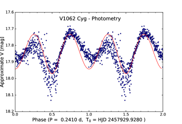
Figure 9: Differential magnitudes of V1062 Cyg transformed to approximate $V$ plotted as a function of orbital phase, repeated once for clarity. The red curve shows a model of the ellipsoidal variation.

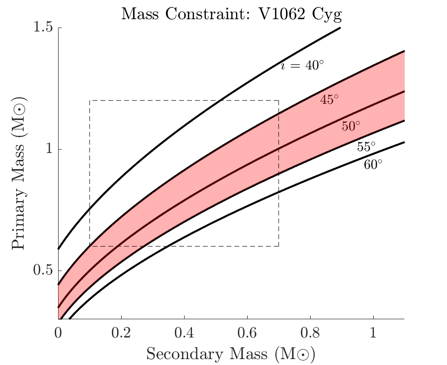
Figure 10: Mass constraints for V1062 Cyg. The shaded area indicates the inclination range we estimate from the light-curve model. The dotted box represents the reasonable range of masses for each component in the system.

5 Discussion

For ASASSN-14ho, we find the orbital period $P=350.14\,\pm\,0.15$ min and determine the secondary’s spectral type to be K4 $\pm$ 2 subclasses. By modeling the light curve, we estimate $i=52\,\pm\,5^{\circ}$. The mass function and inclination suggest white dwarf mass $M_{1}>0.8$ M_⊙.

For V1062 Cyg, we find $P=348.25\,\pm\,0.60$ min, and classify the secondary as M0.5. The light curve yielded $i=50\,\pm\,5^{\circ}$.

Both systems are dwarf novae with late-type secondary stars that dominate the optical flux. Both systems have orbital periods very close to 5.8 hr, well above the period gap of 2-3 hrs (Warner, 1995). The period gap is conventionally understood to represent a transition between two mass accretion stages in the CV’s lifetime (Howell et al., 2001).

Despite their nearly-identical orbital periods, the two systems’ secondary stars differ significantly in spectral type. Knigge et al. (2011) tabulate a semi-empirical sequence of the mean properties of CV secondaries, which gives $M_{2}=0.67{\rm M_{\odot}}$ and a spectral type of M0 for typical secondaries at this period. Our observations of V1062 Cyg are consistent with this, but the secondary of ASSASN-14ho is somewhat warmer and significantly less massive than their fiducial sequence. The empirical donor star data tabulated by Knigge (2006) does include secondaries as warm as that of ASASSN-14ho near this period.

The H$\alpha$ line profile of V1062 Cyg shows an unusual narrow component that moves in phase with the secondary star, as well as a fainter diffuse component that moves approximately with the white dwarf and accretion disk. This may arise from irradiation of one face of the secondary star. Very narrow H$\alpha$ lines phased with the secondary are sometimes seen in VY Scl stars during extreme low states (see e.g. Weil et al. 2018 and references therein). Far-ultraviolet observations might clarify whether the white dwarf or accretion structures in this system are unusually hot.

References

- Barwig & Schoembs (1983) Barwig, H., & Schoembs, R. 1983, A&A, 124, 287
- Bochkarev et al. (1979) Bochkarev, N. G., Karitskaia, E. A., & Shakura, N. I. 1979, Soviet Ast., 23, 16
- Claret et al. (2012) Claret, A., Hauschildt, P. H., & Witte, S. 2012, A&A, 546, A14
- Coppejans et al. (2013) Coppejans, R., Gulbis, A. A. S., Kotze, M. M., et al. 2013, PASP, 125, 976
- Crause et al. (2016) Crause, L. A., Carter, D., Daniels, A., et al. 2016, in Proc. SPIE, Vol. 9908, Society of Photo-Optical Instrumentation Engineers (SPIE) Conference Series, 990827
- Drake et al. (2009) Drake, A. J., Djorgovski, S. G., Mahabal, A., et al. 2009, ApJ, 696, 870
- Gaia Collaboration et al. (2016) Gaia Collaboration, Prusti, T., de Bruijne, J. H. J., et al. 2016, A&A, 595, A1
- Gaia Collaboration et al. (2018) Gaia Collaboration, Brown, A. G. A., Vallenari, A., et al. 2018, A&A, 616, A1
- Henden et al. (2015) Henden, A. A., Levine, S., Terrell, D., & Welch, D. L. 2015, in American Astronomical Society Meeting Abstracts #225, Vol. 225, 336.16
- Hoffmeister (1965) Hoffmeister, C. 1965, Information Bulletin on Variable Stars, 80
- Horne (1986) Horne, K. 1986, PASP, 98, 609
- Howell et al. (2001) Howell, S. B., Nelson, L. A., & Rappaport, S. 2001, ApJ, 550, 897
- Kepler et al. (2007) Kepler, S. O., Kleinman, S. J., Nitta, A., et al. 2007, MNRAS, 375, 1315
- Knigge (2006) Knigge, C. 2006, MNRAS, 373, 484
- Knigge et al. (2011) Knigge, C., Baraffe, I., & Patterson, J. 2011, ApJS, 194, 28
- North et al. (2002) North, R. C., Marsh, T. R., Kolb, U., Dhillon, V. S., & Moran, C. K. J. 2002, MNRAS, 337, 1215
- Prieto et al. (2014) Prieto, J. L., Sturch, L., Madore, B., et al. 2014, The Astronomer’s Telegram, 6619
- Ritter & Burkert (1986) Ritter, H., & Burkert, A. 1986, A&A, 158, 161
- Schneider & Young (1980) Schneider, D. P., & Young, P. 1980, ApJ, 238, 946
- Schreiber et al. (2016) Schreiber, M. R., Zorotovic, M., & Wijnen, T. P. G. 2016, MNRAS, 455, L16
- Steeghs et al. (2001) Steeghs, D., Marsh, T., Knigge, C., et al. 2001, ApJ, 562, L145
- Stetson (1987) Stetson, P. B. 1987, PASP, 99, 191
- Thorstensen (2013) Thorstensen, J. R. 2013, PASP, 125, 506
- Thorstensen et al. (2016) Thorstensen, J. R., Alper, E. H., & Weil, K. E. 2016, AJ, 152, 226
- Thorstensen & Armstrong (2005) Thorstensen, J. R., & Armstrong, E. 2005, AJ, 130, 759
- Tonry & Davis (1979) Tonry, J., & Davis, M. 1979, AJ, 84, 1511
- Warner (1995) Warner, B. 1995, Cambridge Astrophysics Series, 28
- Weil et al. (2018) Weil, K. E., Thorstensen, J. R., & Haberl, F. 2018, AJ, 156, 231