A model for phonetic changes driven by social interactions

Abstract

We propose a stochastic model to study phonetic changes as an evolutionary process driven by social interactions between two groups of individuals with different phonological systems. Particularly, we focus on the changes in the place of articulation, inspired by the drift //$\rightarrow$/h/ observed in some words of Latin root in the Castilian language. In the model, each agent is characterized by a variable of three states, representing the place of articulation used during speech production. In this frame, we propose stochastic rules of interactions among agents which lead to phonetic imitation and consequently to changes in the articulation place. Based on this, we mathematically formalize the model as a problem of population dynamics, derive the equations of evolution in the mean field approximation, and study the emergence of three non–trivial global states, which can be linked to the pattern of phonetic changes observed in the language of Castile and in other Romance languages.

I Introduction

Oral communication, as the process of transmitting concepts and ideas from one individual to another by word of mouth, has been a main feature of human kind since the first primitive societies. Historically, research in this field has been faced by anthropologists and linguistics. However, in the last years the interest for the development of new technologies related to automatic speech recognition, specially in artificial intelligent systems [1], has made it an active multidisciplinary area of research [2, 3, 4, 5].

Particularly, in the field of the physics of complex systems, the topic has been faced from the point of view of competition and evolution. In ref. [6], for instance, by performing agent based model simulations, Castelló et al. analyze the competition between two socially equivalent languages, and study the dynamics in structured populations in the frame of complex network theory. Similarly, in ref. [7], Stauffer et al. focus on the concepts of evolution, analyzing the rise and fall of languages using both macroscopic differential equations and microscopic Monte Carlo simulations. In ref. [8] likewise, Baronchelli et al. focus on the analysis of the emergence of grammatical constructions, reporting an order/disorder transition where the system goes through a sharp symmetry breaking process to reach a shared set of conventions. Moreover, the co-evolution of symbols and meanings has been studied through elementary language games by Puglisi et al. in ref. [9] showing the emergency of a hierarchical category structure.

In the frame of linguistic theories, on the other hand, speech production might be thought as the combination of several cognitive processes: the selection of the proper words to express an idea, the suitable choice of a grammatical form, and the production of sounds via the motor system and the vocal apparatus [10]. In this work we focus on the latter, therefore, in the following we describe the most relevant concepts regarding the production of sounds.

Formally, phonemes are the minimal units of either vocalic or consonant sounds needed to produce words. In this regard, the set of phonemes which encompasses all the sounds needed to produce every word in a given language, define a phonological system (PS). It is particularly important to emphasize that phonemes are not sounds but formal abstractions of speech sounds. Any phoneme in a PS might be a representation for a family of sounds, technically called phones which are recognized by speakers and linked to a specific sound during oral communications [11]. Physiologically, the process by which the vocal apparatus produces sounds is called phonation [12]. Through this mechanism, humans are able to produce a wide range of sounds, usually divided into two groups: vowels and consonants [13]. Let us focus on consonants production. In this case, the phonetic apparatus uses a combination of tongue, lips, teeth and the soft palate, in order to shape the different air obstructions needed to produce the sounds. The point inside the vocal cavity where the obstruction occurs is called articulation place (AP), and the manner in which the obstruction is shaped is called articulation mode (AM). This two dimensions, AP and AM, are commonly used to categorize the main features of the consonants in a particular PS.

Since languages are in continuous evolution, it is well known that under certain conditions, this process might lead to changes into the PS [14]. Particularly, in this work we are interested in studying phonetic changes in consonants related to variations in the AP. In this regard, it has been observed that these changes are enhanced when two or more groups of people with different languages are forced to socially interact [15, 16, 17, 18, 19]. For instance, when a group invades other group’s territory, or when two groups establish economic relations (trade, exchange of services, etc). The linguistic, phonetic and grammatical mutual influences produced by the interaction among the groups, define a linguistic stratum (LS) [20, 21], where the persistent social interaction over time, in a process of oral communication, guides the evolution to a common PS and to a common new language.

A notable example of phonetic change in the AP due to a LS, and the main inspiration of this work, is the case of the glottalization of the bilabial fricative phoneme // towards the glottal fricative /h/ (hereafter referred to as the change //$\rightarrow$/h/), and its subsequent disonorisation in some Latin root words of Castilian language (see table 1). It is thought that the social process which led to the LS in this particular case, was related to the social interactions among the prehispanic tribes (Iberics, Asturians, and mainly Vascons) and the Romans, which were forced to socially interact in the Iberian peninsula—during the period of Rome’s domain—from the second to the ninth cenrury, AD [22, 23, 24]. In this particular LS there were groups of people with a PS (based on Celtic language), socially interacting with other group of people with a total different PS (based on Latin language).

In this context, it is thought that the change //$\rightarrow$/h/ is related to prehispanic tribes speakers performing changes in the AP during fricative production, trying to improve their communication skills with Latin speakers [25]. Notably, these changes are not observed in other Romance languages on the Iberian peninsula, as the case of Portuguese or Catalan, which emerge from a similar LS than Castilian. This fact led to researchers to theorize about the properties of this particular LS, and additionally to propose alternative theories [26, 27]. Until now, it seems there is not a total consensus regarding the causes which led to these different evolutions of the Romance languages, therefore the case is currently considered by linguistics as an open problem.

Motivated on the historical observations regarding the changes //$\rightarrow$/h/, the aim of this work is to propose a model of language competition [28, 29, 30, 31, 32] which captures the internal dynamics of a LS. The model consider two social groups having different PS, where the changes in the articulation places are guided by social interactions based on rules of phonetic imitation.

We face the problem in the frame of population dynamics, where we study the evolution of the changes in both groups, and the emergence of general states of pronunciation in the LS.

This paper is divided into three main sections: in section II we mathematically formalize the model, define the main variables, propose the rules of the interactions and describe the dynamics; in section III we derive from first principles the equations of evolution; and, lastly, in section IV we analyze the emergence of global states by performing an analysis of both the evolution equations and agent based model simulations. We found that by tuning the parameters related to the social interactions in the LS, our model shows the emergence of three general global states which capture qualitatively the observations of the emergent Romance languages of the Iberian peninsula, reinforcing from our mathematical approach, the stratum-based theories present in the literature.

II The model

We aim to model a process of phonetic imitation which leads to changes in the AP during consonant production. Accordingly, we have made the following simplifications: we will (i) limit our analysis to the changes in the AP, neglecting any change in the AM; (ii) propose there are only three possible AP in the vocal cavity, a front place (bilabial, labio-dental), a middle place (dental, alveolar and post-alveolar) and a back place (palatal, velar, uvular and glottal); (iii) suppose there are two PS in the LS, one which favors front and middle production, and other which favor middle and back; and (iv) study the evolution of the changes in the pronunciation of a single word.

In this frame, we define the main elements of the model as follows:

• $A,B$ are two groups of agents in a stratum $LS$;

• $N_{A}$, $N_{B}$ are the number of agents in $A,B$ and $N=N_{A}+N_{B}$ the total number of agents in $LS$;

• $S$ is the state of an agent in the $LS$ at time $t$, where $S\in\{1,2,3\}$ represents the AP of agent $i$, such that: $1=front$, $2=middle$, $3=back$;

• $PS^{A},PS^{B}$ are the phonological systems of $A,B$, indicating that $A$ has $S=1,2$ as preferential states (front– middle); and conversely, $B$ has $S=2,3$ (middle– back).

Latin	Castilian	Portuguese	English Translation
facere	hacer	fazer	to do/ to make
femina	hembra	fêmea	female
ferru	hierro	ferro	iron
filiu	hijo	filho	son
folia	hoja	folha	leaf
fumu	humo	fumaça	smoke

Table 1: Some examples of Latin root words which show the change //$\rightarrow$/h/ in Castilian (column 1). In column 2, we show the translation into Portuguese in order to show the change in this case did not happen. In column 3, we show the translation into English as a reference. In order to clarify, note that in column 1, the phonetic transcription of letter f is the bilabial phoneme //, and in column 2, the phonetic transcription of letter h is the glottal phoneme /h/.

In the evolutionary process, at time $t$, we randomly take from the set $A\cup B$ an active agent and a reference agent. The state of the former will change according to the state of the latter, guided by the following imitation rules which we summarize by using the usual chemical reactions notation,

where $A_{i}$ and $B_{i}$ are agents of group A and B, respectively, in state $S=i$. For example, Eq. (1) states that a member of the population $A_{2}$ can interact with a member of $A_{3}$ and that the result of the interaction are two members of the population $A_{2}$.

The rules ($1a-1d$) are introduced in order to emulate a process of imitation, where interactions between agents of different groups lead to non preferential states of pronunciation, and interactions between agents of the same group, conversely, reinforce the preferential states of the group. In this respect, probabilities $q,p$ define the interaction strength between agents of different groups, and the interaction strength between agent of the same group, respectively. Moreover, the noisy component expressed by rules $(1e)$ and $(1f)$, captures the variations caused by both random phonetic changes and the production of possible allophones in both $PS^{A}$ and $PS^{B}$, respectively. On the other hand, note that in the frame of the proposed imitation rules, the changes in the states occur only when the AP distance, between the referent and the active agents is equal to one (i.e. $|\Delta S_{ij}|=1$, with $i,j$ reference and active agents). The idea here is modeling the changes in the context of close or similar sounds [33, 34, 35] between the different PSs, neglecting the contribution to the changes of any other possible interactions.

In this theoretical frame, our proposal has been inspired in the models of opinion formation dynamics [36, 37] where social interactions, in the context of a social debate, drives the population to emergent states of consensus or polarization [38, 39, 40].

Macroscopically, in the frame of evolutionary dynamics, the global state of the system can be analyzed by counting the number of agents in $A,B$, in the states $S=1,2,3$. In the following section, based on this idea we introduce the master equation of the process and derive the evolution equations for the first moments, or mean-field approximation.

III The equations of evolution

Let $N^{A}_{i}$, $N^{B}_{i}$ be the number of agents in $A,B$ in state $S=i$, with $i=1,2,3$ (hereafter referred to as the occupation numbers). The master equation of the system is given by,

$$\frac{\partial P(\vec{x};t)}{\partial t}=\sum_{\vec{y}\neq\vec{x}}T(\vec{x}|\vec{y})P(\vec{y};t)-\sum_{\vec{x}\neq\vec{y}}T(\vec{y}|\vec{x})P(\vec{x};t),$$ (1b)

where $\vec{x}=(N^{A}_{1},N^{A}_{2},N^{A}_{3};N^{B}_{1},N^{B}_{2},N^{B}_{3})$ is the so called occupation vector; $P(\vec{x};t)$ is the probability to find the system with an occupation vector $\vec{x}$ at time $t$, and $T(\vec{x}|\vec{y})$ is a transition probability from a global state given by an occupation vector $\vec{y}$ to another given by $\vec{x}$. In this approach, we are considering a fixed population in both groups, therefore for all $t$ we have,

$$\begin{split}N_{A}&=N^{A}_{1}+N^{A}_{2}+N^{A}_{3},\\ N_{B}&=N^{B}_{1}+N^{B}_{2}+N^{B}_{3},\\ N&=N_{A}+N_{B}.\end{split}$$ (1c)

From the master equation (1b), we can derive the evolutionary equations for the first moment of the occupation numbers (mean-field approximation). For instance, for $N^{A}_{2}$ we have,

$$\frac{d}{dt}\left\langle N^{A}_{2}\right\rangle=\left\langle T(N^{A}_{2}+1|N^{A}_{2})\right\rangle-\left\langle T(N^{A}_{2}-1|N^{A}_{2})\right\rangle,$$ (1d)

the transitions $T$ are defined by the rules proposed in the last section, and depend on probabilities $p$, $q$, and $r$. For the case by which the system increases one agent in $N^{A}_{2}$, $T$ can be written as

$$T(N^{A}_{2}+1|N^{A}_{2})=\frac{N^{A}_{1}}{N}r+\frac{N^{A}_{3}}{N}\frac{N^{A}_{2}}{N-1}p,$$ (1e)

where the first term is the probability of finding an agent of group A in state $1$, times the probability it randomly goes to state $2$; and the second term is the probability of one interaction between an active agent of group $A$ in state $3$ and a reference agent of the same group in state $2$, leads to the former to imitate the latter with probability $p$.

For the case in which the occupation number $N^{A}_{2}$ decrease in one agent, the transition is given by,

$$T(N^{A}_{2}-1|N^{A}_{2})=\frac{N^{A}_{2}}{N}\frac{N^{B}_{3}}{N-1}q+\frac{N^{A}_{2}}{N}r,$$ (1f)

where the first term shows the loss of an active agent of group A in state $2$ due to the interaction with a reference agent of group B in state $3$, and the second term stands for the random loss of an agent in $2$ who moves to $1$.

Replacing 1e and 1f in equation (1d), we obtain,

$$\begin{split}\frac{d}{dt}\left\langle N^{A}_{2}\right\rangle&=\left\langle\frac{N^{A}_{1}}{N}r+\frac{N^{A}_{3}}{N}\frac{N^{A}_{2}}{N-1}p\right\rangle-\\ &-\left\langle\frac{N^{A}_{2}}{N}\frac{N^{B}_{3}}{N-1}q+\frac{N^{A}_{2}}{N}r\right\rangle,\\ \\ \frac{d}{dt}\left\langle N^{A}_{2}\right\rangle&=\frac{r}{N}\left\langle N^{A}_{1}\right\rangle+\frac{p}{N(N-1)}\left\langle N^{A}_{3}N^{A}_{2}\right\rangle-\\ &-\frac{q}{N(N-1)}\left\langle N^{A}_{2}N^{B}_{3}\right\rangle-\frac{r}{N}\left\langle N^{A}_{2}\right\rangle.\end{split}$$ (1g)

From now on, we will consider the evolution of the numbers are uncorrelated, then $\left\langle N^{A}_{2}N^{B}_{3}\right\rangle=\left\langle N^{A}_{2}\right\rangle\left\langle N^{B}_{3}\right\rangle$ and $\left\langle N^{A}_{3}N^{A}_{2}\right\rangle=\left\langle N^{A}_{3}\right\rangle\left\langle N^{A}_{2}\right\rangle$.

Moreover, we re–scale the time as $t\rightarrow\frac{t}{N}$, use the approximation for large population $(N-1)\approx N$, and define the occupation number as fractions of the total population: $a_{1}=\left\langle\frac{N^{A}_{1}}{N}\right\rangle$, $a_{2}=\left\langle\frac{N^{A}_{2}}{N}\right\rangle$, $a_{3}=\left\langle\frac{N^{A}_{3}}{N}\right\rangle$, $b_{3}=\left\langle\frac{N^{B}_{3}}{N}\right\rangle$. Using the notation and approximations introduced above, we can write equation (1g) as follows,

$$\dot{a_{2}}=ra_{1}+pa_{2}a_{3}-qa_{2}b_{3}-ra_{2}$$ (1h)

Similarly, it is possible to obtain the equations for the evolution of the other occupation numbers, which define the following system of coupled differential equations,

$$\begin{split}\dot{a_{1}}&=r(a_{2}-a_{1})\\ \dot{a_{2}}&=-r(a_{2}-a_{1})+pa_{2}a_{3}-qa_{2}b_{3}\\ \dot{a_{3}}&=-pa_{2}a_{3}+qa_{2}b_{3}\\ \dot{b_{1}}&=-pb_{1}b_{2}+qb_{2}a_{1}\\ \dot{b_{2}}&=pb_{1}b_{2}-qb_{2}a_{1}-r(b_{2}-b_{3})\\ \dot{b_{3}}&=r(b_{2}-b_{3})\end{split}$$ (1i)

It is important to highlight that since we are now working with the fractions of the occupation numbers, the constraints related to the fixed population become: $n_{A}=a_{1}+a_{2}+a_{3}$, $n_{B}=b_{1}+b_{2}+b_{3}$, and $n_{A}+n_{B}=1$, where $n_{A}=\frac{N_{A}}{N}$, $n_{B}=\frac{N_{B}}{N}$. The constraints also show that it is possible to reduce the rank of the system to four, however, for the sake of clarity, we decided to keep the six equations for a more detailed analysis.

Lastly, note that, if there are equilibrium points in system (1i), in the frame of our model, these may be related to the population reaching consensus about a common general way of pronunciation in both groups. In the following section we will probe the existence of four equilibrium points, and will show that the stability of these emergent states strongly depends on the interactions rates intra- and inter-group.

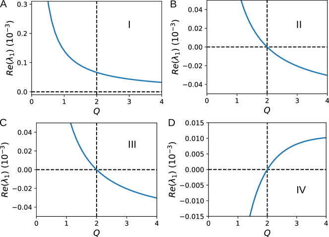
Figure 1: Stability analysis. Real part of the largest non-trivial eigenvalue of the Jacobian Matrix ($\lambda_{1}$), as a function of the parameter $Q$. Panels A,B,C and D show the numerical calculation for the equilibria I, II, III and IV, respectively. Note that when $Re(\lambda_{1})>0$ the system is unstable, therefore equilibrium I will be unstable for all value of $Q$; II and III will be unstable for $Q<2$, and IV for $Q>2$.

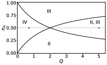
Figure 2: Projection of the phase diagram in the plane $(n_{A},Q)$. The curves $n_{A}=2/(2+Q)$ and $n_{A}=Q/(2+Q)$ divide the plane into four regions with different stability. The labels for each region correspond to the equilibria that are stable inside the region. The two blue markers represent the parameters that were used in the main text.

IV The emergent states

At time $t\rightarrow\infty$, if an equilibrium exists, it must satisfy $\dot{a_{i}}=0$ and $\dot{b_{i}}=0$. In these conditions, from Eqs. (1i) and using the population constraints, it is possible to probe the existence of four non trivial equilibrium points,

1. $\vec{n}_{eq}=(0,0,n_{A};n_{B},0,0)$

2. $\vec{n}_{eq}=(0,0,n_{A};0,\frac{n_{B}}{2},\frac{n_{B}}{2})$

3. $\vec{n}_{eq}=(\frac{n_{A}}{2},\frac{n_{A}}{2},0;n_{B},0,0)$

4. $\vec{n}_{eq}=(\alpha,\alpha,Q\beta;Q\alpha,\beta,\beta)$, where $\alpha=\frac{2n_{A}-Qn_{B}}{4-Q^{2}}$,

$\beta=\frac{2n_{B}-Qn_{A}}{4-Q^{2}}$ and $Q=\frac{q}{p}$.

The first equilibrium can only be reached if the initial conditions are set at this point, later we will show this equilibrium is unstable. Equilibria II and III are the cases where the system loses the back and the frontal AP, respectively. Equilibrium IV, on the other hand, shows a mixed final state, where the system reaches a balance among the three states of pronunciation.

The stability analysis around the equilibrium can be performed by analysing the eigenvalues of system (1i) (see Appendix A).

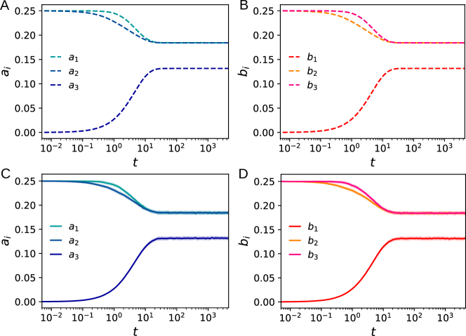
Figure 3: The case of equilibrium IV stable. For $Q=0.7$, panels A and B show the first moment evolution of the numbers related to group A ($a_{1},a_{2},a_{3}$) and B ($b_{1},b_{2},b_{3}$), respectively. The curves are the outcome of the evolution of Eqs. (1i), which were solved by performing a Runge Kutta 8th order method. Panels C and D show the average curves over $100$ realizations, of the numbers in the ABM. The shadow indicate the standard deviation around the mean value. In these conditions, the population evolves to equilibrium IV, a mixed state of pronunciation where the system reaches $\vec{n}_{eq}=(\frac{5}{27},\frac{5}{27},\frac{7}{54};\frac{7}{54},\frac{5}{27},\frac{5}{27})\approx(0.18,0.18,0.13;0.13,0.18,0.18)$.

We are particularly interested in studying the evolution of the system as a function of $Q$ since this parameter controls the interaction between $A$ and $B$, and also rules the population state of the equilibrium point IV. To this purpose, we set a constant equal population $n_{A}=n_{B}$, $r=0.5$, $q=0.5$ and vary the parameter $p$, in order to focus only in the study of the effect of $Q=q/p$, on the equilibrium conditions of the system. In this frame, we have calculated the eigenvalues as a function of $Q$, and studied the sign of the real part of the eigenvalues to evaluate the stability conditions.

The plots in figure 1 show the curves for the real part of the largest non–trivial eigenvalue, $Re(\lambda_{1})$ vs. $Q$ for the four equilibrium points. Panel A in this figure shows the calculation for state I. We can see that for all $Q$ there is an eigenvalue with positive real part, which means this equilibrium state is always unstable. In panels B and C we can observe that states II and III behave similarly each other. This is expected because these two states are symmetric. States II and III are unstable for $Q<2$ since they have at least one eigenvalue with positive real part. Finally, panel D shows the calculation for equilibrium state IV; in this case, complementary to states II and III, the equilibrium is unstable for $Q>2$.

Clearly, coefficient $Q$, which measure the relative intra- and inter-groups imitation rates, determines the stability of the different equilibrium states of the system. We can understand this phenomenon by reasoning as follows: At $Q=2$, the inter-group interactions equals the sum of the interaction rates within each group ($Q=2\rightarrow q=p+p$), and equilibrium IV becomes $\vec{n}_{eq}=(\alpha,\alpha,Q\beta;Q\alpha,\beta,\beta)=(\frac{1}{8},\frac{1}{8},\frac{1}{4};\frac{1}{4},\frac{1}{8},\frac{1}{8})$, i.e. there is a balance between the number of agents in preferential and non-preferential states of pronunciation in both groups ($n^{A}_{1}+n^{A}_{2}=n^{A}_{3}$ and $n^{B}_{1}=n^{B}_{2}+n^{B}_{3}$). For $Q>2$, the system loses the balance, the number of agents in non– preferential states becomes larger than the number of agents in preferential states, hence equilibrium IV becomes unstable and depending on the initial conditions the system evolves to equilibrium II or III. Furthermore, in the stochastic version of the model and balanced initial conditions fluctuations can determine the final equilibrium state, which occurs with equal probability for states II and III.

Finally, a more general stability analysis of the mean field model, which includes unbalanced conditions $n_{A}\neq n_{B}$, is conducted in Appendix A. The main results of this analysis is summarized in the phase diagram shown in Fig. 2. There are four stability regions in the $n_{A}$ - $Q$ plane. One for point IV at low values of Q. Another two for points II and III, respectively, and one region where point II and III coexist. All our analysis will be restricted to two representative values of $Q$ in this phase diagram.

In order to visualize the time evolution of the occupation number in the system, and to study the convergence to the equilibrium points, we solved numerically the set of coupled differential equations given in Eqs. (1i), and also performed numerical simulations of the stochastic agent based model (ABM)—using the rules proposed in section II—in order to test the effect of fluctuations in the dynamics of the system. In a first approach we explore two limit cases far for the singular point $Q=2$: the case of $Q=0.7$ where the inter–group interaction domain the dynamics, and the case of $Q=5$ where, conversely, the dynamic is governed by the intra–group interactions. For this purpose, we set (i) the initial conditions on $\vec{n}(t=0)=(\frac{n_{A}}{2},\frac{n_{A}}{2},0;0,\frac{n_{B}}{2},\frac{n_{B}}{2})$ (preferential states for both groups), (ii) the fraction of agents such that $n_{A}=n_{B}$ (equal population in both group), (iii) the parameters $r=0.5$ and $q=0.5$, and (iv) for the ABM simulations, a population size of $N=10^{4}$. The results are summarized in the plots of figure 3 and 4, which we describe in the following. Figure 3 shows the evolution of the occupation numbers for $Q=0.7$ where state IV is stable. Panels A and B show the evolution in the mean field approximation (Eqs. (1i)), whereas panels C and D show the outcome of the ABM; here we have averaged the results over $100$ performed simulations. We can see that, as expected, the system evolves toward equilibrium IV and the mean reaches the value $\vec{n}_{eq}=(\alpha,\alpha,Q\beta;Q\alpha,\beta,\beta)=(\frac{5}{27},\frac{5}{27},\frac{7}{54};\frac{7}{54},\frac{5}{27},\frac{5}{27})$.

Figure 4, by contrast, shows the evolution for $Q=5$ where equilibria II and III are stable; in this case, the realization showed in the plots went to equilibrium II. Notably, at the beginning of the evolution, the system seems to stabilize at equilibrium IV, but at larger times moves toward equilibrium II, as expected. The arrows in figure 4 panel A, indicate the relaxation times operating at each regime, given by the inverse of the eigenvalues ($\propto 1/\lambda_{i})$.

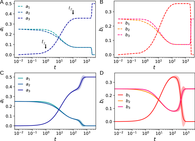
Figure 4: The case of equilibrium II stable. For $Q=5$, panels A and B show the first moment evolution of the numbers related to group A and B, respectively. Panels C and D, on the other hand, show the average curves over 100 realizations, of the numbers in the ABM. The shadow in the plots indicate the standard deviation whch we see it increases when the system reach the unstable equilibrium IV. Note how at the beginning the system seems to evolve toward IV, but escape toward the equilibrium II, which is stable in these conditions ($\vec{n_{eq}}=(0,0,\frac{1}{2};0,\frac{1}{4},\frac{1}{4})$). The arrows in panel A, indicate the time scales obtained from the eigenvalues analysis: $t_{1}\approx 1$ and $t_{2}\approx 10^{2}$.

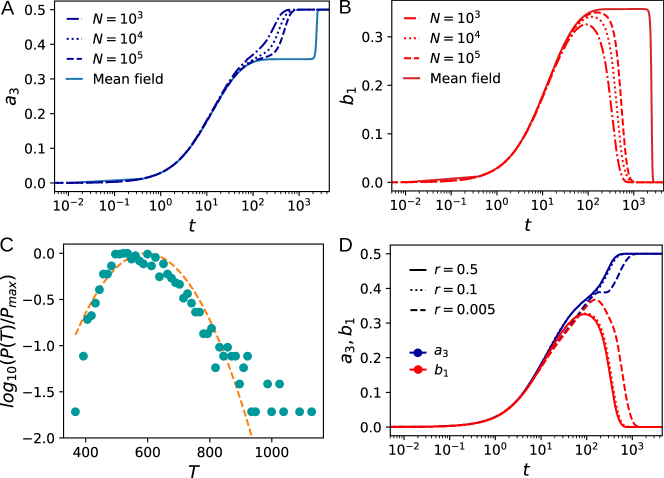
Figure 5: Panel A and B, the average curves for the evolution of the numbers $a_{3}$ and $b_{1}$, respectively, for different values of the population size $N$, compared with the mean field approximation in order to see the finite size effect. Panel C, distribution of final times $T$, needed to the system reach equilibrium II at $Q=5$. The dashed line in the background indicate a Gaussian distribution with the same mean and standard deviation, which helps to visualize the presence of a large tail in distribution $P(T)$. Panel D, the average curves for the evolution of the numbers $a_{3}$ and $b_{1}$ for different values of the parameter $r$.

In a second approach, we explore finite size effects in the system, by performing ABM simulation for different sizes ($N$) of the total population and comparing with the mean field approximation. For the case $Q=5$, we can see from figure 5 panels A and B, that the finite size effects become notable once the system reaches the unstable equilibrium IV. The larger the population the lower the fluctuations, therefore the system will spend more time at the unstable equilibrium IV before fluctuations lead it to the stable state II.

In connection with the expressed above, we measured the distribution of times ($T$) needed for the system to reach the final equilibrium at $Q=5$ by performing $2000$ realizations of the stochastic model. Figure 5 panel C, shows the distribution obtained. We can see a non symmetric distribution with a peak around $T\approx 600$, and a tail at the right of the distribution. As we said before, in every realization the system stays in the unstable equilibrium IV before it reaches the final stable state, therefore the total time $T$ depends on the magnitude of the fluctuations which drive the system from the unstable equilibrium to the stable one. The latter explains the tail at the right of the distribution and also the differences in the final times observed among the stochastic simulations and the mean field approach.

On the other hand, as we show above the equilibrium points are not dependent of parameter $r$; however, since $r$ is a stochastic parameter of the model, the dynamics towards the equilibrium should depend on it. In Panel D on figure 5 we show the evolution of the numbers $a_{3}$ and $b_{1}$ for $r=0.5,\ 0.1,\ 0.005$. For the lowest value explored ($r=0.005$), we can see a different behaviour around the unstable equilibrium IV, which seems to indicate a link between the reduction of the stable attractor force and the reduction of $r$.

Lastly, in order to complete a global analysis, we test the system behaviour under changes in the initial conditions. Figure 6 panel A shows trajectories in the plane $a_{1}-a_{3}$ for $Q=5$, obtained from the mean field approach simulations, where we have tried different initial conditions for the numbers $a_{i}$, keeping $r=0.5$ (the different trajectories in the plane are indicating in the plot as $l_{i}$, $i=1,2,3,4$). We can see that depending on the proximity to the stable attractor II the system will explore the unstable equilibrium IV, as in the case of trajectories $l_{1}$, $l_{2}$ and $l_{4}$, or it will not as in the case of trajectory $l_{3}$. For the case of $l_{1}$ we have additionally plotted the trajectory obtained from a single stochastic realization.

The plot in figure 6 panel B, on the other hand, complements the information given in figure 5 panel D, showing the effect of parameter $r$ on the trajectories in the plane $a_{1}-a_{3}$. In this regards, the parameter $r$ regulates the velocity of the transitions $\ce{A_{1}<=>A_{2}}$ (and also $\ce{B_{2}<=>B_{3}}$). When $r$ is strong enough, these transitions occur much faster than the rest and thus, populations $A_{1}$ and $A_{2}$ tend to have the same number of individuals, independently on the initial conditions. This aspect explains why all the trajectories in Figure 6 panel A rapidly approximate to the line $a_{3}=-2a_{1}$. If the system starts from an initial condition with a low value of $a_{3}$, then the trajectory will be forced to go through equilibrium IV, as it can be seen in the figure. When we reduce the value of $r$, it is harder for the system to equal the values of $a_{1}$ and $a_{2}$ and thus, the trajectories in general deviate from the line and equilibrium IV is avoided, as we show in Figure 6 panel B.

In the frame of the proposed model, state II can be related to the change //$\rightarrow$/h/ in Castilian, and state III to the observed in other Romance languages like Portuguese or Catalan. Therefore, for $Q>2$, the model seems to capture very well the current pronunciations that emerged—from the real LS—in the Iberian peninsula. On the other hand, equilibrium IV, describes an emergent state of mixed pronunciation, which means there are agents using different AP to pronounce the same word. This is rarely observed in the real case, but can be used to understand the existence of some regionalism or local accents in the peninsula [41].

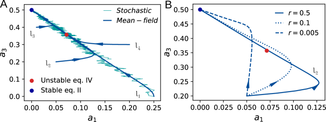
Figure 6: Trajectories in the plane $a_{1}-a_{3}$. Panel A, changing the initial conditions, keeping $r=0.5$. Panel B, changing parameter $r$, for trajectory starting from the same initial condition than $l_{2}$ in panel A. The blue lines correspond to the solution of the differential equations, while the cyan curve in Panel A corresponds to a single realization of the stochastic simulation, starting from the initial condition of trajectory $l_{2}$.

V Conclusions

In this work, we have proposed a model to study phonetic changes in the AP used for pronounce a single word as an evolutionary process guided by social interaction of imitation between two groups of people with different phonological systems. Inspired by the case of the change //$\rightarrow$/h/ in Castilian language, we have studied a fixed population made up of two groups of interacting people, A and B, such that group A has a trend to produce frontal fricatives and conversely group B has a trend to produce back fricatives. The rules of the model were proposed based on empirical observations, and were thought to link the phonetic changes with a process of social interactions inter- and intra-group. The model was mathematically formalized in section II as a stochastic process where the variable $S\in\{1,2,3\}$, representing the AP for every agent in the population, changes according to the proposed interaction rules.

In this frame we studied the temporal evolution of the occupation numbers, and from first principles, we derived the coupled system of differential equations which defines the dynamics in the mean field approximation. In the equilibrium, we found three non trivial final states, which we have related to the emergence of general states of consensus in the way a word is pronounced. In this regards, we found that when the rate of interaction among agents from different groups becomes larger than the sum of the rates within each group ($q>2p$), the system exhibits two emergent states (equilibria II and III) which capture very well both, the middle-back pronunciation used in Castilian and the front-middle pronunciation observed in other Romance languages, as the case of Portuguese. From a social point of view, we can link the condition $q>2p$ to the situation where the relation among individuals from different groups is larger enough to allow a common general consensus in spite of the cultural differences.

The model we have introduced is based on a mean field approach since all agents interact among them, hence it does not consider the influence of the structure of social interactions in reaching a consensus for the phonetic changes. This is of course a simplification, as it is known that the structure of social interactions strongly influences human behavior and the evolution of social and cognitive processes [42]. Even more, human mental lexicon is supposes to be assembled according to a multiplex network structure [43]. Hence, one can expect the network structure to play a key role in any particular dynamics of phonetic changes. However, Baxter, et al. [32] proved that in several neutral interactor models inspired in Trudgill’s theory for the emergence of New Zealand English, the structure of the underliying social network has a minor effect in the final state distribution of speaker’s grammar (linguemes) produced by these models. According to Trughill’s deterministic theory, frequency of use and accomodation are the only factors to be taken into account for the prevalence of a given lingueme. Our model is deterministic in terms of its parameters. The final phonetic state is correlated to the initial frequency of agents using a given phonetic system for the case $Q>2$ (states II and III), in those states one phonetic system prevails over the other. However, the proposed imitation mechanism that rules the interaction between agents of different phonetic systems, can lead to a final state in which the two phonetic systems coexist. This is particularly relevant in the analysis of Castilian phonetic when the system is considered as a whole. In this case the LS contains fricative words that keep the Latin pronunciation as well as other words that change to glottalization, which means that there is a coexistence of the articulation places in the global system.

Finally, more realistic models must consider the structures of social interactions in the dynamics. Then, it would be interesting to analyze the interplay between the network topology and the dynamics of phonetic changes generated by our model. In this regards, we let as an open problem to be faced in future works the study of the effect of the structure of social interactions in phonetic changes.

Appendix A Stability analysis

In this appendix we perform a stability analysis to extend the discussed in section IV.

Equation system (1i) can be reduced to a four-dimensional system using the constraints $a_{1}+a_{2}+a_{3}=n_{A}$ and $b_{1}+b_{2}+b_{3}=n_{B}$. Defining the parameters $\omega=r/p$, $Q=q/p$ and scaling the time as $\tau=pt$, we have

$$\begin{split}\dot{a_{1}}&=\omega(n_{A}-2a_{1}-a_{3})\\ \dot{a_{3}}&=(Qb_{3}-a_{3})(n_{A}-a_{1}-a_{3})\\ \dot{b_{1}}&=(Qa_{1}-b_{1})(n_{B}-b_{3}-b_{1})\\ \dot{b_{3}}&=\omega(n_{B}-2b_{3}-b_{1})\end{split}$$ (1j)

where we have changed the notation $\dot{x}\equiv dx/d\tau=(1/p)dx/dt$.

The Jacobian of the reduced system is

$$J=\begin{pmatrix}-2\omega&-\omega&0&0\\ a_{3}-b_{3}Q&a_{1}+2a_{3}-n_{A}-b_{3}Q&0&(n_{A}-a_{1}-a_{3})Q\\ (n_{B}-b_{3}-b_{1})Q&0&b_{3}+2b_{1}-n_{B}-a_{1}Q&b_{1}-a_{1}Q\\ 0&0&-\omega&-2\omega\end{pmatrix}.$$ (1k)

We proceed now to analyze the stability of each equilibrium. Before we start, it is important to notice that, as we have re-scaled the time as $\tau=pt$, the eigenvalues of the original system can be expressed as $\lambda=p\mu$, where $\mu$ are the eigenvales of the reduced system.

Evaluating 1k at equilibrium I and computing its eigenvalues, we have

$$\mu^{B}_{\pm} =\dfrac{n_{B}-2\omega\pm\sqrt{(n_{B}-2\omega)^{2}+4n_{B}\omega}}{2},$$ (1l)

$$\mu^{A}_{\pm} =\dfrac{n_{A}-2\omega\pm\sqrt{(n_{A}-2\omega)^{2}+4n_{A}\omega}}{2}.$$

The four eigenvalues are always real, and two of them (the ones with the plus sign) are always positive. This means that equilibrium I is always unstable, and thus, it lacks of physical interest.

For equilibrium II, the corresponding eigenvalues are

$$\mu_{\pm} =\dfrac{2n_{A}-Qn_{B}-4\omega\pm\sqrt{(2n_{A}-Qn_{B})^{2}+16\omega^{2}}}{4},$$

$$\mu_{3} =-\dfrac{n_{B}}{2},$$ (1m)

$$\mu_{4} =-2\omega.$$

The eigenvalues $\mu_{-}$, $\mu_{3}$ and $\mu_{4}$ are always negative, but $\mu_{+}$ can be either positive or negative. The region of the parameter space where it is negative (and thus, where the equilibrium is stable) is given by

$$Q>\dfrac{2n_{A}}{n_{B}}$$ (1n)

Considering $n_{B}=1-n_{A}$, the previous inequality can be solved for $n_{A}$ as

$$n_{A}<\dfrac{Q}{2+Q}.$$ (1o)

Equilibrium III is symmetric with respect to equilibrium II and its eigenvalues are

$$\mu_{\pm} =\dfrac{2n_{B}-Qn_{A}-4\omega\pm\sqrt{(2n_{B}-Qn_{A})^{2}+16\omega^{2}}}{4},$$

$$\mu_{3} =-\dfrac{n_{A}}{2},$$ (1p)

$$\mu_{4} =-2\omega.$$

Thus, the equilibrium is stable when

$$Q>\dfrac{2n_{B}}{n_{A}},$$ (1q)

which can be also expressed as

$$n_{A}>\dfrac{2}{2+Q}.$$ (1r)

Equilibrium IV exists only if $\alpha$ and $\beta$ are simultaneously greater than zero. It can be shown that the condition for this to happen is

$$\left(n_{A}-\dfrac{2}{2+Q}\right)\left(n_{A}-\dfrac{Q}{2+Q}\right)<0.$$ (1s)

To analyze the stability, lets first consider the particular case $n_{A}=n_{B}$. In this case, the corresponding eigenvalues are

$$\mu_{1,\pm}= \dfrac{-\left[n_{A}+2\omega(2+Q)\right]}{2(2+Q)}$$

$$\pm\dfrac{\sqrt{\left[n_{A}+2\omega(2+Q)\right]^{2}-4\omega n_{A}(4-Q^{2})}}{2(2+Q)},$$ (1t)

$$\mu_{2,\pm} =\dfrac{-\left[n_{A}+2\omega(2+Q)\right]}{2(2+Q)}$$

$$\pm\dfrac{\sqrt{\left[n_{A}+2\omega(2+Q)\right]^{2}-4\omega n_{A}(2+Q)^{2}}}{2(2+Q)}.$$

From these eigenvalues, $\mu_{1,\pm}$ and $\mu_{1,-}$ are always negative while $\mu_{1,+}$ is negative if and only if $Q<2$. For the general case $n_{A}\neq n_{B}$, we could not get explicit expressions for the stability analysis of this equilibrium. Instead, we performed simulations starting from different combinations of parameters and we found that, as long as condition 1s is satisfied, equilibrium IV is stable for $Q<2$ and unstable for $Q>2$.

Using Eqs 1o, 1r and 1s, and taking into account the discussion in the previous paragraph, we can draw a phase diagram for our model in the plane $(n_{A},Q)$, as we show in Fig. 2.

- [1] Peter W Battaglia, Jessica B Hamrick, Victor Bapst, Alvaro Sanchez-Gonzalez, Vinicius Zambaldi, Mateusz Malinowski, Andrea Tacchetti, David Raposo, Adam Santoro, Ryan Faulkner, et al. Relational inductive biases, deep learning, and graph networks. arXiv preprint arXiv:1806.01261, 2018.
- [2] Grant Walker and Gregory Hickok. Speech production. In The Oxford Handbook of Psycholinguistics, page 291. Oxford University Press, 2018.
- [3] W Tecumseh Fitch. The biology and evolution of speech: a comparative analysis. Annual Review of Linguistics, 4:255–279, 2018.
- [4] Imen Daly, Zied Hajaiej, and Ali Gharsallah. Physiology of speech/voice production. Journal of Pharmaceutical Research International, pages 1–7, 2018.
- [5] Pengfei Sun, David A Moses, and Edward F Chang. Modeling neural dynamics during speech production using a state space variational autoencoder. In 2019 9th International IEEE/EMBS Conference on Neural Engineering (NER), pages 428–432. IEEE, 2019.
- [6] Xavier Castelló, Víctor M Eguíluz, Maxi San Miguel, Lucía Loureiro-Porto, Riitta Toivonen, J Saramäki, and K Kaski. Modelling language competition: bilingualism and complex social networks. In The evolution of language, pages 59–66. World Scientific, 2008.
- [7] Dietrich Stauffer and Christian Schulze. Microscopic and macroscopic simulation of competition between languages. Physics of Life Reviews, 2(2):89–116, 2005.
- [8] Andrea Baronchelli, Maddalena Felici, Vittorio Loreto, Emanuele Caglioti, and Luc Steels. Sharp transition towards shared vocabularies in multi-agent systems. Journal of Statistical Mechanics: Theory and Experiment, 2006(06):P06014, 2006.
- [9] Andrea Puglisi, Andrea Baronchelli, and Vittorio Loreto. Cultural route to the emergence of linguistic categories. Proceedings of the National Academy of Sciences, 105(23):7936–7940, 2008.
- [10] Philip Liebermann. The speech of primates, volume 148. Walter de Gruyter GmbH & Co KG, 2019.
- [11] Caroline Smith. Handbook of the international phonetic association: A guide to the use of the international phonetic alphabet (1999). Phonology, 17:291–295, 08 2000.
- [12] Matthew Gordon and Peter Ladefoged. Phonation types: a cross-linguistic overview. Journal of phonetics, 29(4):383–406, 2001.
- [13] Peter Ladefoged and Sandra Ferrari Disner. Vowels and consonants. John Wiley & Sons, 2012.
- [14] Jonathan Harrington, Felicitas Kleber, Ulrich Reubold, Florian Schiel, Mary Stevens, and P Assmann. The phonetic basis of the origin and spread of sound change., 2019.
- [15] Erez Lieberman, Jean-Baptiste Michel, Joe Jackson, Tina Tang, and Martin A Nowak. Quantifying the evolutionary dynamics of language. Nature, 449(7163):713, 2007.
- [16] Michael Gregory and Susanne Carroll. Language and situation: Language varieties and their social contexts. Routledge, 2018.
- [17] Juliette Blevins. Evolutionary phonology: The emergence of sound patterns. Cambridge University Press, 2004.
- [18] Patrice Speeter Beddor, Anthony Brasher, and Chandan Narayan. Applying perceptual methods to the study of phonetic variation and sound change. Oxford: Oxford University Press, 2007.
- [19] Patrice Speeter Beddor. A coarticulatory path to sound change. Language, pages 785–821, 2009.
- [20] Charles F Hockett. Linguistic elements and their relations. Language, 37(1):29–53, 1961.
- [21] Gracian Trivino and Michio Sugeno. Towards linguistic descriptions of phenomena. International Journal of Approximate Reasoning, 54(1):22–34, 2013.
- [22] Paul M Lloyd. From Latin to Spanish: Historical phonology and morphology of the Spanish language, volume 173. American Philosophical Society, 1987.
- [23] Martin Ball and Nicole Muller. The celtic languages. Routledge, 2012.
- [24] John D Bengtson. The basque language: history and origin. International Journal of Modern Anthropology, 1(4):43–59, 2011.
- [25] James E Flege, Carlo Schirru, and Ian RA MacKay. Interaction between the native and second language phonetic subsystems. Speech communication, 40(4):467–491, 2003.
- [26] Paul Foulkes. Historical laboratory phonology—investigating/p/ >/f/ >/h/ changes. Language and Speech, 40(3):249–276, 1997.
- [27] Gregorio Salvador. Hipótesis geológica sobre la evolución f-> h. Introducción Plural a la Gramática Histórica (F. Marcos Marín, ed.), Madrid, Cincel, pages 11–21, 1983.
- [28] Daniel M Abrams and Steven H Strogatz. Linguistics: Modelling the dynamics of language death. Nature, 424(6951):900, 2003.
- [29] Martin A Nowak, Natalia L Komarova, and Partha Niyogi. Computational and evolutionary aspects of language. Nature, 417(6889):611, 2002.
- [30] Andrea Baronchelli, Luca Dall’Asta, Alain Barrat, and Vittorio Loreto. The role of topology on the dynamics of the naming game. The European Physical Journal Special Topics, 143(1):233–235, 2007.
- [31] Andrea Baronchelli, Vittorio Loreto, and Luc Steels. In-depth analysis of the naming game dynamics: the homogeneous mixing case. International Journal of Modern Physics C, 19(05):785–812, 2008.
- [32] Gareth J. Baxter, Richard A. Blythe, William Croft, and Alan J. McKane. Modeling language change: An evaluation of trudgill’s theory of the emergence of new zealand english. Language Variation and Change, 21(2):257–296, 2009.
- [33] Jennifer S Pardo. On phonetic convergence during conversational interaction. The Journal of the Acoustical Society of America, 119(4):2382–2393, 2006.
- [34] John J Ohala et al. The phonetics and phonology of aspects of assimilation. Papers in laboratory phonology, 1:258–275, 1990.
- [35] Kuniko Y Nielsen. Implicit phonetic imitation is constrained by phonemic contrast. In Proceedings of the 16th International Congress of the Phonetic Sciences, Saarbrcken, Germany, Saarbrcken, Germany: The International Congress of the Phonetic Sciences, volume 1964. Citeseer, 1961.
- [36] Claudio Castellano, Santo Fortunato, and Vittorio Loreto. Statistical physics of social dynamics. Reviews of modern physics, 81(2):591, 2009.
- [37] György Szabó and Attila Szolnoki. Three-state cyclic voter model extended with potts energy. Physical Review E, 65(3):036115, 2002.
- [38] Andres Chacoma and Damian H Zanette. Opinion formation by social influence: From experiments to modeling. PloS one, 10(10):e0140406, 2015.
- [39] Andrés Chacoma, Germán Mato, and Marcelo N Kuperman. Dynamical and topological aspects of consensus formation in complex networks. Physica A: Statistical Mechanics and its Applications, 495:152–161, 2018.
- [40] Andrés Chacoma and Damián H Zanette. Critical phenomena in the spreading of opinion consensus and disagreement. Papers in Physics, 6, 060003. https://doi.org/10.4279/pip.060003, 2014.
- [41] Fernando Martínez-Gil et al. Issues in the phonology and morphology of the major Iberian languages. Georgetown University Press, 1997.
- [42] Andrea Baronchelli, Ramon Ferrer-i Cancho, Romualdo Pastor-Satorras, Nick Chater, and Morten H Christiansen. Networks in cognitive science. Trends in cognitive sciences, 17(7):348–360, 2013.
- [43] Massimo Stella and Markus Brede. Mental lexicon growth modelling reveals the multiplexity of the English language. Springer, 2016.