Model-Free Primal-Dual Methods for Network Optimization with Application to Real-Time Optimal Power Flow
Abstract
This paper examines the problem of real-time optimization of networked systems and develops online algorithms that steer the system towards the optimal trajectory without explicit knowledge of the system model. The problem is modeled as a dynamic optimization problem with time-varying performance objectives and engineering constraints. The design of the algorithms leverages the online zero-order primal-dual projected-gradient method. In particular, the primal step that involves the gradient of the objective function (and hence requires networked systems model) is replaced by its zero-order approximation with two function evaluations using a deterministic perturbation signal. The evaluations are performed using the measurements of the system output, hence giving rise to a feedback interconnection, with the optimization algorithm serving as a feedback controller. The paper provides some insights on the stability and tracking properties of this interconnection. Finally, the paper applies this methodology to a real-time optimal power flow problem in power systems, and shows its efficacy on the IEEE 37-node distribution test feeder for reference power tracking and voltage regulation.
I Introduction
This paper considers the problem of real-time optimization of networked systems, where the desired operation of the network is formulated as a dynamic optimization problem with time-varying performance objectives and engineering constraints [31, 18, 8]. To illustrate the idea, consider the following time-varying model that describes the input-output behaviour of the systems in the network:
| (1) |
where is a vector representing controllable inputs; collects the outputs of the network; and is a time-varying map representing the system model. Suppose that the desired behaviour of the system is defined via a time-varying optimization problem of the form
| (2) |
where is a convex set representing, e.g., engineering constraints; and is a convex function representing the time-varying performance goals. For simplicity of illustration, we assume that the performance is measured only with respect to the output .
In an ideal situation, when infinite computation and communication capabilities are available, one could seek solutions (or stationary points) of (2) at each time by, e.g., an iterative projected-gradient method:
| (3) |
where is the iteration index; is the Jacobian matrix of the input-output map ; denotes projection; and is the step size. In practice, this approach might be infeasible. First, running (3) to convergence might be impossible due to stringent real-time constraints. Second, (3) requires the functional knowledge of the input-output map or an approximation thereof in real time. The latter is absent in typical network optimization applications, such as the power distribution system example considered here.
To address the first challenge, we adopt the measurement-based optimization framework of [16, 22, 23, 8, 15], wherein (3) is replaced with a running (or online) version:
| (4) |
in which the iteration index is now identified with a discrete time instance at which the computation is performed; , , ; and represents the measurement of the network output at time . Note that (4) represents a feedback controller that computes the input to the system based on its output; however, the implementation of this controller requires the real-time model information in the form of .
This paper sets out to address the second challenge, and tackle situations in which is not available for real time optimization. This is motivated by networked systems optimization problems, such as the optimal power flow in power systems considered in Section V, wherein the topology and parameters of the network, as well as exogenous inputs, might change rapidly due to variability of working conditions, natural disasters, and cyber-physical attacks. To address this challenge, we leverage a zero-order approximation of the gradient of the objective function. In particular, we replace the gradient of111A more direct approach is to estimate the Jacobian matrix with a zero-order approximation. This direction is a subject of ongoing research.
| (5) |
with the two function evaluation approximation:
| (6) |
where is a perturbation (or exploration) vector, and is a (small) scalar. Observe that this modification requires now measurements of the output at two (rather than one) inputs: at each time step . With this modification, algorithm (4) can be carried out without any knowledge of the map .
While the stylized algorithm (4) and approximation (6) is used here for an illustration of the main ideas, the paper considers a more general convex constrained optimization framework, and develops model-free primal-dual methods to track the optimal trajectories. Using a deterministic exploration approach reminiscent to the quasi-stochastic approximation method [5], this paper provides design principles for the exploration signal , as well as other algorithmic parameters, to ensure stability and tracking guarantees. In particular, we show that under some conditions, the iterates converge within a ball around the optimal solution of (2). Finally, we apply the developed methodology to the problem of distributed real-time voltage regulation and power setpoint tracking in power distribution networks.
Much of the analysis is restricted to the case in which the model map is linear. Extensions to nonlinear models is a topic of current research.
Literature Review
Zero-order (or gradient-free) optimization has been a subject of interest in the optimization, control, and machine learning communities for decades. The seminal paper of Kiefer and Wolfowitz [25] introduced a one-dimensional variant of approximation (6); for a -dimensional problem, it perturbs each dimension separately and requires function evaluations. The simultaneous perturbation stochastic approximation (SPSA) algorithm [34] uses zero-mean independent random perturbations, requiring two function evaluations at each step. In [10, 30], the SPSA algorithm was extended to deterministic perturbations, to improve convergence rates under the assumption of a vanishing step-size and vanishing quasi-noise.
Analysis of the zero-order methods based on two function evaluation (similar to (6)) has been recently a focus of several papers [17, 29, 20, 21]. In these papers, a stochastic exploration signal is used (typically, Gaussian iid) and convergence analysis of (projected) gradient methods and various variants of the method of multipliers is offered.
In the theoretical machine learning community, “bandit optimization” refers to zero-order online optimization algorithms based on a single or multiple evaluations of the objective function [19, 3, 13]. These algorithms typically have high variance of the estimate if the evaluation is performed using one or two function evaluations [14]. Finally, the gradient-free technique termed “extremum-seeking control” (ESC) [2] leverages sinusoidal perturbation signals and single function evaluation to estimate the gradient. Stability of the ESC feedback scheme was analyzed in, e.g., [27, 35]. These algorithms typically require additional filters to smooth out the noise introduced by the perturbations.
In terms of zero-order network optimization, our work is closely related to the recent work [21], wherein a multi-agent optimization of a class of non-convex problems is considered. The paper then develops distributed algorithms based on the zero-order approximation of the method of multipliers. In contrast to our paper, [21] considers a stochastic exploration signal for the gradient estimation, and typically requires function evaluations to reduce the estimation variance [21, Lemma 1]; see also [5] for the detailed analysis of the advantage of deterministic vs stochastic exploration. Moreover, it considers a static optimization problem.
Contrary to much of the previous work (with the sole exception of perhaps [21]), we consider a constant step-size algorithm, necessitated by our application in a time-varying optimization problem. Moreover, since the problem we consider here is a constrained optimization problem, it leads to the extension of the gradient-free methods to novel model-free primal-dual algorithms. Due to the real-time nature of our application, we resort here to computationally-light online gradient-descent methods rather than variants of methods of multipliers which typically require solving an optimization problem at each time step.
Organization
The rest of the paper is organized as follows. Section II introduces the general network optimization problem. Section III proposes the model-free primal-dual algorithm to solve the problem in Section II. The convergence of the algorithm is analyzed in Section IV. Section V introduces the power systems application and the simulation results are presented in Section VI. Section VII concludes the paper and proposes future works.
II Network Optimization Framework
Consider the general network optimization problem [8], wherein at each time step , the goal is to optimize the operation of a network of systems:
| (7a) | |||
| (7b) | |||
| (7c) | |||
where , with , are convex sets representing operational constraints on the control input of system ; and is an algebraic representation of some observable outputs in the networked system. In this paper, much of the analysis is restricted to the linear case222However, the developed algorithms, as well as our numerical results in Section VI, are not restricted to the linear case.
| (8) |
where and are given model parameters, and is a vector of time-varying exogenous (uncontrollable) inputs. For example, in the power systems case considered in Section VI, represents the linearized power-flow equations.
Further, the convex function represent the time-varying performance goals associated with the outputs ; whereas is a convex function representing performance goals of system . Finally, are convex functions used to impose time-varying constraints on the output .
Observe that (7) is naturally model-based – in order to solve it, the knowledge of the (linearized) system model (8) and the exogenous input is required. This problem will be used next to define the desired operational trajectories for the networked system; in Section III, we propose a model-free algorithm to track these desired operational trajectories.
We define the following shorthand notation:
Setting as the vector of dual variables associated with (7c), the Lagrangian function at step is given by:
| (9) |
Finally, the regularized Lagrangian function is given by [26]:
| (10) |
where and are regularization parameters. With this notation at hand, consider the saddle-point problem associated with :
| (11) |
where and is a convex and compact set that contains the optimal dual variable of (11); see, e.g., [8] for details. Hereafter, the optimal trajectory of (11) represents the desired trajectory. It is clear that is strongly convex in and strongly concave in ; thus, the optimizer of (11) is unique. However, might be different from any saddle point of the exact Lagrangian , and the bound on the distance between and the solution of (7) can be established as, e.g., in [26].
To proceed, we list the assumptions that will be imposed on the different elements of (7).
Assumption 1.
Slater’s condition holds at each time step .
Assumption 2.
The functions and are convex and continuously differentiable. The maps , , and are Lipschitz continuous.
Assumption 3.
For each , the function is convex and continuously differentiable. Moreover, and are Lipschitz continuous.
Assumption 4.
There exists a constant such that for all and :
III Model-Free Primal-Dual Method
A measurement-based primal-dual method was introduced in [8] to track the desired trajectory ; we present the method here for convenience:
| (12a) | ||||
| (12b) | ||||
where is a constant step size, and is a (possibly noisy) measurement of collected at time step (see Assumption 5 below). The main advantage of (12) is that it avoids explicit computation of (8) at each time step, and thus does not require knowledge or estimation of the uncontrollable input appearing in (8). Note that since the method is gradient-based, it relies on the availability of the network model matrix . However, in many practical applications, including the power system example of Section VI, is time-varying (e.g., due to network topology variation) and its exact value is unavailable.
We next propose a model-free variant of (12). As in the celebrated gradient-free stochastic approximation algorithm of Kiefer and Wolfowitz [25], the general idea is to use few (online) evaluations of the objective function to estimate the gradient. The gradient approximation is justified through a Taylor series expansion as explained next.
Let be a function, whose first and second derivatives are globally Lipschitz continuous (cf. Assumption 2). For given , this variable is perturbed by , with and . According to Taylor’s theorem, for any and ,
Taking , , and then subtracting yields:
| (13) |
This approximation is summarized in Lemma 1 that follows, with the following shorthand notation:
| (14) |
Lemma 1.
Let be a function, with Lipschitz continuous and . Then,
| (15) |
Note that if is a quadratic function.
In applying Lemma 1 to algorithm design, the vector is updated at each iteration of the algorithm. Let denote a deterministic exploration signal, with . It is assumed in this paper that the exploration signal is obtained by sampling the sinusoidal signal
| (16) |
with for all ; other signals are possible provided that they satisfy Assumption 6 below.
Model-Free Primal-Dual Algorithm
At each time step , perform the following steps:
[S1a] (forward exploration): Apply to the system, and collect the measurement of the output .
[S1b] (backward exploration): Apply to the system, and collect the measurement of the output .
[S1c] (control application): Apply to the system, and collect the measurement of the output .
[S2a] (approximate gradient): Compute the approximate gradient for the primal step
| (17) |
[S2b] (approximate primal step): Compute
| (18) |
[S3] (dual step): Compute
| (19) |
The following remarks are in order.
Remark 1.
Lemma 1 alone is not enough to obtain convergence guarantees since the matrix is semi-definite but not strictly definite. We formulate conditions for convergence in the next section.
Remark 2.
The algorithm allows distributed implementation. This point is illustrated in a power system optimization example described in Section VI.
Remark 3.
The algorithm requires three measurements of the output: and . In fact, the third measurement can be replaced with, e.g., an average , provided that satisfies Assumption 5 below.
IV Convergence Analysis
For the purpose of the analysis, we assume bounded measurement error.
Assumption 5.
There exists a scalar such that the measurement error can be bounded as
The exploration signal plays an important role in the convergence of the proposed algorithm. Recall that the exploration signal is sampled from a continuous-time signal . Recent work on quasi-stochastic approximation [33, 5] and extremum seeking control [1] has shown that certain deterministic exploration signals can help reduce the asymptotic variance and improve convergence, in comparison to random exploration (see Fig. 1 of [33]). We impose the following assumption on the exploration signal.
Assumption 6.
The exploration signal is a periodic signal with period , and
| (20) |
for all , where is the identity matrix.
It can be shown that the signal defined in (16) satisfies Assumption 6 with being a common integer multiple of the sinusoidal signal periods.
This strong assumption is imposed to simplify the proofs that follows. It is enough to have the approximation:
in which is positive definite, and the bound for the error term is independent of (this is the assumption used in [5]). An example is the signal defined in (16) in which the frequencies may not have a common multiple.
We first show that the primal step (18) is approximately equivalent to an averaged primal step, where the singular “gain matrix” is replaced with the identity matrix (20). This analysis is performed for the algorithm defined in continuous time, which is justified using standard ODE approximation techniques from the stochastic approximation literature [11, 5] or more recent literature on optimization [37, 32]. We then apply the results of [8] to the resulting approximate primal-dual algorithm to show tracking of the desired trajectory defined by (11).
IV-A Averaged Primal Step
In this section, we provide some preliminary results on the asymptotic properties of the primal iteration (18); a detailed analysis is the subject of ongoing work.
To that end, consider a strongly convex strongly smooth function and the associated projected gradient descent method:
| (21) |
The corresponding gradient-free method reads
| (22) |
Our goal in this section is to explain conditions for convergence of (22).
We cannot expect convergence of to a limit as . We might expect something like the ergodic steady-state obtained for stochastic approximation with fixed stepsize [11]. In this section, we are content to simply obtain bounds on the error , where is the minimizer of . Under appropriate assumptions, for a continuous time model we obtain
| (23) |
See Remark 4 at the close of this section.
According to Lemma 1, the continuous-time analogue of (22) is given by
| (24) |
where, is the cone of tangent directions of at (or for short, the tangent cone of at ), and for any and ,
| (25) |
The function is Lipschitz continuous in , uniformly in .
Analysis of the continuous projection in (24) is a topic of research. We consider here a simplification in which the projection is only applied at integer multiples of the period . At stage of the algorithm, we have computed , and with this initial condition, is defined as the solution to the ODE without projection:
| (26) |
We then define
| (27) |
where the projection is onto the set of states corresponding to constraints on .
This recursion admits an approximation by a projected gradient descent algorithm:
Lemma 2.
Proof.
IV-B Tracking of the Desired Trajectory
We note that Lemma 2 suggests that the primal iteration (18) can be viewed as an approximate projected gradient descent iteration on the primal variable provided that: (i) and are chosen small enough, and (ii) the projection is performed periodically, every time instances. In that case, iteration (18)-(19) is equivalent to:
| (29a) | ||||
| (29b) | ||||
where where , and is the projection onto for a multiple of ( is the time discretization step). We note that the additional term in (29) is due to the use of measurements in (18) instead of the exact system output (cf. Assumption 5). Finally, the additional term is due to the time-variability of the Lagrangian over the period of time instances as quantified by Assumption 4.
We next analyze the tracking properties of (29). To this end, quantify the temporal variability of the desired trajectory via
| (30) |
In addition, let
| (31) |
denote the primal-dual operator associated with (11). The following holds (see, e.g., [8, Lemma 5]).
Lemma 3.
There exist constants such that, for every , the map is strongly monotone over with constant and Lipschitz over with coefficient .
Finally, let
| (32) |
denote the approximate primal-dual operator associated with (29). Using [8, Lemma 4], the following result follows.
Lemma 4.
There exists a constant such that
| (33) |
We use [8, Theorem 4] to show that the approximate time-varying primal-dual algorithm (18)–(19) exhibits the following tracking performance.
Theorem 1.
Suppose that the step size is chosen such that . Moreover, suppose that there exists a scalar such that . Then, the sequence converges Q-linearly to up to an asymptotic error bound given by:
| (34) |
where and
V Model-Free Real-Time Optimal Power Flow
The application considered in this paper is real-time optimization of the power injections of distributed energy resources (DERs) in a distribution system. The following objectives are pursued: (i) feeder head/substation power is following a prescribed signal, and (ii) the voltages are regulated within prescribed bounds. This is achieved via formulating an optimal power flow (OPF) problem of the form (7) and seeking its solutions in real time using the model-free primal-dual framework introduced in Section III.
Consider a distribution system that is described by a set of nodes , where node denotes the feeder head (or substation) with fixed voltage; the rest are nodes. In this work, we focus on controlling the batteries and PV systems in the distribution system interfaced via power inverters; however, the proposed framework can be easily extended to include other types of DERs. Let and be the number of batteries and PVs, respectively. So the total number of DERs .
V-A Notation
For notation brevity, in this section, we drop the algorithm iteration superscript (k) from variable names, unless otherwise specified.
The distribution system is described by the AC power-flow equations, defining input-output relationship of this physical system. In particular:
-
•
collects all decision variables, where each DER has real and reactive power ;
-
•
collects the active and reactive power of uncontrollable loads (the “noise”);
-
•
collects the voltage magnitudes at every node; and
-
•
is the power flow at the feeder head.
The (non-linear) maps exists under some conditions and are defined by the power-flow equations [9]. The goal is to control the output by controlling .
In order to formulate a convex target OPF (7), an approximate linearized relationship between the output and the input is leveraged. In particular, at each time step , the output is approximated as
| (35) |
see, e.g., [9]. We would like to emphasize that the relationship (35) is used only to define the desired trajectory via (7) and (11); the actual simulation below is performed using the exact (nonlinear) power-flow equations.
V-B Objective Function
The objective function (7a) consists of two parts:
| (36a) | ||||
| (36b) | ||||
where , , and are weighting parameters for the DER . The global cost (36a) drives the substation real power to follow the reference power , which is usually time-varying. The local DER cost (36b) penalizes the control effort and the difference between the control and its desired reference power. For a PV system, the reference power is the real-time maximal PV power generation; for a battery system, the reference is the power to reach the preferred state of charge (SOC), which is usually set as the middle point of SOC to allow maximal operation flexibility.
V-C Constraints
Constraints associated with the OPF are summarized below.
V-C1 Voltage
Each node needs to maintain a stable voltage magnitude within a certain range. For any node ,
| (37) |
V-C2 Battery
Battery limits are imposed on battery control variables to enable feasible operations. Each battery has its power and energy limits:
where represents the SOC of battery .
Consider the battery charging/discharging dynamics
where is the time step in one iteration. The energy limit can be rewritten as power constraints
Letting
we obtain following constraints for battery :
| (40) |
where is the upper bound of battery apparent power.
V-C3 PV
Driven by time-varying solar radiation, PV systems have time-varying limits. Let and denote the available activate power and apparent power, respectively. The following constraints are imposed on PV :
| (41) |
V-D Distributed Algorithm Implementation
The OPF associated with cost function (36) and constraints (37), (40), (41) can be reformulated as a saddle-point problem of the form of (11), which can then be solved using the model-free primal-dual algorithm proposed in Section III.
In fact, the Lagrangian (10) can be decomposed with respect to each DER. The cost function (36b) and constraints (40), (41) are concerned with only local DER information. They have an explicit form of gradient with respect to each local DER control/dual variables. In addition, the measurement-based global information and that is associated with (36a), as well as the constraint function that is associated with (37), can be broadcast to each DER in real time. Therefore, each DER has necessary information to locally update its control and dual variables. This gather-and-broadcast control architecture was previously considered in, e.g., [16, 7], in the model-based context.
One practical concern in the distributed implementation is the asynchronicity in the control signals and measurements. At each time step, it is possible that DERs do not implement their control signals at the same time, and the measurements might not capture the system response after all local control implementations. It is particularly true for fast communication and control. In fact, the asynchronicity can be modeled as an additional noise source, and can be analyzed similarly to, e.g., [6]. In the next section, we numerically evaluate the sensitivity of our approach to different levels of noise.
VI Numerical Study
VI-A Simulation Setup
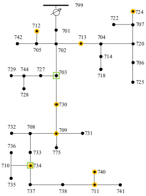
Numerical experiments were conducted on a modified IEEE 37-node test feeder to demonstrate the proposed model-free OPF. We used a single-phase variant of the original test feeder [24], with DERs connected at different locations. Fig. 1 shows the feeder diagram. Table I provides the configuration for these DERs, and the efficiency of the batteries is assumed to be 0.9.
| Node | PV Capacity (kVA) | Battery Capacity | ||||||
|---|---|---|---|---|---|---|---|---|
|
|
|
||||||
| 703 | N/A | 12 | ||||||
| 709 | 200 | N/A | ||||||
| 711 | N/A | |||||||
| 712 | N/A | |||||||
| 713 | N/A | |||||||
| 724 | N/A | |||||||
| 730 | N/A | |||||||
| 734 | 12 | |||||||
| 740 | N/A | |||||||
| Coefficients in the cost function (36b) | ||||||
|---|---|---|---|---|---|---|
| Value |
| Step sizes (control variables) | ||||
|---|---|---|---|---|
| Value |
| Step sizes (dual variables) | ||||||||
|---|---|---|---|---|---|---|---|---|
| Value |
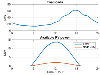
In simulation, the load and PV data were obtained from the real data in California [4]. They were smoothed and scaled to an appropriate magnitude for the considered distribution system. The total demand and available PV generation in a typical day are given in Fig. 2.
The described distribution system was simulated using Matpower [38], from where the feeder head active power and node voltages are obtained as system outputs. The output measurements were obtained by adding Gaussian noises to the simulated outputs; in particular,
| (42) |
where the random variable follows the normal distribution . In simulations, unless otherwise stated, , which is consistent with the standard phasor measurement units noise values [36, 12].
Algorithm parameters were configured as shown in Table II. For each local controller, the sine signal was chosen as the perturbation signal:
where the time step second; , with base power MVA; and the frequency was uniquely chosen from the range Hz.
VI-B Simulation Results
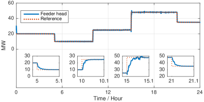
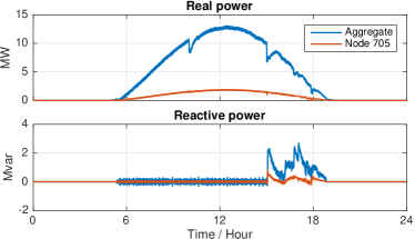
The results described here are based on the 24-hour simulation with the load and PV data given in Fig. 2. It is observed from Fig. 3 that the feeder head power nicely tracks the desired reference power and the DERs can respond quickly to unforeseen changes of the reference signal. The subplots on the bottom of Fig. 3 show the detailed response when the reference signal was changed. The power tracking is less accurate during hours, because the power tracking was conflicting with another objective of voltage regulation.
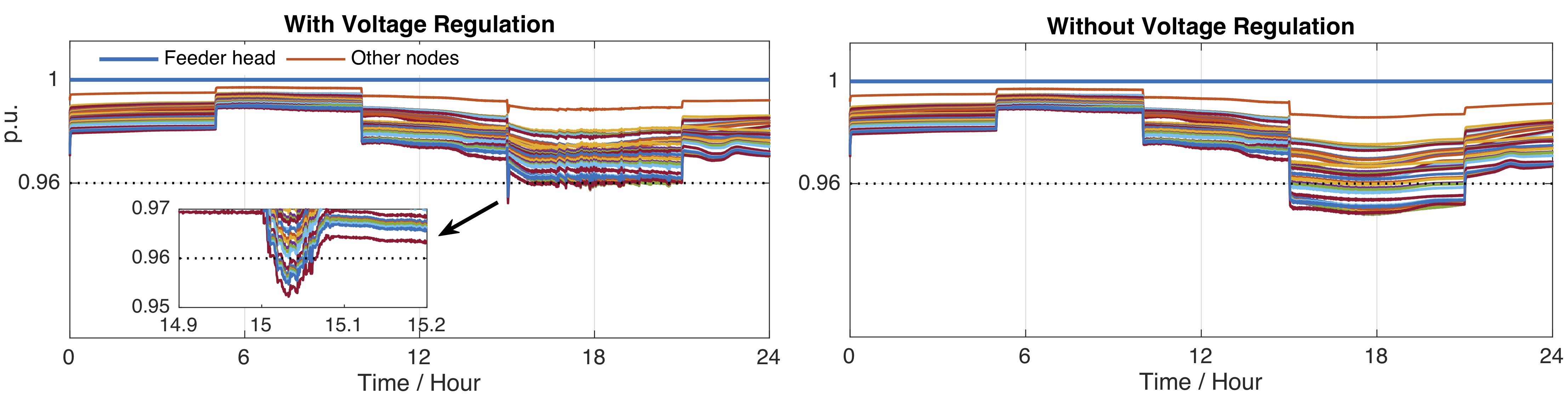
The performance of voltage regulation is illustrated in Fig. 5, which provides the comparison of node voltages with and without voltage regulation. The voltage lower limit was set to 0.96 p.u. At the time around hours, when some node voltages dropped below the limit, they were recovered quickly to normal values. In contrast, without regulation (no voltage limit), some node voltages stayed below 0.96 p.u. for the next 6 hours.
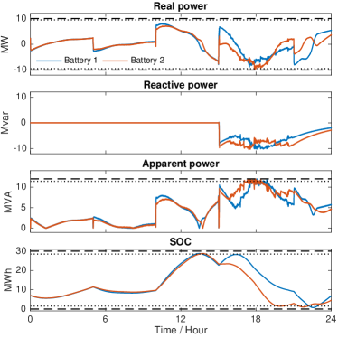
These grid services were provided through the control of battery and PV systems, whose behaviors are presented in Fig. 4 and Fig. 6, respectively. The feeder head power was controlled using the active power of DERs, mainly from batteries. The PV systems have its main objective of curtailment minimization, so the active PV power was merely increased because it is already near the maximal generation. But the active PV power can be largely curtailed when the system requested less power generation (e.g., at time 10, 15 hours). Because the active power of DERs is determined to track the reference feeder head power, the voltage regulation is mainly accomplished by the reactive power of DERs. At the time around 15 hours when some node voltages dropped below the lower limit, the reactive power from both batteries and PVs acted quickly to recover these voltages to the normal range.
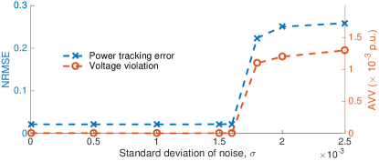
To study the impact of the measurement noise, we tested the proposed algorithm with different levels of noise, distinguished by the standard deviation of the noise signal in (42). Two metrics are used to quantify system performance. The normalized root mean squared error (NRMSE) is used to define power tracking performance:
The average voltage violation (AVV) is used to define voltage regulation performance:
where and are the number of nodes and simulation time steps, respectively; the operator projects a negative value to zero.
Fig. 7 shows simulation results of NRMSE and AVV. As the noise signal increases and crosses the point of , the control performance degrades significantly. It is because large measurement noise can suppress the exploration output and leads to inaccurate gradient estimation. One idea to address this issue is to increase the exploration signal to a reasonable magnitude. But the improvement space is limited because of practical system considerations. In that case, we can apply state estimation techniques to filter out measurement noises. It is beyond the scope of this paper and left to our future work.
VII Conclusions and Future Work
In this paper, we developed a model-free primal-dual method to track desired trajectories of networked systems. The algorithm leverages the zero-order deterministic estimation of the gradient with two function evaluations. We provided preliminary stability and tracking results, and illustrated an application of the method to real-time OPF in power systems.
Analysis of the exact iteration (18)-(19), with the projection performed at every time step, remains an interesting research topic. The promising direction here is to analyze the time-varying projected dynamics of the form (24). Also, analysis of the asynchronous model-free algorithm is important from the practical perspective. Finally, on the application side, it would be interesting to show the performance of the algorithm on a more dynamic scenario, including topology reconfigurations (e.g., due to natural disasters and attacks on the grid).
References
- [1] K. Ariyur and M. Krstic. Real-Time Optimization by Extremum-Seeking Control. Wiley-interscience publication. Wiley, 2003.
- [2] K. B. Ariyur and M. Krstić. Real Time Optimization by Extremum Seeking Control. John Wiley & Sons, Inc., New York, NY, 2003.
- [3] B. Awerbuch and R. Kleinberg. Online linear optimization and adaptive routing. Journal of Computer and System Sciences, 74(1):97 – 114, 2008. Learning Theory 2004.
- [4] J. Bank and J. Hambrick. Development of a high resolution, real time, distribution-level metering system and associated visualization, modeling, and data analysis functions. May 2013.
- [5] A. Bernstein, Y. Chen, M. Colombino, E. Dall’Anese, P. Mehta, and S. Meyn. Optimal rate of convergence for quasi-stochastic approximation. To appear, IEEE CDC and arXiv:1903.07228, Mar 2019.
- [6] A. Bernstein and E. Dall’Anese. Asynchronous and distributed tracking of time-varying fixed points. In 2018 IEEE Conference on Decision and Control (CDC), pages 3236–3243, Dec 2018.
- [7] A. Bernstein and E. Dall’Anese. Real-time feedback-based optimization of distribution grids: A unified approach. IEEE Transactions on Control of Network Systems, 6(3):1197–1209, Sep. 2019.
- [8] A. Bernstein, E. Dall’Anese, and A. Simonetto. Online primal-dual methods with measurement feedback for time-varying convex optimization. IEEE Transactions on Signal Processing, 67(8):1978–1991, April 2019.
- [9] A. Bernstein, C. Wang, E. Dall’Anese, J. Le Boudec, and C. Zhao. Load flow in multiphase distribution networks: Existence, uniqueness, non-singularity and linear models. IEEE Transactions on Power Systems, 33(6):5832–5843, Nov 2018.
- [10] S. Bhatnagar, M. C. Fu, S. I. Marcus, and I.-J. Wang. Two-timescale simultaneous perturbation stochastic approximation using deterministic perturbation sequences. ACM Trans. Model. Comput. Simul., 13(2):180–209, 2003.
- [11] V. S. Borkar. Stochastic Approximation: A Dynamical Systems Viewpoint. Hindustan Book Agency and Cambridge University Press (jointly), Delhi, India and Cambridge, UK, 2008.
- [12] M. Brown, M. Biswal, S. Brahma, S. J. Ranade, and H. Cao. Characterizing and quantifying noise in pmu data. In 2016 IEEE Power and Energy Society General Meeting (PESGM), pages 1–5, July 2016.
- [13] S. Bubeck and N. Cesa-Bianchi. Regret analysis of stochastic and nonstochastic multi-armed bandit problems. Foundations and Trends® in Machine Learning, 5(1):1–122, 2012.
- [14] T. Chen and G. B. Giannakis. Bandit convex optimization for scalable and dynamic iot management. IEEE Internet of Things Journal, 6(1):1276–1286, Feb 2019.
- [15] M. Colombino, E. Dall’Anese, and A. Bernstein. Online optimization as a feedback controller: Stability and tracking. IEEE Transactions on Control of Network Systems, pages 1–1, 2019.
- [16] E. Dall’Anese and A. Simonetto. Optimal power flow pursuit. IEEE Transactions on Smart Grid, 9(2):942–952, March 2018.
- [17] J. C. Duchi, M. I. Jordan, M. J. Wainwright, and A. Wibisono. Optimal rates for zero-order convex optimization: The power of two function evaluations. IEEE Transactions on Information Theory, 61(5):2788–2806, May 2015.
- [18] M. Fazlyab, C. Nowzari, G. J. Pappas, A. Ribeiro, and V. M. Preciado. Self-Triggered Time-Varying Convex Optimization. In Proceedings of the 55th IEEE Conference on Decision and Control, pages 3090 – 3097, Las Vegas, NV, US, December 2016.
- [19] A. D. Flaxman, A. T. Kalai, and H. B. McMahan. Online convex optimization in the bandit setting: Gradient descent without a gradient. In Proceedings of the Sixteenth Annual ACM-SIAM Symposium on Discrete Algorithms, SODA ’05, pages 385–394, Philadelphia, PA, USA, 2005. Society for Industrial and Applied Mathematics.
- [20] X. Gao, B. Jiang, and S. Zhang. On the information-adaptive variants of the admm: An iteration complexity perspective. Journal of Scientific Computing, 76(1):327–363, Jul 2018.
- [21] D. Hajinezhad, M. Hong, and A. Garcia. Zone: Zeroth order nonconvex multi-agent optimization over networks. IEEE Transactions on Automatic Control, pages 1–1, 2019.
- [22] A. Hauswirth, S. Bolognani, G. Hug, and F. Dörfler. Projected gradient descent on riemannian manifolds with applications to online power system optimization. In 2016 54th Annual Allerton Conference on Communication, Control, and Computing (Allerton), pages 225–232, Sep. 2016.
- [23] A. Hauswirth, I. Subotić, S. Bolognani, G. Hug, and F. Dörfler. Time-varying projected dynamical systems with applications to feedback optimization of power systems. In 2018 IEEE Conference on Decision and Control (CDC), pages 3258–3263, Dec 2018.
- [24] W. H. Kersting. Distribution system modeling and analysis. CRC press, 2006.
- [25] J. Kiefer and J. Wolfowitz. Stochastic estimation of the maximum of a regression function. Ann. Math. Statist., 23(3):462–466, 09 1952.
- [26] J. Koshal, A. Nedić, and U. Y. Shanbhag. Multiuser optimization: Distributed algorithms and error analysis. SIAM J. on Optimization, 21(3):1046–1081, 2011.
- [27] M. Krstić and H.-H. Wang. Stability of extremum seeking feedback for general nonlinear dynamic systems. Automatica, 36(4):595 – 601, 2000.
- [28] Y. Nesterov. Introductory Lectures on Convex Optimization: A Basic Course. Springer, 1 edition, 2014.
- [29] Y. Nesterov and V. Spokoiny. Random gradient-free minimization of convex functions. Foundations of Computational Mathematics, 17(2):527–566, Apr 2017.
- [30] L. Prashanth, S. Bhatnagar, N. Bhavsar, M. C. Fu, and S. Marcus. Random directions stochastic approximation with deterministic perturbations. IEEE Transactions on Automatic Control, 2019.
- [31] S. Rahili and W. Ren. Distributed continuous-time convex optimization with time-varying cost functions. IEEE Transactions on Automatic Control, 62(4):1590–1605, April 2017.
- [32] B. Shi, S. S. Du, W. J. Su, and M. I. Jordan. Acceleration via Symplectic Discretization of High-Resolution Differential Equations. arXiv e-prints, page arXiv:1902.03694, Feb 2019.
- [33] D. Shirodkar and S. Meyn. Quasi stochastic approximation. In Proceedings of the 2011 American Control Conference, pages 2429–2435, June 2011.
- [34] J. C. Spall. Multivariate stochastic approximation using a simultaneous perturbation gradient approximation. IEEE Transactions on Automatic Control, 37(3):332–341, March 1992.
- [35] H.-H. Wang and M. Krstić. Extremum seeking for limit cycle minimization. IEEE Transactions on Automatic Control, 45(12):2432–2436, Dec 2000.
- [36] L. Xie, Y. Chen, and P. R. Kumar. Dimensionality reduction of synchrophasor data for early event detection: Linearized analysis. IEEE Transactions on Power Systems, 29(6):2784–2794, Nov 2014.
- [37] J. Zhang, A. Mokhtari, S. Sra, and A. Jadbabaie. Direct runge-kutta discretization achieves acceleration. In Proceedings of the International Conference on Neural Information Processing Systems (and arXiv:1805.00521), pages 3904–3913, USA, 2018. Curran Associates Inc.
- [38] R. D. Zimmerman, C. E. Murillo-Sanchez, and R. J. Thomas. Matpower: Steady-state operations, planning, and analysis tools for power systems research and education. IEEE Transactions on Power Systems, 26(1):12–19, Feb 2011.