Proper Orthogonal Decomposition Analysis and Modelling of the wake deviation behind a squareback Ahmed body

Abstract

We investigate numerically the 3-D flow around a squareback Ahmed body at Reynolds number $Re=10^{4}$. Proper Orthogonal Decomposition (POD) is applied to a symmetry-augmented database in order to describe and model the flow dynamics. Comparison with experiments at a higher Reynolds number in a plane section of the near-wake at mid-height shows that the simulation captures several features of the experimental flow, in particular the antisymmetric quasi-steady deviation mode. 3-D POD analysis allows us to classify the different physical processes in terms of mode contribution to the kinetic energy over the entire domain. It is found that the dominant fluctuating mode on the entire domain corresponds to the 3-D quasi-steady wake deviation, and that its amplitude is well estimated from 2-D near-wake data. The next most energetic flow fluctuations consist of vortex shedding and bubble pumping mechanisms. It is found that the amplitude of the deviation is negatively correlated with the intensity of the vortex shedding in the spanwise direction and the suction drag coefficient. Finally, we find that despite the slow convergence of the decomposition, a POD-based low-dimensional model reproduces the dynamics of the wake deviation observed experimentally, as well as the main characteristics of the global modes identified in the simulation.

I Introduction

A surprisingly generic feature of the flow around symmetric bodies at high Reynolds numbers is the presence of permanent symmetry-breaking structures in the wake. These have been observed for the sphere [9], bullet [24] , the flat plate [2], as well as academic models for ground vehicles such as the Ahmed body [10] and the Windsor body [18]. The origin and dynamics of these structures has not been entirely elucidated, although they have been the object of several experimental and numerical studies. They appear to be connected to the first bifurcation observed at much lower Reynolds number (see [7], [8]). At higher Reynolds numbers, rapid switches between different quasi-stable states can be observed, as described by [22] and [1].

In the remainder of the paper, we will focus on the Ahmed body. Grandemange et al. [10] have established that the appearance of bi- or multi-stable states for the flow around a squareback Ahmed body depends on the value of the ground clearance and the aspect ratio of the body base. Pasquetti and Peres [16] carried out the first numerical simulation of the Ahmed body that was able to reproduce the steady wake deviation. However switches were not observed in Pasquetti and Peres’s simulation, since the typical time separating two switches is on the order of 1000 $U/H$ where $U$ is the incoming flow speed and $H$ the body characteristic height (see [14]). In more recent work Dalla Longa et al. [4] were able to integrate over sufficiently long times to capture the switch in the wake deviation. However they could only observe one switch, due to the still longer time scale separating two switches. They also applied Proper Orthogonal Decomposition and Dynamic Mode Decomposition (DMD, [25]) to extract the dynamics of the flow. Interaction of the near-wake recirculation zone with the surrounding shear layers is expected to play a part in the occurence of switches. They proposed that the switch is triggered by large hairpin vortices.

Volpe et al. [28] carried out a spectral analysis of the wake behind the squareback Ahmed body. Three low frequencies were identified in their experimental data: vortex-shedding modes with Strouhal numbers of 0.13 and 0.19 in the far wake, and wake pumping motion at a Strouhal number of 0.08 in the recirculation zone. Pavia et al. [17] have applied POD to both the experimental pressure and velocity field of a Windsor body to identify structures corresponding to the bi-stable modes and the dynamics of the switch. They identified pumping motion in the wake with a bi-stable vortical structure in the streamwise direction and derived a phase-averaged model that describes the switch between the quasi-stable states. They confirmed the observation made by Evrard et al. [5] and Cadot et al. [2] that the symmetric state corresponds to a lower drag.

Drag reduction through control of the flow asymmetry has been the object of several passive and active control strategies [14], [29], [1], [13], [27], [6], [23]. An important question is to determine how the different structures present in the flow contribute to the drag. A low-dimensional description and modelling of the large-scale structures could be beneficial for understanding, predicting and ultimately controlling the flow dynamics. Reduced-order models were developed by [1], [22] in order to control the deviation of the wake.

In the present work, we aim to provide a large-scale description of the flow by applying Proper Orthogonal Decomposition to a numerical investigation of the flow around a squareback Ahmed body at a Reynolds number of $Re=10^{4}$. The spanwise to vertical aspect ratio of the body is 1.18, so that bistability corresponds to two asymmetric states which are symmetric through reflection of the vertical mid-plane. Due to the long time scales separating switches, the change in the wake deviation could not be captured by the simulation. However, reflection symmetry was enforced artificially, so that we provide a description of the structures of the flow as a superposition of reflection-symmetric and reflection-antisymmetric modes.

The paper is organized as follows: section 2 presents the 3-D numerical configuration, while section 3 describes the specifics of Proper Orthogonal Decomposition. Section 4 presents a 2-D comparison of the numerical simulation and an experimental configuration corresponding to the same geometry but a higher Reynolds number, section 5 presents a 3-D POD analysis of the structures in the full configuration; a POD-based low-dimensional model is constructed in section 6 and compared with experimental and numerical results. A conclusion is given in section 7.

II Numerical configuration

Figure  1 presents the numerical configuration. The dimensions of the squareback Ahmed body are the same as the experimental configuration of Evrard et al. [5] i.e. $L=1.124m,H=0.297m,W=0.35m$. The ground clearance (distance from the body to the lower boundary of the domain) is 0.3H in the simulation. The Reynolds number based on the incoming velocity $U$, body height $H$ and fluid viscosity is $10^{4}$. The foremost and upper part body defines the reference position $(x=0,z=0)$. The plane $y=0$ corresponds to the mid-plane of the body. The domain extent in the streamwise (x), spanwise (y) and vertical (z) directions is $[-1,10]H\times[-2,2]H\times[-1.3,1.2]H$.

The code used is SUNFLUIDH, an in-house code developed at LIMSI based on a second-order finite volume approach which has been described for instance in [20]. The temporal discretization is based on a second-order backward Euler scheme. Diffusion terms are treated implicitly and convective terms are solved with an Adams-Bashforth scheme. The Poisson equation for the computation of pressure field is solved iteratively. We use $(512\times 256\times 256)$ grid points in respectively the longitudinal direction $x$, the spanwise direction $y$, and the vertical direction $z$. The Cartesian grid is refined close to surfaces. Periodic boundary conditions are used in the spanwise direction. No-slip velocity boundary conditions on the Ahmed body and on the ground are implemented by adjusting the size of the loops. The simulation was initialized from a uniform condition. About 100 time units based on the upstream velocity $U$ and body height $H$ were necessary for the flow to develop and statistical convergence to be reached. We note that all times will be expressed in those units in the remainder of the paper. All lengths will be made nondimensional with the body height $H$.

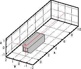
Figure 1: Numerical configuration. The Ahmed body and the recirculation zone behind it are idenfied by a surface of zero streamwise velocity. The streamwise, spanwise and wall-normal positions are referred to as $x$, $y$, $z$. The length, width and height of the body are respectively $L$, $W$ and $H$. The origin of the axes is taken at the top and foremost position of the Ahmed body in the vertical symmetry plane.

III Proper Orthogonal Decomposition

The main tool of analysis used in this paper is Proper Orthogonal Decomposition (POD) [15]. The field on a domain $\Omega$ is written as a superposition of spatial modes

$$\underline{u}(\underline{x},t)=\sum_{n}\tilde{a}_{n}(t)\underline{\phi}_{n}(\underline{x})$$ (1)

where the modes are orthogonal (and can be made orthonormal), i.e

$$\int\underline{\phi}_{n}(\underline{x}).\underline{\phi}_{m}(\underline{x})d\underline{x}=\delta_{nm}.$$

The modes can be ordered by decreasing energy $\lambda_{1}\geq\lambda_{2}\geq\ldots\geq\lambda_{n}=<\tilde{a}_{n}\tilde{a}_{n}>$, where $<.>$ represents a time average. The amplitudes $\tilde{a}_{n}$ can be obtained by projection of the velocity field onto the spatial modes:

$$\tilde{a}_{n}(t)=\int_{\Omega}\underline{u}(\underline{x},t).\underline{\phi}_{n}(\underline{x})d\underline{x}.$$ (2)

In the remainder of the paper we will consider normalized amplitudes $a_{n}=\tilde{a}_{n}/\sqrt{\lambda_{n}}.$

In all that follows POD is implemented following the method of snapshots [26] which is based on computing the autocorrelation between the different samples of the field obtained at times $t_{i},i=1,\ldots,N$:

$$C_{ij}=\frac{1}{N}\int_{\Omega}\underline{u}(\underline{x},t_{i}).\underline{u}(\underline{x}^{\prime},t_{j})d\underline{x},$$

and extracting the eigenvalues $\lambda_{n}$ and temporal eigenvectors $A_{in}=a_{n}(t_{i})$ such that

$$CA=\lambda A.$$ (3)

The spatial modes can then be reconstructed using

$$\tilde{\underline{\phi}}_{n}(\underline{x})=u(\underline{x},t_{i})A_{in}$$ (4)

and renormalizing ${\underline{\phi}}_{n}(\underline{x})=\frac{1}{N_{n}}\tilde{\underline{\phi}}_{n}(\underline{x})$ where

$$N_{n}^{2}=\int\tilde{\underline{\phi}}_{n}(\underline{x}).\tilde{\underline{\phi}}_{n}(\underline{x})d\underline{x}.$$ (5)

Different spatial domains, as well as different quantities will be considered in the decomposition. In section 4, we will limit the analysis to 2-D velocity fields in the near-wake region in order to match the data of Evrard et al. [5]. In section 5, we will apply POD to the full 3-D velocity field to the full numerical domain.

A key ingredient of the procedure is the definition of the data set. Cross-sections of the time-averaged streamwise velocity in the mid-height plane $z=-0.5$ and the vertical mid-span plane $y=0$ are represented in figure  2. We observe a steady deviation of the wake in agreement with previous observations [16]. This deviation is breaking the reflection symmetry with respect to the vertical mid-plane. However the equations are symmetric - for each flow realization, the flow obtained by symmetry with respect to the vertical midplane is also a possible solution. Following recommendations in  [11], an enlarged dataset enforcing the statistical symmetry could then be created as follows: for each snapshot of the original dataset, a symmetrized snapshot corresponding to the image of the snapshot by the reflection symmetry was created. The size of the new data set was therefore twice that of the original one. By construction, POD modes are thus either symmetric or antisymmetric with respect to the vertical midplane $y=0$, so that the amplitude of a POD mode for a given snapshot of the original dataset is either identical or opposite to that on the symmetrized snapshot. This allows us to break down flow patterns into symmetric and antisymmetric components.

Figure 2: Streamwise velocity contours of the mean flow; left) horizontal plane at mid-height $z=-0.5$; right) vertical mid-plane at $z=0$.

We emphasize that individual POD modes are different from coherent structures. A coherent structure typically corresponds to local patterns identified in a realization. POD modes are defined over the full domain chosen for decomposition, and every single realization contains a combination of modes. A coherent structure will therefore correspond to a combination of a few POD modes, which may be restricted to a portion of a spatial domain. As a consequence of the data enlargement procedure we have adopted, the mean flow of the simulation does not correspond to one single mode but to the sum of the first two modes representing respectively the symmetric and the antisymmetric part of the mean flow.

IV 2-D POD: Comparison with the experiment

In this section we apply POD analysis in the near-wake to the same variables defined over the same domain in both the experiment and the numerical simulation, i.e. the streamwise and the spanwise velocity components $u$ et $v$ defined over the domain $L\leq x\leq L+1.2H$, $-0.6\leq y\leq 0.6H$. Details are indicated in table  1. The main differences are
(i) the Reynolds numbers considered, as $Re=4$ $10^{5}$ in Evrard’s experiment and $Re=10^{4}$ in our numerical simulation
(ii) the time resolution - which is $25H/U$ in the experiment versus 0.5H/U in the simulation.

Type	Re	$\Delta T$	snapshot number (original data set)
Simulation	$10^{3}$	0.5	150
Experiment	$4$ $10^{5}$	25.25	400

Table 1: Comparison between model and experiment

Results for the POD spectrum are shown in figure  3 and show a good agreement between the experiment and the simulation. The second mode represents about 35% of the total fluctuating horizontal kinetic energy in the wake $\sum_{p\geq 2}\lambda_{p}$ and the first eight modes capture more than 50%. Figure  4 compares the first four POD modes for the experiment and the simulation. The first mode represents a cross-section of a toroidal-like structure constituting the recirculation bubble. The second mode corresponds to a single vortical structure located in the recirculation bubble close to the rear of the body and sweeping fluid from one side of the wake to the other. It represents the wake deviation. Overall a good agreeement is observed between all the modes found in the experiment and those found in the simulation.

Figure  5 shows for both the experiment and the simulation the corresponding amplitudes (normalized by the square root of the eigenvalue) of the modes represented in figure  4. The amplitudes of the first two modes in the simulation (figure  5 right) display small oscillations around a constant positive value. In the experiment (figure  5 left), the amplitude of the first mode oscillates near a constant positive value, while the amplitude of the second mode changes sign several times, which corresponds to a switch in the wake asymmetry.

We can also see from figure  4 that mode 3 is symmetric and mode 4 is antisymmetric. Mode 3 consists of a longitudinal converging (or diverging, depending on the sign of the amplitude) motion at the extremity of the recirculation bubble, which could be associated with wake pumping i.e successive enlargment and shrinking of the recirculation region. Mode 4 consists of three vortical structures - one larger structure extending across the wake and located close to the rear of the body, and two smaller ones, both rotating in the opposite direction, on each side of the recirculating bubble. Its action is therefore to distort the recirculation bubble in the spanwise direction. Since the PIV results are not resolved in time and the simulation total time is relatively short, it is difficult to compare directly time evolutions. However histograms of the amplitudes can be compared in figure  6 (we note that only the amplitudes corresponding to the original set of snapshots are shown). We can see that there is a relatively good agreement between the experiment and the simulation.

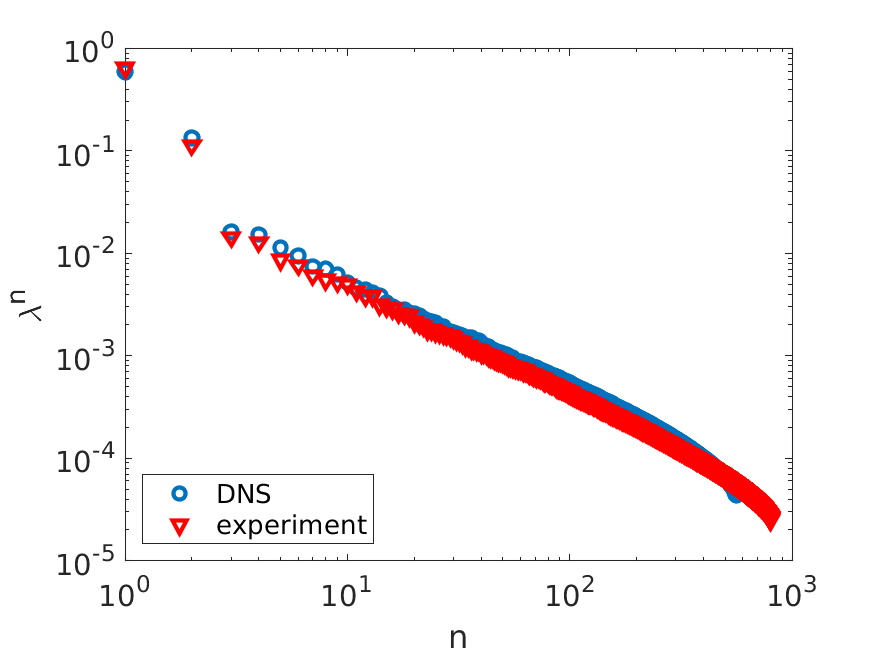
Figure 3: Near-wake 2-D POD spectrum in the simulation and experiment.

n=1	n=2	n=3	n=4

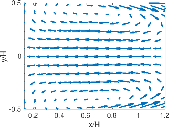
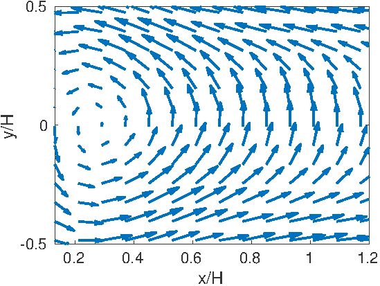
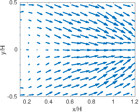
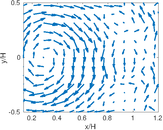
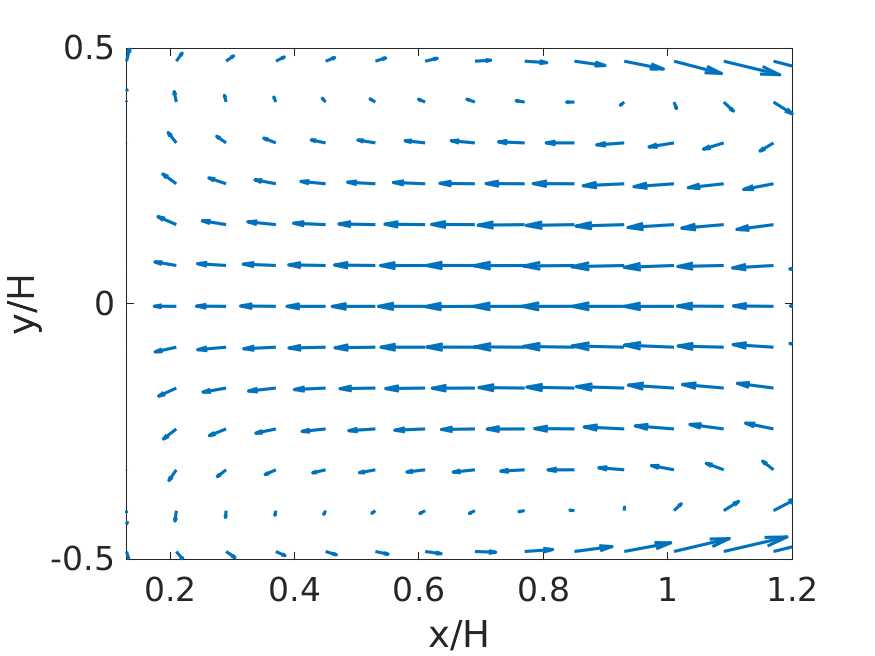
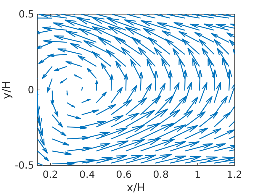
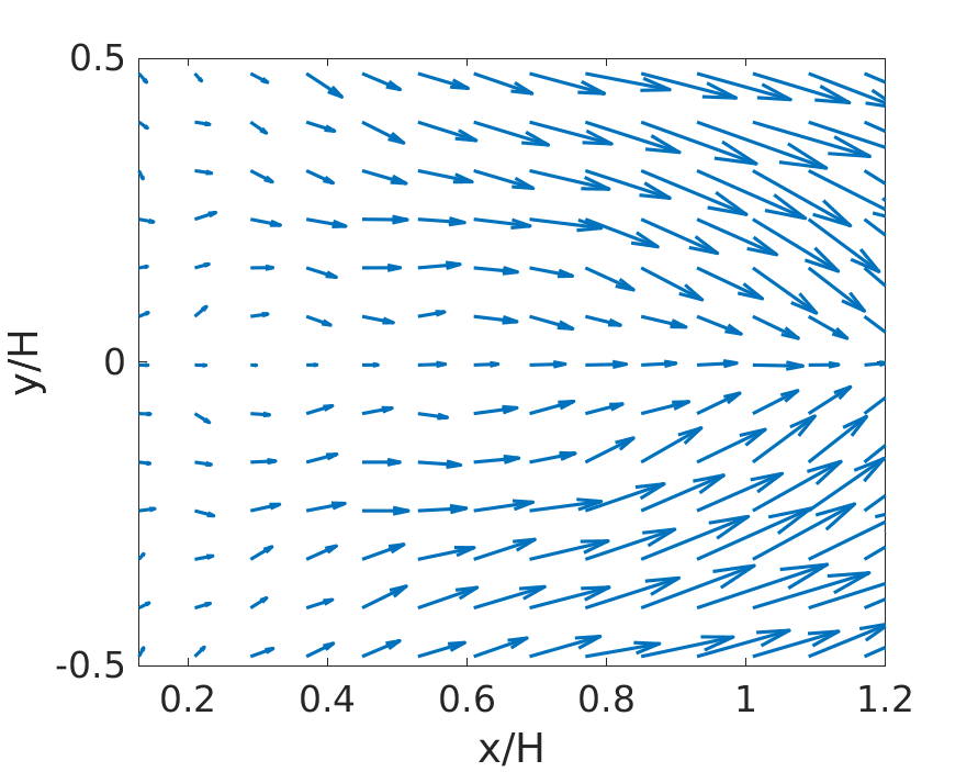
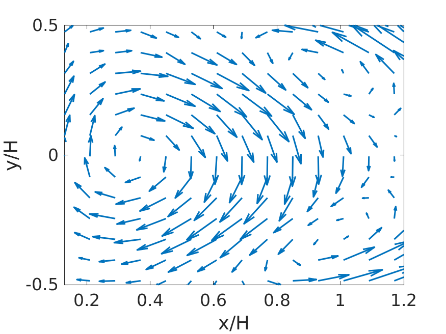
Figure 4: 2-D wake POD modes 1 to 4; top row: simulation; bottom row: experiment.

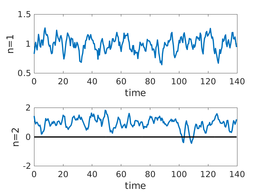
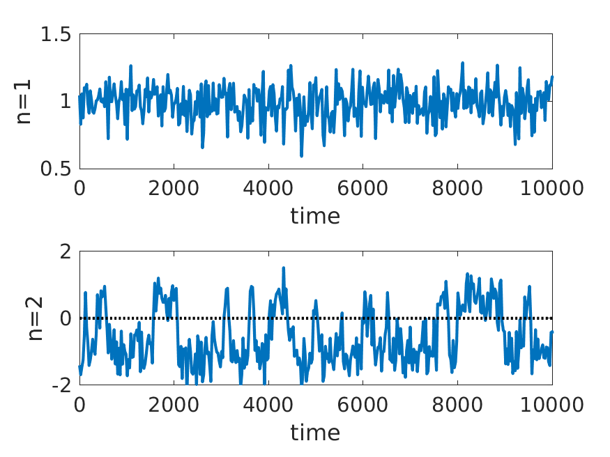
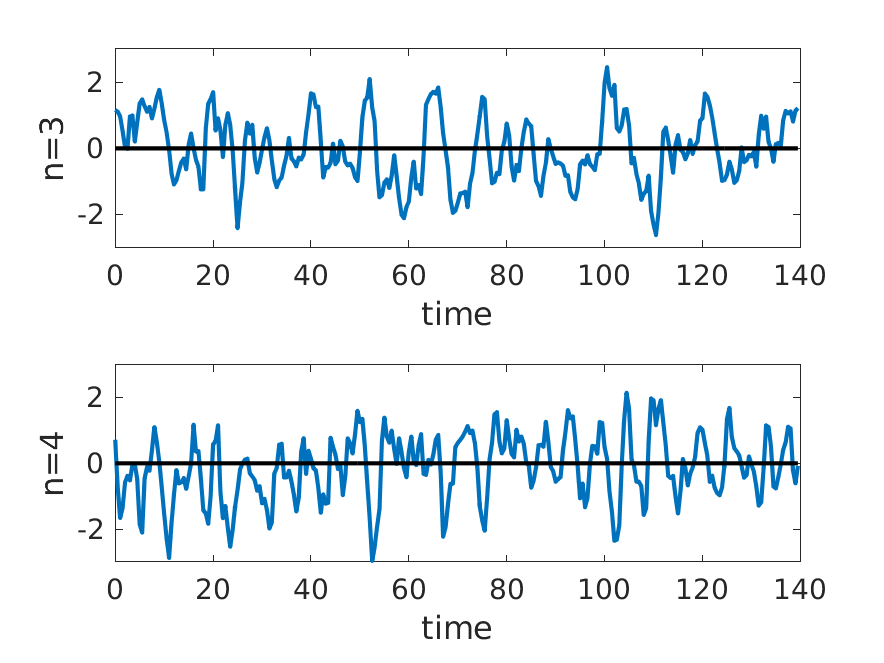
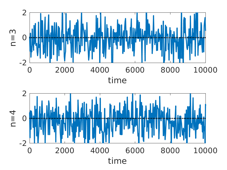
Figure 5: Amplitudes of 2-D POD modes 1 to 4 (from top to bottom); left) simulation; right) experiment.

n=1	n=2	n=3	n=4

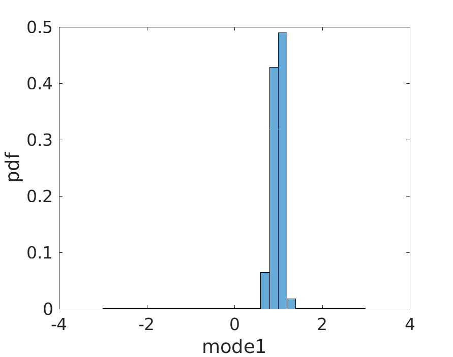
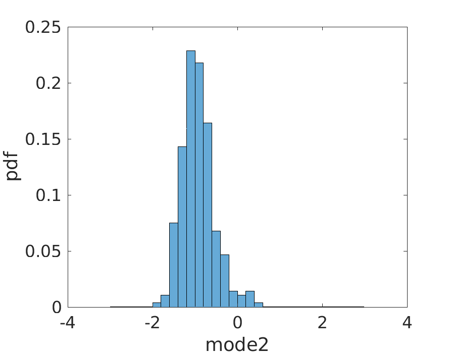
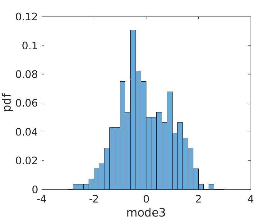
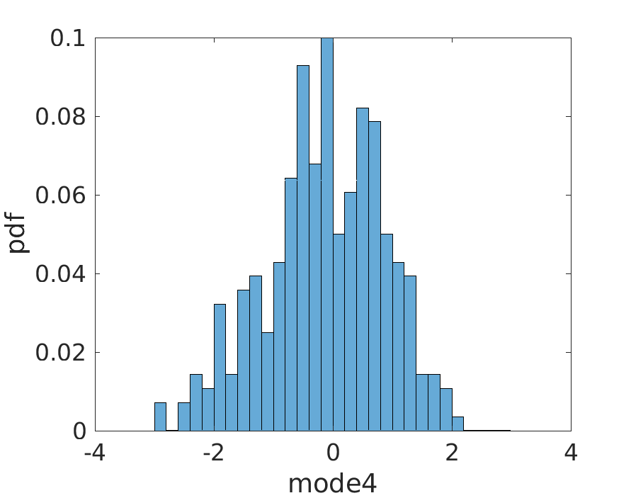
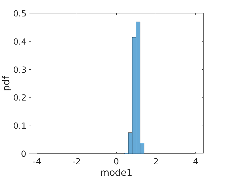
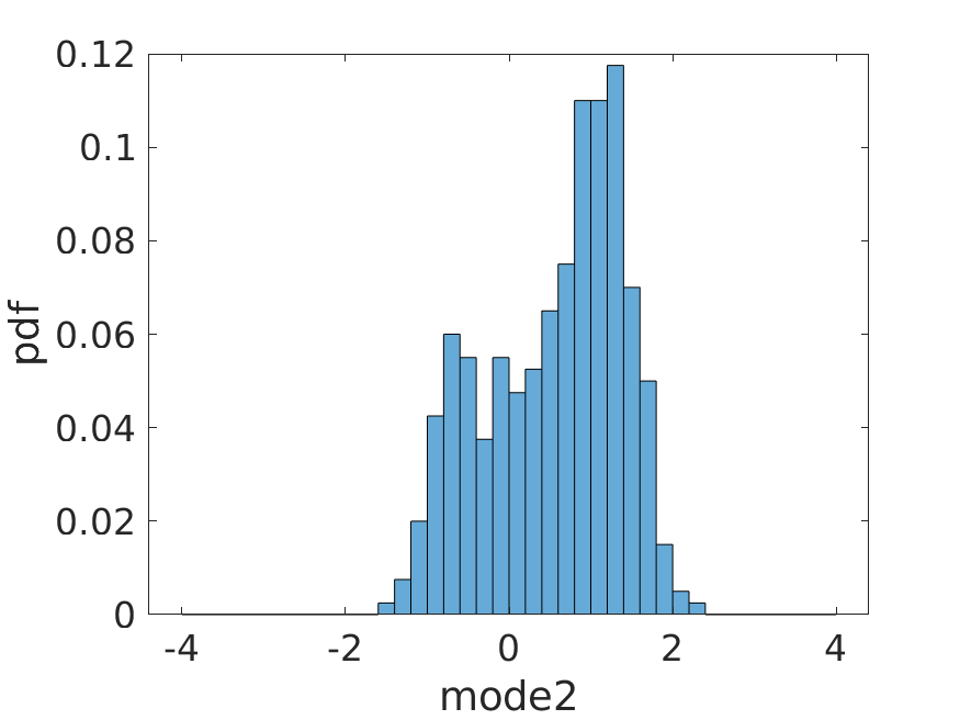
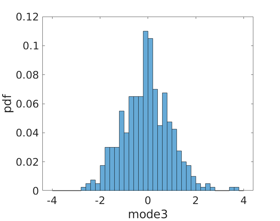
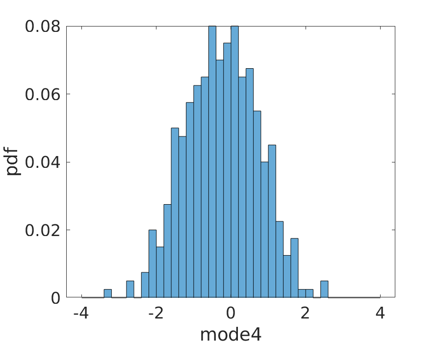
Figure 6: Histogram comparison of 2-D POD modes 1 to 4 (from left to right); top row: simulation; bottom row: experiment.

The next four order modes in the simulation, shown in figure  7, also present similarities with the modes in the experiment. Modes 5 and 8 are antisymmetric and consist of vortical motions respectively dominant on the inner part and the outer part of the recirculation. Modes 6 and 7 are symmetric and consist of two counter-rotating vortical structures, extending over the full recirculation length and located on each side of the wake. Given the differences in Reynolds number and time resolution, the agreement is remarkable and suggests that the most energetic structures have common features over a wide range of Reynolds numbers.

The spectral content of the temporal coefficients is presented in figure  8. All modes are characterized by low frequencies. The two red and black lines respectively correspond to the frequencies 0.08 and 0.2. Modes 3 and 7, which are both symmetric, are characterized by a dominant frequency around 0.08, while mode 4, 5 and 6, which are antisymmetric, are characterized by a frequency of 0.2. This frequency, which is associated with vortex shedding, can be identified most clearly in modes 5 and 6. Mode 8 is characterized by a mixture of frequencies.

n=5	n=6	n=7	n=8

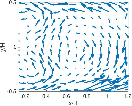
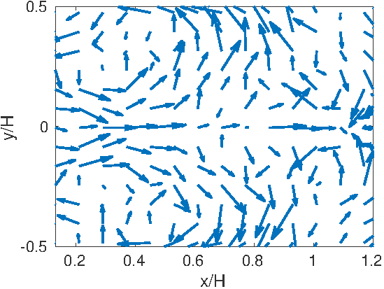
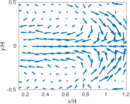
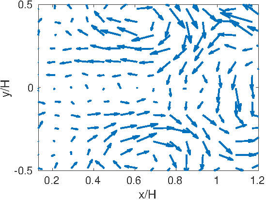
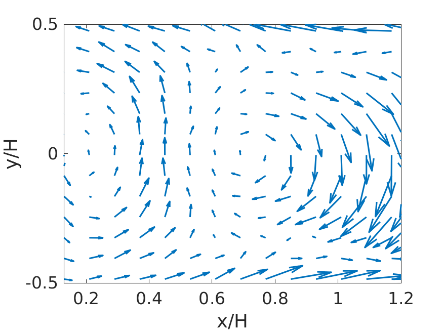
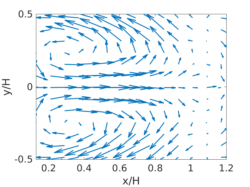
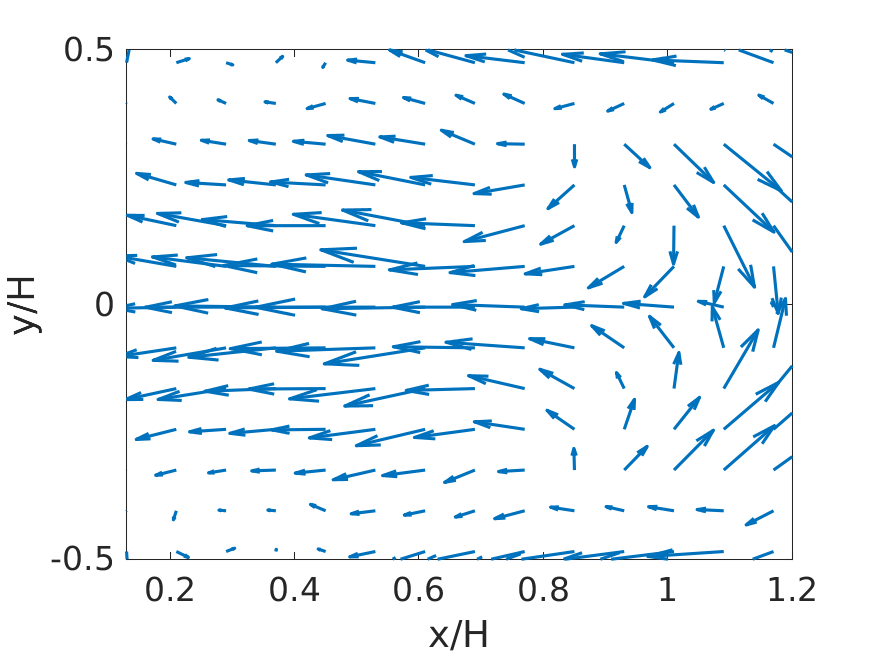
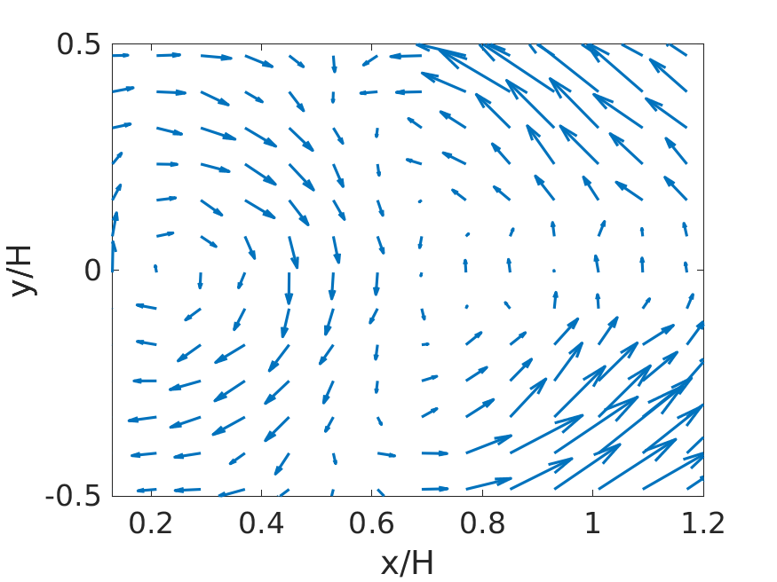
Figure 7: 2-D wake POD modes 5 to 8; top row: simulation; bottom row: experiment.

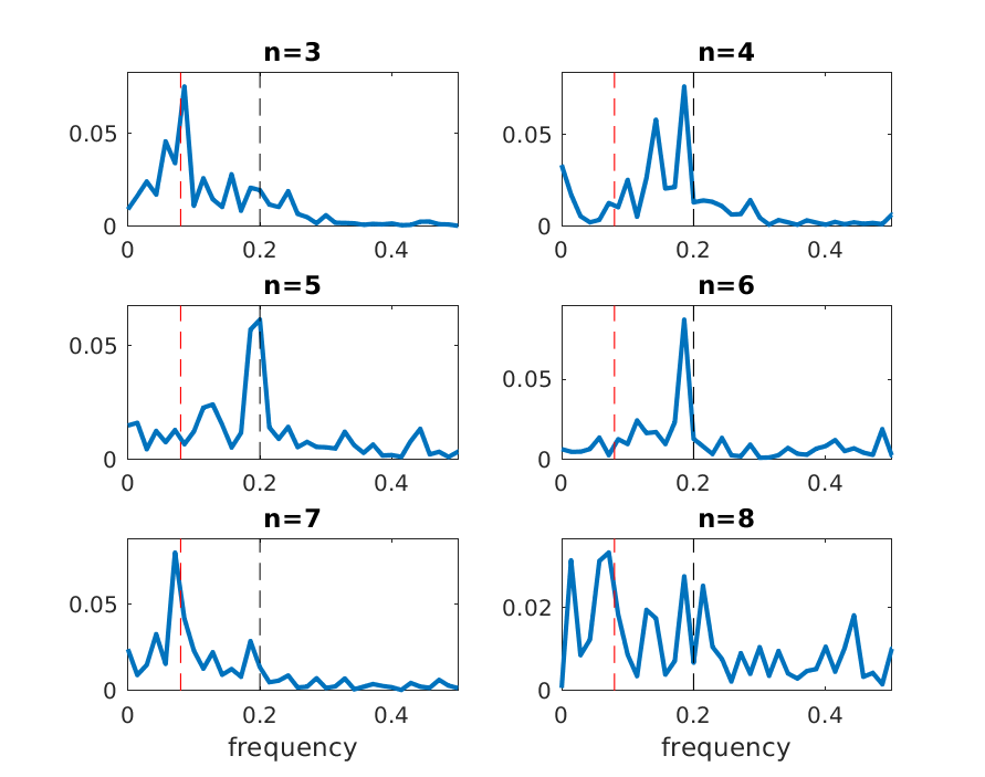
Figure 8: 2-D POD amplitude power spectral density $|\hat{a}_{n}|^{2}$ for modes 3 to 8 - the red and black dashed lines respectively correspond to the frequencies 0.08 and 0.2.

V 3-D POD

To investigate the flow structure and dynamics in more detail, POD is applied to the full 3-D velocity field over the entire computational domain. The eigenvalue spectrum is shown in figure  9. The first 3-D mode, which coincides with the mean flow, is much more energetic than the other modes compared with 2-D analysis (figure  3) since the entire domain contains a large steady contribution of the kinetic energy outside the wake. Due to the extent of the spatial domain, the convergence of the fluctuations is much slower than in the 2-D wake measurements. The second mode represents only 8% of the total fluctuating kinetic energy $\sum_{p\geq 2}\lambda_{p}$, which is equivalent to the combined energy of the next eight most energetic modes. We note that the modes 3 to 6 have nearly similar eigenvalues. This reflects the fact that the physical structures are global, three-component modes defined over the full domain, linking the upstream flow, the four boundary layers along the body, the near and the far wake. Figure  10 shows the projection of an instantaneous velocity field on the first ten modes and the difference between the full field and its projection. It is clear that only the large scales are captured by the projection. One can see that most of the unresolved modes (which represent the major portion of the total kinetic energy) are located in the boundary layers, the shear layers and the far wake.

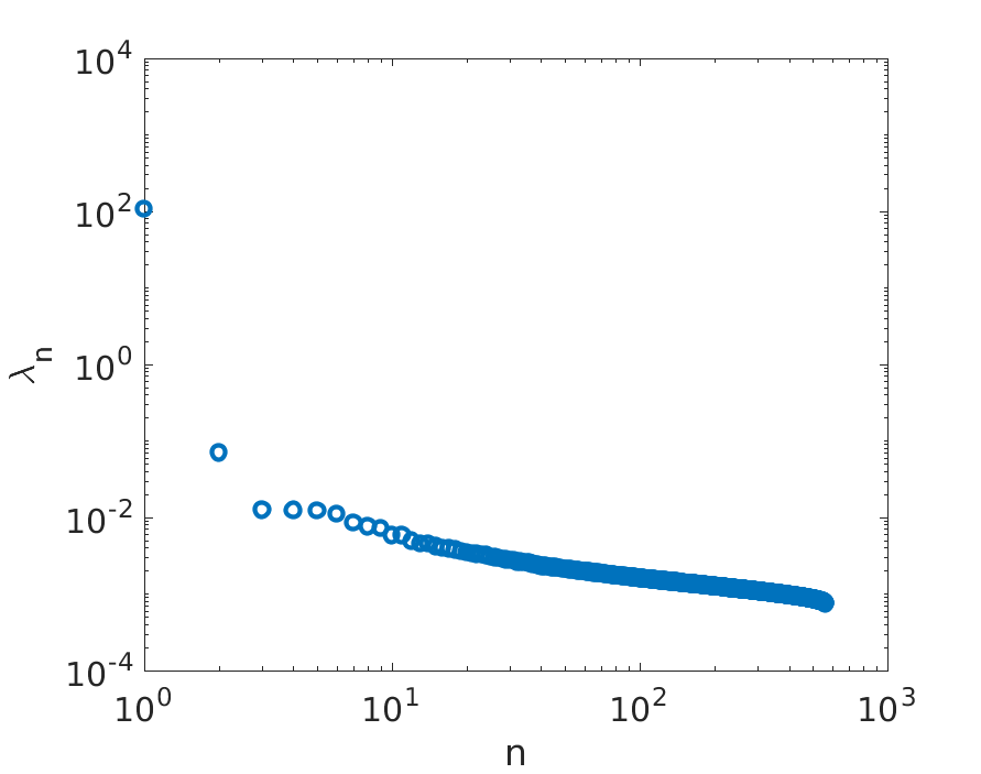
Figure 9: 3-D POD eigenvalue spectrum.

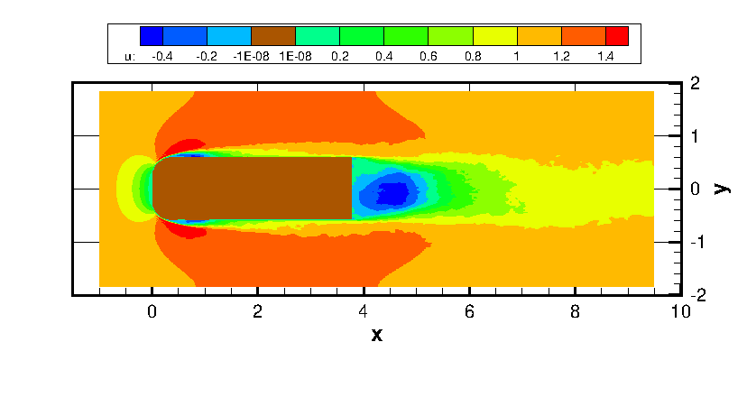
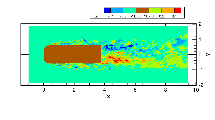
Figure 10: Streamwise velocity contours on mid-height plane $z=-0.5$; top : projection of an instantaneous field $\underline{u}$ onto the first ten modes $u_{recons}=\sum_{n=1}^{10}a_{n}(t)\underline{\phi}(\underline{x})$ where $a_{n}=\int\underline{u}(\underline{x},t).\underline{\phi}(\underline{x})d\underline{x}.$; bottom: difference field $|u-u_{recons}|$.

We now investigate the properties of the POD modes. For spatial characteristics, we represent in figures  11 and  14 the streamwise velocity contour of the 3-D POD modes in both a horizontal cross-section at mid-height $z=-0.5$, and in a vertical plane located in an off-center spanwise location $y=-0.4$ (since asymmetric motions will cancel on the symmetry plane). The first two spatial modes are shown in figure  11. Although the representation of the first two POD modes in 2-D and 3-D is different (figures  4 and  11), it can be shown that the restriction of the first two 3-D POD modes to the cross-section of the wake is similar to the 2-D POD results, which is not entirely surprising since they are expected to represent the symmetric and antisymmetric part of the time-averaged velocity field.

One can see in figure  12 that the temporal evolution of the first two 3-D POD modes is slightly different from that of the 2-D POD coefficients. Unlike its 2-D counter part (figure  5 right), the amplitude of the first 3-D POD mode is essentially constant, which shows the statistical convergence of the database. Moreover, the amplitudes of the second 2-D and 3-D mode present some discrepancies, but the correlation between the mean deviation coefficient $a_{2}^{2d}$ and $a_{2}^{3d}$ is 0.6, which indicates that the 2-D measurements are able to describe reasonably well the evolution of the 3-D deviation mode. However, although the amplitude of 2-D POD mode 2 changes sign, the corresponding 3-D POD amplitude $a_{2}^{3d}$ always remains positive. This means that there are no global switches in the total wake deviation although a local planar measure may indicate otherwise. In both cases, their corresponding spectrum indicates fluctuations at low frequencies thus confirming their very long-time dynamics evolution. In addition to its permanent asymmetry, the POD mode 2 corresponds to the very low frequency global mode as reported in [22, 23] for an axisymmetric body and responsible for the bistable dynamics found in [9] for the Ahmed body. To get a better insight into the action of the global deviation mode, figure  13 compares streamlines in the recirculation zone for the symmetrized mean field (mode 1) and the mean field (modes 1 and 2). We can see that the effect of the global deviation is to gather the streamlines around one of the base diagonals.

n=1
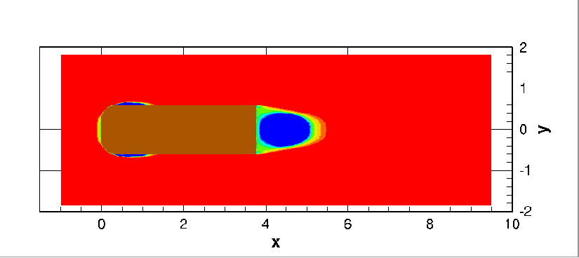
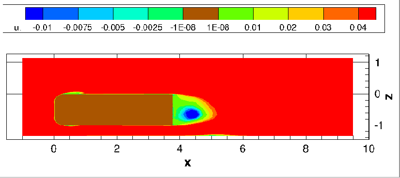
n=2

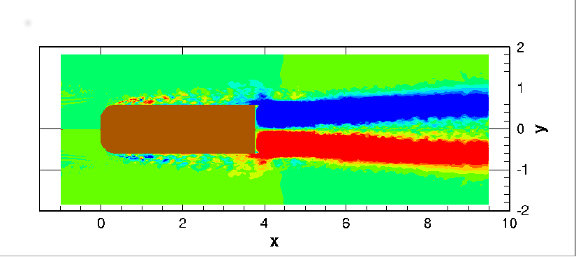
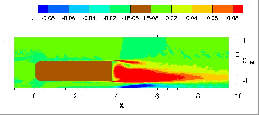
Figure 11: Streamwise velocity contours of 3-D POD modes 1 (top row) and 2 (bottom row); left) horizontal section at mid-height $z=-0.5$; right) vertical section at $y=-0.4$.

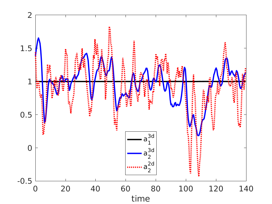
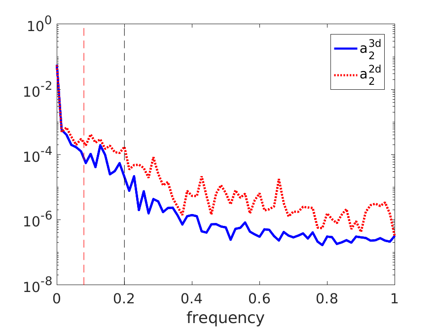
Figure 12: Left) amplitudes of the first two POD modes; right) power spectral density of the quasi-steady deviation mode $|\hat{a}_{2}|^{2}$ - the red and black lines respectively correspond to the two frequencies 0.08 and 0.2.

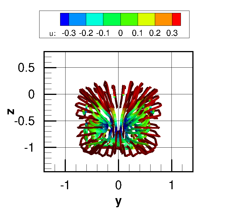
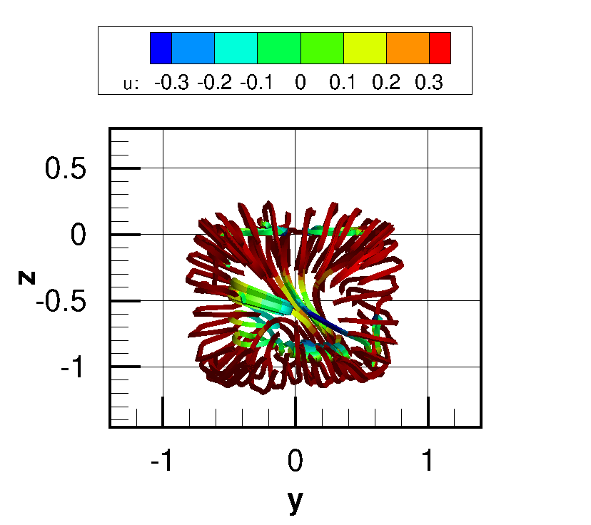
Figure 13: Streamlines of the field viewed from downstream left) mode 1 $\sqrt{\lambda_{1}}\underline{\phi}_{1}$; right) combination of mode 1 and mode 2 $\sqrt{\lambda_{1}}\underline{\phi}_{1}+\sqrt{\lambda_{2}}\underline{\phi}_{2}$ .

Modes 3 and 4 are antisymmetric modes which display a periodicity in the streamwise direction (figure  14). The time evolution of these modes is quasi-periodic as shown by the time series and the spectra in figure 15. The characteristics frequencies lie in the range 0.19-0.24, with a maximum around 0.19. This frequency matches satisfactorily the Kármán global mode observed for oscillations in the spanwise direction in (Grandemange et al. [9], Volpe et al. [28]). Similar observations are made for the symmetric modes 5 and 6 in figure  14 and the corresponding temporal properties in figure 15. Their spectra display a maximum around 0.23, that is ascribed to the vortex shedding (i.e. Kármán global mode) with oscillations in the vertical direction. The highest frequency corresponding to the small height and large frequency to the wider width of the body are in agreement with Grandemange et al. [9], Volpe et al. [28]. This is a general result for three-dimensional geometries (Kiya and Abe [12]).

The modes 7 and 8 in figure 14 are symmetric and clearly do not display streamwise periodicity. The action of mode 7 in the horizontal mid-plane is to modulate the bubble zone which is either inflated or shrunk, depending on the sign of $a_{7}$ (figure  15 left). When $a_{7}>0$, figure  14 shows that strong negative fluctuations are present in the bubble, which delays reattachment, and vice-versa. The spectra shown in figure  15 (right) show that both modes 7 and 8 are characterized by a strong energetic content at a frequency of 0.08, which suggests that these modes contribute significantly to the wake pumping, as characterized by Rigas et al. [24], Volpe et al. [28] and Pavia et al. [17].

Modes 9 and 10, which are antisymmetric (figure  14), are more difficult to interpret. As noted earlier, there is no guarantee that an individual POD mode corresponds to a well-defined physical mechanism. The spectra in figure 15 (right) show that modes 9 and 10 are characterized by a mixture of frequencies in an intermediate range 0.08-0.2, with a peak for both modes around 0.15. It is therefore likely that these modes correspond to a superposition of different physical processes.

As a summary, we find a clear correspondance between the POD modes and the main global modes that contribute to the wake dynamics reported in the literature: POD mode 2 is related to the very low frequency asymmetric or deviation global mode, modes 3 and 4 to vortex shedding with oscillation in the horizontal direction, modes 5 and 6 to vortex shedding with oscillations in the vertical direction, and modes 7 and 8 to (symmetric) wake pumping.

mode	u contour at $z=-0.5$	u contour at $y=-0.4$
n=3
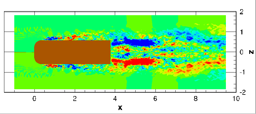
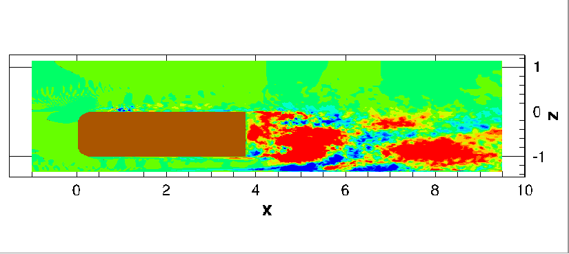
n=4
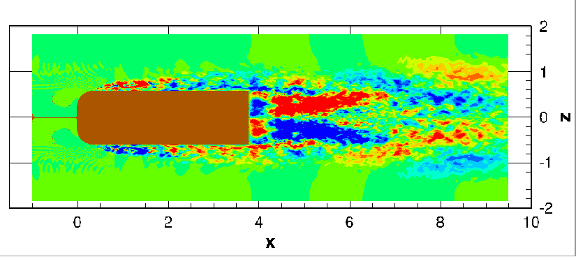
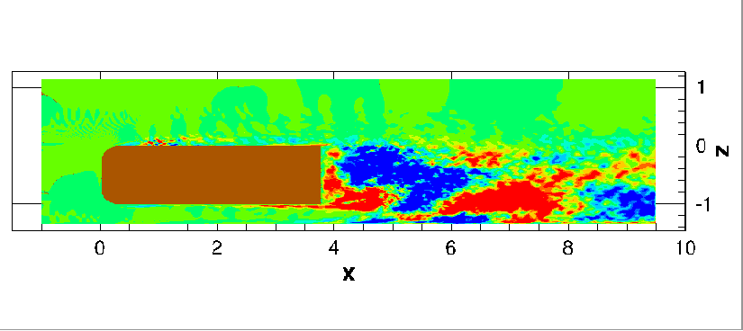
n=5
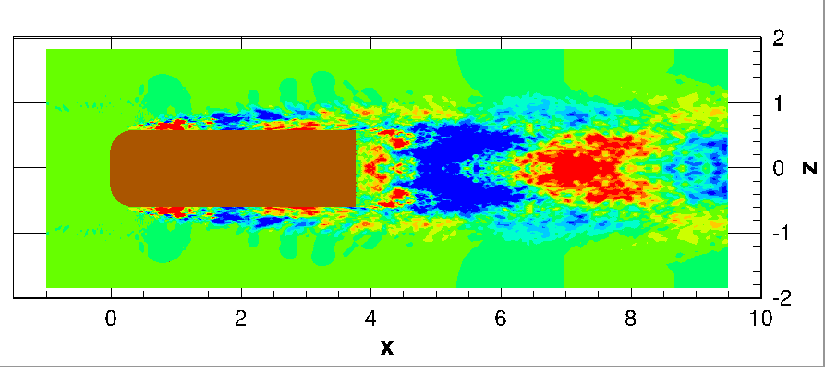
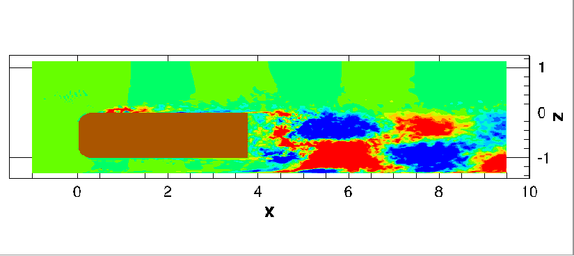
n=6
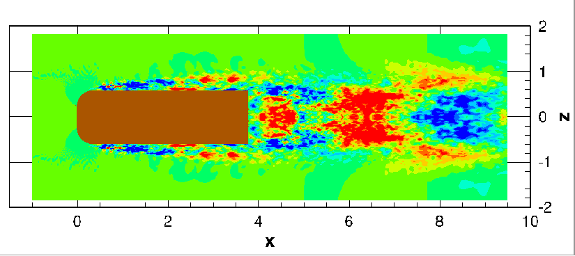
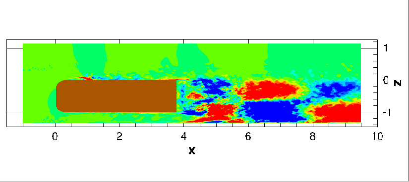
n=7
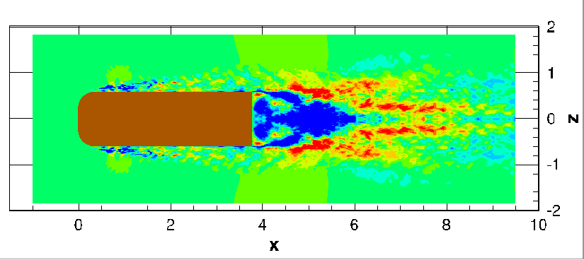
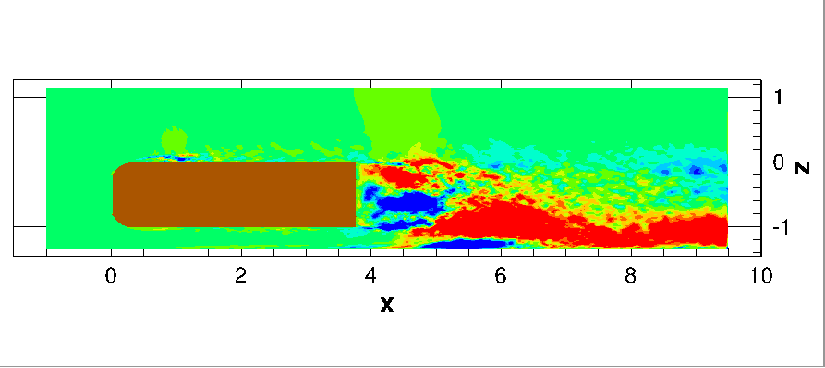
n=8
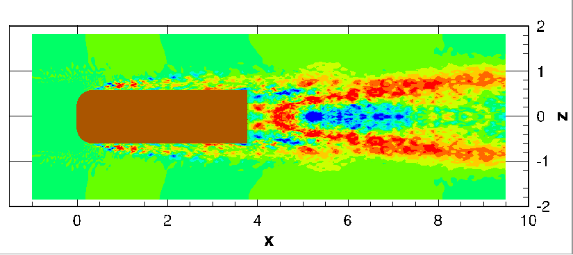
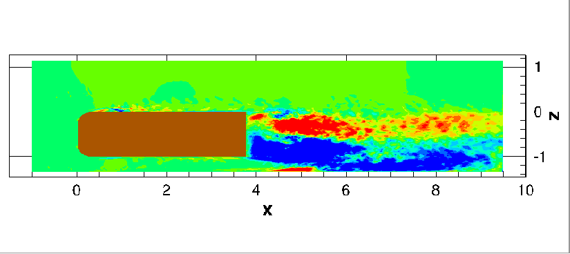
n=9
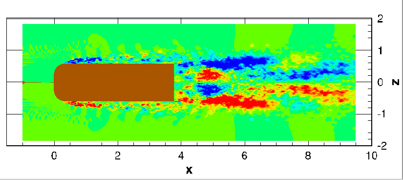
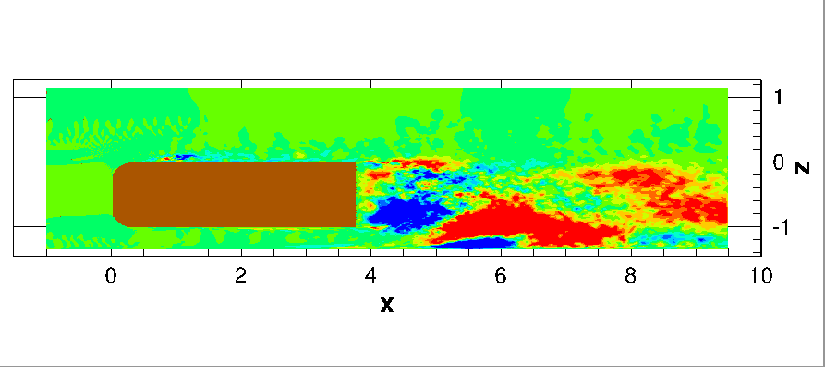
n=10

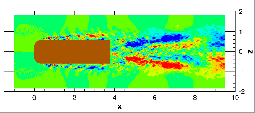
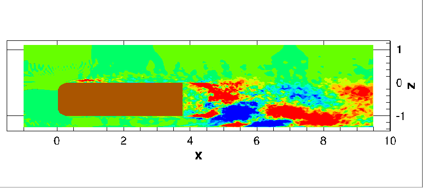
Figure 14: Streamwise velocity contours of 3-D POD spatial modes 3 to 10 (from top to bottom); left) horizontal section at mid-height $y=-0.5$; right) vertical section at $z=-0.4$.

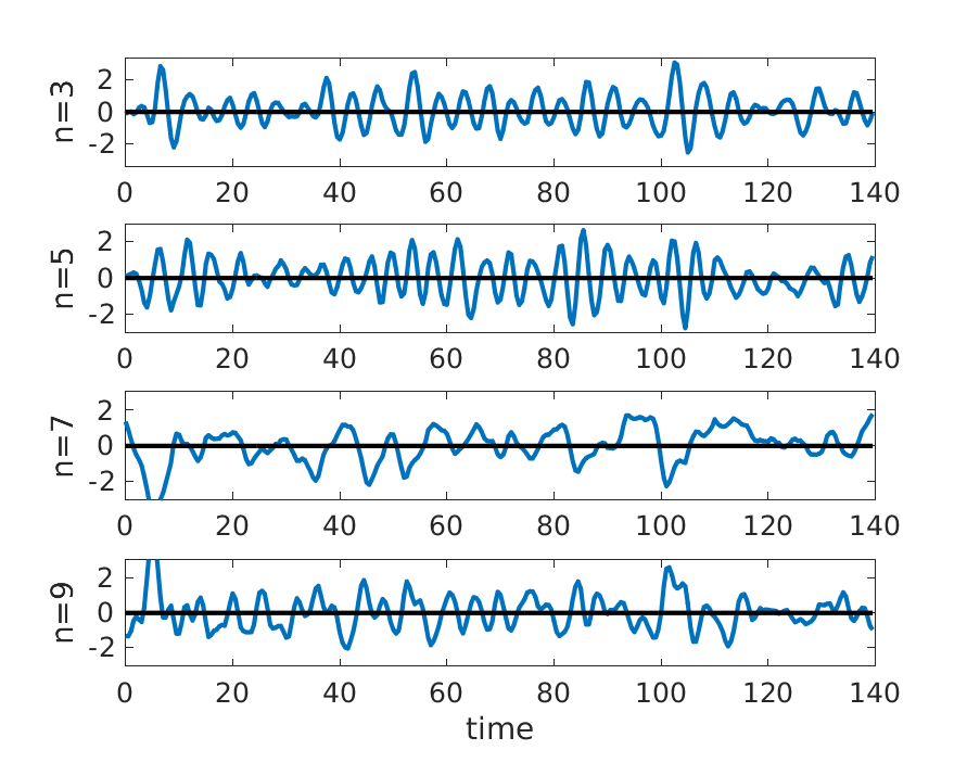
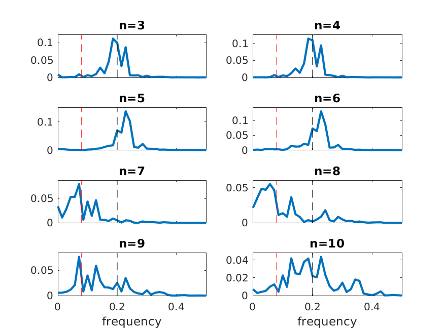
Figure 15: Left) amplitudes of the modes $a_{n}$, n=3, 5, 7, 9; right) power spectral density of the 3-D POD mode amplitudes in the simulation $|\hat{a}_{n}|^{2}$ - the red and black lines respectively correspond to the two frequencies 0.08 and 0.2.

The POD decomposition allows to investigate quantitatively the correlations between the global modes during the wake dynamics. We first compare the intensity of the deviation global mode given by ($a_{2}^{2}$) with the magnitude of vortex shedding in the horizontal (spanwise) and the vertical direction which can respectively be obtained with the sums of the amplitudes $r_{Kh}^{2}=a_{3}^{2}+a_{4}^{2}$ and $r_{Kv}^{2}=a_{5}^{2}+a_{6}^{2}$. We can see in figure  16 that minima of $a_{2}$ are associated with high energy in spanwise vortex shedding. The correlation coefficient between $|a_{2}|$ and ${|a_{3}|^{2}+|a_{4}|^{2}}$ is strongly negative (-0.6). Due to the three-dimensional nature of vortex shedding, spanwise and vertical shedding motions are correlated (0.48), so that a negative correlation is also obtained between $|a_{2}|$ and $a_{5}^{2}+a_{6}^{2}$ (-0.33). The negative correlation is consistent with the idea that a reduced asymmetry is accompanied by an increase in vortex shedding, which was observed in control experiments of [1] and [13].

The next step is to compare the evolution of the POD amplitudes with the base suction coefficient $C_{B}=-C_{pb}$ where the pressure coefficient $C_{pb}$ corresponds to the integral of the pressure over the base of the body, which is shown in figure  17 (left). Figure  17 (right) shows that the base suction coefficient is positively correlated with the amplitude of the wake deviation $a_{2}^{3d}$ with a positive delay of $\Delta tU/H\sim 2.5$ and with a maximum correlation coefficient of 0.55 ( we note that the correlation coefficient with the 2-D deviation mode $a_{2}^{2d}$ is 0.41. with a time delay of 4 time units). The time delay appears to have some significance as the correlation without time delay drops to 0.34. This suggests that the variations of the drag follow those of the mean deviation amplitude. This is in agreement with the idea that a drag reduction corresponds to a decrease in the quasi-steady wake asymmetry, as was observed by [2] and [17]. Figure  17 also shows that a correlation coefficient of -0.55 with a negative delay of $\Delta tU/H\sim-1.5$ is observed between the pressure and the amplitude of $a_{7}$. Unlike the previous case, the correlation remains about the same without no time delay (-0.51), so it is not possible to assign a physical relevance to the small time delay observed. As seen above, $a_{7}$ is associated with wake pumping: from figure  14 one can see in the near-wake that when $a_{7}>0$ there are more negative fluctuations within the zone, so that the size of the recirculation actually increases. This is consistent with the observation that the base suction coefficient decreases as the recirculation length increases.

In contrast, the correlation of the drag with the intensity of vortex shedding appears to be weaker (and negative).

The observations made above suggest the following picture: the flow is characterized by a quasi-steady wake deviation, vortex shedding modes and low-frequency wake pumping modes. The drag coefficient depends on the global (symmetric) size of the bubble, which is associated with wake pumping, as a longer bubble corresponds to a lower drag. It also depends on the magnitude of the quasi-steady wake asymmetry: a lower drag corresponds to a decrease of asymmetry, and to an increase in the intensity of vortex shedding, a negative correlation of vortex shedding in spanwise and vertical directions with both the quasi-steady deviation and the base suction coefficient.

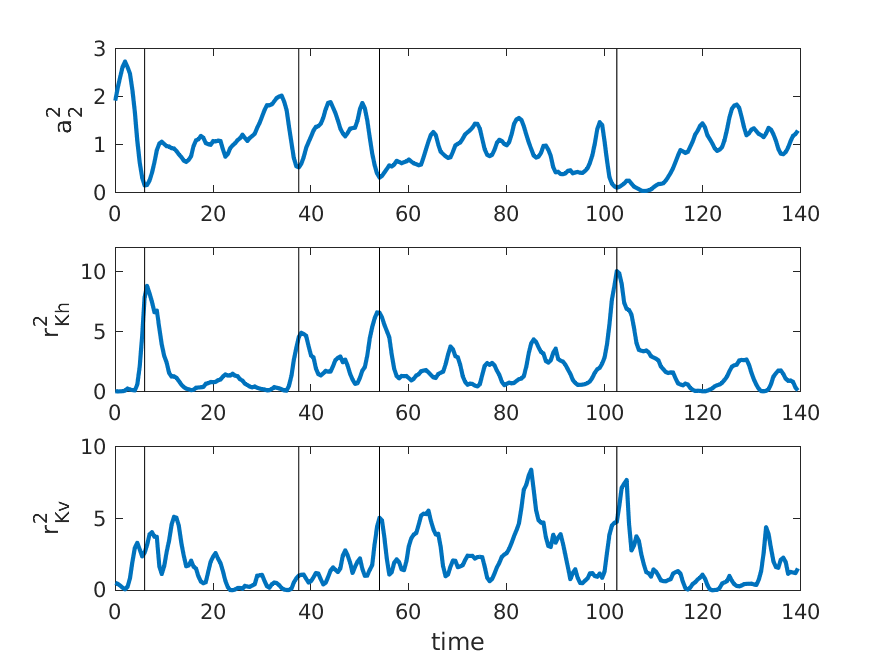
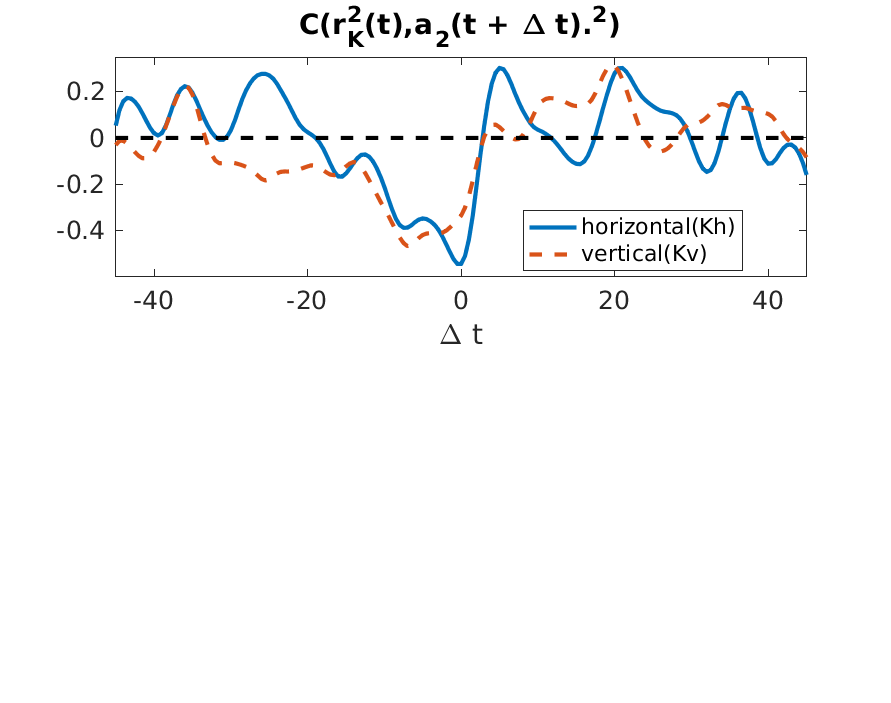
Figure 16: Left) energy of POD modes corresponding to quasi-steady deviation $a_{2}^{2}$, spanwise ($r_{Kh}^{2}=a_{3}^{2}+a_{4}^{2}$) and vertical ($r_{Kv}^{2}=a_{5}^{2}+a_{6}^{2}$) vortex shedding intensities - vertical lines correspond to minima of $a_{2}^{2}$; right) correlation coefficient between vortex shedding energy and quasi-steady deviation energy.

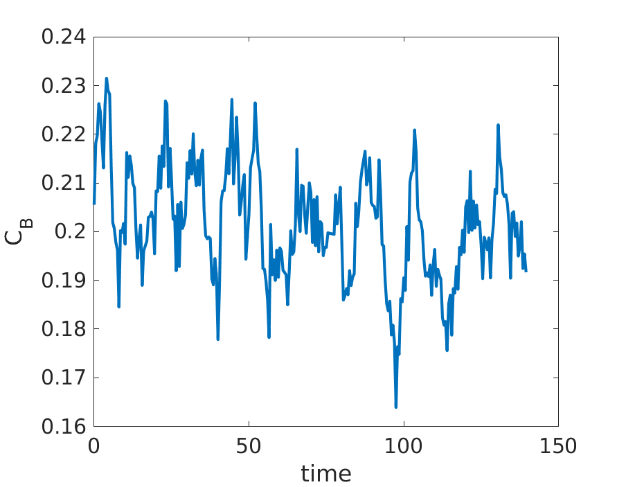
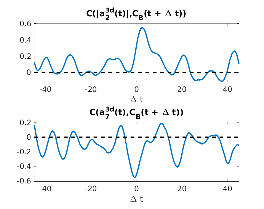
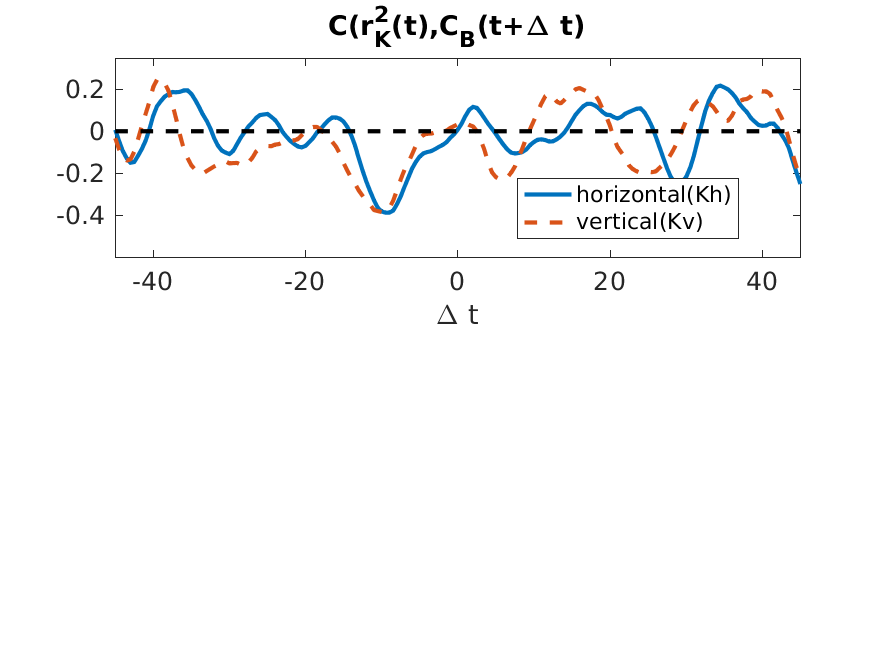
Figure 17: Left) base suction coefficient $C_{B}=-C_{p}$ obtained by integrating the pressure over the rear of the body; right) correlation between the base suction coefficient and the POD amplitudes corresponding to the steady deviation ($a_{2}$, top), wake pumping mode ($a_{7}$, middle) and vortex shedding modes ($r_{Kh,v}^{2}$, bottom).

VI Low-dimensional model

We now examine whether it is possible to model the behavior of the largest scales using a POD-based model, even if the scales considered represent only a fraction of the total fluctuating kinetic energy. Following the approach described in [19], [21], we build a low-dimensional model to reproduce the dynamics. We use a Galerkin approach to project the Navier-Stokes equations onto the basis of spatial modes for a selected truncation, and obtain a set of ordinary differential equations for the normalized amplitudes $a_{n}(t)$. The model is of the form

$$\dot{a}_{n}=L_{nm}a_{m}+Q_{nmp}a_{m}a_{p}+T_{n}.$$ (6)

where

• the linear terms contain the viscous dissipation

  $$L_{nm}=\int\nu\Delta\underline{\phi}_{m}.\underline{\phi}_{n}d\underline{x}.$$ (7)

  For the ten-mode truncation they form a diagonal matrix $L\sim-0.05I$ as indicated in table  2.

• $T_{n}$ is a closure term representing the contribution of the unresolved stresses (associated with the modes excluded from the truncation) to the evolution of the amplitude $a_{n}$.

• the quadratic terms $Q_{nmp}$ can be written in symmetric form as

  $$Q_{nmp}=\frac{\sqrt{\lambda_{m}\lambda_{p}}}{\lambda_{n}}\frac{1}{2}(2-\delta_{mp})\int(\underline{\phi}_{p}.\nabla\underline{\phi}_{m})+\underline{\phi}_{m}.\nabla\underline{\phi}_{p}).\underline{\phi}_{n}d\underline{x}.$$ (8)

  For the evolution equation of the amplitude $a_{n}$, $1<n\leq 10$, shown in equation ( 6), the interaction coefficient of $a_{n}$ with the mean mode, $Q_{nn1}$, is essentially independent of $n$ and its value is about 0.2. A physical interpretation of this is that each of the modes interacts directly and equally with the mean mode, in particular its strong shear layers.

Generally speaking, the magnitudes of the quadratic coefficients $Q_{nmp}$ provide insight into the interactions between the different modes. Table  3 contains the values of the quadratic coefficients $Q_{nm1}$ for $3\leq n,m\leq 10$. The dominant values which will be kept for the model are indicated in bold.

VI.1 Simplified model

We first consider a simplified version of the model by making the following assumptions:

• we assume that the first two modes $a_{1}$ and $a_{2}$ are constant.

• we neglect quadratic terms of small magnitude.

• we model the energy transfer to the unresolved modes by assuming that their effect is to compensate for the production term i.e the interaction with the mean shear (mode 1). This means that

  $$T_{n}=(-L_{n}-Q_{1nn}a_{1})a_{n}.$$ (9)

This leads to the following form for the model, which we will refer to as $M_{0}$:

$$\dot{a}_{1} = 0$$ (10)

$$\dot{a}_{2} = 0$$ (11)

$$\dot{a}_{3} = 0.91a_{4}$$ (12)

$$\dot{a}_{4} = -0.94a_{3}$$ (13)

$$\dot{a}_{5} = -1.09a_{6}+0.49a_{9}$$ (14)

$$\dot{a}_{6} = 1.22a_{5}$$ (15)

$$\dot{a}_{7} = -0.42a_{8}$$ (16)

$$\dot{a}_{8} = -0.55a_{5}+0.44a_{7}$$ (17)

$$\dot{a}_{9} = -0.6a_{4}-0.86a_{10}$$ (18)

$$\dot{a}_{10} = -0.88a_{3}+0.98a_{9}$$ (19)

We can see that there are only interactions between modes with the same parity: (3,4,9,10) on the one hand and (5,6,7,8) on the other hand. The interactions between the normalized amplitudes $(a_{2i-1},a_{2i}),2\leq i\leq 5$ are of the form $a_{2i-1}=-\omega_{i}(\frac{\lambda_{2i}}{\lambda_{2i-1}})^{1/2}a_{2i}$, $a_{2i}=\omega_{i}(\frac{\lambda_{2i-1}}{\lambda_{2i}})^{1/2}a_{2i-1}$, which correspond to propagative oscillatory solutions for the amplitudes $\sqrt{\lambda_{n}}a_{n}$, in agreement with the convective dynamics expected for the corresponding Kármán modes.

The averaged frequencies $|\omega_{i}|=2\pi f_{i}$ identified for the pairs (3,4), (5,6), (7,8) and (9,10) are 0.92, 1.15, 0.43, 0.9, which correspond to frequencies (or Strouhal numbers) of 0.15, 0.18, 0.07 and 0.14. This is in good agreement with the main frequencies identified in the simulation. We emphasize that this prediction of the relevant time scales is based exclusively on the spatial structure of the modes, which are extracted from a set of samples arbitrarily separated in time. Since the computation is based on the derivatives of the spatial modes, some uncertainty exists in the determination of the time scales.

The model was integrated from a random initial condition, and the amplitudes $a_{i},3\leq i\leq 10$ are represented in spectral space in figure  18. As expected, the frequencies of the model coefficients agree well with the dominant frequencies identified in the previous section for the amplitudes of the modes in the simulation. The amplitudes of the modes are also close to their expected values, as shown in table  2. These results indicate that the main temporal dynamics of the flow can be recovered from the quadratic interactions between spatial POD modes, even if the snapshots are obtained with large separations, which is evidence of the predictive abilities of the POD-based model.

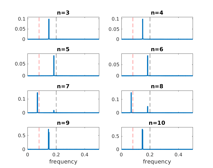
Figure 18: Power spectral density of the 3-D POD mode amplitudes 3 to 10 $|\hat{a}_{n}^{3D,M_{0}}|^{2}$ in the simplified model - the red and black lines respectively correspond to the two frequencies 0.08 and 0.2.

VI.2 Switches

We now examine if and how switches can be reproduced by a more complex version of the model, which we derive by relaxing the assumptions of the simplified model as follows:

• the second mode is allowed to vary.

• feedback is provided between the unresolved terms and the modes of the truncation.

As shown in  [21], we assume that the rate of energy transferred to the small scales depends on the energy available in the largest scales. If more energy is available in the large scales, then more energy is extracted by the small scales and conversely. This leads to us to introduce a time-varying viscosity term, so that the effect of the unresolved terms is modelled as

$$T_{n}=A_{n}a_{n}+\epsilon_{n}$$ (20)

where

1. the time-averaged value $<A_{n}>$ satisfies

   $$<A_{n}>=-L_{n}-Q_{nn1},$$ (21)

2. $A_{n}$ contains a linear part and a quadratic part

   $$A_{n}=<A_{n}>-\alpha_{n}\sum_{p=2}^{10}\lambda_{p}+\alpha_{n}\sum_{p=2}^{10}\lambda_{p}|a_{p}|^{2},$$ (22)

   As has been shown in [21], we have

   $$T_{n}=(<A_{n}>+\alpha_{n}\sum_{p\geq 1}^{N}\lambda_{p}-\alpha_{n}\sum_{p\geq 1}^{N}|a_{p}|^{2})a_{n}+\epsilon_{n}$$ (23)

   where

   $$\alpha_{n}=-\frac{<A_{n}>}{2\sum_{p\geq 2}^{N}\lambda_{p}}.$$

   The value of $\alpha_{i}$ was evaluated to be around 0.5. Since the model was not found to be largely insensitive to the exact values of $\alpha_{i}$, in what follows a constant value of $\alpha_{i}=\alpha=0.5$ was used for all modes for the sake of simplicity. Examination of equation (20) and of the POD eigenvalues shows that about 50% of the turbulent viscosity is dependent on the amplitude of mode $a_{2}$. In that sense the structure of the model displays similarities with both [22] and [3]’s model, which includes a cubic term in $a_{2}$. However it is derived from entirely different physical arguments.

3. $\epsilon_{n}$ represents Gaussian noise. The amplitude of the noise used to integrate the model was determined using $\epsilon_{n}\approx|A_{n}|$. We used $\epsilon_{2}=0.09$ and $\epsilon_{i}=0.04$ for $3\leq i\leq 10$. [A Gaussian variable was generated every $2.5$ convective time units and linearly interpolated was used for the integration].

The modified model reads:

$$\dot{a}_{1} = 0$$ (24)

$$\dot{a}_{2} = (L_{2}-\alpha\sum_{2}^{10}a_{p}^{2}\lambda_{p})a_{2}+\epsilon_{2}$$ (25)

$$\dot{a}_{3} = (L_{3}-\alpha\sum_{2}^{10}a_{p}^{2}\lambda_{p})a_{2}+0.71a_{4}+\epsilon_{3}$$ (26)

$$\dot{a}_{4} = (L_{4}-\alpha\sum_{2}^{10}a_{p}^{2}\lambda_{p})a_{2}-0.74a_{3}+\epsilon_{4}$$ (27)

$$\dot{a}_{5} = (L_{5}-\alpha\sum_{2}^{10}a_{p}^{2}\lambda_{p})a_{2}-1.09a_{6}+\epsilon_{5}$$ (28)

$$\dot{a}_{6} = (L_{6}-\alpha\sum_{2}^{10}a_{p}^{2}\lambda_{p})a_{2}-1.2a_{5}+\epsilon_{6}$$ (29)

$$\dot{a}_{7} = (L_{7}-\alpha\sum_{2}^{10}a_{p}^{2}\lambda_{p})a_{2}-0.42a_{8}+\epsilon_{7}$$ (30)

$$\dot{a}_{8} = (L_{8}-\alpha\sum_{2}^{10}a_{p}^{2}\lambda_{p})a_{2}-0.55a_{5}+0.44a_{7}+\epsilon_{8}$$ (31)

$$\dot{a}_{9} = (L_{9}-\alpha\sum_{2}^{10}a_{p}^{2}\lambda_{p})a_{2}-0.6a_{4}-0.86a_{10}+\epsilon_{9}$$ (32)

$$\dot{a}_{10} = (L_{10}-\alpha\sum_{2}^{10}a_{p}^{2}\lambda_{p})a_{2}-0.88a_{3}+0.98a_{9}+\epsilon_{10}.$$ (33)

The quadratic terms in the expression for $a_{2}$ are not included in the model as their magnitude was small (we checked that including these terms in the equations did not change the dynamics reported below).

The effect of the feedback term on the dynamics of the model is that if there is less energy in mode $a_{2}$, the higher-order modes will extract less energy, which will allow mode $a_{2}$ to grow. Conversely, if mode $a_{2}$ becomes too large, the energy transfer to the higher-order modes will be increased, which will in turn affect the energy of mode $a_{2}$.

Figures  19 and  20 shows results of the model integration for a noise amplitude of about 0.15. Figure  19 (left) shows the 3-D coefficient $a_{2}^{3d}$ predicted with the model M along with the 2-D coefficient $a_{2}^{2d}$ in the experiment, which appears a relevant comparison since, as shown in the previous section, there is a reasonably good correlation between $a_{2}$ in 3-D and 2-D (0.6). The model displays time scales of $O(1000)$ between switches, in agreement with experimental observations. Figure  19 (right) shows that the histogram of the amplitude is similar to that observed in the experiment in figure  6. This shows that the model is able to reproduce deviations in a way that is consistent with experiments. As figure  20 indicates, modes 3 to 10 are characterized by relatively fast oscillating time scales and slower amplitude variations. The frequencies of the amplitudes are shown in figure  20 (right) and compare relatively well with those measured in the simulation, given the crudeness of the truncation. Table  2 (last line) shows that the magnitude of the normalized POD amplitudes is relatively well estimated by the model with values of about 0.2 to 2 for the last modes of the truncation (we emphasize that the model contains only 20% of the total fluctuating energy). The main dynamics of the largest scales are therefore captured by the model.

n	1	2	3	4	5	6	7	8	9	10
$L_{i}$		-0.05	-0.05	-0.05	-0.05	-0.05	-0.05	-0.05	-0.05	-0.05
$<a_{n}^{2}>_{M_{0}}$	1	1	0.93	0.93	0.86	0.86	1.45	1.51	1.05	1.05
$<a_{n}^{2}>_{M}$	1	1.05	0.29	0.29	0.18	0.18	1.01	1.03	2.05	2.33

Table 2: Model linear coefficients and predicted energy

$Q_{1jm}$	m=3	m=4	m=5	m=6	m=7	m=8	m=9	m=10
j=3	0.21	0.91				-0.22		0.37
j=4	-0.94	0.23				0.0	0.29	0.17
j=5			0.22	1.09	0.	0.34
j=6			-1.22	0.20	-0.12	-0.10
j=7				0.17	0.16	-0.42
j=8			0.55		0.4	0.17
j=9	0.32		0.59				0.22	-0.86
j=10	-0.88	-0.18					0.98	0.24

Table 3: Quadratic interaction coefficients with the main mode $Q_{j1m}$; Only coefficients larger than 0.1 are indicated; only coefficients larger than 0.4 (indicated in bold) are included in the model.

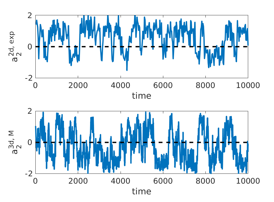
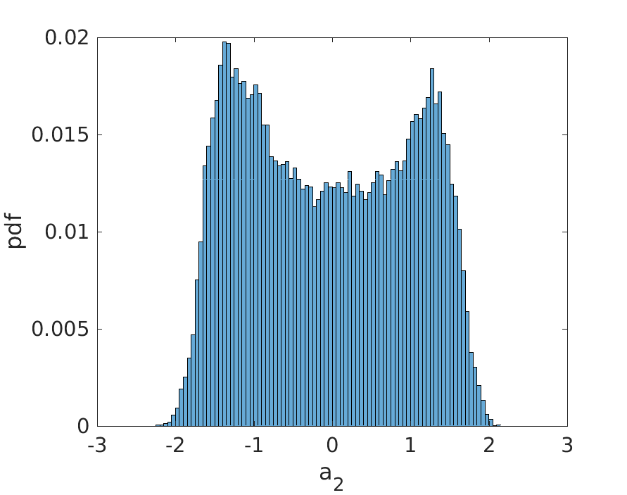
Figure 19: Left) POD amplitude $a_{2}$; top: model M (3D); bottom: experiment (2D); right) histogram of $a_{2}$

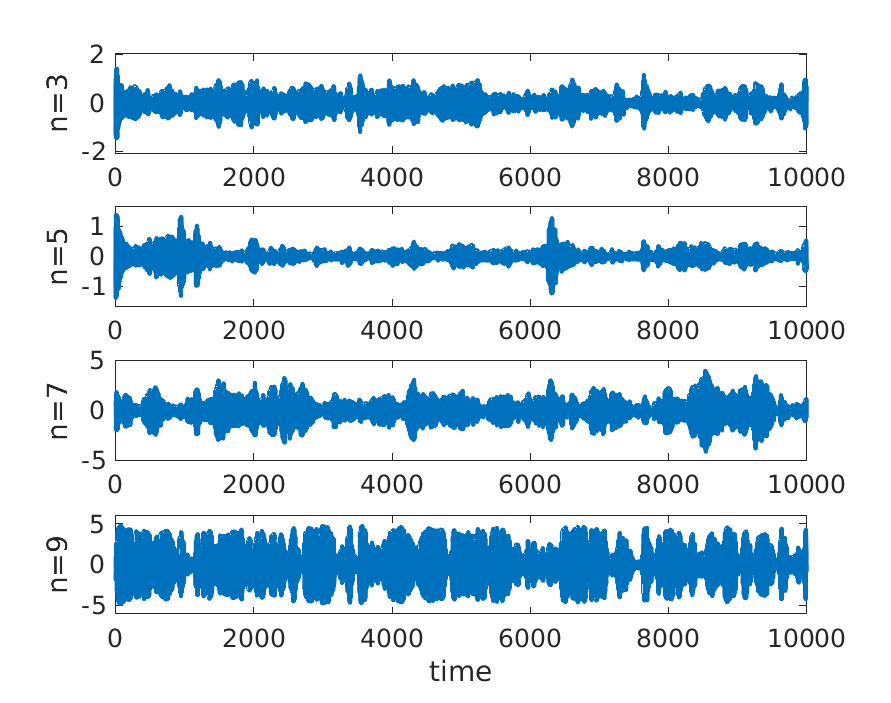
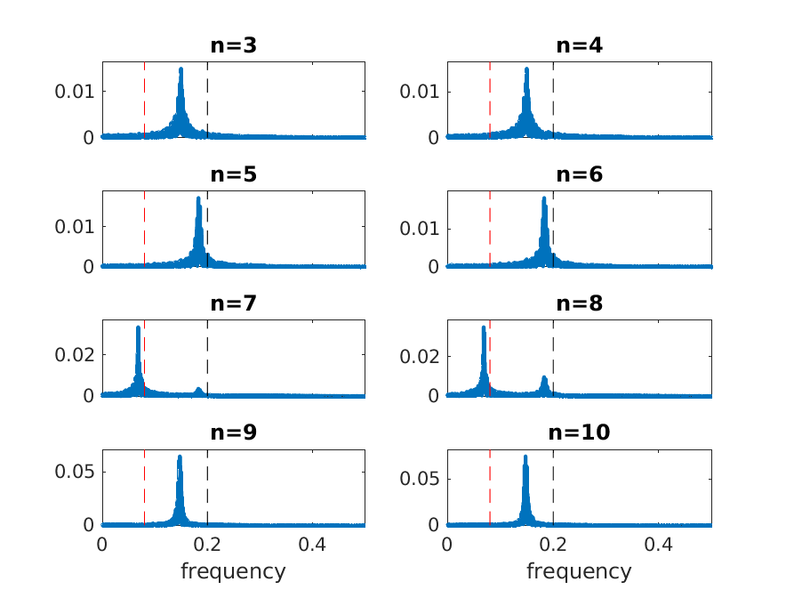
Figure 20: Left) amplitudes of 3-D POD amplitudes of modes 3, 5 , 7 and 9 in the model; right) power spectral density of POD amplitudes in the model $|\hat{a}_{n}^{3d,M}|^{2}$ - the red and black lines respectively correspond to the two frequencies 0.08 and 0.2.

VII Conclusion

We have applied Proper Orthogonal Decomposition to the 3-D numerical simulation of the flow behind an Ahmed body at $Re=10^{4}$. Reflection symmetry was applied to the computed data set in order to compensate for the relatively short time of the simulation, which precludes the observation of switches in the wake deviation. As a consequence of the enforced statistical symmetry, the flow can be decomposed into symmetric and antisymmetric structures. The mean flow consists of a symmetric recirculation bubble and an antisymmetric deviation, the effect of which is to gather flow streamlines around one of the base diagonals. 2-D POD analysis was performed in the near-wake in the simulation and compared with experimental results obtained for the same geometry. Despite the discrepancy in Reynolds number between the simulation and the experiment, an excellent agreement was observed for both the spatial structure and temporal statistics of the POD modes.

2-D results were then confronted with a 3-D approach. The energetic importance of the quasi-steady wake deviation was established. The evolution of this global 3-D deviation mode was relatively well captured by 2-D measurements in the near-wake. The next most energetic patterns are associated with vortex shedding and wake pumping. Characteristic frequencies were identified for each type of structure. Structures associated with wake pumping were characterized by a low frequency of about 0.08. Both symmetric and antisymmetric structures associated with vortex shedding in respectively the vertical and spanwise direction were characterized by dominant frequencies of 0.19 and 0.23 in the far wake. A strong negative correlation was noted between the intensity of the vortex shedding modes and the magnitude of the quasi-steady deviation. In addition, increases in the base drag were found to correspond to an increase of the quasi-steady deviation, along with a shrinkage of the recirculation zone associated with wake pumping.

Finally, POD-based low-dimensional models were derived for the largest scales of the flow. The energy content of the modes was correctly captured by the model. A simplified model was able to single out the main frequencies of the POD amplitudes observed in the simulation from the spatial modes, regardless of the time separation between the snapshots used to compute POD. This predictive ability of the model is remarkable in view of the slow convergence of the decomposition, which reflects the complexity of the flow. A more elaborate version of the model was also considered. The approach is consistent with Rigas et al.’s model [22] and in particular the structure of the model would be the same if the POD truncation was limited to two modes. By accounting for the effect of the unresolved modes with a feedback term, the POD-based model was able to reproduce the characteristics of the switches in the wake deviation. The success of the model supports the idea that wake switching is triggered by higher-order modes.

References

- [1] R.D. Brackston, J.M. Garci De La Cruz, A. Wynn, G. Rigas, and J.F. Morrison. Stochastic modelling and feedback control of bistability in a turbulent bluff bodywake. J. Fluid Mech., 802:726–749, 2016.
- [2] O. Cadot. Stochastic fluid structure interaction of three-dimensional plates facing a uniform flow. J. Fluid Mech., 794:726–749, 2016.
- [3] O. Cadot, A. Evrard, and L. Pastur. Imperfect supercritical bifurcation in a three-dimensional turbulent wake. Phys. Review E., 91(6), 2015.
- [4] L. Dalla Longa, O. Evstafyeva, and A. S. Morgans. Simulations of the bi-modal wake past three-dimensional blunt bluff bodies. Journal of Fluid Mechanics, 866:791–809, 2019.
- [5] A. Evrard, O. Cadot, V. Herbert, D. Ricot, R. Vigneron, and J. Delery. Fluid force and symmetry breaking modes of a 3d bluff body with a base cavity. Journal of Fluids and Structures, 61:99–114, 2016.
- [6] O. Evsafyeva, A. Morgans, and L. Dalla Longa. Simulation and feedback control of the ahmed body flow exhibiting symmetry breaking behaviour. J. Fluid Mech., 817, 2017.
- [7] D. Fabre, F. Auguste, and J. Magnaudet. Bifurcations and symmetry breaking in the wake of axisymmetric bodies. Phys. Fluids, 20(0517), 2017.
- [8] M. Grandemange, O. Cadot, and M. Gohlke. Reflectional symmetry breaking of the separated flow over three-dimensional bodies. Physical Review E, 86(3):035302, 2012.
- [9] M. Grandemange, M. Gohlke, and O. Cadot. Turbulent wake past a three-dimensional blunt body. part 1 - experimental sensitivity analysis. J. Fluid Mech., 752:439–461, 2013.
- [10] M. Grandemange, M. Gohlke, and O. Cadot. Turbulent wake past a three-dimensional blunt body. part 1 - global modes and bi-stability. J. Fluid Mech., 722:1–26, 2013.
- [11] P. Holmes, J.L. Lumley, and Gal Berkooz. Turbulence, Coherent Structures, Dynamical Systems and Symmetry. Cambridge University Press, 1996.
- [12] M. Kiya and Y. Abe. Turbulent elliptic wakes. J. Fluids Struct., 13:1041–1067, 1999.
- [13] R. Li, D. Barros, J. Borée, O. Cadot, B.R. Noack, and L. Cordier. Feddback control of bimodal wake dynamics. Exp Fluid, 51(4):158, 2016.
- [14] J.M. Lucas, O. Cadot, V. Herbert, S. Parpais, and J. Délery. A numerical investigation of the asymmetric wake mode of a squareback ahmed body - effect of a base cavity. J. Fluid Mech., 831:675–697, 2017.
- [15] J.L. Lumley. The structure of inhomogeneous turbulent flows. In A.M Iaglom and V.I Tatarski, editors, Atmospheric Turbulence and Radio Wave Propagation, pages 221–227. Nauka, Moscow, 1967.
- [16] R. Pasquetti and N. Peres. Simulation and feedback control of the ahmed body flow exhibiting symmetry breaking behaviour. Computers and Fluids, 114:203–217, 2015.
- [17] G. Pavia, M. Passmore, and C. Sardu. Evolution of the bi-stable wake of a square-back automotive shape. Exp. in Fluids, 59:2742, 2018.
- [18] A.K. Perry, G. Pavia, and M. Passmore. Influence of short rear end tapers on the wake of a simplified square-back vehicle: wake topology and rear drag. Experiments in Fluids, 57(11), 2016.
- [19] B. Podvin. A pod-based model for the wall layer of a turbulent channel flow. Phys. Fluids, 21(1):015111, 2009.
- [20] B. Podvin and Y. Fraigneau. A few thoughts on proper orthogonal decomposition in turbulence. Physics of FLuids, 29:020709, 2017.
- [21] B. Podvin and A. Sergent. Precursor for wind reversal in a square rayleigh-bénard cell. Phys. Rev. E, 95:013112, 2017.
- [22] G. Rigas, A.S Morgans, R.D. Brackston, and J.F. Morrison. Diffusive dynamics and stochastic models of turbulent axisymmetric wakes. J. Fluid Mech., 778(R2), 2015.
- [23] G. Rigas, A.S Morgans, and J.F. Morrison. Stability and coherent structures in the wake of axisymmetric bluff bodies. Fluid Mechanics and its Applications, 107:143–148, 2015.
- [24] G. Rigas, A.R. Oxlade, A.S Morgans, and J.F. Morrison. Low-dimensional dynamics of a turbulent axisymmetric wake. J. Fluid Mech., 755:159, 2014.
- [25] P.J. Schmid. Dynamic mode decomposition of numerical and experimental data. J. Fluid Mech., 656:5–28, 2010.
- [26] L. Sirovich. Turbulence and the dynamics of coherent structures part i: Coherent structures. Quart. Appl. Math., 45(3):561–571, 1987.
- [27] E. Varon, Y. Eulalie, S. Edwige, P. Gilotte, and J.L. Aider. Chaotic dynamics of large-scale structures in a turbulent wake. Phys. Review Fluids ., 2(034604), 2017.
- [28] R. Volpe, P. Devinant, and A. Kourta. Experimental characterization of the unsteady natural wake of the full-scale square back ahmed body: flow bi-stability and spectral analysis. Exp. in Fluids, 56(5):1–22, 2015.
- [29] E. Wassen, S. Eichinger, and F. Thiele. Simulation of active drag reduction for a square-back vehicle. Notes on Numerical Fluid Mechanics and Multidisciplinary Design, 108:241–255, 2014.