Magnetoconductance, Quantum Hall Effect, and Coulomb Blockade
in Topological Insulator Nanocones

Abstract

Magnetotransport through cylindrical topological insulator (TI) nanowires is governed by the interplay between quantum confinement and geometric (Aharonov-Bohm and Berry) phases. Here, we argue that the much broader class of TI nanowires with varying radius $\textendash$ for which a homogeneous coaxial magnetic field induces a varying Aharonov-Bohm flux that gives rise to a non-trivial mass-like potential along the wire $\textendash$ is accessible by studying its simplest member, a TI nanocone. Such nanocones allow to observe intriguing mesoscopic transport phenomena: While the conductance in a perpendicular magnetic field is quantized due to higher-order topological hinge states, it shows resonant transmission through Dirac Landau levels in a coaxial magnetic field. Furthermore, it may act as a quantum magnetic bottle, confining surface Dirac electrons and leading to a largely interaction-dominated regime of Coulomb blockade type. We show numerically that the above-mentioned effects occur for experimentally accessible values of system size and magnetic field, suggesting that TI nanocone junctions may serve as building blocks for Dirac electron optics setups.

Electronic transport across phase-coherent structures has been a central topic of solid state research ever since the birth of mesoscopic physics some 40 years ago. While the complexity of mesoscopic setups has steadily increased, from the simple gate-defined quantum point contacts of the ’80s van Wees et al. (1988) to elaborate present-day electron optics circuits in semiconductors Bocquillon et al. (2013) and graphene Kumada et al. (2016); Makk et al. (2018), their structure remains in the vast majority of cases planar – i.e. transport takes place in flat two-dimensional (2D) space. Exceptions to the 2D scenario are samples based on carbon nanotubes and 3D topological insulator (3DTI) nanowires Peng et al. (2009); Dufouleur et al. (2013); Cho et al. (2015); Ziegler et al. (2018). 3DTIs are bulk band insulators hosting protected 2D surface metallic states à la Dirac Hasan and Kane (2010). In mesoscopic nanostructures built out of 3DTIs low-temperature phase-coherent transport takes place on a 2D Dirac metal wrapped around an insulating 3D bulk. As such, it is strongly dependent on a peculiar conjunction of structural (real space) and spectral (reciprocal space) geometrical properties. This has remarkable consequences for a topological insulator nanowire (TINW) with constant circular cross section in a coaxial magnetic field, shown in Fig. 2(a). Its magnetoconductance reflects a non-trivial interplay between two fundamentals of mesoscopic physics: quantum confinement and geometric [Aharonov-Bohm (AB) and Berry] phases Ostrovsky et al. (2010); Bardarson et al. (2010); Dufouleur et al. (2013); Cho et al. (2015); Ziegler et al. (2018); Dufouleur et al. (2018).

An interesting twist offered by 3DTIs is the possibility of engineering shaped TINWs with a variable cross section, e.g. truncated TI nanocones (TINCs) as sketched in Fig. 1(a). When a coaxial magnetic field is switched on, shaped TINWs possess the unique feature that surface charge carriers traversing the wire, experience not only a variation of the centrifugal potential, but also a spatially changing AB flux – a property that cannot easily be realized with bulk conductors. This gives rise to a flux-dependent effective mass potential along the TINC, which induces a variety of interesting mesoscopic transport phenomena, including resonant transport through Dirac Landau levels and magnetically induced Coulomb blockade physics. Due to the non-trivial real space geometry, all such transport regimes can be accessed simply by applying and tuning a homogeneous magnetic field.

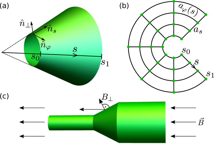
Figure 1: (a) Sketch of a TINC extended to its conical singularity with local coordinate vectors $\hat{n}_{\varphi},\hat{n}_{s},\hat{n}_{\perp}$. (b) Unfolded cone grid used for numerical simulations. (c) TINC in coaxial B-field (with $B_{\perp}=\bm{B}\cdot\hat{n}_{\perp}$) with cylindrical leads attached.

Cylindrical TINW in a magnetic field – For later reference consider cylindrical TINWs of radius $R$ in coaxial Ostrovsky et al. (2010); Bardarson et al. (2010); Dufouleur et al. (2013); Cho et al. (2015); Ziegler et al. (2018); Dufouleur et al. (2018) or perpendicular Ajiki and Ando (1993); Vafek (2011); Zhang et al. (2012); Sitte et al. (2012); Brey and Fertig (2014); de Juan et al. (2014); König et al. (2014); Xypakis and Bardarson (2017) magnetic fields. They can be described by the 2D surface Dirac Hamiltonian Zhang and Vishwanath (2010) ${H}\!=\!v_{F}\left[\frac{1}{2}\left({p}_{\varphi}\sigma_{\varphi}+\sigma_{\varphi}{p}_{\varphi}\right)+\sigma_{z}{p}_{z}\right]$ with Fermi velocity $v_{F}$, coordinate along the wire axis $z$, and azimuthal angle $\varphi$. Furthermore, $p_{\varphi}\!=\!\frac{-i\hbar}{R}\partial_{\varphi}$ and $\sigma_{\varphi}\!=\!\sigma_{y}\cos\varphi-\sigma_{x}\sin\varphi$ with Pauli matrices $\sigma_{x}$, $\sigma_{y}$, $\sigma_{z}$. The unitary transformation $U\!=\!\exp(i\sigma_{z}\varphi/2)$ yields $H=v_{F}\left(\sigma_{y}p_{\varphi}+\sigma_{z}p_{z}\right)$ and antiperiodic boundary conditions for the wave functions. The associated Berry phase Mikitik and Sharlai (1999) shifts the angular momentum quantization condition by $\hbar/2$, yielding a gapped subband spectrum $E_{l}(p_{z})\!=\!\pm v_{F}\sqrt{p_{z}^{2}+\hbar^{2}(l+1/2)^{2}/R^{2}}$, with orbital angular momentum quantum number $l\in\mathbb{Z}$.

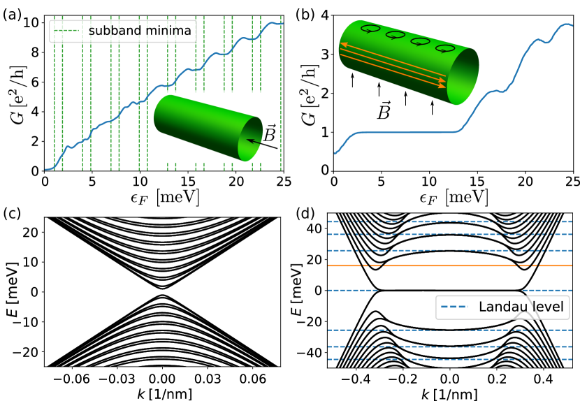
Figure 2: Disorder-averaged conductance as function of the Fermi energy $\epsilon_{F}$ (top panels) and band structure (with longitudinal wave number $k$, bottom) of a cylindrical TI nanowire in a coaxial (left) and perpendicular (right) magnetic field $B\!=\!2\,$T. The orange arrows in (b) sketch 1D hinge states at an energy marked with an orange line in (d). Wire size: length $L\!=\!600\,$nm, circumference $C\!=\!700\,$nm. We use a Gaussian-correlated disorder average taken over 600 configurations, and a Fermi velocity of $v_{F}=$5\text{\times}{10}^{5}\text{\,}\mathrm{m}\mathrm{/}\mathrm{s}$$ here and throughout.

For a coaxial $B$-field generating a magnetic flux $\Phi\!=\!\pi R^{2}B$ ($B\!=\!|\bf B|$) through the tube the problem remains separable and reduces to that of an electron in an AB ring – the cylinder cross section – times free longitudinal motion. The discrete spectrum of the ring is periodic in $\Phi_{0}$ Eckern and Schwab (1995), and is turned into a series of 1D subbands by free longitudinal motion. Due to the Berry phase the bands are gapped for $\Phi\!=\!n\Phi_{0}$ and gapless for $\Phi\!=\!(n+1/2)\Phi_{0},n\in\mathbb{Z}$ Ostrovsky et al. (2010); Bardarson et al. (2010). Figure 2(c) shows the generic situation with $\Phi\approx 18.86\,\Phi_{0}$. The corresponding conductance is depicted in Fig. 2(a), increasing with energy as more channels open Ziegler et al. (2018). For details of the numerics see below and the Supp. Mat. Sup .

If the magnetic field is orthogonal to the nanowire axis, the situation changes drastically. The resulting band structure, see Fig. 2(d), can be understood qualitatively in classical terms Onorato (2011): The field component $B_{\perp}=B\cos\varphi$ perpendicular to the surface varies along the wire circumference, being maximal for $\varphi\!=\!0,\pi$ (cylinder top and bottom) and zero for $\varphi\!=\!\pi/2,\,3\pi/2$ (sides), where its sign changes. Cyclotron orbits [black circles in Fig. 2(b)] of opposite handedness thus form on the top and bottom surfaces, while “snaking” orbits propagating along the sides appear (orange arrows). Quantum mechanically, the former lead to Landau level (LL) formation, while the latter are chiral 1D hinge states crossing the $B_{\perp}$-induced gap and signaling a higher-order TI phase . The dashed lines in Fig. 2(d) mark the LL energies for $B=B_{\perp}(\varphi=0)$,

$$E_{n}=\mathrm{sgn}(n)\frac{\hbar v_{F}}{l_{B}}\sqrt{2|n|}\;,\;n\in\mathbb{Z}\,,$$ (1)

where $l_{B}=\sqrt{\hbar/(eB)}$ is the magnetic length. Around $k\!=\!0$, flat bands represent well-formed LLs. The upward (downward) bending $n\!=\!0$ subband ensures the existence of a robust conductance plateau $G\!=\!e^{2}/h$ in a large energy window, see Fig. 2(b), where only one chiral hinge state per side is present, preventing backscattering. The dip at $\epsilon_{F}=0$ is treated in Ref. Xypakis and Bardarson (2017).

TINC in a coaxial magnetic field – We generalize our considerations to a TINC, see Fig. 1(a), a representative building block of TINWs with varying cross section. We parametrize its surface by the azimuthal angle $\varphi$ and the distance $s$ to the conical singularity. The radius is $R(s)\!=\!s\,\sin(\beta/2)$, $\beta$ denoting the cone opening angle and $s_{0}\!\!\leq s\!\leq s_{1}$. Using standard techniques Xypakis et al. (2017) and after the unitary transformation $U\!=\!\exp(i\sigma_{z}\varphi/2)$, the surface Dirac Hamiltonian reads

$${H}=v_{F}\left[\left({p}_{s}-\frac{i\hbar}{2s}\right)\sigma_{z}+{p}_{\varphi}(s)\sigma_{y}\right]\,,$$ (2)

with ${p}_{\varphi}(s)\!=\!-\frac{i\hbar}{R(s)}\partial_{\varphi}$. The spin connection term $-\frac{i\hbar}{2s}$ Fecko (2006) makes it Hermitian with respect to the scalar product

$$\left<\Psi_{1}|\Psi_{2}\right>\equiv\int_{s_{0}}^{s_{1}}\!\mathrm{d}s\int_{0}^{2\pi}\!\mathrm{d}\varphi\;R(s)\Psi_{1}^{*}(s,\varphi)\Psi_{2}(s,\varphi)\,.$$ (3)

Transforming $\Psi\rightarrow\widetilde{\Psi}\!=\!\sqrt{R(s)}\Psi$ and $H\rightarrow\tilde{H}\!=\!\sqrt{R(s)}H(1/\sqrt{R(s)})$ removes the spin connection term from Eq. (2) and renders the volume form $R(s){\rm d}\varphi{\rm d}s$ trivial. This yields

$${\tilde{H}}=v_{F}[p_{s}\sigma_{z}+p_{\varphi}(s)\sigma_{y}]\,,$$ (4)

with $\langle\widetilde{\Psi}_{1}|\widetilde{\Psi}_{2}\rangle\!\equiv\!\int\!\mathrm{d}s\int\!\mathrm{d}\varphi\widetilde{\Psi}_{1}^{*}(s,\varphi)\widetilde{\Psi}_{2}(s,\varphi)$, which is necessary for our numerics Sup .

In presence of a coaxial magnetic field the problem remains rotationally symmetric and thus separable. We proceed via the exact separation ansatz $\widetilde{\Psi}_{nl}(s,\varphi)\!=\!\mathrm{e}^{i(l+1/2)\varphi}\chi_{nl}(s)$, with $\chi_{nl}(s)$ a two-component spinor. The +1/2 in the exponential originates from the curvature-induced Berry phase, $l$ is the orbital angular momentum quantum number, and the meaning of $n$ will be clarified shortly. Using minimal coupling $p_{\varphi}(s)\rightarrow p_{\varphi}(s)\!+\!eA_{\varphi}(s)$ yields the 1D Dirac equation

$$\left[v_{F}{p}_{s}\sigma_{z}+V_{l}(s,B)\sigma_{y}\right]\chi_{nl}(s)=\epsilon_{nl}\chi_{nl}(s).$$ (5)

Here, the angular momentum term

$$V_{l}(s,B)=\frac{v_{F}\hbar}{R(s)}\left(l+\frac{1}{2}-\frac{\Phi(s,B)}{\Phi_{0}}\right),$$ (6)

with $\Phi(s,B)\!=\!\pi R^{2}(s)B$, acts as a position-dependent mass potential, and is crucial for predicting the TINC magnetotransport properties – indeed, more generally the properties of arbitrarily shaped, rotationally symmetric TINWs to_ . Its mass-like character becomes evident in Eq. (5), where it couples to $\sigma_{y}$, while a simple electrostatic potential enters the equation with the identity matrix. Hence, Eq. (5) describes 1D Dirac electrons feeling the effective potential $|V_{l}(s)|$. Dirac electrons Klein-tunnel through electrostatic barriers, but not through $|V_{l}(s)|$. Figure 3(b) shows $|V_{l}(s,B)|$ for a coaxial $B$-field, whose $B_{\perp}$ yields $l_{B}\ll s_{1}-s_{0}$ for all $l$-values relevant in the presented energy range (only $l=15$ and $l=25$ are colored and labeled, the rest is gray). In transport, an electron injected in mode $l$ feels a distinct effective potential $|V_{l}(s,B)|$. For a discussion of the $B$-field dependence of $|V_{l}(s,B)|$ and the formation of wedges shown in Fig. 3(b) see Sup . Note that due to the step-like form of $B_{\perp}(s)$, cf. Fig. 1(c), the situation is similar to single-valley graphene subject to a magnetic barrier De Martino et al. (2007); Ramezani Masir et al. (2008).

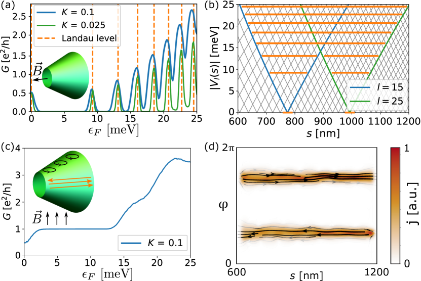
Figure 3: Disorder averaged TI nanocone conductance for coaxial and perpendicular magnetic field. (a) Coaxial field: resonant transmission through LLs. Stronger disorder (larger $K$ Sup ) broadens and shifts the LLs from their unperturbed positions marked by vertical dashed lines Peres et al. (2006); Dóra (2008). (b) LL formation in effective wedge potentials. (c) Perpendicular field: robust conductance plateau due to topologically protected chiral hinge states and associated current density in (d). Parameters: $B\!=\!2\,$T; cone with (arc) length $600\,$nm and opening angle $\beta\!=\!15^{\circ}$, beginning a distance $s_{0}\!=\!600\,$nm away from the conical singularity, yielding minimal and maximal circumferences $C_{\rm min}\!\approx\!492\,$nm, $C_{\rm max}\!\approx\!984\,$nm (see Fig. 1).

Magnetotransport through TINCs – Our quantum transport simulations including disorder are based on the software package kwant Groth et al. (2014). The tight-binding representation of Eq. (2) is non-Hermitian due to the non-trivial volume form Sup . The latter is rendered trivial by the transformation ${H}\rightarrow{\tilde{H}}$, hence Eq. (4) has a Hermitian tight-binding representation. Conventional discretization of Eq. (4) leads to the effective lattice shown in Fig. 1(b), representing the unfolded cone. The transversal lattice constant $a_{\varphi}(s)$, which is part of the hopping integral, is adapted such that $N_{\varphi}a_{\varphi}(s)\!=\!U(s)$, where $N_{\varphi}$ is the number of lattice points and $U(s)$ the circumference at position $s$, and the ends are “glued” together (for details see Sup ). To compute the conductance, highly-doped semi-infinite cylindrical leads with radii $R(s_{0})$ and $R(s_{1})$ are attached to the conical scattering region, see Fig. 1(c).

Figure 3(a) shows the TINC conductance for the potential $|V_{l}(s,B)|$ in Fig. 3(b). Sharp peaks signal resonant transmission through quasi-bound states of wedge-shaped effective potentials: Each wedge (labeled by $l$) hosts a sequence of bound states (labeled by $n$) whose energies $\left\{\epsilon_{nl}\right\}$, marked by horizontal orange lines in Fig. 3(b), are solutions of Eq. (5). The latter are quantum Hall (QH) states, degenerate in $l$ and forming the Dirac LL given in Eq. (1). The LL degeneracy is thus given by the number of wedges within the cone (between $s_{0}$ and $s_{1}$). In a clean TINC degenerate states in adjacent wedges are orthogonal, hence transport is exponentially suppressed. Disorder breaks rotational symmetry and couples adjacent states leading to broadened resonant tunneling peaks, see Fig. 3(a). Indeed, stronger disorder increases the coupling between QH states, and thus the conductance (compare green and blue curves). Note the close relation to a QH Corbino geometry Rycerz (2010): Looking at the TINC from the front, its 2D projection is a ring of finite thickness in a homogeneous perpendicular magnetic field $B_{\perp}$.

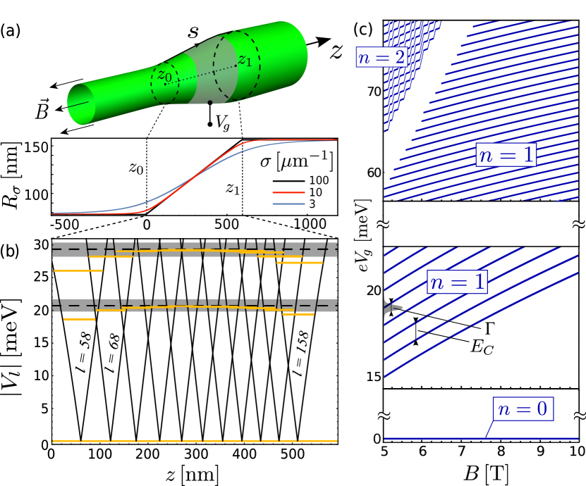
Figure 4: Anomalous Coulomb blockade in TI nanocones. (a) Smoothed TINC parametrized by $R_{\sigma}(z)$ Sup with $\sigma\!=\!10\,\mu$m^-1 (small $\sigma$ corresponds to strong smoothing, see lower panel). A gate wrapping around the TINC is sketched by the gray region. (b) $|V_{l}(z)|$ from $l\!=\!58$ to $l\!=\!158$ (in steps of $\Delta l\!=\!10$) are shown for $B\!=\!10\,$T. QH states (marked by orange lines) with $n\!\neq\!0$ are no longer resonant across the entire junction, leading to tunnel barriers close to $z_{0},z_{1}$. Grey shade depicts the disorder broadening $\Gamma$ from Fig. 3(a) for $K=0.1$. (c) Addition spectrum of the $n=0,1,2$ LLs in the central TINC region, with charging energy $E_{C}\!=\!1\,$meV. The $n=1,2$ LLs, defined by QH states whose energy lies within the disorder broadening, are Coulomb split by $E_{C}$, while $n=0$ QH states are not affected by Coulomb repulsion.

For a TINC in a $B$-field orthogonal to its symmetry axis, the conductance is completely different, see Fig. 3(c). Its main features – dip at zero energy, plateau up to $E\!\simeq\!13\,{\rm meV}$ and subsequent disorder-smoothed steps – stem from second-order topological hinge states at the sides. If $l_{B}\!\ll\!\pi R(s_{0})$, they are indistinguishable from those of a cylindrical TINW, cf. Figs. 2(b) and 3(c). This is actually true in a much more general sense: As long as top and bottom surface provide enough space for LLs to form, the geometry of the TINW in perpendicular B-field is irrelevant for the qualitative conductance features, as opposed to TINWs in coaxial B-field. The current density associated with the lowest-energy hinge state of the TINC, yielding the robust plateau, is plotted in Fig. 3(d) and seen to be chiral – the current on opposite sides $(\varphi\!=\!\pi/2,3\pi/2)$ flows in opposite directions.

The two settings in Fig. 3(a) and (c) correspond to a longitudinal ($\sigma_{xx}$) and transversal ($\sigma_{xy}$) conductivity measurement in a conventional 2D QH setup where the longitudinal current density reads $j_{x}\!=\!\sigma_{xx}E_{x}\!+\!\sigma_{xy}E_{y}$. Let us adapt this to the TINC. In a perpendicular magnetic field, $E_{x}$ vanishes as long as $\epsilon_{F}$ lies within the plateau due to lack of backscattering. Hence, the conductance is solely determined by $\sigma_{xy}$. On the contrary, in a coaxial magnetic field $E_{y}$ vanishes since metallic states extend across the circumference, resulting in a conductance determined by $\sigma_{xx}$ only.

Coulomb blockade in smoothed TINCs – Equation (5) and thus the concept of an effective potential, Eq. (6), is valid more generally for any rotationally symmetric but arbitrarily shaped TINWs, the coordinate $s$ generalizing to an arc length coordinate to_ . Exploiting the effective potential, one can devise different wire geometries featuring (tunable) magnetic barriers able to confine Dirac electrons to_ . As a simple and paradigmatic example, we consider a smoother, more realistically shaped TINC, see Fig. 4(a). In the regions of smaller slope (close to the leads) $B_{\perp}$ decreases to zero, ergo the QH states drop in energy and are no longer resonant with those in the center: a QH island representing a quantum magnetic bottle emerges in the central TINC region between magnetic tunnel barriers close to the leads.

To confirm the above qualitative statements numerically, we consider the setup of Fig. 4(a). For convenience we work with the coaxial coordinate $z$ instead of $s$. The radius $R_{\sigma}(z)$ is now characterized by a smoothing parameter $\sigma$ introducing surface curvature, ${\rm d}^{2}R_{\sigma}/{\rm d}z^{2}\neq 0$. The ideal TINC from Fig. 3 is recovered for $\sigma\to\infty$ Sup , see Fig. 4(a). Orange lines in Fig. 4(b) mark the bound state energies of the potential wedges $|V_{l}(z)|$, obtained by solving the generalized version of Eq. (5). QH states with $n\!>\!0$ close to the leads are strongly lowered in energy as compared to the central ones, which still form the (disorder-broadened) LLs expected in the limit $\sigma\!\rightarrow\!\infty$. Effective magnetic confinement requires the smooth TINC border region to be larger than the (local) magnetic length $l_{B}$, so that off-resonant QH states can form, corresponding to $B$-field strengths of order 5-10 T for the smooth TINC considered. Larger TINCs or smoother border regions allow for weaker magnetic fields. Notably, the $n\!=\!0$ LL is unaffected by the magnetic flux modulation, a distinct feature of Dirac electrons. This leads to an anomalous coexistence of transport mechanisms: $n=0$ electrons stay delocalized and the associated conductance resonant, while potential barriers close to $z_{0}$, $z_{1}$ confine $n\neq 0$ electrons, whose transport properties are then dominated by Coulomb repulsion. Indeed, when the Fermi energy aligns with an $n\neq 0$ LL, oscillations of Coulomb blockade type Beenakker (1991) should be observed by varying the gate voltage $V_{g}$ applied to the central TINC region.

An exact description of blockade oscillations in strong magnetic fields is a highly non-trivial many-body problem that, in the case of semiconductors, is often solved self-consistently Meirav and Foxman (1996). However, the general features of the addition spectrum can usually be obtained from the constant interaction model, characterized by a constant charging energy $E_{C}$, and the single-particle spectrum of the island Meirav and Foxman (1996). Hence, we stay within such a model and discuss the expected consequences. Figure 4(c) shows the addition spectrum of the inner LLs as function of $B$ assuming homogeneous gating and $E_{C}\!=\!1\,$meV (this value is justified below). The $n=0$ LL is open to the leads and thus not split by interaction effects. Conductance peaks belonging to the $n=1$ LL are constantly spaced in gate voltage. The large gap in the upper panel is the Landau gap between the first and second LLs. For increasing $B$, additional QH states join the $n=1$ LL, adding to its degeneracy and shifting upwards the bottom of the $n=2$ LL in steps of $E_{C}$. If the coupling $\Gamma_{n}^{l,r}$ to the left $(l)$ and right $(r)$ leads is roughly the same for all QH states within the n-th LL, one expects conductance peaks $G_{n}\propto\Gamma_{n}^{l}\Gamma_{n}^{r}/(\Gamma_{n}^{l}+\Gamma_{n}^{r})$ Beenakker (1991) . Besides the anomalous $n\!=\!0$ conductance peak, further differences between standard Coulomb blockade Meirav and Foxman (1996) and the present scenario are evident: First, the blockade conductance is determined by the Dirac spectrum $\propto\sqrt{B}$, not the one $\propto B$ of trivial electrons; Second, the island-lead coupling – and thus the conductance peaks height and shape – is determined by the tunable magnetic barrier $\Gamma_{n}^{l,r}(B)$. Its precise characterization is a non-trivial, setup-dependent problem. Finally, the $n\neq 0$ islands are neither featureless resonant levels as in the simple quantum dots, nor do they host QH edge states running along their perimeter Meirav and Foxman (1996). In fact, transport across each island is akin to that through a peculiar disordered system whose transmission increases with increasing disorder [see Fig. 3(b)]. Thus, our setting might host a competition between magnetically-induced blockade physics and a suitable generalization of (longitudinal) magnetotransport physics for 2D, disordered systems Dmitriev et al. (2012); Schirmacher et al. (2015), which is unexplored ground. Its study appears as a very interesting problem, albeit clearly beyond the scope of this work.

Experimental realization – The parameters used are within experimental reach: HgTe-based 3DTI tubes Ziegler et al. (2018) or core-shell nanowires Kessel et al. (2017) with spatially varying cross sections have already been built for transport experiments. Crucially, our conclusions do not require the TINC to have a truly circular cross section: Surface deformations lift the degeneracies of the QH states within each LL, but as long as this splitting is smaller than the broadening due to, e.g. temperature or disorder, no qualitative conductance change is expected. Moreover, the leads are not required to have a cylindrical shape. To achieve our results, it is merely important that there are enough lead modes available that couple to the states on the TINC. The charging energy $E_{C}$ depends on the setup size, geometry and materials, including the dielectrics, and can thus be tuned in a broad range. For a HgTe-based TINC with parameters from Ref. Ziegler et al. (2018), $E_{C}$ is of the order of $1\,$meV. Homogeneous gating can be achieved with established techniques Storm et al. (2012); Royo et al. (2017).

Conclusions – Shaped TINWs represent a broad class of mesoscopic junctions realizable with current technology which allow to explore radically different magnetotransport regimes. The latter result from the interplay between magnetic confinement of Dirac electrons, disorder and interactions. They are all accessible in TINCs by tuning a homogeneous magnetic field, and orienting it in space. TINCs and junctions thereof could act as building blocks of more complex 3D mesoscopic Dirac electron setups, where, e.g., exotic aspects of QH physics on curved surfaces can be studied Lee (2009); Can et al. (2016), or of TI-superconducting systems where Majoranas are looked for Hasan and Kane (2010); Cook and Franz (2011); Manousakis et al. (2017).

Acknowledgements – We thank Andrea Donarini, Benjamin Geiger, Milena Grifoni, Dmitry Polyakov, and Alex Kamenev for useful discussions. This work was funded by the Deutsche Forschungsgemeinschaft (DFG, German Research Foundation) – Project-ID 314695032 – SFB 1277 (project A07 and B07), and within Priority Programme SPP 1666 “Topological Insulators” (project Ri681-12/2). Support by the Elitenetzwerk Bayern Doktorandenkolleg “Topological Insulators” is also acknowledged.

References

- van Wees et al. (1988) B. J. van Wees, H. van Houten, C. W. J. Beenakker, J. G. Williamson, L. P. Kouwenhoven, D. van der Marel, and C. T. Foxon, “Quantized conductance of point contacts in a two-dimensional electron gas,” Phys. Rev. Lett. 60, 848–850 (1988).
- Bocquillon et al. (2013) E. Bocquillon, V. Freulon, F. D. Parmentier, J.-M. Berroir, B. Plaçais, C. Wahl, J. Rech, T. Jonckheere, T. Martin, C. Grenier, D. Ferraro, P. Degiovanni, and G. Fève, “Electron quantum optics in ballistic chiral conductors,” Ann. Phys. (Berlin) 526, 1 (2013).
- Kumada et al. (2016) N. Kumada, F. D. Parmentier, H. Hibino, D. C. Glattli, and P. Roulleau, “Shot noise generated by graphene p–n junctions in the quantum Hall effect regime,” Nat. Commun. 6, 8068 (2015).
- Makk et al. (2018) P. Makk, C. Handschin, E. Tóvári, K. Watanabe, T. Taniguchi, K. Richter, M.-H. Liu, and C. Schönenberger, “Coexistence of classical snake states and Aharonov-Bohm oscillations along graphene junctions,” Phys. Rev. B 98, 035413 (2018).
- Peng et al. (2009) H. Peng, K. Lai, D. Kong, S. Meister, Y. Chen, X.-L. Qi, S.-C. Zhang, Z.-X. Shen, and Y. Cui, “Aharonov-Bohm interference in topological insulator nanoribbons,” Nat. Mater. 9, 225 (2009).
- Dufouleur et al. (2013) J. Dufouleur, L. Veyrat, A. Teichgräber, S. Neuhaus, C. Nowka, S. Hampel, J. Cayssol, J. Schumann, B. Eichler, O. G. Schmidt, B. Büchner, and R. Giraud, “Quasiballistic Transport of Dirac Fermions in a Nanowire,” Phys. Rev. Lett. 110, 186806 (2013).
- Cho et al. (2015) S. Cho, B. Dellabetta, R. Zhong, J. Schneeloch, T. Liu, G. Gu, M. J. Gilbert, and N. Mason, “Aharonov-Bohm oscillations in a quasi-ballistic three-dimensional topological insulator nanowire,” Nat. Commun. 6, 7634 (2015).
- Ziegler et al. (2018) J. Ziegler, R. Kozlovsky, C. Gorini, M.-H. Liu, S. Weishäupl, H. Maier, R. Fischer, D. A. Kozlov, Z. D. Kvon, N. Mikhailov, S. A. Dvoretsky, K. Richter, and D. Weiss, “Probing spin helical surface states in topological HgTe nanowires,” Phys. Rev. B 97, 035157 (2018).
- Hasan and Kane (2010) M. Z. Hasan and C. L. Kane, “Topological Insulators,” Rev. Mod. Phys. 82, 3045 (2010).
- Ostrovsky et al. (2010) P. M. Ostrovsky, I. V. Gornyi, and A. D. Mirlin, “Interaction-Induced Criticality in Topological Insulators,” Phys. Rev. Lett. 105, 036803 (2010).
- Bardarson et al. (2010) J. H. Bardarson, P. W. Brouwer, and J. E. Moore, “Aharonov-Bohm Oscillations in Disordered Topological Insulator Nanowires,” Phys. Rev. Lett. 105, 156803 (2010).
- Dufouleur et al. (2018) J. Dufouleur, E. Xypakis, B. Büchner, R. Giraud, and J. H. Bardarson, “Suppression of scattering in quantum confined 2D helical Dirac systems,” Phys. Rev. B 97, 075401 (2018).
- Ajiki and Ando (1993) H. Ajiki and T. Ando, “Electronic states of carbon nanotubes,” J. Phys. Soc. Jpn. 62, 1255–1266 (1993).
- Vafek (2011) O. Vafek, “Quantum hall effect in a singly and doubly connected three-dimensional topological insulator,” Phys. Rev. B 84, 245417 (2011).
- Zhang et al. (2012) Y.-Y. Zhang, X.-R. Wang, and X C Xie, “Three-dimensional topological insulator in a magnetic field: chiral side surface states and quantized Hall conductance,” J. Phys. Condens. Matter 24, 015004 (2012), 1103.3761 .
- Sitte et al. (2012) M. Sitte, A. Rosch, E. Altman, and L. Fritz, “Topological insulators in magnetic fields: quantum Hall effect and edge channels with a nonquantized term.” Phys. Rev. Lett. 108, 126807 (2012).
- Brey and Fertig (2014) L. Brey and H. A. Fertig, “Electronic states of wires and slabs of topological insulators: Quantum hall effects and edge transport,” Phys. Rev. B 89, 085305 (2014).
- de Juan et al. (2014) F. de Juan, R. Ilan, and J. H. Bardarson, “Robust Transport Signatures of Topological Superconductivity in Topological Insulator Nanowires,” Phys. Rev. Lett. 113, 107003 (2014).
- König et al. (2014) E. J. König, P. M. Ostrovsky, I. V. Protopopov, I. V. Gornyi, I. S. Burmistrov, and A. D. Mirlin, “Half-integer quantum Hall effect of disordered Dirac fermions at a topological insulator surface,” Phys. Rev. B 90, 165435 (2014).
- Xypakis and Bardarson (2017) E. Xypakis and J. H. Bardarson, “Conductance fluctuations and disorder induced = 0 quantum Hall plateau in topological insulator nanowires,” Phys. Rev. B 95, 35415 (2017).
- Zhang and Vishwanath (2010) Y. Zhang and A. Vishwanath, “Anomalous Aharonov-Bohm Conductance Oscillations from Topological Insulator Surface States,” Phys. Rev. Lett. 105, 206601 (2010).
- Mikitik and Sharlai (1999) G. P. Mikitik and Yu. V. Sharlai, “Manifestation of Berry’s Phase in Metal Physics,” Phys. Rev. Lett. 82, 2147 (1999).
- Eckern and Schwab (1995) U. Eckern and P. Schwab, “Normal persistent currents,” Adv. Phys. 44, 387 (1995).
- (24) See Supplemental material.
- Onorato (2011) P. Onorato, “Landau levels and edge states in carbon nanotubes: A semiclassical approach,” Phys. Rev. B 84, 233403 (2011).
- Note (1) See Schindler et al. (2018). More precisely, we deal here with a second-order TI phase due to the applied magnetic field, and thus extrinsic Sitte et al. (2012), as opposed to intrinsic higher-order phases arising from crystal symmetries Geier et al. (2018).
- Fecko (2006) M. Fecko, “Differential geometry and lie groups for physicists,” Cambridge university press (2006) .
- (28) R. Kozlovsky et al., to be published.
- De Martino et al. (2007) A. De Martino, L. Dell’Anna, and R. Egger, “Magnetic Confinement of Massless Dirac Fermions in Graphene,” Phys. Rev. Lett. 98, 066802 (2007).
- Ramezani Masir et al. (2008) M. Ramezani Masir, P. Vasilopoulos, A. Matulis, and F. M. Peeters, “Direction-dependent tunneling through nanostructured magnetic barriers in graphene,” Phys. Rev. B 77, 235443 (2008).
- Peres et al. (2006) N. M. R. Peres, F. Guinea, and A. H. Castro Neto, “Electronic properties of disordered two-dimensional carbon,” Phys. Rev. B 73, 125411 (2006).
- Dóra (2008) B. Dóra, “Disorder effect on the density of states in Landau quantized graphene,” Low Temp. Phys. 34, 801–804 (2008).
- Groth et al. (2014) C. W. Groth, M. Wimmer, A. R. Akhmerov, and X. Waintal, “Kwant: A software package for quantum transport,” New J. Phys. 16, 063065 (2014).
- Rycerz (2010) A. Rycerz, “Magnetoconductance of the Corbino disk in graphene,” Phys. Rev. B 81, 121404(R) (2010).
- Beenakker (1991) C. W. J. Beenakker, “Theory of Coulomb-blockade oscillations in the conductance of a quantum dot,” Phys. Rev. B 44, 1646–1656 (1991).
- Meirav and Foxman (1996) U. Meirav and E. B. Foxman, “Single-electron phenomena in semiconductors,” Semicond. Sci. Technol. 11, 255–284 (1996).
- Schirmacher et al. (2015) W. Schirmacher, B. Fuchs, F. Höfling, and T. Franosch, “Anomalous magnetotransport in disordered structures: Classical edge-state percolation,” Phys. Rev. Lett. 115, 240602 (2015).
- Dmitriev et al. (2012) I. A. Dmitriev, A. D. Mirlin, D. G. Polyakov, and M. A. Zudov, “Nonequilibrium phenomena in high landau levels,” Rev. Mod. Phys. 84, 1709–1763 (2012).
- Kessel et al. (2017) M. Kessel, J. Hajer, G. Karczewski, C. Schumacher, C. Brüne, H. Buhmann, and L. W. Molenkamp, “CdTe-HgTe core-shell nanowire growth controlled by RHEED,” Phys. Rev. Materials 1, 023401 (2017).
- Storm et al. (2012) K. Storm, G. Nylund, L. Samuelson, and A. P. Micolich, “Realizing Lateral Wrap-Gated Nanowire FETs: Controlling Gate Length with Chemistry Rather than Lithography,” Nano Lett. 12, 1 (2012).
- Royo et al. (2017) M. Royo, M. De Luca, R. Rurali, and I. Zardo, “A review on III-V core- multishell nanowires: Growth, properties, and applications,” J. Phys. D Appl. Phys. 50, 143001 (2017).
- Cook and Franz (2011) A. Cook and M. Franz, “Majorana fermions in a topological-insulator nanowire proximity-coupled to an -wave superconductor,” Phys. Rev. B 84, 201105(R) (2011).
- Manousakis et al. (2017) J. Manousakis, A. Altland, D. Bagrets, R. Egger, and Yoichi Ando, “Majorana qubits in a topological insulator nanoribbon architecture,” Phys. Rev. B 95, 165424 (2017).
- Lee (2009) D.-H. Lee, “Surface States of Topological Insulators: The Dirac Fermion in Curved Two-Dimensional Spaces,” Phys. Rev. Lett. 103, 196804 (2009).
- Can et al. (2016) T. Can, Y. H. Chiu, M. Laskin, and P. Wiegmann, “Emergent Conformal Symmetry and Geometric Transport Properties of Quantum Hall States on Singular Surfaces,” Phys. Rev. Lett. 117, 266803 (2016).
- Schindler et al. (2018) F. Schindler, A. M. Cook, M. G. Vergniory, Z. Wang, S. S. P. Parkin, B. A. Bernevig, and T. Neupert, “Higher-Order Topological Insulators,” Sci. Adv. 4 (2018).
- Geier et al. (2018) M. Geier, L. Trifunovic, M. Hoskam, and P. W. Brouwer, “Second-order topological insulators and superconductors with an order-two crystalline symmetry,” Phys. Rev. B 97, 205135 (2018).
- Xypakis et al. (2017) E. Xypakis, J.-W. Rhim, J. H. Bardarson, and R. Ilan, “Perfect transmission and Aharanov-Bohm oscillations in topological insulator nanowires with nonuniform cross section,” Phys. Rev. B 101, 045401 (2020) .
- Susskind (1977) L. Susskind, “Lattice fermions,” Phys. Rev. D 16, 3031–3039 (1977).
- Stacey (1982) R. Stacey, “Eliminating lattice fermion doubling,” Phys. Rev. D 26, 468–472 (1982).
- Habib et al. (2016) K. M. Masum Habib, R. N. Sajjad, and A. W. Ghosh, “Modified dirac hamiltonian for efficient quantum mechanical simulations of micron sized devices,” Appl. Phys. Lett. 108, 113105 (2016).