The polarimetric imaging mode of VLT/SPHERE/IRDIS I:

Abstract

Context. Polarimetric imaging is one of the most effective techniques for high-contrast imaging and characterization of protoplanetary disks, and has the potential to become instrumental in the characterization of exoplanets. The Spectro-Polarimetric High-contrast Exoplanet REsearch (SPHERE) instrument installed on the Very Large Telescope contains the InfraRed Dual-band Imager and Spectrograph (IRDIS) with a dual-beam polarimetric imaging (DPI) mode, which offers the capability to obtain linear polarization images at high contrast and resolution.

Aims. We aim to provide an overview of the polarimetric imaging mode of VLT/SPHERE/IRDIS and study its optical design to improve observing strategies and data reduction.

Methods. For $H$-band observations of TW Hydrae, we compare two data reduction methods that correct for instrumental polarization effects in different ways: a minimization of the ’noise’ image ($U_{\phi}$), and a polarimetric-model-based correction method that we have developed, as presented in Paper II of this study.

Results. We use observations of TW Hydrae to illustrate the data reduction. In the images of the protoplanetary disk around this star we detect variability in the polarized intensity and angle of linear polarization with pointing-dependent instrument configuration. We explain these variations as instrumental polarization effects and correct for these effects using our model-based correction method.

Conclusions. The polarimetric imaging mode of IRDIS has proven to be a very successful and productive high-contrast polarimetric imaging system. However, the instrument performance is strongly dependent on the specific instrument configuration. We suggest adjustments to future observing strategies to optimize polarimetric efficiency in field tracking mode by avoiding unfavourable derotator angles. We recommend reducing on-sky data with the pipeline called IRDAP that includes the model-based correction method (described in Paper II) to optimally account for the remaining telescope and instrumental polarization effects and to retrieve the true polarization state of the incident light.

1 Introduction

1.1 High-contrast and resolution imaging polarimetry

Imaging planets and protoplanetary disks in the visible and near-infrared (NIR) requires the observer to account for the large contrasts between bright stars and their faint surroundings. Polarimetry has proven to be a powerful tool for high-contrast imaging, e.g. with HST/NICMOS (Perrin et al. 2009), Subaru/HiCIAO (Mayama et al. 2012) and VLT/NACO (Quanz et al. 2011). When starlight is scattered by circumstellar material it becomes polarized. Therefore it is possible to distinguish this scattered light from the predominantly unpolarized stellar speckle halo by computing the difference between two images recorded in two orthogonal polarization states. This high-contrast imaging technique is known as Polarimetric Differential Imaging (PDI; Kuhn et al. 2001). With the aid of adaptive optics (AO), polarimetric imaging has been succesful in detecting faint circumstellar disks down to very small separations (${\sim}\,0.1^{\prime\prime}$; e.g. Quanz et al. 2013; Garufi et al. 2016). Compared to alternative high-contrast imaging techniques such as Angular Differential Imaging (ADI; Marois et al. 2006), PDI is especially well suited to image disks seen close to face-on, such as TW Hydrae (seen ${\sim}\,7^{\circ}$ from face-on orientation; Rapson et al. 2015; van Boekel et al. 2017). While ADI suffers from self-subtraction of signal from a disk with a low inclination, PDI remains sensitive to its scattered light. PDI will remove unpolarized stellar and disk signal alike, which makes this technique only less suitable to detect disks with very low degrees of polarization due to unfavorable scattering angles (close to $0^{\circ}$ or $180^{\circ}$) or grain sizes much larger than the wavelength (Hansen & Travis 1974). Fortunately, the scattering surfaces of protoplanetary disks predominantly contain submicron sized grains (i.e. smaller than the typical wavelengths at which high-contrast imaging instruments operate), while the single-scattering angles in most regions of any circumstellar disk will not be close to $0^{\circ}$ or $180^{\circ}$.

Apart from being an effective high-contrast imaging technique, polarimetry offers the potential to characterize scattering particles in circumstellar disks and the atmospheres of exoplanets. Radiative-transfer modeling of disks is heavily plagued by degeneracies when the models are based on the Spectral Energy Distribution (SED) alone (e.g. Andrews et al. 2011; Dong et al. 2012). Perrin et al. (2015) and Ginski et al. (2016) have used the resolved polarimetric surface brightness to determine the scattering phase function for the debris disk around HR 4796A (see also Milli et al. 2015) and HD 97048, respectively. The scattering phase function will be instrumental in the unambiguous characterization of micron-sized dust particles.

Young self-luminous giant exoplanets or companion brown dwarfs can also be polarized at NIR wavelengths, as their thermal emission is scattered by cloud and haze particles in the companions’ outer atmospheres or dust particles surrounding the companions (Sengupta & Marley 2010; de Kok et al. 2011; Marley & Sengupta 2011; Stolker et al. 2017). Substellar companions are observed as point sources, and only produce a significant (integrated) polarization signal if the shapes of these companions projected on the image plane deviate from circular symmetry. Measuring a polarization signal from a companion confirms the presence of a scattering medium (e.g. clouds) and can trace the cloud morphology (e.g. horizontal bands), rotational flattening, the projected spin-axis orientation and the shape and orientation of a disk around the companion.

1.2 The polarimetric mode of the VLT/SPHERE INfraRed Dual-band Imager and Spectrograph: IRDIS/DPI

In 2014, the Spectro Polarimetric High-contrast Exoplanet REsearch (SPHERE; Beuzit et al. 2019) instrument was commissioned at Unit Telescope 3 (UT3) of the Very Large Telescope (VLT). This instrument contains the extreme-AO system SAXO (SPHERE AO for eXoplanet Observation; Fusco et al. 2006, 2016), that consists, among other components of a high-order deformable mirror (DM) with $41\,{\times}\,41$ actuators and a Shack-Hartmann wavefront sensor that can operate up to 1200 Hz (Fusco et al. 2016). The wavefront sensor records in the visible regime and performs best for stars of $R=9-10$ mag, where it typically yields a Strehl ratio of $\geq 90\%$. Still, up to the magnitude limit of $R=14-15$ mag the AO system improves the performance with a factor of ${\sim}\,5$ (Beuzit et al. 2019). This extreme-AO system supports three scientific subsystems: the (visible-light) Zurich IMaging POLarimeter (ZIMPOL; Schmid et al. 2018), the (NIR) Integral Field Spectrograph (IFS; Claudi et al. 2008), and the (Near) InfraRed Dual-band Imager and Spectrograph (IRDIS; Dohlen et al. 2008).

IRDIS is primarily designed to detect planets in differential imaging modes combined with pupil tracking, where the telescope pupil remains fixed on the detector and the image rotates with the parallactic angle. This rotation of the image during observations allows the removal of the stellar speckle halo by performing ADI. A beam splitter ensures that the star is imaged twice on the detector. Wide-band, broad-band or narrow-band filters can be inserted in a common filter wheel upstream from the beamsplitter to allow what is called ’classical imaging’. Downstream from the beam splitter, another wheel is present with which we can introduce two different filters for the separate beams. Observations in two different color filters allows the detection of planets (e.g. by observing methane absorption in their atmosphere) with Dual-Band Imaging (DBI; e.g., Rosenthal et al. 1996; Racine et al. 1999; Marois et al. 2000; Vigan et al. 2010).

The inclusion of orthogonal linear polarization filters (polarizers) in this second filter wheel makes IRDIS a polarimeter. In this Dual-beam Polarimetric Imaging (hereafter DPI or IRDIS/DPI; Langlois et al. 2014) mode, a rotatable half-wave retarder is inserted in the common path of SPHERE to modulate between the linear polarization components. IRDIS/DPI is currently offered in field and pupil tracking. The requirements for DBI contrast have provided high image quality from which also DPI benefits, in particular, high image stability that is essential for coronagraphy (Boccaletti et al. 2008; Carbillet et al. 2011; Guerri et al. 2011), and most importantly a very low differential wave-front error between the two beams (Dohlen et al. 2016). Since IRDIS/DPI was first offered to the community during the science verification of SPHERE in december 2014, it has proven to be a very succesful and productive mode for high-contrast imaging of circumstellar disks (e.g., Benisty et al. 2015; Stolker et al. 2016; Garufi et al. 2017; Avenhaus et al. 2018; Pinilla et al. 2018), but it also shows great promise for the characterization of polarized substellar companions. Van Holstein et al. (2017) have used IRDIS/DPI to search for a polarization signal in the companions around HR 8799 and PZ Tel, similar to the attempts made with GPI for HD 19467 B by Jensen-Clem et al. (2016) and $\beta$ Pic b by Millar-Blanchaer et al. (2015). Although Van Holstein et al. do not detect a polarization signal for the companions of either star, they do present stringent upper limits on the polarization of ${\sim}0.1\%$ for PZ Tel B, and ${\sim}1\%$ for the much fainter planets around HR 8799. Furthermore they present a polarized contrast of ${\sim}\,10^{-7}$ at 0.5” separation from the primary star HR 8799.

Due to the complexity of the SPHERE instrument and its many reflecting surfaces, the polarimetric performance is strongly dependent on the specific instrumental setup. Each optical component in the telescope and instrument can cause instrumental polarization effects, which we group in two categories: 1) the introduction of polarization, and 2) the mixing of polarization states in the light beam, which we call Instrumental Polarization (hereafter IP, to avoid confusion with the overarching term ”instrumental polarization effects”) and polarimetric crosstalk, respectively. IP can give the false impression of a detection of polarization where there is in fact no true polarization signal incident on the telescope. Crosstalk can change incident polarization into a state that is not being measured by the instrument (e.g., linear to circular polarimetry, see Sect. 2). Therefore, crosstalk can decrease the polarimetric efficiency: the fraction of measured polarization over the incident polarization. Unlike the polarimetric mode of ZIMPOL, no hard requirements where defined for the polarimetric performance of IRDIS, because the initial science priority of this mode was determined to be low. Lower instrumental polarization effects were expected in the NIR than in the visible. Furthermore, because of the difficulty of the system analysis required to predict and correct these effects beforehand, the choice was made to rely on a-posteriori characterisation of the DPI mode, whenever possible.

This work forms Paper I of a larger study describing the polarimetric imaging mode of SPHERE/IRDIS. In Paper I we will present an overview: we will focus on the description of the instrument, data reduction, and we will make sugestions for observing strategies to maximize the polarimetric performance of the instrument in field-tracking mode. Field tracking, where the image of the star remains fixed on the detector, is the default mode for DPI and therefore the tracking mode we will use for this paper. In Paper II (van Holstein et al. in prep.) we will describe the polarimetric instrument model that we have developed, based on calibration measurements using unpolarized stars and SPHERE’s internal light-source. Furthermore, in Paper II we will describe a correction method based on this model to account for the instrumental polarization effects and compute the true polarization signal incident on the telescope. This correction method is included in a new data-reduction pipeline called IRDIS Data reduction for Accurate Polarimetry (IRDAP), which we will make public (see Paper II).

Paper I begins with a general description of polarization and dual-beam polarimetric imaging in Sect. 2. We will describe the optical components encountered by the light beam in Sect. 3. In Sect. 4, we will explain the basic principles behind the data reduction, which we will apply in Sect. 5.1 on the TW Hydrae observations of van Boekel et al. (2017). In the reduced data of TW Hydrae we detect an instrument-configuration-dependent variation in the polarization signal, which we will use to illustrate the polarimetric performance of IRDIS/DPI. In the remainder of Sect. 5 we will describe the instrumental polarization effects of SPHERE/IRDIS with the use of the polarimetric instrument model of Paper II. These instrumental polarization effects will enable us to explain the instrument-configuration-dependent variations in TW Hydrae. In Sect. 6 we will apply the correction method described in Paper II to account for the instrumental polarization effects and obtain the true polarization state for TW Hydrae. We will compare the results of the IRDAP reduction, (with the model-based correction method) with the results of the best ’conventional’ data reduction, where we apply an empirical correction method. Based on our analysis, we will propose recommendations for future observations and possible SPHERE upgrades to enhance the polarimetric performance in Sect. 7. In Sect. 8 we will make a comparison between SPHERE/IRDIS/DPI and major contemporary AO-assisted polarimetric imagers in the NIR. We will end Paper I with our conclusions and recommendations in Sect. 9.

2 Dual-beam Polarimetric Imaging

2.1 Polarization conventions and definitions

Elliptical polarization (partial and full) is conveniently described by Stokes (1851) with what is known as the Stokes vector:

$$\boldsymbol{S}=\left[\begin{array}[]{c}I\\ Q\\ U\\ V\end{array}\right],$$ (1)

where $I$ is the total intensity of the beam of light; $Q$ and $U$ describe the two linear polarization contributions; and $V$ describes circular polarization. In the literature, the $+Q$ direction is often aligned with the local meridian (e.g., Witzel et al. 2011). In Sect. 4 we have used this convention for $+Q$. Although this choice of reference frame is arbitrary, it is the convention adopted by the International Astronomical Union. As illustrated in Fig. 1, we have used the following conventions for the remaining orientations: For a beam propagating along the $z$-axis (in the direction of increasing $z$) in a right-handed $x,y,z$ coordinate system, let $+Q$ describe linear polarization with a prefered oscillation in the $\pm x$ direction (which we align with our frame of reference, e.g., the meridian); $-Q$ then oscillates in the $\pm y$ direction; $+U$ describes linear polarization oscillating at an angle of $+45^{\circ}$ from the $x$-axis (rotated in counter-clockwise direction when looking at the source, and $-45^{\circ}$ from the $y$-axis); while $-U$ polarized light oscillates at an angle of $-45^{\circ}$ (or $+135^{\circ}$) with respect to the $x$-axis. When the observer is facing towards the $-z$ direction, $+V$ describes circular polarization where the peak of the electric field rotates clockwise (i.e. moving from $+x$ to $-y$) and $-V$ describes counter-clockwise rotation.

IRDIS/DPI is designed to measure linear polarization only, which is expected to be the dominant polarization component caused by scattering at the surface layers of protoplanetary disks and substellar companions. From the Stokes vector components, we can determine the linearly Polarized Intensity ($PI_{\mathrm{L}}$); Degree and Angle of Linear Polarization ($DoLP$ or $P_{\mathrm{L}}$ & $AoLP$, respectively) according to:

$$PI_{\mathrm{L}} = \sqrt{Q^{2}+U^{2}},$$ (2)

$$P_{\mathrm{L}} = \frac{PI_{\mathrm{L}}}{I}=\frac{\sqrt{Q^{2}+U^{2}}}{I},$$ (3)

$${AoLP} = \frac{1}{2}\arctan{\left(\frac{U}{Q}\right)}.$$ (4)

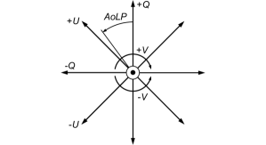
Figure 1: Orientation of the Stokes vector components of Eq. 1, where the beam is propagating out of the paper towards the reader. After the vertical axis ($+Q$) is aligned with a prefered orientation (usually the meridian on-sky), the remaining Stokes vector components are oriented accordingly. The Angle of Linear Polarization ($AoLP$, Eq. 4) is also measured with respect to the $+Q$ direction in counter-clockwise direction.

2.2 The polarimetric imager

Although ideal polarimeters do not exist, such a hypothetical instrument is helpful when we describe the general principles of PDI. Apart from mirrors and lenses the main components of this ideal polarimeter are two (in case of dual-beam) analyzers and detectors (or detector halves). The analyzers can either be two separate polarizers (which require an aditional, preferably non-polarizing beamsplitter upstream) with orthogonal polarization (also called transmission) axes or a polarizing beamsplitter. Let us choose the polarization axis of one analyzer (A1) to be aligned with the $+Q$ direction, and the other analyzer (A2) to be aligned with $-Q$. We can retrieve (or ‘indirectly measure’) the first two components of Eq. 1 by adding and subtracting the measured intensity of both beams ($I_{\mathrm{A1/A2}}$) of light, respectively:

$$I_{\mathrm{}} = I_{\mathrm{A1}}+I_{\mathrm{A2}},$$ (5)

$$Q_{\mathrm{}} = I_{\mathrm{A1}}-I_{\mathrm{A2}}.$$ (6)

We can rephrase Eqs. 5 and 6 to describe the transmission of the analyzers:

$$I_{\mathrm{A1}} = \dfrac{1}{2}(I_{\mathrm{}}+Q_{\mathrm{}}),$$ (7)

$$I_{\mathrm{A2}} = \dfrac{1}{2}(I_{\mathrm{}}-Q_{\mathrm{}}),$$ (8)

where for an ideal polarimeter, $I$ and $Q$ will be equal to their counterparts incident on the telescope ($I_{\mathrm{in}}$ and $Q_{\mathrm{in}}$, respectively).

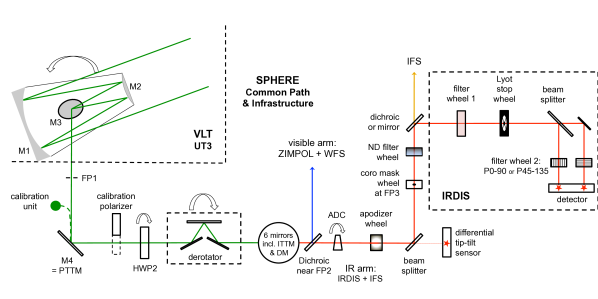
Figure 2: Schematic overview of the telescope and SPHERE/IRDIS, showing the optical components that are relevant for the polarimetric imaging mode. The curved arrows indicate components that rotate during an observation block. Reflections at angles of incidence $\geq 45^{\circ}$ in the instrument are represented with similarly large incidence reflections in the figure. The green beam shows the starlight before color filters are applied, blue represents visible light, red and orange represent NIR light (with the orange beam towards the IFS showing the shorter wavelengths).

To retrieve $U$, we will either need to rotate the analyzers by $45^{\circ}$ or introduce an optical component that can rotate the polarization direction with the same angle. A half-wave ($\lambda/2$) plate (HWP) retards light that is polarized in the direction orthogonal to its fast axis with $\lambda/2$ compared to light that is polarized in alignment with its fast axis. Therefore, a HWP upstream from the beam splitter can be used to rotate the measured polarization angle by $\Delta{AoLP}$ by placing the fast axis of the HWP at an angle of $\Delta{AoLP}/2$ with respect to the polarization axes of the analyzers (Appenzeller 1967). It is possible to retrieve $U$ by placing the HWP at an angle $\theta_{\mathrm{HWP}}=22.5^{\circ}$ with respect to the polarization axis of A1, which changes Eqs. 7 and 8 into: $I_{\mathrm{A1/A2}}=(I\pm U)/2$, and Eq. 6 will yield $U$, instead of $Q$. We now see why the Stokes vector notation is convenient: its components are easilly retrieved from the observables of an ideal polarimeter, which ‘measures’ a Stokes vector unaltered by the telescope and instrument (i.e. $\boldsymbol{S}=\boldsymbol{S}_{\mathrm{in}}$, where $\boldsymbol{S}_{\mathrm{in}}$ is the incident Stokes vector).

Real polarimeters are never ideal: instrumental polarization effects depend on the specific instrument configuration used during observations. For complex instruments, the major instrumental polarization effect is typically the introduction of IP caused by the large number of reflections in the telescope and instrument. We can correct for any IP created downstream of the HWP by recording $Q$ for two HWP angles: $\theta_{\mathrm{HWP}}=0^{\circ}\,\&\,45^{\circ}$ (see e.g. Tinbergen 1996; Witzel et al. 2011; Canovas et al. 2011). The second $\theta_{\mathrm{HWP}}$ changes the signs of the beam’s original $Q$ component but leaves the IP created downstream from the HWP unaltered. Therefore, for non-ideal polarimeters we change the notation of the single-difference computations described by Eq. 6 to measure $Q^{+}=Q+IP$ for $\theta_{\mathrm{HWP}}=0^{\circ}$, and $Q^{-}=-Q+IP$ for $\theta_{\mathrm{HWP}}=45^{\circ}$. Similarly, we rename the single-sum total intensities determined with Eq. 5 for $\theta_{\mathrm{HWP}}=0^{\circ}$ & $45^{\circ}$ as $I_{Q^{+}}$ & $I_{Q^{-}}$, respectively. We then apply the double-difference method to obtain the linear Stokes parameters corrected for IP created downstream of the HWP and the corresponding total-intensity images with the double sum:

$$Q_{\mathrm{}} = \dfrac{1}{2}\left(Q_{\mathrm{}}^{+}-Q_{\mathrm{}}^{-}\right),$$ (9)

$$I_{Q} = \dfrac{1}{2}\left(I_{Q^{+}}+I_{Q^{-}}\right),$$ (10)

$$U_{\mathrm{}} = \dfrac{1}{2}\left(U_{\mathrm{}}^{+}-U_{\mathrm{}}^{-}\right),$$ (11)

$$I_{U} = \dfrac{1}{2}\left(I_{U^{+}}+I_{U^{-}}\right),$$ (12)

where $U^{+}=U+IP$ and $I_{U^{+}}$ are measured with $\theta_{\mathrm{HWP}}=22.5^{\circ}$, while $\theta_{\mathrm{HWP}}=67.5^{\circ}$ yields $U^{-}=-U+IP$ and $I_{U^{-}}$.

The double difference does not remove IP caused by the telescope and instrument mirrors upstream from the HWP, nor does it remove the most important crosstalk contributions. Correcting for these instrumental polarization effects requires that we determine the polarimetric response function for the polarimetric imager, as we do in Sect. 5.2.1 for the polarimetric mode of VLT/SPHERE/IRDIS.

3 Design of the polarimetric mode IRDIS/DPI

In this Section we describe the optical components of VLT/UT3, SPHERE’s Common Path and Infrastructure (CPI) and IRDIS that are most important because they either create instrumental polarization effects, they are useful for calibrations or they can be changed to modify the observational sequence or strategy. These optical components are illustrated in the schematic overview of the telescope and instrument in Fig. 2. Especially reflections at high angles of incidence are highlighted because larger angles are more prone to introduce instrumental polarization effects.

3.1 Telescope and SPHERE common path & infrastructure

SPHERE is installed on the Nasmyth platform of the alt-azimuth Unit Telescope 3. After the axi-symmetric (and therefore non-polarizing) reflections of the primary and secondary mirrors (M1 and M2), the third mirror (M3) of UT3 is used to direct the light towards the Nasmyth focus. M3 introduces the first reflection that breaks axi-symmetry with a $45^{\circ}$ angle of incidence.

Shortly after the beam enters SPHERE we reach Focal Plane 1 (FP1), where a calibration light source can be inserted. The first reflection in the light path within SPHERE is the pupil tip-tilt mirror (PTTM or M4, with a $45^{\circ}$ incidence angle), which is the only mirror in SPHERE that is coated with aluminum. The remaining mirrors of SPHERE are all coated with protected silver for its higher reflectivity. A calibration polarizer with a fixed polarization angle can be inserted in the light path, just before the beam encounters HWP2, the only HWP available for IRDIS/DPI. In field-tracking mode, HWP2 can be rotated for two reasons. The first reason is to switch between four angles (HWP switch angles $\theta_{\mathrm{HWP}}^{s}=0^{\circ},45^{\circ},22.5^{\circ}$ and $67.5^{\circ}$, where the superscript ’s’ is used to distinguish between switch angles and the true angle of HWP2) to measure $Q^{\pm}$ and $U^{\pm}$ with IRDIS. The second reason is to account for field rotation in order to keep the source polarization angle fixed relative to the analyzer for a given HWP2 switch angle in a polarimetric cycle. The next optical component downstream is the image derotator, composed of three mirrors that together form a ‘K’-shape (therefore also called K-mirror, with the subsequent angles of incidence of $55^{\circ}$, $20^{\circ}$ and $55^{\circ}$). The derotator rotates around the optical axis to stabilize either the field or the pupil on the detector. In Appendix A, we have included a detailed description of the tracking laws for HWP2 and the derotator in both field-stabilized and pupil-stabilized mode.

Multiple reflective surfaces with small angles of incidence follow in the AO common path, including the image tip-tilt mirror (ITTM), the $41\,{\times}\,41$ actuator high-order DM and three toric mirrors (Hugot et al. 2012). A dichroic beam splitter separates the light into a visible and a NIR arm just after Focal Plane 2 (FP2). Note that an additional focal plane exists between FP1 and FP2. However, we adopt the nomenclature commonly used in existing literature such as the SPHERE manual. The visible light is reflected by the dichroic beam splitter and sent to SAXO’s wavefront sensor and when required also to ZIMPOL (currently not offered simultaneously with IRDIS or IFS). The NIR beam is transmitted by the dichroic beam splitter, and is then corrected for atmospheric dispersion, determined by the airmass during the observations. Due to the low angles of incidence (${\leq}\,2.17^{\circ}$) on the prisms of the Atmospheric Dispersion Corrector (ADC), it is assumed not to cause significant instrumental polarization effects. The validity of this assumption is left for future investigation. The beam then goes through the apodizer wheel (which allows apodization of the pupil in combination with Lyot coronagraphs) and is sent to a beamsplitter, which transmits $2\%$ of the $H$ band to a differential tip-tilt sensor (DTTS) and reflects the remaining light at $45^{\circ}$ angle of incidence. The (main) reflected beam then encounters the wheel containing NIR coronagraph (focal) masks (Boccaletti et al. 2008; Martinez et al. 2009) in FP3, and the Neutral Density (ND) filter wheel before reaching the final $45^{\circ}$ angle reflection that directs the beam towards IRDIS. For this reflection a dichroic beam splitter is selected when we use IRDIS in concert with IFS. For modes that only use IRDIS, which is currently the case for polarimetry, a mirror is selected instead.

3.2 SPHERE/IRDIS

IRDIS is described in detail by Dohlen et al. (2008). In this subsection and in Fig. 2, we summarize the optical components for a better understanding of the polarimetric performance of the system and for reference later in this paper. The optical components of IRDIS are located within a cryostat cooled to 100 K to reduce thermal background emission. The first optical component inside IRDIS is a common filter wheel (FW1). The filters of FW1 are the only color filters that we can insert for the polarimetic mode, since FW2 contains the analyzer/polarizer pair. Besides narrow-band and spectroscopy filters, FW1 contains four broad-band filters which are offered for DPI (see Table 1).

Table 1: Central wavelength ($\lambda_{c}$), bandwidth ($\Delta\lambda$) and pixel scale for SPHERE/IRDIS broad-band filters available in filter wheel 1. The wavelength and bandwidth are described on the ESO website, the pixel scales come from Maire et al. (2016, 2018). The broad-band filters are listed here as BB_$X$, similar to ESO Observing Blocks (OBs), but they are frequently listed as B_$X$ (on the ESO website and in the headers of FITS files under keyword INS1.FILT.NAME), and as $X$ band in the main text. ^a)The pixel scale for BB_$Y$ has not been calibrated. Therefore, the value for the $Y2$ filter from Maire et al. (2016) has been adopted.

Filter	$\lambda_{c}$ (nm)	$\Delta\lambda$ (nm)	Pixel scale (mas/pix)
BB_$Y$	1043	140	$12.283^{a}\,\pm\,0.009$
BB_$J$	1245	240	$12.263\,\pm\,0.009$
BB_$H$	1625	290	$12.251\,\pm\,0.009$
BB_${K_{s}}$	2182	300	$12.265\,\pm\,0.009$

Next, the beam encounters a Lyot stop wheel that also includes a mask for the pupil obscuration by M2 and its support structure (the ”spider”). Directly downstream from the Lyot stop wheel, the beam is split by the non-polarizing beam splitter plate (NBS). The beam transmitted by the NBS is reflected by an extra mirror in the direction parallel with the beam reflected by the NBS (and therefore with the same angle of incidence as the reflected beam: $45^{\circ}$). The beams are finally reflected by two identical spherical camera mirrors, which focus the beams on the detector (not shown in Fig. 2).

The second filter wheel (FW2) hosting the wire-grid polarizer pairs (P0-90 and P45-135) is located between the camera mirrors and the detector. Finally, the beam reaches the Hawaii-2RG detector, which is mounted on a dither stage and has $2048\,{\times}\,2048$ pixels with 18 $\muup$m pitch. Each of the two orthogonally polarized beams is focused on a separate quadrant ($1024\,{\times}\,1024$ pixels) of the detector, which results in a field of view (FOV) of ${\sim}\,11^{\prime\prime}\,{\times}\,12.5^{\prime\prime}$, and the filter-dependent pixel scales listed in table 1 (Maire et al. 2016, 2018).

3.3 Wire-grid polarizer pairs and beam splitter

The P0-90 analyzer set in FW2 filters the light with polarization angles perpendicular to and aligned with the plane of the Nasmyth platform: the plane in which all reflections downstream from the derotator occur. The P45-135 set polarizes at angles of $45^{\circ}$ and $135^{\circ}$ with respect to this plane. Measurements recorded with P45-135 are highly sensitive to crosstalk introduced by all reflections in this plane. Therefore, we limit the study in Papers I & II to the use of the P0-90 analyzer pair, while using HWP2 to switch between $Q^{\pm}$ and $U^{\pm}$ measurements, which is the default setup for DPI.

The non-polarizing beam splitter is not perfectly non-polarizing, which is corrected for when we use the double difference. Therefore we can use the first-order approximation that it does not introduce new polarization to the beam. Astrophysical objects in the field of high-contrast imaging typically have a very low degree of polarization when integrating the total beam, since this beam is dominated by the central predominantly unpolarized star. The polarizers will only transmit one polarization state each, which means that both beams will loose ${\sim}\,50\%$ of their photons.

4 Polarimetric data reduction

In this Section, we describe the basic steps of the polarimetric data reduction for the IRDIS/DPI mode. In Sect. 5 we will apply this to the data of TW Hydrae as published by van Boekel et al. (2017), and use the results to analyse the polarimetric performance of the system. Because these observations were recorded before we had performed polarimetric calibrations, we encountered unexpected instrumental polarization effects that depend on the specific instrument configuration, and vary during the observing sequence. We will describe and explain these effects in detail based on the polarimetric instrument model of Paper II. In Sect. 6 we compare the reduction of this data after a data-driven correction for instrumental polarization effects with a data reduction after a correction based on the polarimetric instrument model.

To promote general understanding of the underlying principles of the polarimetric data reduction and because our analysis of the data in the subsequent sections required non-standard tests, we did not use the official Data Reduction and Handling (DRH, Pavlov et al. 2008) pipeline but our own custom data reduction routines described below. However, the pre-processing (background subtraction, flat fielding and centering) is very similar to what is done by DRH and therefore described in Appendix B.

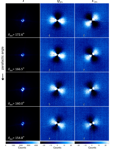
Figure 3: Each row shows the $I$, $Q_{\mathrm{IPS}}$ and $U_{\mathrm{IPS}}$ images (from left to right) for polarimetric cycles with increasing parallactic angle from top to bottom. The on-sky orientation is the same for all panels: north is up, east is left. However, the measured polarization angle (Eq. 4) is changing with derotator angle ($\theta_{\mathrm{der}}$), which we can see with the rotation of the butterfly pattern in clockwise direction. Furthermore, the polarimetric efficiency decreases with $\theta_{\mathrm{der}}$ further removed from $180^{\circ}$, as we can see by the decreasing signal-to-noise ratio in the $Q_{\mathrm{IPS}}$ and $U_{\mathrm{IPS}}$ images.

4.1 Post processing: polarimetric differential imaging

The single-difference images ($Q^{+}$, $Q^{-}$, $U^{+}$, and $U^{-}$) are determined frame by frame for the HWP angles: $\theta_{\mathrm{HWP}}^{s}=0^{\circ}$, $45^{\circ}$, $22.5^{\circ}$, and $67.5^{\circ}$, respectively. The single-difference images obtained from the four frames of each file (per HWP angle) are median combined. $Q$ and $U$ are computed with the double-difference method of Eqs. 9 and 11, for each polarimetric cycle (also called ‘HWP cycles’, containing the four switch angles of HWP2: $\theta_{\mathrm{HWP}}^{s}=0^{\circ}$, $45^{\circ}$, $22.5^{\circ}$, and $67.5^{\circ}$). Accordingly, per HWP angle the corresponding single-sum total-intensity images are created with Eq. 5. With these single-sum images, we create per HWP cycle the double-sum total-intensity $I_{Q}$ and $I_{U}$ images with Eqs. 10 and 12, respectively.

A residual of the read-out columns (see feature c in Fig. 10) remains visible in the double-difference images. Similar to how Avenhaus et al. (2014) removed noise across detector rows from NACO images, we remove these artifacts from the double-difference images by taking the median over the top and bottom 20 pixels (to avoid including signal from the star) on the image per individual pixel column (not the 64 pixel wide read-out column), and subtract this median value from the entire pixel column.

We perform a first-order correction for IP created upstream from HWP2 (i.e. by the telescope and M4) on the $Q$ and $U$ images of each polarimetric cycle. This correction method (as described by Canovas et al. 2011) is based on the assumption that the direct stellar light is unpolarized. We take the median of the $Q/I$ signal over an annulus centered around the star (excluding the coronagraph mask) to obtain the scalar $c_{Q}$ (likewise, we determine $c_{U}$ with $U/I$), multiply this scalar with $I$, and subtract this from the $Q$ image. Hence, the IP-subtracted linear stokes components are:

$$Q_{\mathrm{IPS}} = Q-I_{Q}\cdot c_{Q},$$ (13)

$$U_{\mathrm{IPS}} = U-I_{U}\cdot c_{U}.$$ (14)

The size and location of the annulus over which to measure $c_{Q}$ and $c_{U}$ can be adjusted to suit a particular dataset. Ideally, the annulus should lie in a region that should only contain non-scattered starlight, with high signal in the $I_{Q}$ and $I_{U}$ images. Therefore, the size and location of the annulus depends on the brightness of the central star and the size and shape of the circumstellar material that has been observed.

We now use the possible user-specific derotator offset angle that can be found from the FITS header keyword INS4.DROT2.POSANG, together with the true north correction of $-1.7^{\circ}$ (Maire et al. 2018) to apply a software derotation in order to align all $I_{Q/U}$ and $Q/U_{\mathrm{IPS}}$ with north up and east left on the detector.

4.2 Azimuthal Stokes parameters

To create the final polarization image we have two choices. In the first, most straight-forward method we compute the polarized intensity $PI_{\mathrm{L}}$ according to Eq. 2 for each HWP cycle and median combine these to create a final (less noisy) $PI_{\mathrm{L}}$ image. The problem with this method is that the squares taken in Eq. 2 boost the noise in each image. For example, artifacts seen as a bright positive or negative feature detected at a point in the $Q_{\mathrm{IPS}}$ image where the signal should be ${\sim}\,0$, (on the diagonal ‘null’ lines separating the positive from the negative signal in the $Q_{\mathrm{IPS}}$ images) or a strong positive signal in a region where $Q_{\mathrm{IPS}}$ ought to be negative, will be indistinguishable from true disk signal in the $PI_{\mathrm{L}}$ image. This is actually a general problem we encounter when computing $PI_{\mathrm{L}}$, but even more so when we are dealing with images of short integration times, such as resulting from individual HWP cycles.

In stead, we have used a second option to combine the HWP cycles and create the cleanest image by computing the azimuthal Stokes parameters (Schmid et al. 2006):

$$Q_{\phi} = -Q_{\mathrm{IPS}}\cos{(2\phi)}-U_{\mathrm{IPS}}\sin{(2\phi)},$$ (15)

$$U_{\phi} = +Q_{\mathrm{IPS}}\sin{(2\phi)}\,-U_{\mathrm{IPS}}\cos{(2\phi)},$$ (16)

where $\phi$ describes the azimuth angle, which can be computed for each pixel (or $x,y$ coordinate) as

$$\phi=\arctan{\left(\frac{x_{\mathrm{star}}-x}{y-y_{\mathrm{star}}}\right)}+\phi_{0}.$$ (17)

The $x$ and $y$ positions of the central star in the image are described by $x_{\mathrm{star}}$ and $y_{\mathrm{star}}$, respectively. We can use $\phi_{0}$ to give the azimuth angle an offset if the measured polarization angle is not aligned azimuthally. $\phi_{0}$ is therefore referred to as the polarization angle offset.

Contrary to Eqs. 15 and 16, Schmid et al. (2006) use the notation $Q_{\mathrm{r}}$ and $U_{\mathrm{r}}$, which have flipped signs compared to $Q_{\phi}$ and $U_{\phi}$, respectively. Schmid et al. have chosen their conventions to describe scattered light observations of the planets Uranus and Neptune, which is oriented in radial direction relative to the center of the planet. However, in protoplanery disks, we expect scattered light to produce predominantly azimuthally oriented polarization, which has motivated our choice of signs in Eqs. 15 and 16. Polarization oriented in azimuthal direction (with respect to the position of the star) will be measured as a positive $Q_{\phi}$ signal; radial polarization will show up as a negative $Q_{\phi}$; while polarization angles oriented at $\pm 45^{\circ}$ with respect to azimuthal will result in $\pm U_{\phi}$ signal. Disks that have a high inclination or where multiple scattering is expected to produce a significant part of the scattered light can contain a significant signal in $U_{\phi}$ (Canovas et al. 2015). However, for low-inclination disks we can expect all scattering polarization to be in azimuthal direction. This means that $Q_{\phi}$ will de facto show us $PI_{\mathrm{L}}$, with the benefit that we do not square the noise, resulting in cleaner images. The $U_{\phi}$ image should ideally show no signal at all in this case, which makes it a suitable metric for the quality of our reduction.

5 Instrument-configuration dependence in polarimetric efficiency and polarization angle

5.1 Polarimetric observations of TW Hydrae

We have observed TW Hydrae during the night of March 31, 2015, with IRDIS/DPI. This data was recorded before we became aware of the most severe instrumental polarization effects for SPHERE/IRDIS. Therefore, these data have been recorded without taking recommendations (Sect. 7) into account that optimize the polarimetric efficiency of DPI observations. Furthermore, the near face-on orientation of this disk (inclination $=7^{\circ}$, Qi et al. 2008), allows us to assume azimuthal polarization after scattering, which makes this object an ideal test case to illustrate how instrumental polarization effects alter the incident polarized signal.

The data have been recorded in $H$ band (see Table 1), using field-stabilized mode, while an apodized pupil Lyot coronagraph (Carbillet et al. 2011; Guerri et al. 2011) with a focal plane mask with radius of 93 mas was used. We have performed the observations using a detector integration time (DIT) of 16 s per frame, four frames per file, during 25 polarimetric cycles. This adds up to a total exposure time of 106.7 min.

After creating the double-difference images we removed five HWP cycles with bad seeing and/or AO corrections. Therefore, the final dataset we have used for this analysis contains 20 sets of $Q$, $U$, $I_{Q}$ and $I_{U}$ images.

Figure 3 shows the $I=(I_{Q}+I_{U})/2$, $Q_{\mathrm{IPS}}$ and $U_{\mathrm{IPS}}$ images for four polarimetric cycles observed with increasing parallactic angle for each subsequent panel row. While each $Q_{\mathrm{IPS}}$ and $U_{\mathrm{IPS}}$ panel displays the typical ‘butterfly’ signal of an approximately face-on and axi-symmetric disk, strong variations occur between the polarimetric cycles: the butterflies appear to rotate in clockwise direction and the signal in the $Q_{\mathrm{IPS}}$ and $U_{\mathrm{IPS}}$ images decreases with increasing parallactic angle. Since the observations were taken in field tracking mode, the image of the disk itself does not rotate on the detector, rather the $AoLP$ (Eq. 4) is changing between the polarimetric cycles. We do not expect either the incident (‘true’) Degree or Angle of Linear Polarization to vary with parallactic angle. Notice that $I$ remains roughly constant in Fig. 3, thus a decrease in measured $PI_{\mathrm{L}}$ can only be explained by a decrease in $P_{\mathrm{L}}$. Therefore, the changes in $P_{\mathrm{L}}$ and $AoLP$ must be caused by instrumental polarization effects that depend on the specific telescope and instrument configuration, which varies with the parallactic and altitude angle of the observed star.

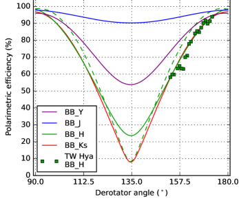
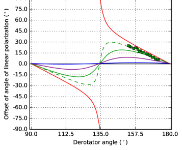
Figure 4: Left: Polarimetric efficiency as a function of derotator angle for all broadband filters listed in Table 1. The green squares show the $H$-band polarimetric efficiencies measured for TW Hydrae scaled to the model curves (Sect. 5.3). The green dashed curve shows the model polarimetric efficiency for the range $0^{\circ}\leq\theta_{\mathrm{der}}\leq 90^{\circ}$ in $H$ band. This filter shows the strongest asymmetry around $\theta_{\mathrm{der}}=90^{\circ}$, which is caused by the non-ideal retardance of HWP2. Right: The model polarization angle offset plotted against $\theta_{\mathrm{der}}$ for the same filters (solid and dashed lines; as before, the dashed line covers the range $0^{\circ}\leq\theta_{\mathrm{der}}\leq 90^{\circ}$). In the ideal case, the polarization angle offset would remain $0^{\circ}$. However, there is a clear dependency on $\theta_{\mathrm{der}}$ for $H$ and $K_{s}$ band, and to a lesser extend for $Y$ band, while the $J$ band remains close to ideal. The polarization angle offsets measured as $\phi_{0}$ for TW Hydrae are plotted as green squares. The deviation of the on-sky data from the model curves is caused by the crosstalk contribution of other optical components.

5.2 Instrumental polarization effects

The calibrations of instrumental polarization effects and the analysis towards a complete Mueller matrix model of the instrument are described in detail in Paper II. In this section we will briefly summarize how we have derived the model from calibration measurements, and describe the instrumental polarization effect of each set of optical components. Here we consider optical components to form a ‘set’ when they share a fixed reference frame, i.e. a common rotation of the set of components. For the last set of components (CPI + IRDIS components downstream of the derotator) we only fit the diattenuation, since crosstalk is absent because all reflections are aligned with the anlyzers.

In Sect. 5.3 we use this polarimetric instrument model to explain variations detected in the degree and angle of linear polarization in the data of TW Hydrae. Based on the polarimetric instrument model we have devised a correction method in Paper II. In Sect. 6 of this paper we apply this correction method to retrieve the true incident polarization for the observations of TW Hydrae.

5.2.1 From calibrations to polarimetric instrument model

In Paper II, we have used the internal light source with a calibration polarizer to create $100\%$ polarized light, and measured the linear Stokes parameters for a wide range of instrumental configurations. We then defined the measured degree of linear polarization for the $100\%$ polarized incident light to be equal to the polarimetric efficiency for this configuration. For each set of optical components including and downstream of the HWP, we have fitted the measured Stokes parameters to the wavelength-dependent retardance of this set of components. Similarly, we have calibrated the diattenuation of these sets of optical components with the internal light source, this time without the inclusion of a calibration polarizer to insert nearly unpolarized incident light.

We have calibrated the diattenuation of the telescope and M4 (both located upstream from the HWP) by observing unpolarized stars at various altitude angles of the telescope. The retardances of these optical components have been determined analytically using the Fresnel equations and literature values for the complex refractive index of the coating material. With the diattenuation and retardance we have computed the wavelength-dependent $4\,{\times}\,4$ Mueller matrices for each set of optical components that share a reference frame. The combination of the Mueller matrices for all optical components forms our polarimetric instrument model.

5.2.2 The derotator and HWP2

The left-hand panel of Figure 4 shows the polarimetric efficiency curves against derotator angle ($\theta_{\mathrm{der}}$) for the four broadband filters of IRDIS. The solid lines show the polarimetric efficiency derived from the Mueller matrix model for the optical system for $90^{\circ}\leq\theta_{\mathrm{der}}\leq 180^{\circ}$, while the green dashed line shows this for $0^{\circ}\leq\theta_{\mathrm{der}}\leq 90^{\circ}$ in $H$-band only. These green solid and dashed curves clearly do not overlap, and the same is true for the other filters (not shown). This asymmetry across $\theta_{\mathrm{der}}=90^{\circ}$ in the polarimetric efficiency curve is caused by a non-ideal behavior of HWP2, i.e. the retardance $\neq\lambda/2$ (see Paper II). A dramatic decrease in polarimetric efficiency is seen for $\theta_{\mathrm{der}}\,{\approx}\,45^{\circ}$ and $135^{\circ}$ in the $H$ and $K_{s}$-band filters, while $Y$-band and especially the $J$-band filters show a much better polarimetric efficiency curve.

The right-hand panel of Figure 4 shows how the polarization angle offsets oscillate around $0^{\circ}$ (which would be the value in the ideal case of no crosstalk) for the model (solid and dashed lines) and the data (green squares). While this oscillation is only marginally visible for $J$ band, with a maximum deviation from ideal $<4^{\circ}$; it is $<11^{\circ}$ in $Y$, and can reach up to $34^{\circ}$ in $H$. For $K_{s}$ band, the polarization angle offset does not even return to its equilibrium and continues rotating beyond $\pm 90^{\circ}$ (where a rotation of $+90^{\circ}$ is indistinguishable from $-90^{\circ}$).

The strong dependence of the polarization angle offset and polarimetric efficiency on $\theta_{\mathrm{der}}$ in $H$ and $K_{s}$ band are predominantly caused by crosstalk induced by the retardance of the derotator, which is close to that of a quarter-wave ($\lambda/4$) plate at these wavelengths. With these retardances, the derotator causes a strong linear to circular polarization crosstalk. This crosstalk means that when we use the wrong observing strategy we can lose up to $95\%$ of incident linearly polarized signal, which is ultimately the information carier we aim to measure. Because other optical components (e.g., HWP2) contribute to this loss of polarization signal as well, we list the polarimetric efficiencies for the least favorable instrumental configuration in Table 2.

Table 2: Lowest polarimetric efficiencies reached at the least favorable instrumental set-up. The values are determined with the polarimetric instrument model (Paper II) for the broad-band filters described in Table 1.

$Y$ ($\%$)	$J$ ($\%$)	$H$ ($\%$)	${K_{s}}$ ($\%$)
54	89	5	7

5.2.3 The telescope and SPHERE’s first mirror

Table 3: IP (in percent of the total intensity) induced by the telescope mirrors and M4 before and after recoating of the M1 and M3. The values are shown at optimal, nearly crossed configuration of the reflection planes of M3 and M4 (at $a=87^{\circ}$, with $a$ the altitude angle of the Unit Telescope), and worst, close to aligned reflection planes ($a=30^{\circ}$: the lowest altitude at which the ADC can correct for atmospheric dispersion) for the IRDIS’ broadband filters.

Date	$a$ (∘)	$Y$ ($\%$)	$J$ ($\%$)	$H$ ($\%$)	${K_{s}}$ ($\%$)
Before	87	0.58	0.42	0.33	0.29
16-04-2017	30	3.5	2.5	1.9	1.5
After	87	0.18	0.12	0.07	0.06
16-04-2017	30	3.0	2.1	1.5	1.3

On April 16, 2017, UT3’s M1 and M3 have been recoated, resulting in a more effective cancellation of IP when M3 and M4 are in crossed configuration (when looking at or close to zenith). Therefore, we present the lowest and highest IP values for each broadband filter as measured before and after recoating in Table 3.

5.3 Explaining TW Hydrae data with the instrument model

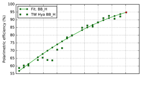
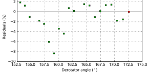
Figure 5: Top: Polarimetric efficiency modeled (solid line) for the same derotator and HWP2 angles as used during the observation of TW Hydrae (squares). Note that the polarimetric efficiencies measured for the HWP cycles of TW Hydrae are only determined relative to the other HWP cycles. We therefore scaled all data points such that the first cycle (red square, with the highest polarimetric efficiency) matches the value of the model. Bottom: Residuals between the model and the polarimetric efficiencies obtained for TW Hydrae.

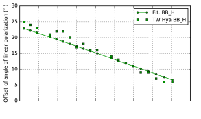
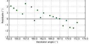
Figure 6: Top: Expected polarization angle offsets of the same model (solid line) as used in Fig. 5; and the polarization angle offset angles ($\phi_{0}$ of Eq. 17) of TW Hydrae (squares) with respect to azimuthal polarization. Bottom: Residuals between the model polarization angle offsets and $\phi_{0}$ retrieved for TW Hydrae.

During the observation of the 20 HWP cycles, the derotator has rotated from $\theta_{\mathrm{der}}$$\,=173.2^{\circ}$ to $\theta_{\mathrm{der}}$$\,=152.6^{\circ}$ ($\Delta$$\theta_{\mathrm{der}}$$\,=-20.6^{\circ}$). To account for the variation of the measured $AoLP$ between the HWP cycles, we have determined the correct value for the polarization angle offset $\phi_{0}$ for each cycle separately, based on the assumption that the polarization is oriented in azimuthal direction, and therefore $U_{\phi}$ should be 0. We have achieved this by computing the sum over the absolute signals measured for the pixels in a centered annulus in the $U_{\phi}$ image for a range of $\phi_{0}$ values: $c_{U_{\phi}}(\phi_{0})$. We have selected the $\phi_{0}$ value which yielded the lowest $c_{U_{\phi}}(\phi_{0})$. We have derived the relative polarimetric efficiency by measuring the absolute signal over an annulus in the $Q_{\phi}$ image for each cycle, and dividing these values by that of the highest (coincidentally the first) HWP cycle. During the observing sequence of TW Hydrae the polarimetric efficiency has decreased with ${\sim}\,40\%$.

The green squares in Fig. 4 represent the relative polarimetric efficiency (left panel) and the polarization angle offset (right panel) for the TW Hydrae measurements. For this dataset we know neither the incident nor measured $P_{\mathrm{L}}$ (instead, we measure $Q_{\phi}\approx PI_{\mathrm{L}}$ and do not know $I$ of the disk) to determine the absolute value of the polarimetric efficiency. However, during the observations, $Q_{\phi}$ is expected to be linearly proportional to the polarimetric efficiency. Therefore, we have measured for each HWP cycle the mean $Q_{\phi}$ in a fixed annulus around the star and scale the images such that the highest mean value (from the first HWP cycle) matches the model’s polarimetric efficiency in $H$.

Although the polarimetric efficiency is rather well explained with the $H$-band model curve (green solid line), the polarization angle offset deviates from the model. The models shown in Fig. 4 are created for the simplest configuration, where all instrument settings have been kept constant except $\theta_{\mathrm{der}}$, while during the on-sky observations many optical components have changed position due to their field-tracking laws, such as HWP2 and the telescope altitude angle.

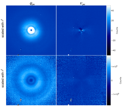
Figure 7: Final $Q_{\phi}$ (left) and $U_{\phi}$ (right) images of TW Hydrae. Both $Q_{\phi}$ and $U_{\phi}$ are displayed with identical linear scale, and either unscaled (top) or scaled with $r^{2}$ (bottom) to compensate for the decrease of stellar flux with distance. All four panels are shown with North up and East to the left for the same field of view of $4.9^{\prime\prime}\,{\times}\,4.9^{\prime\prime}$ or up to a separation of $r=2.45^{\prime\prime}$ from the star in both RA ($-x$-axis) and Dec ($+y$-axis).

To account for these additional changes in configuration, we use the instrument model to compute the polarimetric efficiency and polarization angle offset for the same instrument configuration as was used during the observations of TW Hydrae. We compare the predicted polarimetric efficiencies and polarization angle offsets with on-sky observation polarimetric efficiencies in Fig. 5 and polarization angle offsets in Fig. 6.

The model predictions are very succesful at explaining the changes in polarimetric efficiency and polarization angle. We see some clear outliers in both Figs. 5 and 6 at $\theta_{\mathrm{der}}\approx 139^{\circ}$, which are most likely caused by a poor fit of $\phi_{0}$ for these HWP cycles. This shows that our comparison is limited by the accuracy of the polarimetric efficiency measurement in the data rather than that of the model.

6 Comparison between data reduction with $U_{\phi}$ minimization and model-based correction

After Sect. 5.1 we paused our post-processing of the data to analyze the instrumental polarization effects that cause the detected variations in $P_{\mathrm{L}}$ and $AoLP$ for TW Hydrae in Sect. 5.2 and 5.3. We have succesfully implemented these lessons to create a detailed polarimetric instrument model and a model-based correction method for the instrumental polarization effects (see Paper II). In this section we will compare post-processing based on this correction method with the best post-processing we have performed without using the correction method, where we have corrected for residual $IP$ empirically by minimizing signal in $U_{\phi}$. We will continue with the empiric correction method from where we stopped in Sect. 5.1.

6.1 Refining the reduction by minimizing $U_{\phi}$

We determine $\phi_{0}$ as described in Sect. 5.3. Then we improve our centering by shifting the $Q_{\mathrm{IPS}}$ and $U_{\mathrm{IPS}}$ images with a range of $x$ and $y$ steps to find the minimum $c_{U_{\phi}}(x,y)$ value. Because the improved centering will affect the minimization process with which we found $\phi_{0}$, we repeat the minimization of $c_{U_{\phi}}(\phi_{0})$ on the centered data, and find $\phi_{0}$ with increasing values between $6^{\circ}\leq\phi_{0}\leq 25^{\circ}$ for the 20 HWP cycles. A final $U_{\phi}$ minimization is performed to enhance our IP correction: we find the minimum of $c_{U_{\phi}}$ by searching a grid of constants $c^{i}_{Q}$ and $c^{j}_{U}$ with which we replace $c_{Q}$ and $c_{U}$ in Eqs. 13 & 14 to compute $Q_{\mathrm{IPS}}$ and $U_{\mathrm{IPS}}$, respectively. For each point ($i,j$) in the grid, we compute $U_{\phi}$ with Eq. 16 and addopt the $c^{i}_{Q}$ and $c^{j}_{U}$ values that yield the smallest value of $c_{U_{\phi}}$.

The $U_{\phi}$ minimizations are performed and $Q_{\phi}$ & $U_{\phi}$ are computed per HWP cycle. At this stage we determine the polarimetric efficiency as described in Sect. 5.3. The final $Q_{\phi}$ & $U_{\phi}$ images shown in Fig. 7 are created by median combining the 20 $Q_{\phi}$ and $U_{\phi}$ images determined per cycle, respectively.

6.2 Correcting observations with the instrument model

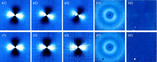
Figure 8: a1, a2, & a3) $Q_{\mathrm{IPS}}$ images of three HWP cycles with $\theta_{\mathrm{der}}=169.7^{\circ},162.0^{\circ}$, and $154.1^{\circ}$, respectively. These images are created with the $U_{\phi}$ minimization method (Sect. 6.1). We can clearly see the buttefly patterns rotate in clockwise direction and the signal decrease from left to right. b) When we use the assumption of azimuthal polarization, we can find the correct $\phi_{0}$ for each HWP cycle and compute the final $r^{2}$-scaled $Q_{\phi}$ (b1) and $U_{\phi}$ (b2) images (Sect. 6.1). Because we have used the assumption that we know the Angle of Linear Polarization at each point, we cannot claim to have determined the $AoLP$ in this image. c) When we apply the correction method to the $Q$ and $U$ images, we retrieve the best approximation of the incident $Q$ and $U$ images (Sect. 6.2). The displayed $Q$ images (for the same $\theta_{\mathrm{der}}$ as panel a) contain the ideal orientation of the butterflies and are corrected for the reduced polarimetric efficiency. However, the latter does not improve the signal to noise (illustrated by the increased noise in panel c3). d1 & d2) The IRDAP-corrected $Q_{\phi}$ and $U_{\phi}$ image. Because we no longer need the assumption that we know the $AoLP$ a priori, we can use $Q$ and $U$ after the correction method to determine the $AoLP$ in our final reduction.

In Sect. 5.3 we show that the polarimetric instrument model can very well explain the variations in $P_{\mathrm{L}}$ and $AoLP$ measured in the data as instrumental polarization effects. In Paper II, we have presented a highly-automated data-reduction pipeline (IRDAP) that contains a correction method based on this instrument model. We have reduced the TW Hydrae data with IRDAP, without any prior correction for instrumental polarization effects (i.e. we did not apply Eqs. 13 and 14 or $U_{\phi}$ minimization). For illustrative purposes, we have also applied the model correction to three individual polarimetric cycles with $\theta_{\mathrm{der}}=169.7^{\circ},162.0^{\circ}$, and $154.1^{\circ}$ of this dataset. Fig. 8 shows the images as reduced with the method described in Sect. 6.1 and the result of the IRDAP corrections. The $Q_{\mathrm{IPS}}$ images of these three HWP cycles reduced with $U_{\phi}$ minimization are shown in panels a1, a2 and a3, the final $Q_{\phi}$ and $U_{\phi}$ images of this reduction method are shown in panels b1 and b2, respectively. The $Q$ images for the same HWP cycles of panel a are shown after application of the correction method in panels c1, c2 and c3, and the final IRDAP-reduced $Q_{\phi}$ and $U_{\phi}$ images are shown in panels d1 and d2, respectively.

6.3 Comparison of reduction methods

While the $Q_{\mathrm{IPS}}$ images of Fig. 8a show the rotation of the butterfly ($\phi_{0}\neq 0$) caused by crosstalk, the corrected $Q$ images of panel c are clearly oriented such that $\phi_{0}\approx\,0^{\circ}$. Although the IRDAP-corrected $Q$ images display a surface brightness which is approximately the same for all three images in panel c, the loss of polarization signal in the three $Q_{\mathrm{IPS}}$ images (from a1 to a3) is still visible as a decrease of the signal-to-noise ratio when comparing panel c3 with c1.

The azimuthal direction of the true polarization angle was used as an assumption in our reduction of $Q_{\phi}$ in Sect. 6.1. Therefore, we cannot claim to have derived the angle of linear polarization in panel b1. However, since we do not need to assume a-priori knowledge about $AoLP$ to compute the final $Q_{\phi}$ image of panel d1, we can confidently claim to have determined the $AoLP$. As a result, the $U_{\phi}$ image of panel d2, created with $\phi_{0}=\,0^{\circ}$ is even cleaner (especially at small separations) than the $U_{\phi}$ image of panel b2.

Although the $Q_{\phi}$ images produced with both methods (Fig. 8 b1 & d1) show to a large degree the same disk structures, the correction method will always produce more accurate polarization measurements than reduction methods without a model-based correction. When the aim of the observation is to perform a qualitative analysis of the data, such as describing the large-scale morphology of disks, a more conventional reduction method may suffice for a face-on disk such as TW Hydrae. However, the loss of polarization signal as displayed between panels a1, a2 & a3 illustrates that our combination of data from multiple polarimetric cycles will result in very poorly constrained polarimetric intensity measurements. More importantly, when we observe disks at larger inclination, especially in $H$ or $K_{s}$ band, even qualitative analysis of the data is likely to become skewed when the instrumental polarization effects are not corrected properly. In Paper II we illustrate that the shape of $Q_{\phi}$ and especially $U_{\phi}$ images of the disk around T Cha look much more reliable (i.e. more similar to radiative-transfer model predictions, Pohl et al. 2017)) after applying the correction method.

7 Recommendations for IRDIS/DPI

7.1 Observing strategy to optimize polarimetric performance

Previous publications (e.g., Garufi et al. 2017) have demonstrated that the polarimetric mode of IRDIS is a very effective tool to image the scattering surface of protoplanetary and debris disks. However, the analysis of the TW Hydrae data presented in this paper illustrate that the polarimetric efficiency can be negatively affected when the instrument configuration is not optimized. When using IRDIS/DPI in field-tracking mode, we recommend the following adjustments to the observing strategy to avoid a loss of polarized signal:

• When no strict wavelength requirements are present and the disk surface brightness is expected to be gray in the NIR: use $J$ band to achieve a ${>}\,90\%$ polarimetric efficiency, which is nearly independent of the remaining instrumental setup.

• However, most young stars are red, causing their disks to scatter more light in $H$ than in $J$ band. If the previous recommendation to use $J$ band cannot be met and the $Y$-, $H$-, or $K_{s}$-band filters are used, avoid the use of derotator angles $22.5\lesssim|\theta_{\mathrm{der}}|\lesssim 67.5^{\circ}+n\cdot\,90^{\circ}$, with $n\in\mathbb{Z}$.

The latter recommendation ensures a polarimetric efficiency $\geq 70\%$. This constraint on $\theta_{\mathrm{der}}$ can be achieved with two simple steps:

1. Within ESO’s Phase 2 Proposal Preparation tool (P2PP or P2), split the total observation within an observing block (OB) into parts (templates) where the difference between $p$ and $a$ does not vary by more than $90^{\circ}$, resulting in $|\Delta\theta_{\mathrm{der}}|<45^{\circ}$, because $\theta_{\mathrm{der}}\propto(a-p)/2$;

2. For each template, the $\theta_{\mathrm{der}}$ constraint can be determined by finding the average parallactic and altitude angles and applying a derotator (position angle) offset of:

   $$\mathrm{INS.CPRT.POSANG}=\,{<}\,p-a\,{>}+\,n\,\cdot\,180^{\circ},$$ (18)

   with $n\in\mathbb{Z}$, and $<>$ indicating the average values.

The parallactic and altitude angle can be determined by:

$$p = \arctan\left(\frac{\sin{({HA})}}{\tan{{(\phi)}}\cos{(\delta)}-\sin{(\delta)}\cos({HA})}\right),$$ (19)

$$a = \arcsin\left(\sin{(\delta)}\sin{(\phi)}+\cos{(\delta)}\cos{(\phi)}\cos{(HA)}\right),$$ (20)

where $\phi=-24.6^{\circ}$ is the latitude of the VLT at the Paranal observatory, $\delta$ is the declination of the star, and ${HA}$ is the Hour Angle of the star = Local Sidereal Time (LST) - Right Ascension (RA).

The required derotator offset will be strongly dependent on the exact start of the observation template. During visitor mode observations, where the observer is present at the observatory, the optimal derotator offset can be included in the OBs just before the start of the observations. During remote service mode observations, the observer does not know at what time the observation will start and therefore not what the optimal value will be for INS.CPRT.POSANG. This problem can be solved by either including a list of LST values and the corresponding derotator position angle offsets to the README file of the OB, or by providing LST constraints and a corresponding optimal derotator offset to the OB, preferably around a time when the parallactic angle does not change too much during the observation.

When the optimal value for INS.CPRT.POSANG is used, the mean $\theta_{\mathrm{der}}$ lies at either $0^{\circ}$ or $90^{\circ}$, which orients the derotator horizontal or vertical with respect to the Nasmyth platform. This orientation will cause little or no crosstalk and therefore limited loss of polarized signal and a close to ideal polarization angle.

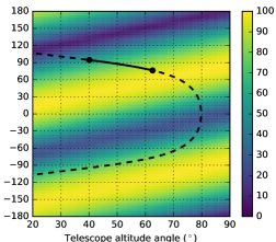
Figure 9: The polarimetric efficiency in $H$ band as a function of the parallactic angle and altitude angle, when the derotator is in field-tracking mode without an additional derotator offset. The dashed line shows the parallactic and altitude angle of TW Hydrae across the sky, with the solid line showing the angles during the SPHERE observation. We clearly see that using default derotator settings (North up on the detector) will give us mediocre polarimetric efficiencies.

Figure 9 shows the polarimetric efficiency mapped for $p$ and $a$ without the application of a derotator offset. Given the path traveled by TW Hydrae during our observations shown with the black solid line (${<}\,p\,{>}\approx 90^{\circ},{<}\,a\,{>}\approx 50^{\circ}$), we could have avoided the loss of polarization signal by providing a derotator position angle offset of $\mathrm{INS.CPRT.POSANG}=90-50=40^{\circ}$, rotating the derotator by $20^{\circ}$. We did not apply this derotator offset because we were not aware of the strong crosstalk for IRDIS/DPI at the time of these observations.

7.2 SPHERE design upgrades

7.2.1 HWPs 1 & 3 to reduce instrumental polarization effects

The most thorough way to reduce instrumental polarization effects for IRDIS would be to introduce two more HWPs in the optical path. A HWP1 at the same location as for ZIMPOL, in between M3 and M4, can keep the IP induced by both mirrors perpendicular to let them cancel out. We then use HWP2 in a slightly different fashion: rather than aligning the to-be-measured polarization angles with the analyzers, it aligns the desired polarization with the reflection plane of the derotator, as it does for ZIMPOL (Schmid et al. 2018). Similar to ZIMPOL, this new rotation law for HWP2 requires that we install a third HWP to align the desired polarization angle with the transmision axes of IRDIS’ polarizers. We recommend to install this HWP3 directly downstream of the derotator, to completely remove all crosstalk.

We are aware that the diverging beam downstream of the derotator is relatively large, which might make it difficult to produce a HWP that is large enough. The feasibility of this recommendation is yet to be determined. Alternatively, as for ZIMPOL, HWP3 could be installed further down the optical path when the beam starts to become smaller (e.g., between the apodizer wheel and the DTTS beam splitter, before large incidence-angle reflections are encountered by the beam).

7.2.2 Recoating of the derotator to reduce retardance

As we describe in Sect. 5.2.2, due to its unfavorable retardance (nearly $\lambda/4$ in $H$ and $K_{s}$) the derotator is by far the largest contributor of crosstalk and hence loss of polarimetric efficiency. Therefore, an alternative recommendation to reduce the loss of polarimetric efficiency for IRDIS is to recoat the three mirrors of the derotator with a coating that yields a total retardance of the derotator close to $\lambda/2$ in all filters. We are currently investigating the feasibility to apply a coating to the derotator that yields ${\sim}\,\lambda/2$ retardance over the very broad wavelength range required by ZIMPOL and IRDIS combined. Whether HWP3 is still desired after recoating depends on how close the retardance of the new coating is to the ideal value for the full wavelength range covered by IRDIS.

7.2.3 A polarizing beam splitter to increase throughput

The throughput of the combination of non-polarizing beam splitter plate + wire-grid polarizers is ${\sim}\,50\%$, as discussed in Sect. 3.3. Replacing the non-polarizing plate with a polarizing beam splitter plate will immediately increase the throughput with a factor ${\sim}\,2$. An additional result of this upgrade will also be that polarimetry is offered ’for free’ for any observation performed with IRDIS. Polarimetry-for-free will allow a substantial boost of the science output of the instrument by serendipitous discoveries of polarized circumstellar disks during planet-hunting surveys. The observer can choose whether to use full HWP cycles if polarimetry is not the primary objective. However, one should always consider at least cycling two HWP angles set $45^{\circ}$ apart (e.g., $Q^{\pm}$), especially for DBI to avoid confusing polarized signal for a spectral feature. This necessity of the HWP requires that we need to investigate whether inlcuding this optical component affects the contrast of DBI, classical imaging, but also IFS observations.

7.2.4 IRDIS polarimetry & IFS observations simultaneously

An important first test for the desirability of IRDIS polarimetry-by-default is to do combined IRDIS/DPI + IFS observations. Although this combination is currently not offered, it does not require any changes in design, only software (new observing templates). The instrumental polarization effects of inserting a dichroic beam splitter in stead of a mirror (to fold the beam towards IRDIS) is expected to be negligible, because it would cancel after the double difference. The largest unknown will be the effect of the HWP for IFS observations. This test is valuable, not only to investigate if a polarizing beam splitter should be installed in IRDIS. If the outcome is indeed that IRDIS/DPI observations do not affect the IFS and vice-versa, we again open a new window for increased science output per observation that can be used almost immediately. This new mode would be very helpful for substellar companion searches close to stars that are surrounded by disks, or disk-searches while characterizing substellar companions.

8 IRDIS/DPI compared to contemporary AO-assisted imaging polarimeters

In this Section we make a brief comparison between the polarimetric mode of SPHERE/IRDIS and the major contemporary AO-assisted high-contrast polarimetric imagers operating in the near infrared: GPI and NACO. The designs of both GPI and SPHERE are primarily focused on the minimization of wavefront errors (Macintosh et al. 2014; Beuzit et al. 2019), which is crucial for the detection of planets at high contrasts and small separation from the central star. Polarimetry had a much lower priority in the design choices, which resulted in designs that are suboptimal for the polarimetric performance of both instruments.

However, the extreme AO systems of both GPI (Poyneer et al. 2014) and SPHERE (Fusco et al. 2006) turn out to be crucial for their polarimetric imaging modes. Although a detailed comparison between the perfomance of these AO systems and the older generation Nasmyth Adaptive Optics System (NAOS, Rousset et al. 2003) of NACO lies outside the scope of this study, the reported performances of these systems allow for some obvious conclusions. The AO systems of SPHERE and GPI can both run at ${\sim}1$ kHz and control a high-order DM containing $41\,{\times}\,41$ and $64\,{\times}\,64$ actuators, respectively, while NAOS can control its DM with 185 active actuators at either $444$ Hz or $178$ Hz for its visible light or NIR wavefront sensor, respectively. The resulting point spread functions reach high Strehl ratios (${\gtrsim}\,90\%$ in $H$-band) and remain very stable for extended periods of time for both SPHERE and GPI, while NACO reaches typical Strehl ratios of ${\gtrsim}\,50\%$ in $K_{s}$ band and ${\gtrsim}\,30\%$ in $H$ band. Another important characteristic of the three AO systems is the limiting magnitude at which these systems can still operate. These magnitude limits are $I\approx 10$ mag for GPI (Macintosh et al. 2014), $R\approx 15$ mag for SPHERE (Beuzit et al. 2019), and $V\approx 16$ mag and $K\approx 14$ mag for NACO (Rousset et al. 2003). These limits make SPHERE and NACO particularly well-suited to perform polarimetric imaging observations of relatively faint objects, such as most nearby T Tauri stars.

There are many differences in the designs of the polarimetric modes of NACO, GPI and SPHERE/IRDIS. SPHERE is mounted on the Nasmyth platform of the telescope and employs an internal image derotator to stabilize the field or pupil. NACO is also mounted at the Nasmyth focus, but contrary to SPHERE it is attached to the derotator flange of the telescope support structure (Lenzen et al. 2003). This Nasmyth derotator rotates the complete instrument to track either field or pupil, although pupil tracking is rarely used for the polarimetric imaging mode of NACO. GPI is mounted at the telescope Cassegrain focus, which avoids the need of a tertiary telescope mirror. It has no image derotator, which allows only pupil stabilized imaging, not field tracking.

The three instruments contain many internal reflections before the light beam reaches the detector. Because the double difference removes the $IP$ produced by the optical components downstream of the HWP, the location of the HWP is important for the polarimetric performance of the instruments. While HWP2 of SPHERE/IRDIS is situated early in the optical train, directly after the first internal reflection within the instrument (between M4 and the derotator, see Fig. 2), GPI and NACO have their HWPs installed after many reflective surfaces (Perrin et al. 2010; Witzel et al. 2011, respectively).

As a result of these design choices, the $IP$ of SPHERE originates only from the telescope and M4, and therefore varies with telescope altitude angle (see Table 3). The $IP$ of NACO is produced by the telescope and the reflections in the NAOS AO system. Because NACO rotates with respect to the telescope in field-tracking mode, its $IP$ also depends on the telescope altitude angle. Millar-Blanchaer et al. (in prep.) measure the $IP$ of NACO in pupil tracking (most favorable instrument configuration) in $H$ band, and determine the $IP$ to be comparable to that of SPHERE/IRDIS at low altitude angles (worst configuration). The $IP$ of GPI originates primarily from the reflections in the instrument upstream from the HWP. Millar-Blanchaer et al. (2016) measure average $IP$ values that are very comparable to SPHERE/IRDIS.

The crosstalk of SPHERE/IRDIS is predominantly caused by the derotator and HWP2, which can result in a large decrease in polarimetric efficiency (Sect. 5.2.2). Since GPI does not have an image derotator and has all reflections aligned in a single plane, the retardance of the instrument is very small (Millar-Blanchaer et al. 2014) compared to SPHERE/IRDIS. In NACO, the crosstalk is predominantly caused by M3 and the optical components of NAOS. Because the HWP is located downstream of these components, the resulting polarimetric efficiency differs between measurements of Stokes $Q$ and $U$, when $Q$ is aligned with the optical axes of the polarizing beam splitter. Avenhaus et al. (2014) determine the polarimetric efficiency of Stokes $U$ to be ${\sim}\,60\%$ relative to Stokes $Q$ for NACO. Although a similar effect may be expected for GPI due to the location of the HWP, to the best of our knowledge no differences in polarimetric efficiency between $Q$ and $U$ have been reported in literature.

Both Millar-Blanchaer et al. (2016) and Van Holstein et al. (2017) show for GPI and SPHERE/IRDIS, respectively, that the polarized contrast at separations ${\gtrsim}\,0.3"$ is dominated by the photon and readout noise and therefore scales with the square root of the exposure time. Both papers report very similar polarized contrasts of $10^{-6}-10^{-7}$ at a separation of 0.4”, while de Juan Ovelar (in prep.) has measured a polarized contrast of ${\sim}\,10^{-6}$ at a separation of 1” for NACO. We can therefore conclude that the polarimetric performances of GPI and SPHERE/IRDIS are very similar for relatively bright stars ($R\approx 6$ mag). Due to their extreme AO systems and small differential wavefront errors, SPHERE/IRDIS and GPI reach much higher polarized contrasts than NACO at sub-arcsecond separations from the star.

9 Conclusions

The polarimetric mode of SPHERE/IRDIS has been very succesful at imaging protoplanetary disks at resolutions and polarized contrasts close to the star that were not attainable with the previous generation of polarimetric imagers. Because the design was mainly driven by non-polarimetric requirements, its performance is strongly dependent on the observing strategy, as we have illustrated with the observations of TW Hydrae. When the observing strategy is not optimized, polarimetric crosstalk can cause the efficiency to drop towards ${\sim}\,5\%$ in $H$ and $K_{s}$ band; polarimetric efficiency remains above $54\%$ in $Y$ band and above $89\%$ in $J$ band. Low polarimetric efficiency means that we lose polarization signal, which is what we aim to detect in DPI mode. Crosstalk also causes a polarization angle offset up to ${\sim}\,30^{\circ}$ in $H$- and more in $K_{s}$. We have demonstrated that the polarimetric instrument model described in Paper II can be used to explain and correct for the variations in polarimetric efficiency and polarization angle offset due to crosstalk observed in the TW Hydrae data.

The work presented in Papers I & II show that instrumental polarization effects are significant but also that this a-posteriori work allows a very high quality data product, which is above expectations given the loose constraints on the design requirements. Optimal results can be obtained from IRDIS/DPI observations when two important considerations are taken into account: 1) Adjust the observating strategy beforehand as described in Sect. 7.1 to minimize a decrease in polarimetric efficiency. 2) Apply the correction method described in Paper II, and included in the IRDAP pipeline, to correct the data for instrumental polarization effects.

Appendix A Tracking laws for HWP2 and the derotator

A.1 Field tracking

A.1.1 The derotator

Field tracking is the default setting for the polarimetric imaging mode of IRDIS. In this setting, the derotator control law keeps the image with north up on the detector, (except for the true-north offset described in Sect. 4.1) which is given by:

$$\theta_{\mathrm{der}}=\frac{1}{2}\left(-p+a\right)+\frac{1}{2}\eta,$$ (21)

with $\theta_{\mathrm{der}}$ the derotator angle, $p$ the astronomical object’s parallactic angle (FITS header keyword: TEL.PARANG.START), and $a$ the altitude angle of the Unit Telescope (TEL.ALT). The user-defined position angle offset $\eta$ of the image (INS4.DROT2.POSANG) can be altered by changing the value of INS.CPRT.POSANG in the Observing Block (OB), as described in Sect. 7. The header value of the derotator angle is computed as:

$$\mathrm{INS4.DROT2.BEGIN}=\theta_{\mathrm{der}}+n\cdot 360^{\circ},$$ (22)

with $n\in\mathbb{Z}$.

A.1.2 The half-wave plate

The HWP2 control law for field-tracking with IRDIS/DPI (implemented in March, 2015) keeps the polarization direction aligned with the analyzers, and is given by:

$$\theta_{\mathrm{HWP}} = -p+a+\frac{1}{2}\left(\eta+\gamma\right)+\theta_{\mathrm{HWP}}^{s}$$ (23)

$$= 2\theta_{\mathrm{der}}+\frac{1}{2}\left(\gamma-\eta\right)+\theta_{\mathrm{HWP}}^{s},$$ (24)

with $\theta_{\mathrm{HWP}}$ the HWP angle, and $\gamma$ a position angle offset of the linear polarization direction due to a user-defined HWP2 offset (INS4.DROT3.GAMMA, to be changed by adjusting SEQ.POL.OFFSET.GAMMA in the OB). $\theta_{\mathrm{HWP}}^{s}$ is the switch angle used during HWP cycles as described in Sect. 3.1. When SEQ.IRDIS.POL.STOKES is set to ”QU” in the OB, $\theta_{\mathrm{HWP}}^{s}$ cycles through the angles $0^{\circ},45^{\circ},22.5^{\circ}$ and $67.5^{\circ}$, but only through $0^{\circ}$ an $45^{\circ}$ if SEQ.IRDIS.POL.STOKES is set to ”Q”. The latter setting is not recommended for polarimetric measurements. The header value of HWP2 angle is computed as:

$$\mathrm{INS4.DROT3.BEGIN}=\theta_{\mathrm{HWP}}+152.15^{\circ}+n\cdot 180^{\circ},$$ (25)

with $n\in\mathbb{Z}$.

A.2 Pupil tracking

A.2.1 The derotator

The derotator control law for pupil-tracking with IRDIS keeps the pupil fixed, which causes the image to rotate over the detector with the parallactic angle. This tracking law is given by:

$$\theta_{\mathrm{der}}=\frac{1}{2}(a+\mathrm{PUPIL_{offset}}),$$ (26)

with $\mathrm{PUPIL_{offset}}=135.99\pm 0.11^{\circ}$ (SPHERE Manual) the position angle offset of the image required to align the telescope pupil with the spider mask in the Lyot stop within IRDIS, in order to mask the diffraction pattern caused by the M2 support structure (spiders). The header value of the derotator angle is computed as:

$$\mathrm{INS4.DROT2.BEGIN}=\theta_{\mathrm{der}}-\frac{1}{2}\mathrm{PUPIL_{offset}}+n\cdot 360^{\circ},$$ (27)

with $n\in\mathbb{Z}$. This means that the header value of the derotator angle does not include $\mathrm{PUPIL_{offset}}$, and therefore does not represent the true derotator angle as is the case with the header value in field-tracking (Equation 22).

A.2.2 The half-wave plate

The pupil-tracking law for HWP2 (implemented in January 2019) keeps the polarization direction aligned with the analyzers. Therefore, we can simply add up the $Q$- and $U$-images after software-derotating them (the conventional data-reduction method). This way the polarization direction is also kept constant during integration and does not smear (however, the image, especially at large separations from the star, does smear out on the detector during long integrations due to rotation of the field with parallactic angle). The following HWP2 control law is implemented:

$$\theta_{\mathrm{HWP}}=-\frac{1}{2}p+a+\frac{1}{2}\left(\eta+\gamma+\mathrm{PUPIL_{offset}}\right)+\theta_{\mathrm{HWP}}^{s}.$$ (28)

The header value of HWP2 can still be determined using Eq. 25.

Appendix B Data pre-processing

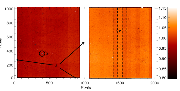
Figure 10: Normalized IRDIS master-flat image in $H$ band. The illuminated detector halves are surrounded by the field-mask {a}. The masked regions (and all pixels with value $<0.1$) are set to $1000$ and shown as white in this image. This enhances several clusters of dead and hot pixels (e.g., {b} around [x,y] $\approx$ [400,400]). A time varying read-out signature of the detector is visible as columns of 64 pixels wide (e.g., {c}).

Raw IRDIS frames consist of $2048$ by $1024$ pixels in the $x$ & $y$ directions, respectively. The two beams separated by the beam splitter (see Sect. 3.2) are centered roughly on the left and right detector halves, while a field mask avoids leakage of signal from one half to the other.

We median combine all dark + background observations taken with DIT = 16 s to create a master-dark image. From internal light source (flat-field) measurements, we create a (dark-subtracted) master-flat image: we take median over two regions of $800\,{\times}\,800$ centered on the left half ([$x,y$] = [512, 512]) and the right half ([$x,y$] = [1536,512]) and use this value to normalize. To avoid emphasizing dead pixels or pixels masked by the field mask, we change all pixel values $<0.1$ into $1000$. The final master-flat is shown in Fig. 10. Note that the master-flat still contains a vertical read-out pattern (features c in Fig. 10). It is difficult to distinguish between the flat signal and this pattern, and polarimetry requires that we maintain the different transmission ratios of the two detector halves in our master-flat (hence the single normalization earlier). Therefore, we have chosen to leave the master-flat uncorrected for this pattern and remove these read-out columns at a later stage in the post-processing (Sect.4.1).

Preferably, to correct for background signal we would have used ’SKY’ observations: observations taken with the same DIT as the science (or ’OBJECT’) frames, recorded on-sky with the star moved out of the detector FOV. Such SKY images contain background emission from possible interstellar origin (e.g., from nearby nebulosity), the earth atmosphere, the optical system and the detector dark current. Because there were no SKY images recorded for these observations, we corrected for instrument background emission by subtracting the master-dark from each science frame recorded of TW Hydrae. Subsequently, we divide the science frames by the master-flat to correct for flat-field errors. Next, we crop the frames to separate the left ($1\leq x\leq 1024$) from the right ($1025\leq x\leq 2048$) detector half.

To align the central star with the center of the image one could use the ’CENTER’ frames, where SPHERE’s DM has created satelite spots around the star-center. However, because alignment between individual frames is a crucial element of PDI we opted for an alternative multi-stage approach. We find the centers of the star in both left and right frame by cross-correlation with a two-dimensional Moffat function, where the central pixels within a radius of six pixels are set to zero to account for the coronagraph mask. We determine $I$ according to Eq. 5, and median combine the images of all HWP cycles to create a template image. To enhance our frame-to-frame alignment, we repeat the cross-correlation for all frames, this time using the template image. Due to irregular diffraction paterns close to the edge of the coronagraph mask, we cannot guarantee with the two centering steps described above that the star-center lies at the center of the image. However, it does place the star close to the center of the image, and accurately alligns all frames with respect to each other. The latter is crucial to perform the single and double-difference subtractions. A more advanced centering is performed at a later stage.